Submitted:
31 January 2024
Posted:
02 February 2024
You are already at the latest version
Preprints on COVID-19 and SARS-CoV-2
Abstract
This study rigorously investigates the impact of COVID-19 on the Tunisian stock market volatility. The investigation spans from January 2020 to December 2022, employing a GJR-GARCH model, bias-corrected wavelet analysis, and an ARDL approach. Specific variables related to health measures and government interventions are incorporated. The findings highlight that confirmed and death cases contribute significantly to the escalation in TUNINDEX volatility. Interestingly, certain indices related to government interventions exhibit no substantial impact on volatility, indicating a weak resilience of the Tunisian stock market amidst the challenges posed by COVID-19. However, the application of the bias-corrected wavelet analysis yields more nuanced outcomes in terms of correlations of volatility to the same metrics. Notably, the study recognizes the potential influence of uncertainties linked to the duration of lockdowns on financial market volatility. The positive and long-term impact on volatility of the US Equity Market uncertainty and VIX is evident through the Autoregressive Distributed Lag Model (ARDL), whereas economic policy uncertainty shows no significant impact. This indicates a potential vulnerability of the Tunisian stock market to future shocks, emphasizing the need for government efforts to instill investor confidence. This comprehensive exploration contributes to our understanding of the dynamics between the pandemic’ metrics, government interventions, and financial market stability. Our findings provide valuable insights for implementing risk management strategies amid the COVID‐19 crisis.
Keywords:
Stock return volatility
; COVID-19
; Uncertainty
; GARCH
; Bias-corrected Wavelet coherence analysis
; ARDL
1. Introduction
The outbreak of the COVID-19 pandemic has triggered unprecedented challenges across global financial markets, with profound implications for economic systems and investment landscapes (see Lee et al., 2020; He et al., 2020; Ashraf, 2020; Okori and Lin, 2021; Mazur et al., 2021; Endri et al., 2021; Chowdhury et al., 2022). Among the affected regions, Tunisia has encountered distinctive dynamics in its stock market, marked by heightened volatility and fluctuations. This research endeavors to comprehensively examine the Impact of COVID-19 on the Tunisian stock market volatility through the lens of a GJR-GARCH model, Wavelet Coherence Analysis, and Autoregressive Distributed Lag Model (ARDL). The motivation behind this study stems from the critical need to understand and quantify the specificities of the financial repercussions experienced by Tunisia in the wake of the pandemic, shedding light on the relationships between key variables influencing market dynamics. The significance of this research lies in its potential to provide valuable insights for investors, policymakers, and financial analysts navigating during and the post-COVID economic recovery, facilitating informed decision-making in the Tunisian financial landscape.
Our research is distinguished by incorporating specific determinants related to the COVID-19 pandemic and aims to quantify their impact on the conditional volatility of TUNINDEX stock market return. It is also important to investigate the predictive power of uncertainty indicators for volatility in the Tunisian context while considering a very sensitive period of investigation. By doing so, we not only offer a thorough exploration of a burgeoning economy grappling with the pandemic but also contribute valuable insights, particularly in light of the scarce existing literature within the scope of our research goals.
The remainder of this paper is as follows. Section 2 reviews specific studies that relate the stock market volatility to the COVID-19 crisis. Section 3 presents data and materials to answer the research objective. The main findings are exposed in Section 4. Concluding remarks and policy implications of the results are displayed in Section 5 and Section 6, respectively.
2. Literature review
Literature on the determinants of stock market volatility is abundant (see Binder and Merges, 2001; Mazzucato and Semmler, 2002; Nikmanesh and Nor, 2016; Hussain et al., 2019; Hewamana et al., 2022; Biu and Kusuma, 2023; Dhingra et al., 2023; etc.). We particularly focus on research that relates stock market volatility to the COVID-19 crisis. Li et al. (2022) established a link between COVID-19 fear and stock market volatility, emphasizing its significance for portfolio diversification. Findings suggest that COVID-19 fear is a primary driver of public attention and stock market fluctuations, with associated impacts on both stock returns and GDP during the pandemic. Gao et al. (2022) used the quantile-on-quantile approach to compare the impact of COVID-19 new cases on U.S. and Chinese stock market volatility, revealing COVID-19 as the primary driver in the U.S. with implications for monetary policy and market stability amid the global spread of the virus. Kusumahadi and Permanan (2021) examined the global impact of COVID-19 on stock return volatility in 15 countries and identified structural changes preceding the onset of COVID-19, suggesting the positive influence of the virus on return volatility, though the effect size is modest. Uddin et al. (2021) emphasized the importance of leveraging economic factors such as capitalism, monetary policy, and financial development in policymaking to address global stock market volatility and prevent potential financial crises. Bora and Basistha (2021) compared the stock return volatility performance of India pre and during the COVID-19 crisis and documented a higher volatility due to the pandemic effect. According to Baek et al. (2020), COVID-19 news significantly influences US stock market volatility, with a notable negativity bias, and industry-wise changes in systematic risk. Yousef (2020) used regression analysis and GARCH models to show that the COVID-19 pandemic, daily new cases, and growth rate of daily new cases significantly increased volatility across all G7 stock indices. The same view is shared by Izzeldin et al. (2021). Through GARCH modeling, Chaudhary et al. (2020) found a negative mean return during the COVID period, with heightened volatility, suggesting a bearish trend in the top 10 countries according to GDP. The global COVID-19 fear index seems to have a pronounced effect on the volatility of 19 emerging stock markets (see Sadiq et al., 2021). Papadamou et al. (2020) highlighted that increased anxiety regarding COVID-19 contagion on Google correlates with heightened risk aversion in stock markets, especially in Europe. The volatility in stock prices caused by COVID-19 affects abnormal returns, prompting investors to implement risk management strategies amid uncertainty, while also creating potential speculative opportunities in an inefficient market (En-dri et al., 2021). Lúcio and Caiado (2022) observed that amid the COVID-19 outbreak, all S&P 500 industries, except Internet and Direct Marketing Retail, witnessed a substantial rise in volatility, leading to a convergence in time-varying variance among them.
Studies on the effect of COVID-19 on stock return volatility in the Tunisian context are very recent. Using GARCH models, Akinlaso et al. (2022) detected high persistence in both Tunisia’s Islamic and conventional stock markets, with the conventional index negatively influencing Islamic stocks during the pandemic. Jeribi et al. (2015) and Fakhfekh et al. (2023) revealed increased volatility persistence in all Tunisian sectorial stock market indices post-COVID-19, with certain sectors showing significant asymmetric effects.
3. Data and Methodology
3.1. Data
We collect daily data on TUNINDEX returns amid the COVID-19 pandemic. The period spans from January 2d, 2020 to December, 30th 2022, making a total of 755 observations, omitting nontrading days. Since the objective is to analyze the impact of the sanitary crisis on the Tunisian stock return volatility, we gather data on the number of cases (total, new, and death) and on the government intervention to limit the spread of the virus (see Table 1 for details).

Table 1.
Data definitions.
| Variable | Symbol | Definition | Source |
| TUNINDEX | tun | The daily closing price of the Tunisian market index | https://www.investing.com/indices/tunindex-historical-data |
| Total cases | total_cases | Cumulative number of the confirmed cases due to COVID-19 | Our World in Data https://ourworldindata.org/coronavirus/country/tunisia |
| Total deaths | total_death | Cumulative number of the confirmed death cases due to COVID-19 | |
| New cases | new_cases | Total number of the new confirmed cases due to COVID-19 | |
| New deaths | new_death | Total number of new confirmed death cases due to COVID-19 | |
| Rate of confirmed cases | cases_rate | News cases/Total cases | Calculus |
| Rate of deaths | death_rate | Death cases/Total deaths | Calculus |
| Stringency index | stringency_index | Ranges from 0 to 100, where higher values indicate stricter government policies and restrictions in response to the COVID-19 pandemic. |
Oxford COVID-19 Government Response Tracker (OxCGRT) https://github.com/OxCGRT/covid-policy-dataset |
| Containment health index | containement_health_index | Typically ranges from 0 to 100, where higher values indicate better virus containment. |
|
| Economic policy index | economic_policy_index | Ranges from 0 to 100, where higher values indicate a more accommodative economic policy stance and lower values indicate a more restrictive stance. |
|
| Government response index | government_response_index | Ranges between 0 and 100. A higher score means a better country’s response to the pandemic. | |
| WTI crude oil price | wti_price | Crude oil price (United States) | Energy Information Administration database https://www.eia.gov/dnav/pet/pet_pri_spt_s1_d.htm |
| School closing | s1 | Sub-indicator 1 of the stringency index | Oxford COVID-19 Government Response Tracker (OxCGRT) https://github.com/OxCGRT/covid-policy-dataset |
| Workplace closing | s2 | Sub-indicator 2 of the stringency index | |
| Cancel public events | s3 | Sub-indicator 3 of the stringency index | |
| Restrictions on public gatherings | s4 | Subindicator 4 of the stringency index | |
| Closures of public transport | s5 | Sub-indicator 5 of the stringency index | |
| Stay-at-home requirements | s6 | Sub-indicator 6 of the stringency index | |
| Restrictions on internal movements | s7 | Subindicator 7 of the stringency index | |
| International travel control | s8 | Sub-indicator 8 of the stringency index | |
| Public information gatherings | s9 | Subindicator 9 of the stringency index |
Source: The Author.
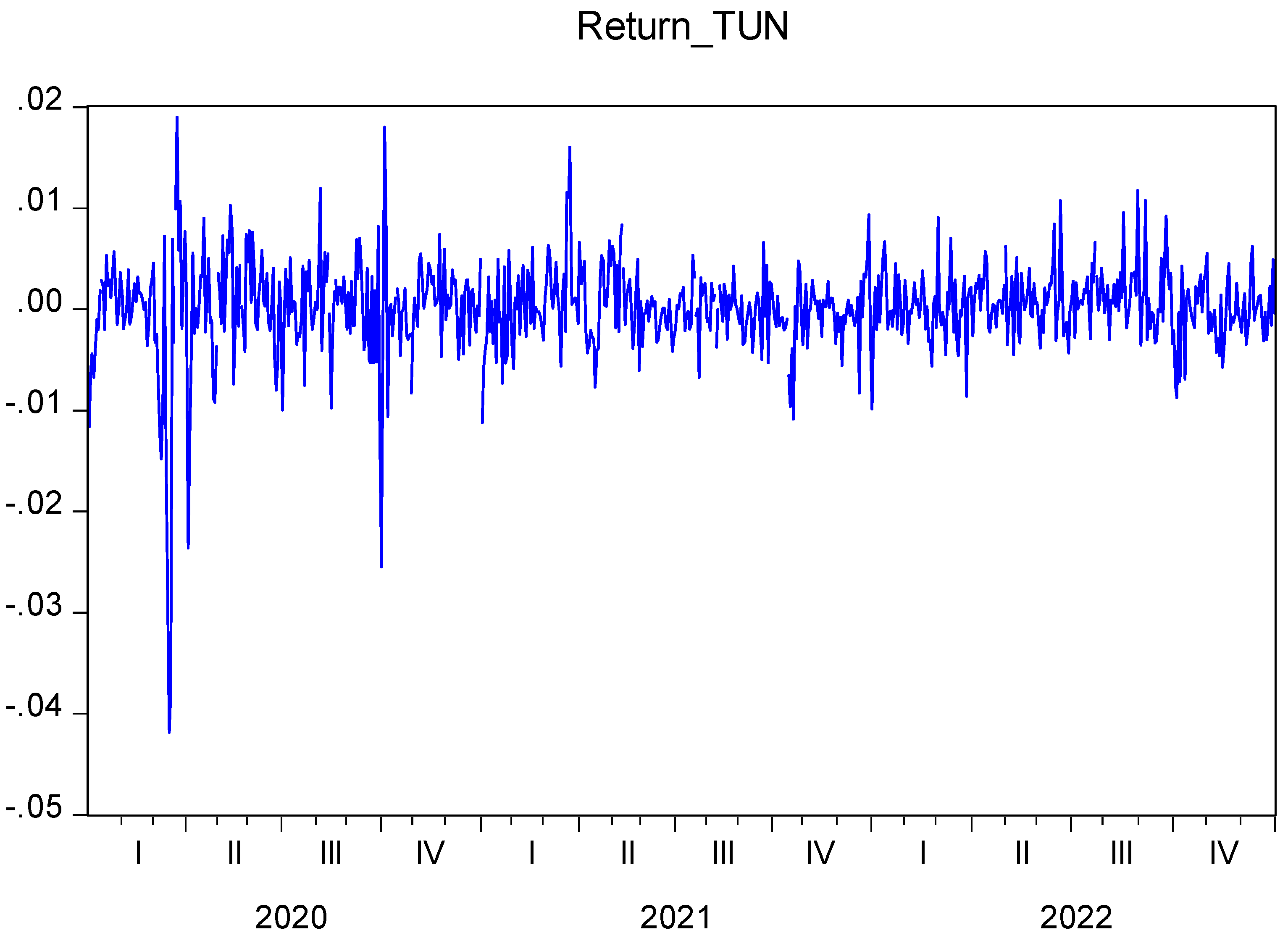
Descriptive statistics of the above variables are displayed in Table 2. The TUNINDEX exhibits a mean return of 0.000150, indicating a generally modest performance. Figure 1 illustrates a compelling narrative of diminishing returns in TUNINDEX, particularly during the challenging times of the COVID-19 era. The total number of COVID-19 cases and deaths, with means of 551,839.1 and 16,432.85 respectively, reflects the significant impact of the pandemic on public health. The stringency index, with a mean of 49.03363, suggests varying degrees of government measures. Interestingly, the containment health index, economic support index, and government response index do not seem to strongly influence market volatility. The skewness values, particularly for TUNINDEX, indicate a negatively skewed distribution, and the kurtosis values suggest heavy tails in the distribution.
Table 2.
Descriptive statistics of the variables.
| RETURN_TUN | TOTAL_CASES | TOTAL_DEATHS | STRINGENCY_INDEX | S1 | S2 | S3 | S4 | S5 | S6 | S7 | S8 | S9 | CONTAINMENT_HEALTH_INDEX | ECONOMIC_SUPPORT_INDEX | GOVERNMENT_RESPONSE_INDEX | WTI_OIL_RETURN | |
| Mean | 0.000150 | 551839.1 | 16432.85 | 49.03363 | 1.034043 | 1.144681 | 1.597163 | 3.262411 | 0.307801 | 0.808511 | 0.639716 | 1.876596 | 1.846809 | 50.28391 | 46.84397 | 49.85403 | 0.001816 |
| Median | 0.000339 | 603981.0 | 21941.00 | 45.31000 | 1.000000 | 1.000000 | 2.000000 | 4.000000 | 0.000000 | 0.000000 | 0.000000 | 2.000000 | 2.000000 | 49.96000 | 50.00000 | 48.80000 | 0.002294 |
| Maximum | 0.018974 | 1147571. | 29284.00 | 90.74000 | 3.000000 | 3.000000 | 2.000000 | 4.000000 | 2.000000 | 2.000000 | 2.000000 | 4.000000 | 2.000000 | 77.74000 | 75.00000 | 77.40000 | 0.425832 |
| Minimum | -0.041859 | 1.000000 | 3.000000 | 0.000000 | 0.000000 | 0.000000 | 0.000000 | 0.000000 | 0.000000 | 0.000000 | 0.000000 | 0.000000 | 0.000000 | 0.000000 | 0.000000 | 0.000000 | -0.281382 |
| Std. Dev. | 0.004802 | 444625.6 | 11959.82 | 21.88917 | 1.017728 | 0.804146 | 0.757157 | 1.546832 | 0.603267 | 0.967621 | 0.918936 | 1.122006 | 0.490616 | 18.04488 | 25.69635 | 17.32935 | 0.045112 |
| Skewness | -2.203420 | 0.060338 | -0.263656 | -0.119352 | 0.546806 | 0.438110 | -1.480724 | -1.632203 | 1.799000 | 0.390066 | 0.772150 | 0.298314 | -3.148689 | -1.074264 | -0.287851 | -1.055407 | 1.353766 |
| Kurtosis | 20.12168 | 1.393214 | 1.331061 | 2.671155 | 2.097217 | 2.843062 | 3.384040 | 3.672980 | 4.993379 | 1.183648 | 1.632938 | 2.231494 | 11.52594 | 4.109855 | 1.785051 | 4.541901 | 29.12992 |
| Jarque-Bera | 9181.807 | 72.04800 | 83.47809 | 4.850368 | 59.07326 | 23.27648 | 261.9562 | 326.3342 | 497.0006 | 114.7899 | 124.9530 | 27.80539 | 3300.243 | 171.7835 | 53.09627 | 200.7193 | 20271.78 |
| Probability | 0.000000 | 0.000000 | 0.000000 | 0.088462 | 0.000000 | 0.000009 | 0.000000 | 0.000000 | 0.000000 | 0.000000 | 0.000000 | 0.000001 | 0.000000 | 0.000000 | 0.000000 | 0.000000 | 0.000000 |
| Sum | 0.105709 | 3.68E+08 | 10747083 | 34568.71 | 729.0000 | 807.0000 | 1126.000 | 2300.000 | 217.0000 | 570.0000 | 451.0000 | 1323.000 | 1302.000 | 35450.16 | 33025.00 | 35147.09 | 1.280245 |
| Sum Sq. Dev. | 0.016235 | 1.31E+14 | 9.34E+10 | 337311.6 | 729.1830 | 455.2426 | 403.5943 | 1684.454 | 256.2071 | 659.1489 | 594.4879 | 886.2638 | 169.4553 | 229234.8 | 464852.8 | 211415.7 | 1.432724 |
| Observations | 705 | 666 | 654 | 705 | 705 | 705 | 705 | 705 | 705 | 705 | 705 | 705 | 705 | 705 | 705 | 705 | 705 |
Source: The Author.
Figure 1.
Evolution of TUNINDEX stock return (02/01/2020-30/12/2022). Source: The Author.
3.2. Methodology
The assessment of volatility has mandated the application of models within the Autoregressive Conditional Heteroskedasticity (ARCH) framework in the realm of financial literature. Originating with the seminal ARCH model introduced by Engle (1982), subsequent advancements have been made, encompassing the development of models such as Generalized ARCH (GARCH), GARCH-in-mean, Quadratic GARCH, and Threshold GARCH, among others.
The stock return is calculated following previous related literature using this formula:
where are the stock market indices of the Tunisian Stock Exchange at times t and t-1, respectively. Ln is the natural logarithm.
The logarithm transformation serves as a technique to induce stationarity in variables by mitigating trends and seasonality within time series data. Consequently, Augmented Dickey-Fuller (ADF) and Phillips-Perron (PP) tests are conducted to verify the attainment of stationarity in the level of returns. The associated results are available in Table 3.
The autoregressive (AR) (p) or autoregressive moving average (ARMA) (p, q) structures are commonly integrated as explanatory elements within the conditional mean equation of Generalized Autoregressive Conditional Heteroskedasticity (GARCH) models for the dependent variable. Following Insaidoo et al. (2021), an advantageous feature of the GARCH model lies in its adaptability to include explanatory variables and dummy variables in both the conditional mean and variance equations, thereby accommodating the specific objectives of the study. Hence, we incorporate each of the COVID-19 variables and the government intervention controls in both the mean equation and the variance equation, separately to capture the effect of the pandemic on the Tunisian stock return and volatility. Our econometric modeling is essentially based on Fakhfekh et al. (2023). However, we distinguish from their study by including specific controls related to the sanitary crisis instead of separating pre-crisis and during-crisis periods. Thus, we estimate the following GARCH family models.
Table 3.
Results of ARCH/GARCH family models for the TUNINDEX volatility and oil volatility.
| Panel A: Stock return volatility | ||||||||
| Model | ARCH(1), constant | ARCH(1), AR(1) | ARCH(1), MA(1) | ARCH(1), ARMA(1,1) | GARCH(1,1), constant | GARCH(1,1), AR(1) | GARCH(1,1), MA(1) | GARCH(1,1), ARMA(1,1) |
| AIC | -8.248105 | -8.283928 | -8.274759 |
-8.281654 |
-8.332585 |
-8.376225 |
-8.365392 |
-8.378094 |
| SC | -8.229721 |
-8.259390 |
-8.250246 |
-8.250982 |
-8.308073 |
-8.345553 |
-8.334751 |
-8.341287 |
| Model | EGARCH(1,1), constant | EGARCH(1,1), AR(1) | EGARCH(1,1), MA(1) | EGARCH(1,1), ARMA(1,1) | TGARCH(1,1), constant | TGARCH(1,1), AR(1) | TGARCH(1,1), MA(1) | TGARCH(1,1), ARMA(1,1) |
| AIC | -8.323690 |
-8.369747 |
-8.358517 |
-8.369772 |
-8.330636 |
-8.374358 |
-8.363444 |
-8.376183 |
| SC | -8.293050 |
-8.332940 |
-8.321748 |
-8.326830 |
-8.299996 |
-8.337551 |
-8.326675 |
-8.333242 |
| Panel B: WTI oil volatility | ||||||||
| Model | ARCH(1), constant | ARCH(1), AR(1) | ARCH(1), MA(1) | ARCH(1), ARMA(1,1) | GARCH(1,1), constant | GARCH(1,1), AR(1) | GARCH(1,1), MA(1) | GARCH(1,1), ARMA(1,1) |
| AIC | -3.856832 |
-3.990224 |
-4.003052 |
-4.000366 |
-4.272393 |
-4.269562 |
-4.269562 |
-4.257070 |
| SC | -3.837436 |
-3.964362 |
-3.977190 |
-3.968039 |
-4.246531 |
-4.237234 |
-4.237235 |
-4.231253 |
| EGARCH(1,1), constant | EGARCH(1,1), AR(1) | EGARCH(1,1), MA(1) | EGARCH(1,1), ARMA(1,1) | TGARCH(1,1), constant | TGARCH(1,1), AR(1) | TGARCH(1,1), MA(1) | TGARCH(1,1), ARMA(1,1) | |
| AIC | -4.278102 |
-4.275790 |
-4.275864 |
-3.344925 |
-4.292975 |
-4.290166 |
-4.290171 |
-4.287428 |
| SC | -4.245774 |
-4.236997 |
-4.237071 |
-3.299666 |
-4.260648 |
-4.251373 |
-4.251377 |
-4.242170 |
Source: The Author.
3.2.1. ARCH
The ARCH model characterizes the variance of a time series, particularly in situations involving dynamic and potentially volatile variance. It was introduced by Engle (1982). While ARCH models can potentially depict a slowly escalating variance trend over time, their primary application lies in scenarios featuring brief episodes of heightened variation. It is worth noting that situations involving a gradual increase in both variance and mean level may be more effectively addressed by transforming the variable.
The mean equation is written as follows:
The choice between AR(1), MA(1), and ARMA(1,1) is made based on the conventional information criteria (Aikake, Schwarz) for which
the value is minimized.
Our estimations show that AR(1) is the preferred one.
The conditional variance equation is defined as:
where . This model is known as the linear ARCH(p). In
financial data analysis, the model captures the phenomenon of volatility
clustering, wherein significant (insignificant) price changes tend to be
succeeded by other substantial (moderate) price changes, but with an
unpredictable direction. To streamline the model and guarantee a consistently
diminishing impact of more distant shocks, a makeshift linearly declining lag
structure was frequently enforced in many early applications of the model (see Bollerslev et al., 1992; Bollerslev and Mikkelsen, 1996).
3.2.2. GARCH
Bollerslev’s GARCH model (1986) is the most widely used model for estimating volatility. volatility. GARCH models have had great success in the literature due to their simple specification and ease of interpretation.
The conditional variance equation is defined as:
where . For a GARCH(1,1), the constraint < 1 implies that the unconditional variance of the ε yield series is finite and that the conditional variance evolves. It also provides the necessary and sufficient for the stochastic process ; t ∈ Z to be a unique process strictly stationary with E() < ∞.
Two key properties can be noted from the above equation. First, a high value of or gives rise to a high value of and this generates the volatility clustering that is common in time series. Second, the tail distribution is thicker than that of a normal distribution (see Mestiri, 2022).
3.2.4. EGARCH
This model is suggested by Nelson (1991) to account for leverage effects. It is an asymmetric Exponential GARCH specification that distinguishes between “good” and “bad” news on volatility.
The conditional volatility equation is given by:
If there is "good" news, and the total effect is given by . If there is "bad" news, , and the total effect is given by . “Bad” news is likely to have a more pronounced impact on volatility and is expected to be negative.
3.2.5. GJR-GARCH
Another version of an asymmetric GARCH model with leverage effects is the Threshold GARCH specification, called also GJR-GARCH. The conditional volatility is given by:
With
When , the total effect is given by . If , the total effect is given by . The coefficient is expected to be positive so that “bad” news has a larger impact on volatility.
The best-fit model is chosen based on Akaike (AIC) and Schwarz (SC) information criteria for which the value is minimized.
According to Bera and Higgins (1993), the most applied financial work shows that GARCH (1,1) provides a flexible and parsimonious approximation of the conditional variance dynamics and is capable of representing the majority of financial series. Therefore, p=1 and q=1 are applied for all GARCH family models to be estimated.
Before estimating ARCH-type models, we need to test for the presence of ARCH(q) effects. We rely on the Lagrange Multiplier (LM) test. We reject the null hypothesis of no ARCH effects (F-statistic=342.0031, p-value=0.000; Obs*R2=235.6154, p-value=0.000).
To know what a combination of variables is to be included in the regression we provide the pairwise correlation matrix (see supplemental file for details).
4. Results and discussion
4.1. Impact of COVID-19 announcements and government intervention on TUNINDEX stock return volatility
Table 3 shows that GJR-GARCH is the preferred one as the conventional information criteria exhibit the lowest values. To examine the impact of COVID-19 announcements and the government intervention variables, we regress the conditional stock return variance that results from the GJR-GARCH(1,1), AR(1) model on the variables of interest and a set of controls (see Ibrahim et al., 2020; Bakry et al., 2022):
where CR: cases_rate, DR: death_rate, GRI: Government intervention index (this includes stringency_index, containment_health_index, economic_support_index, government_response_index, and subindicators of the stringency index (s1 to s9), Oil_Vol: Conditional WTI oil volatility from GJR-GARCH(1,1) with a constant.
To handle the multicollinearity issue, we include the government intervention indicators separately. Further, we control for autocorrelation and heteroscedasticity by estimating the equation with the Newey-West method. Results are available in Table 4 and Table 5. We re-estimate the variants of the equations while skipping for the cases_rate variable. All results duplicate mostly the ones in Table 4 and Table 5, except that death_rate becomes statistically significant (see Table 6 and Table 7).
According to Kamal and Wohar (2023), "Considering global market integration (Solnik, 1974) and to remove misspecification error, [..]. We also lagged the independent variables by one period to examine the slow response of the market. Slow response supports the underreaction hypothesis, which suggests investors adjust slowly to new information.". We replicate the output while considering the variables of interest and controls lagged with one period (see Table 8, Table 9, Table 10 and Table 11).
The observed incidence of confirmed cases and mortality rates exhibit a positive association with heightened volatility in the TUNINDEX in addition to the WTI conditional volatility. Moreover, there exists a positive correlation between the stringency index and volatility in the Tunisian stock market. Conversely, the indices about containment health economic support and government response do not manifest a discernible impact on market volatility. Those observations can be attributed to increased uncertainty and economic impacts. Rising cases make investors cautious, leading to market fluctuations. Stringent government measures, reflected in the stringency index, also correlate positively with market volatility, indicating economic repercussions. However, indices related to health economic support and government response show no significant impact on volatility, suggesting that other factors may be more influential in shaping the Tunisian stock market.
Table 4.
Effect of COVID-19 announcements and government intervention on TUNINDEX volatility.
| Eq Name: | EQ01 | EQ02 | EQ03 | EQ04 |
| C | 0.000011 | 0.000011 | 0.000011 | 0.000011 |
| [10.9061]*** | [11.0044]*** | [11.6222]*** | [11.3206]*** | |
| CASES_RATE | 0.000359 | 0.000358 | 0.000389 | 0.000366 |
| [3.3678]*** | [3.3480]*** | [3.2211]*** | [3.2644]*** | |
| DEATH_RATE | 0.000049 | 0.000053 | 0.000010 | 0.000037 |
| [0.7213] | [0.7701] | [0.1111] | [0.4705] | |
| CONDVAR_WTI | 0.001224 | 0.001220 | 0.001185 | 0.001219 |
| [2.3954]** | [2.3831]** | [2.3961]** | [2.3998]** | |
| DSTRINGENCYINDEX | 0.000001 | |||
| [0.9286] | ||||
| DCONTAINMENTHEALTHINDEX | 0.000001 | |||
| [0.7738] | ||||
| DECONOMICSUPPORTINDEX | 0.000001 | |||
| [1.2960] | ||||
| DGOVERNMENTRESPONSEINDEX | 0.000001 | |||
| [0.9220] | ||||
| Observations: | 654 | 654 | 654 | 654 |
| R-squared: | 0.4811 | 0.4794 | 0.4907 | 0.4823 |
| F-statistic: | 150.4010 | 149.4343 | 156.3274 | 151.1775 |
| Prob(F-stat): | 0.0000 | 0.0000 | 0.0000 | 0.0000 |
Note: *, **, *** significant at 10%, 5% and 1%, respectively. Source: The Author.
Table 5.
Effect of stringency index sub-indicators on TUNINDEX volatility.
| Eq Name: | EQ01 | EQ02 | EQ03 | EQ04 | EQ05 | EQ06 | EQ07 | EQ08 | EQ09 |
| C | 0.000011 | 0.000011 | 0.000011 | 0.000011 | 0.000011 | 0.000011 | 0.000011 | 0.000011 | 0.000011 |
| [10.4573]*** | [10.8456]*** | [10.3587]*** | [17.3295]*** | [10.6964]*** | [11.0051]*** | [10.7373]*** | [10.4448]*** | [10.4588]*** | |
| CASES_RATE | 0.000348 | 0.000355 | 0.000346 | 0.000367 | 0.000353 | 0.000368 | 0.000345 | 0.000348 | 0.000348 |
| [3.4899]*** | [3.4638]*** | [3.5209]*** | [10.9008]** | [3.4494]*** | [3.3898]*** | [3.3523]*** | [3.5048]*** | [3.4969]*** | |
| DEATH_RATE | 0.000077 | 0.000058 | 0.000075 | 0.000024 | 0.000068 | 0.000041 | 0.000082 | 0.000076 | 0.000076 |
| [1.3980] | [0.9628] | [1.3625] | [0.9679] | [1.1819] | [0.6740] | [1.3229] | [1.3816] | [1.3822] | |
| CONDVAR_WTI | 0.001212 | 0.001233 | 0.001221 | 0.001232 | 0.001209 | 0.001203 | 0.001213 | 0.001213 | 0.001213 |
| [2.3589]** | [2.4250]** | [2.3817]** | [8.2596]*** | [2.3672]** | [2.3704]** | [2.3559]** | [2.3603]** | [2.3588]** | |
| D(S1) | -0.000002 | ||||||||
| [-0.7363] | |||||||||
| D(S2) | 0.000008 | ||||||||
| [1.0688] | |||||||||
| D(S3) | 0.000005 | ||||||||
| [0.6859] | |||||||||
| D(S4) | 0.000011 | ||||||||
| [4.5894]*** | |||||||||
| D(S5) | 0.000007 | ||||||||
| [0.8645] | |||||||||
| D(S6) | 0.000016 | ||||||||
| [1.6222] | |||||||||
| D(S7) | -0.000002 | ||||||||
| [-0.3753] | |||||||||
| D(S8) | -0.000002 | ||||||||
| [-0.7549] | |||||||||
| D(S9) | 0.000004 | ||||||||
| [4.7152]*** | |||||||||
| Observations: | 654 | 654 | 654 | 654 | 654 | 654 | 654 | 654 | 654 |
| R-squared: | 0.4766 | 0.4808 | 0.4773 | 0.4928 | 0.4777 | 0.4938 | 0.4767 | 0.4764 | 0.4764 |
| F-statistic: | 147.7157 | 150.2575 | 148.1492 | 157.6232 | 148.3977 | 158.2759 | 147.8009 | 147.6410 | 147.6070 |
| Prob(F-stat): | 0.0000 | 0.0000 | 0.0000 | 0.0000 | 0.0000 | 0.0000 | 0.0000 | 0.0000 | 0.0000 |
Note: *, **, *** significant at 10%, 5% and 1%, respectively. Source: The Author.
Table 6.
Effect of COVID-19 announcements and government intervention on TUNINDEX volatility, excluding cases_rate.
Table 6.
Effect of COVID-19 announcements and government intervention on TUNINDEX volatility, excluding cases_rate.
| Eq Name: | EQ01 | EQ02 | EQ03 | EQ04 | EQ05 |
| C | 0.000012 | 0.000012 | 0.000012 | 0.000012 | 0.000012 |
| [10.9188]*** | [10.7714]*** | [11.0068]*** | [11.7608]*** | [11.1964]*** | |
| DEATH_RATE | 0.000226 | 0.000217 | 0.000221 | 0.000212 | 0.000218 |
| [4.7771]*** | [4.4689]*** | [4.3267]*** | [3.4279]*** | [3.9955]*** | |
| CONDVAR_WTI | 0.001680 | 0.001692 | 0.001686 | 0.001689 | 0.001689 |
| [2.0681]** | [2.0647]** | [2.0570]** | [2.0576]** | [2.0545]** | |
| DSTRINGENCYINDEX | 0.000000 | ||||
| [0.6286] | |||||
| DCONTAINMENTHEALTHINDEX | 0.000000 | ||||
| [0.3755] | |||||
| DECONOMICSUPPORTINDEX | 0.000000 | ||||
| [0.8845] | |||||
| DGOVERNMENTRESPONSEINDEX | 0.000000 | ||||
| [0.5446] | |||||
| Observations: | 654 | 654 | 654 | 654 | 654 |
| R-squared: | 0.3916 | 0.3923 | 0.3916 | 0.3928 | 0.3919 |
| F-statistic: | 139.4355 | 139.8593 | 139.4782 | 140.1365 | 139.6133 |
| Prob(F-stat): | 0.0000 | 0.0000 | 0.0000 | 0.0000 | 0.0000 |
: *, **, *** significant at 10%, 5% and 1%, respectively. Source: The Author.
Table 7.
Effect of stringency index sub-indicators on conditional stock return volatility, excluding cases_rate.
Table 7.
Effect of stringency index sub-indicators on conditional stock return volatility, excluding cases_rate.
| Eq Name: | EQ01 | EQ02 | EQ03 | EQ04 | EQ05 | EQ06 | EQ07 | EQ08 | EQ09 |
| C | 0.000012 | 0.000012 | 0.000012 | 0.000012 | 0.000012 | 0.000012 | 0.000012 | 0.000012 | 0.000012 |
| [10.9181]*** | [11.0699]*** | [10.8839]*** | [11.1801]*** | [11.0729]*** | [10.9574]*** | [11.1625]*** | [10.9210]*** | [10.9188]*** | |
| DEATH_RATE | 0.000227 | 0.000216 | 0.000223 | 0.000195 | 0.000225 | 0.000207 | 0.000238 | 0.000226 | 0.000226 |
| [4.8043]*** | [4.3602]*** | [5.0099]*** | [3.8221]*** | [4.5418]*** | [4.3190]*** | [4.6804]*** | [4.7765]*** | [4.7771]*** | |
| CONDVAR_WTI | 0.001679 | 0.001700 | 0.001689 | 0.001712 | 0.001681 | 0.001693 | 0.001668 | 0.001681 | 0.001680 |
| [2.0665]** | [2.0838]** | [2.0807]** | [2.0813]** | [2.0665]** | [2.0689]** | [2.0528]** | [2.0688]** | [2.0681]** | |
| D(S1) | -0.000002 | ||||||||
| [-0.8260] | |||||||||
| D(S2) | 0.000005 | ||||||||
| [1.0467] | |||||||||
| D(S3) | 0.000008 | ||||||||
| [0.8771] | |||||||||
| D(S4) | 0.000008 | ||||||||
| [1.5721] | |||||||||
| D(S5) | 0.000001 | ||||||||
| [0.3585] | |||||||||
| D(S6) | 0.000012 | ||||||||
| [1.5046] | |||||||||
| D(S7) | -0.000006 | ||||||||
| [-1.6216] | |||||||||
| D(S8) | -0.000001 | ||||||||
| [-0.3842] | |||||||||
| D(S9) | 0.000006 | ||||||||
| [6.3409]*** | |||||||||
| Observations: | 654 | 654 | 654 | 654 | 654 | 654 | 654 | 654 | 654 |
| R-squared: | 0.3920 | 0.3933 | 0.3939 | 0.3999 | 0.3915 | 0.4004 | 0.3948 | 0.3915 | 0.3916 |
| F-statistic: | 139.6728 | 140.4515 | 140.8341 | 144.3825 | 139.3918 | 144.7011 | 141.3569 | 139.3879 | 139.4355 |
| Prob(F-stat): | 0.0000 | 0.0000 | 0.0000 | 0.0000 | 0.0000 | 0.0000 | 0.0000 | 0.0000 | 0.0000 |
Note: *, **, *** significant at 10%, 5% and 1%, respectively. Source: The Author.
Table 8.
Effect of lagged COVID-19 announcements and government intervention on conditional stock return volatility.
Table 8.
Effect of lagged COVID-19 announcements and government intervention on conditional stock return volatility.
| Eq Name: | EQ01 | EQ02 | EQ03 | EQ04 | EQ05 |
| C | 0.000011 | 0.000011 | 0.000011 | 0.000011 | 0.000011 |
| [12.7748]*** | [12.5856]*** | [12.7677]*** | [13.5131]*** | [12.9403]*** | |
| CASES_RATE(-1) | 0.000286 | 0.000298 | 0.000296 | 0.000300 | 0.000301 |
| [2.9352]*** | [2.8389]** | [2.8335]*** | [2.8340]*** | [2.7877]*** | |
| DEATH_RATE(-1) | 0.000093 | 0.000064 | 0.000070 | 0.000069 | 0.000061 |
| [1.8091] | [0.9606] | [1.0295] | [0.7853] | [0.7971] | |
| CONDVAR_WTI(-1) | 0.001005 | 0.001017 | 0.001013 | 0.000996 | 0.001011 |
| [2.2048]** | [2.2664]** | [2.2434]** | [2.2277]** | [2.2419]** | |
| DSTRINGENCYINDEX(-1) | 0.000001 | ||||
| [0.9800] | |||||
| DCONTAINMENTHEALTHINDEX(-1) | 0.000001 | ||||
| [0.8861] | |||||
| DECONOMICSUPPORTINDEX(-1) | 0.000000 | ||||
| [0.6285] | |||||
| DGOVERNMENTRESPONSEINDEX(-1) | 0.000001 | ||||
| [0.9491] | |||||
| Observations: | 653 | 653 | 653 | 653 | 653 |
| R-squared: | 0.4440 | 0.4499 | 0.4475 | 0.4459 | 0.4484 |
| F-statistic: | 129.3621 | 132.4748 | 131.2354 | 130.3794 | 131.6918 |
| Prob(F-stat): | 0.0000 | 0.0000 | 0.0000 | 0.0000 | 0.0000 |
Note: *, **, *** significant at 10%, 5% and 1%, respectively. Source: The Author.
Table 9.
Effect of lagged stringency index sub-indicators on TUNINDEX volatility.
| Eq Name: | EQ01 | EQ02 | EQ03 | EQ04 | EQ05 | EQ06 | EQ07 | EQ08 | EQ09 |
| C | 0.000011 | 0.000011 | 0.000011 | 0.000011 | 0.000011 | 0.000011 | 0.000011 | 0.000011 | 0.000011 |
| [12.7748]*** | [12.4731]*** | [12.4731]*** | [19.4073]*** | [12.9331]*** | [13.1147]*** | [13.1060]*** | [12.7608]*** | [12.7727]*** | |
| CASES_RATE(-1) | 0.000286 | 0.000278 | 0.000278 | 0.000308 | 0.000288 | 0.000297 | 0.000276 | 0.000286 | 0.000286 |
| [2.9352]*** | [3.0439]*** | [3.0439]*** | [9.7976]** | [2.9264]** | [2.9031]*** | [2.8274]*** | [2.9395]** | [2.9380]** | |
| DEATH_RATE(-1) | 0.000093 | 0.000090 | 0.000090 | 0.000031 | 0.000089 | 0.000073 | 0.000110 | 0.000092 | 0.000092 |
| [1.8091] | [1.8281] | [1.8281] | [1.3184] | [1.5830] | [1.1912] | [1.8552] | [1.8018] | [1.8017] | |
| CONDVAR_WTI(-1) | 0.001005 | 0.001035 | 0.001035 | 0.001029 | 0.001005 | 0.001001 | 0.001005 | 0.001006 | 0.001006 |
| [2.2048]** | [2.3250]* | [2.3250]** | [7.3751]*** | [2.2097]** | [2.2029]** | [2.2010]** | [2.2054]** | [2.2049]** | |
| DS1(-1) | -0.000001 | ||||||||
| [-0.4926] | |||||||||
| DS2(-1) | 0.000016 | ||||||||
| [1.1974] | |||||||||
| DS3(-1) | 0.000016 | ||||||||
| [1.1974] | |||||||||
| DS4(-1) | 0.000013 | ||||||||
| [5.8101]*** | |||||||||
| DS5(-1) | 0.000002 | ||||||||
| [0.4818] | |||||||||
| DS6(-1) | 0.000009 | ||||||||
| [1.4857] | |||||||||
| DS7(-1) | -0.000007 | ||||||||
| [-1.4505] | |||||||||
| DS8(-1) | 0.000000 | ||||||||
| [0.0492] | |||||||||
| DS9(-1) | 0.000004 | ||||||||
| [5.3218]*** | |||||||||
| Observations: | 653 | 653 | 653 | 653 | 653 | 653 | 653 | 653 | 653 |
| R-squared: | 0.4440 | 0.4571 | 0.4571 | 0.4714 | 0.4441 | 0.4501 | 0.4483 | 0.4439 | 0.4439 |
| F-statistic: | 129.3621 | 136.3843 | 136.3843 | 144.4733 | 129.4049 | 132.6088 | 131.6345 | 129.2985 | 129.3374 |
| Prob(F-stat): | 0.0000 | 0.0000 | 0.0000 | 0.0000 | 0.0000 | 0.0000 | 0.0000 | 0.0000 | 0.0000 |
Note: *, **, *** significant at 10%, 5% and 1%, respectively. Source: The Author.
Table 10.
Effect of lagged COVID-19 announcements and government intervention on TUNINDEX volatility, excluding cases_rate.
Table 10.
Effect of lagged COVID-19 announcements and government intervention on TUNINDEX volatility, excluding cases_rate.
| Eq Name: | EQ01 | EQ02 | EQ03 | EQ04 | EQ05 |
| C | 0.000012 | 0.000012 | 0.000012 | 0.000012 | 0.000012 |
| [12.4786]*** | [11.6893]*** | [12.0227]*** | [13.4926]*** | [12.1689]*** | |
| CASES_RATE(-1) | |||||
| DEATH_RATE(-1) | 0.000216 | 0.000203 | 0.000209 | 0.000225 | 0.000210 |
| [3.3319]*** | [3.3824]*** | [3.3369]*** | [2.8312]*** | [3.2388]*** | |
| DSTRINGENCYINDEX(-1) | 0.000000 | ||||
| [0.6574] | |||||
| CONDVAR_WTI(-1) | 0.001389 | 0.001405 | 0.001398 | 0.001385 | 0.001396 |
| [2.0659]** | [2.0877]** | [2.0750]** | [2.0566]** | [2.0696]** | |
| DCONTAINMENTHEALTHINDEX(-1) | 0.000000 | ||||
| [0.4969] | |||||
| DECONOMICSUPPORTINDEX(-1) | -0.000000 | ||||
| DGOVERNMENTRESPONSEINDEX(-1) | 0.000000 | ||||
| [0.4215] | |||||
| Observations: | 653 | 653 | 653 | 653 | 653 |
| R-squared: | 0.3757 | 0.3772 | 0.3759 | 0.3762 | 0.3757 |
| F-statistic: | 130.2065 | 130.9974 | 130.3240 | 130.4563 | 130.1818 |
| Prob(F-stat): | 0.0000 | 0.0000 | 0.0000 | 0.0000 | 0.0000 |
Note: *, **, *** significant at 10%, 5% and 1%, respectively. Source: The Author.
Table 11.
Effect of lagged stringency index sub-indicators on TUNINDEX volatility, excluding cases_rate.
Table 11.
Effect of lagged stringency index sub-indicators on TUNINDEX volatility, excluding cases_rate.
| Eq Name: | EQ01 | EQ02 | EQ03 | EQ04 | EQ05 | EQ06 | EQ07 | EQ08 | EQ09 |
| C | 0.000012 | 0.000012 | 0.000012 | 0.000012 | 0.000012 | 0.000012 | 0.000012 | 0.000012 | 0.000012 |
| [12.4786]*** | [12.4489]*** | [12.4489]*** | [11.8281]*** | [12.6835]*** | [12.5178]*** | [12.9708]*** | [12.4828]*** | [12.4783]*** | |
| CASES_RATE(-1) | |||||||||
| DEATH_RATE(-1) | 0.000216 | 0.000208 | 0.000208 | 0.000174 | 0.000217 | 0.000207 | 0.000235 | 0.000215 | 0.000215 |
| [3.3319]*** | [3.7286]*** | [3.7286]*** | [2.8572]*** | [3.2616]*** | [3.1008]*** | [3.4991]*** | [3.3297]*** | [3.3299]*** | |
| CONDVAR_WTI(-1) | 0.001389 | 0.001412 | 0.001412 | 0.001432 | 0.001390 | 0.001396 | 0.001370 | 0.001390 | 0.001390 |
| [2.0659]** | [2.1157]** | [2.1157]** | [2.1208]** | [2.0670]** | [2.0679]** | [2.0482]** | [2.0679]** | [2.0676]** | |
| DS1(-1) | -0.000002 | ||||||||
| [-0.5970] | |||||||||
| DS2(-1) | 0.000018 | ||||||||
| [1.2257] | |||||||||
| DS3(-1) | 0.000018 | ||||||||
| [1.2257] | |||||||||
| DS4(-1) | 0.000010 | ||||||||
| [1.3438] | |||||||||
| DS5(-1) | -0.000002 | ||||||||
| [-0.5121] | |||||||||
| DS6(-1) | 0.000005 | ||||||||
| [1.0782] | |||||||||
| DS7(-1) | -0.000010 | ||||||||
| [-2.5152]** | |||||||||
| DS8(-1) | 0.000001 | ||||||||
| [0.3804] | |||||||||
| DS9(-1) | 0.000005 | ||||||||
| [6.2728]*** | |||||||||
| Observations: | 653 | 653 | 653 | 653 | 653 | 653 | 653 | 653 | 653 |
| R-squared: | 0.3757 | 0.3927 | 0.3927 | 0.3931 | 0.3756 | 0.3775 | 0.3855 | 0.3755 | 0.3756 |
| F-statistic: | 130.2065 | 139.9066 | 139.9066 | 140.1240 | 130.1326 | 131.2005 | 135.7357 | 130.0510 | 130.1076 |
| Prob(F-stat): | 0.0000 | 0.0000 | 0.0000 | 0.0000 | 0.0000 | 0.0000 | 0.0000 | 0.0000 | 0.0000 |
Note: *, **, *** significant at 10%, 5% and 1%, respectively. Source: The Author.
4.2. Wavelet coherence analysis
Wavelet coherence analysis is a method used to investigate the relationship between two-time series in both the time and frequency domains. It is particularly useful for exploring the coherence between signals that vary in time and is well suited to handle series with both stationary and non-stationary properties. Then, we can explore the coherence or synchronization between two signals across different scales and time intervals, making it a valuable tool in the analysis of complex and dynamic relationships between time-varying processes (see Torrence and Webster, 1998; Grinsted et al., 2004; Liu et al., 2007, Cazelles et al., 2008; Rouyer et al., 2008, Veleda et al., 2012).
Bias-corrected wavelet analysis refines traditional methods by mitigating edge effects and leakage issues associated with finite-length time series. This approach provides more accurate estimates of wavelet coefficients, enhances statistical inference, and improves the interpretability of time-frequency characteristics. It is particularly valuable for handling challenges related to discreteness and non-stationarity in signals, offering a robust tool for understanding the dynamics of time-varying processes. In this part, we follow this approach (e.g., Dhanya and Gupta, 2014; Hosseini et al., 2023).
The mathematical expressions provided will be based on Tissaoui et al. (2021), Tissaoui et al. (2022), and Li et al. (2022). A wavelet is a function Ψ(.) that can be either real-valued or complex-valued, and it meets the criterion of being square-integrable.
A wavelet is characterized as a compact or small-sized wave if
where is the normalization factor, such that , stands for the location parameter, providing the exact position of the wavelet, and denotes the scale dilatation parameter of the wavelet.
The cross-wavelet technique can break down the function initially and subsequently reconstruct it such that
The process involves projecting a particular wavelet to achieve the desired outcome. The primary goal of wavelet coherence is to calculate localized correlations within a time-frequency domain across a series. We have
The given expression is assessed using the absolute smooth cross-wavelet value. is very similar to the correlation coefficient between two signals and .
- approaches zero, it indicates a weak correlation between and , whereas a value close to 1 signifies a strong correlation between the two variables.
The phase discrepancy serves as an indicator of the timing variation between oscillations in two variables about their frequency. The analysis of this phase difference involves examining the orientation of arrows depicted in wavelet coherence graphs. More precisely, the identification of the lead-lag relationship between two-time series is made by observing the directional alignment of arrows. When arrows point in the right direction, it signifies the in-phase alignment of the two signals, whereas leftward-pointing arrows indicate an anti-phase alignment.
The horizontal axis of the graph displays time, while the vertical axis depicts frequency, with higher scales corresponding to lower frequencies. The wavelet coherence identifies regions in time-frequency space where two-time series co-vary. Significantly related areas are represented by warmer colors (red), indicating a strong interrelation, whereas colder colors (blue) signify lower dependence between the series. Cold regions outside the significant areas indicate time and frequencies where there is no dependence in the series. In the wavelet coherence plots, arrows indicate lead/lag phase relations between the examined series. A zero-phase difference denotes that the two-time series move together at a particular scale. Arrows pointing to the right (left) indicate in-phase (anti-phase) relationships between the time series.
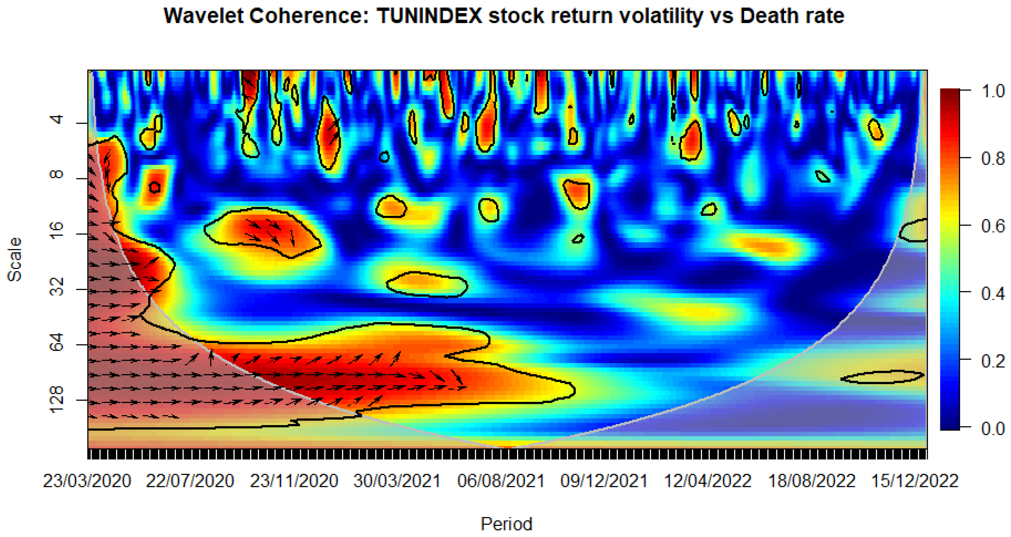
Globally, the COVID-19 virus persisted in causing anxiety, uncertainty, and distress in Tunisia. This situation heightened volatility in financial markets and led to liquidity challenges. The Tunisian stock market was not exempt from the profound effects of the COVID-19 outbreak, as evidenced by the ratios of confirmed cases and death cases, respectively (see Figure 2 and Figure 3).
Figure 2.
WAVELET TRANSFORM COHERENCE: Tunisian Stock return volatility versus COVID-19 cases rate. Notes: The black contour shows where the spectrum is significantly different from red noise at the 5% level. The lighter shade represents the cone of influence, marking high-power areas and indicating autocorrelation of wavelet power at each scale. The horizontal axis represents time from March 3rd, 2020, to December 30, 2022, and the vertical axis denotes scale bands with daily frequency. Arrows to the right (left) indicate in-phase (out-of-phase) relationships, meaning a positive (negative) connection. If arrows move right and up (down), the first variable "m" (Cases rate) drives (follows), while if arrows move left and up (down), variable "n" (TUNINDEX volatility) leads (lags). This visualization helps understand the dynamic relationships between variables. Source: The Author.
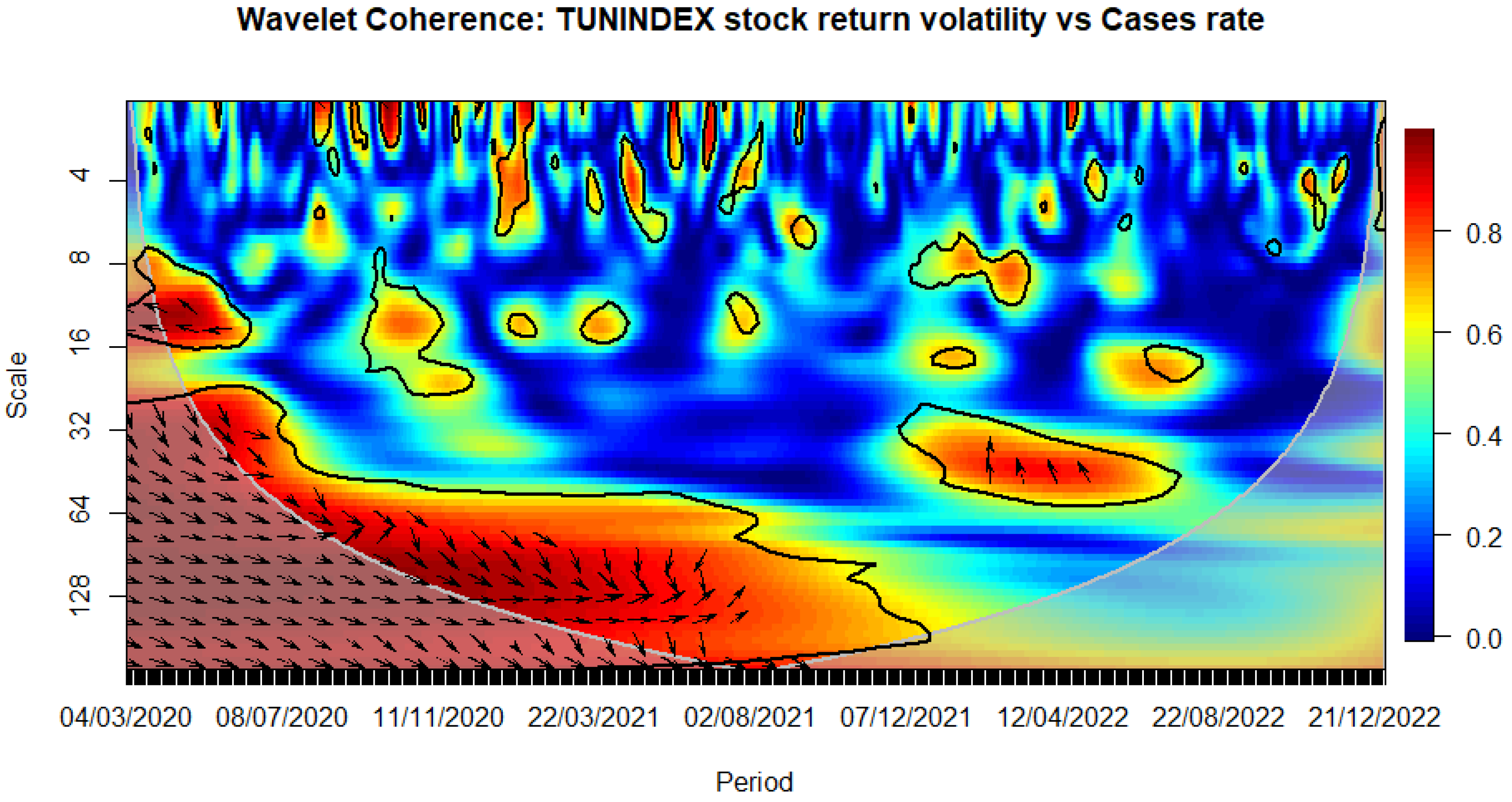
Figure 3.
WAVELET TRANSFORM COHERENCE: Tunisian stock Return volatility versus COVID-19 death rate. Notes: The black contour identifies areas where the spectrum is statistically significant at the 5% level compared to red noise. The lighter shade designates the cone of influence, outlining high-power regions. Time, ranging from March 23rd, 2020, to December 30, 2022, is represented on the horizontal axis, while the vertical axis denotes scale bands with daily frequency. Source: The Author.
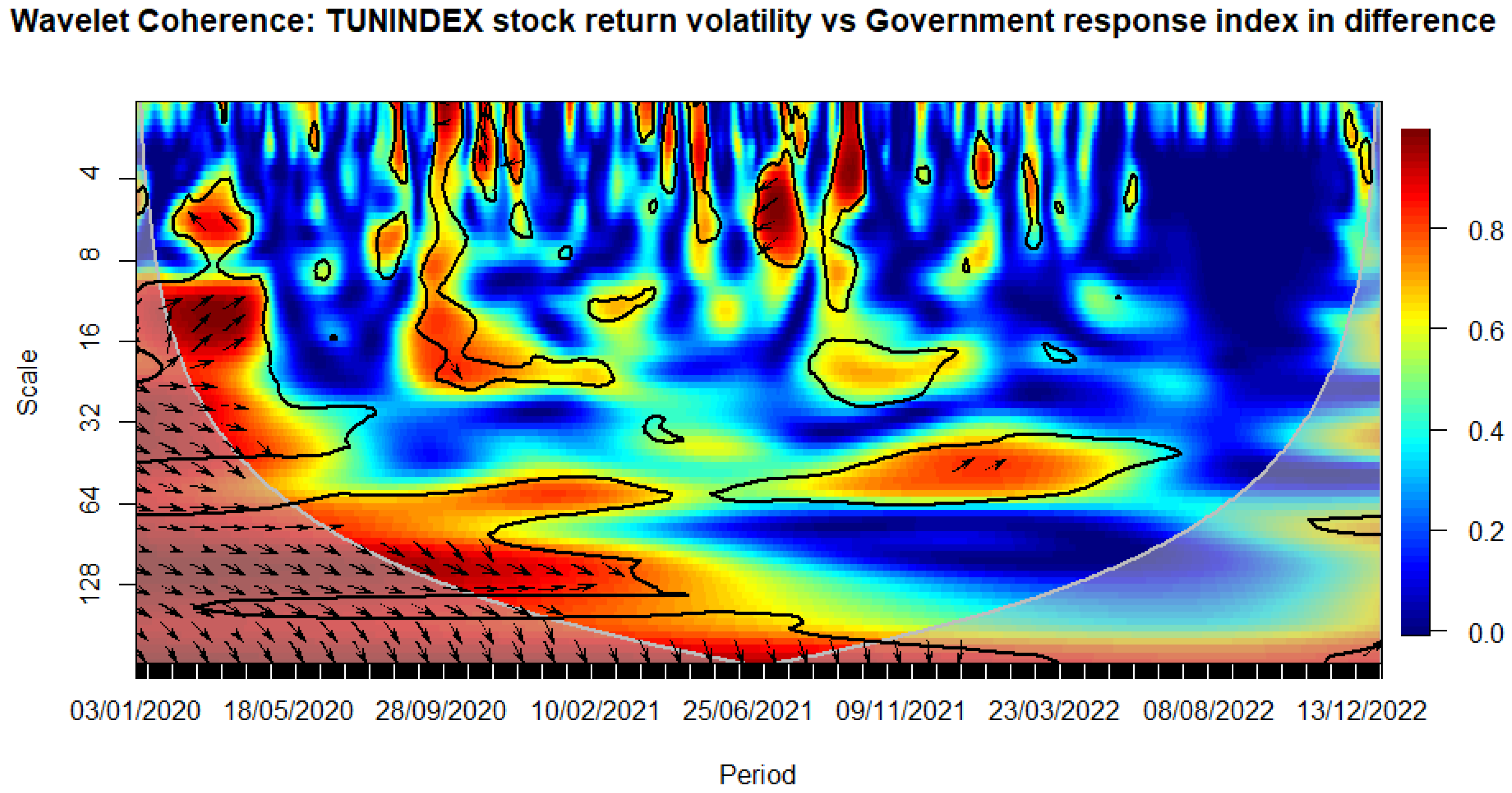
Among the government intervention metrics, the stringency index, the containment health index, and government response indices seem to affect the most stock market volatility during the COVID-19 times, while the economic support index had a neglected impact in the same period (see Figure 4, Figure 5, Figure 6 and Figure 7), confirming partially our previous results (see Table 4, Table 5, Table 6, Table 7, Table 8, Table 9, Table 10 and Table 11).
Now, we decompose the stringency index into sub-indices. Figure 8, Figure 9, Figure 10, Figure 11, Figure 12, Figure 13, Figure 14, Figure 15 and Figure 16 display the correlations between TUNINDEX stock market volatility and each of the nine-stringency index sub-indicators.
Figure 4.
WAVELET TRANSFORM COHERENCE: Tunisian stock return volatility versus Stringency index. Notes: The black contour identifies areas where the spectrum is statistically significant at the 5% level compared to red noise. The lighter shade designates the cone of influence, outlining high-power regions. Time, ranging from January 3rd, 2020, to December 30, 2022, is represented on the horizontal axis, while the vertical axis denotes scale bands with daily frequency. Source: The Author.
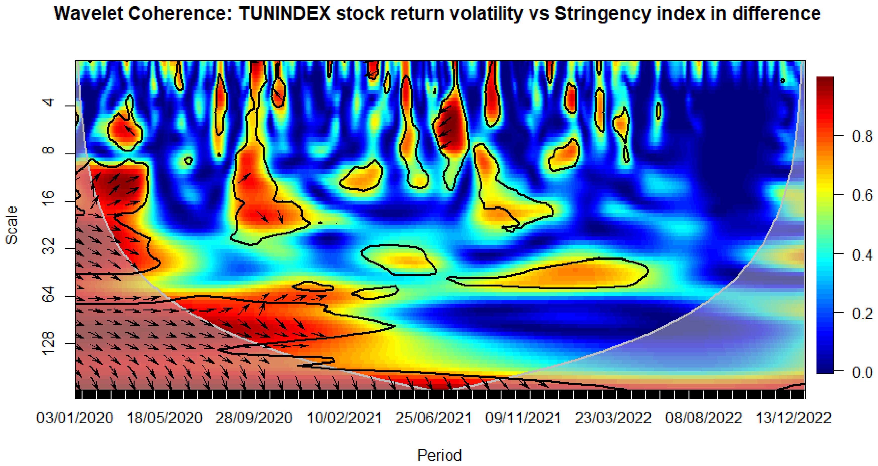
Figure 5.
WAVELET TRANSFORM COHERENCE: Tunisian stock return volatility versus Containment health index. Notes: The black contour identifies areas where the spectrum is statistically significant at the 5% level compared to red noise. The lighter shade designates the cone of influence, outlining high-power regions. Time, ranging from January 3rd, 2020, to December 30, 2022, is represented on the horizontal axis, while the vertical axis denotes scale bands with daily frequency. Source: The Author.
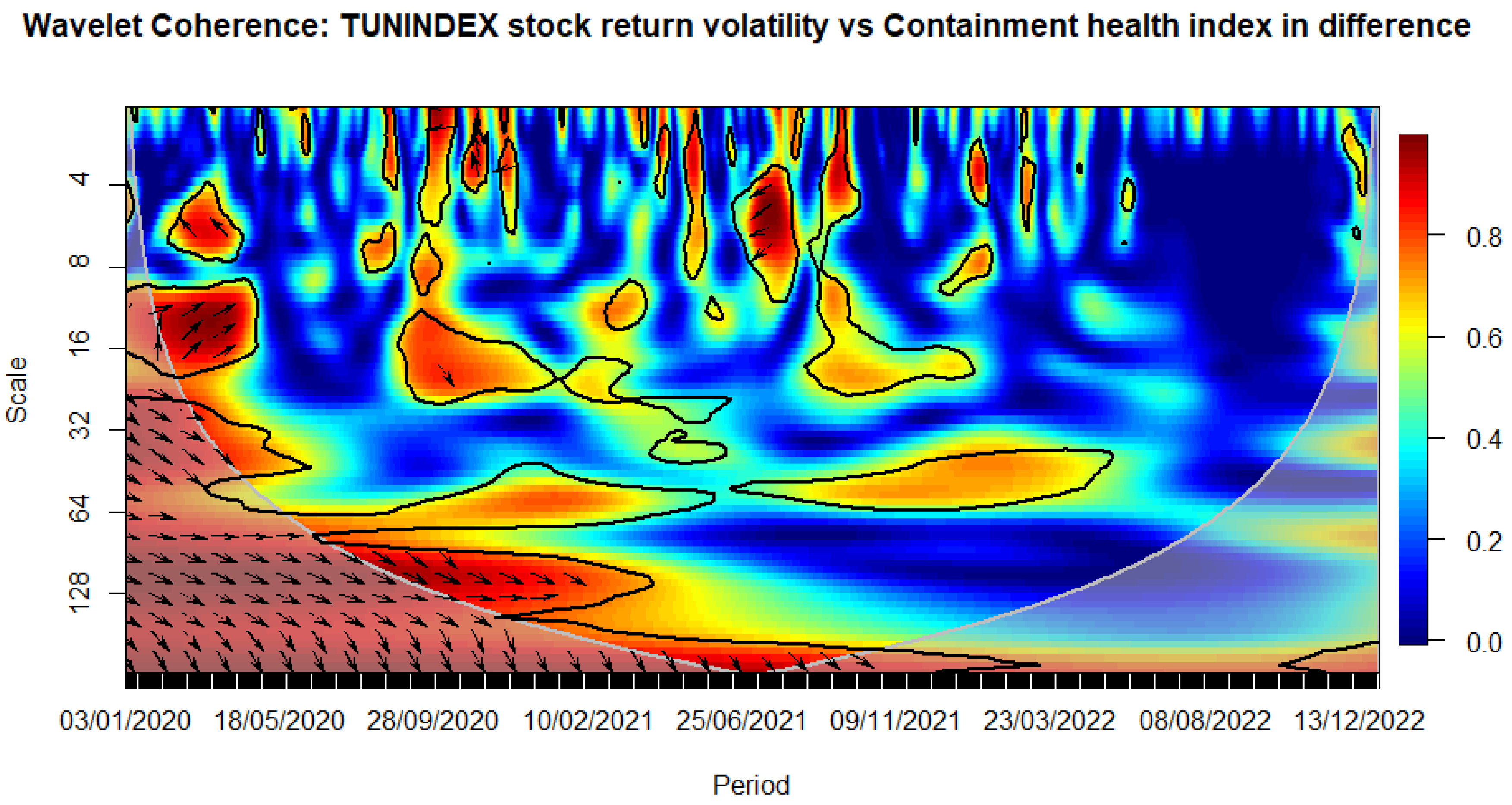
Figure 6.
WAVELET TRANSFORM COHERENCE: Tunisian stock return volatility versus Economic support index. Notes: The black contour identifies areas where the spectrum is statistically significant at the 5% level compared to red noise. The lighter shade designates the cone of influence, outlining high-power regions. Time, ranging from January 3rd, 2020, to December 30, 2022, is represented on the horizontal axis, while the vertical axis denotes scale bands with daily frequency. Source: The Author.
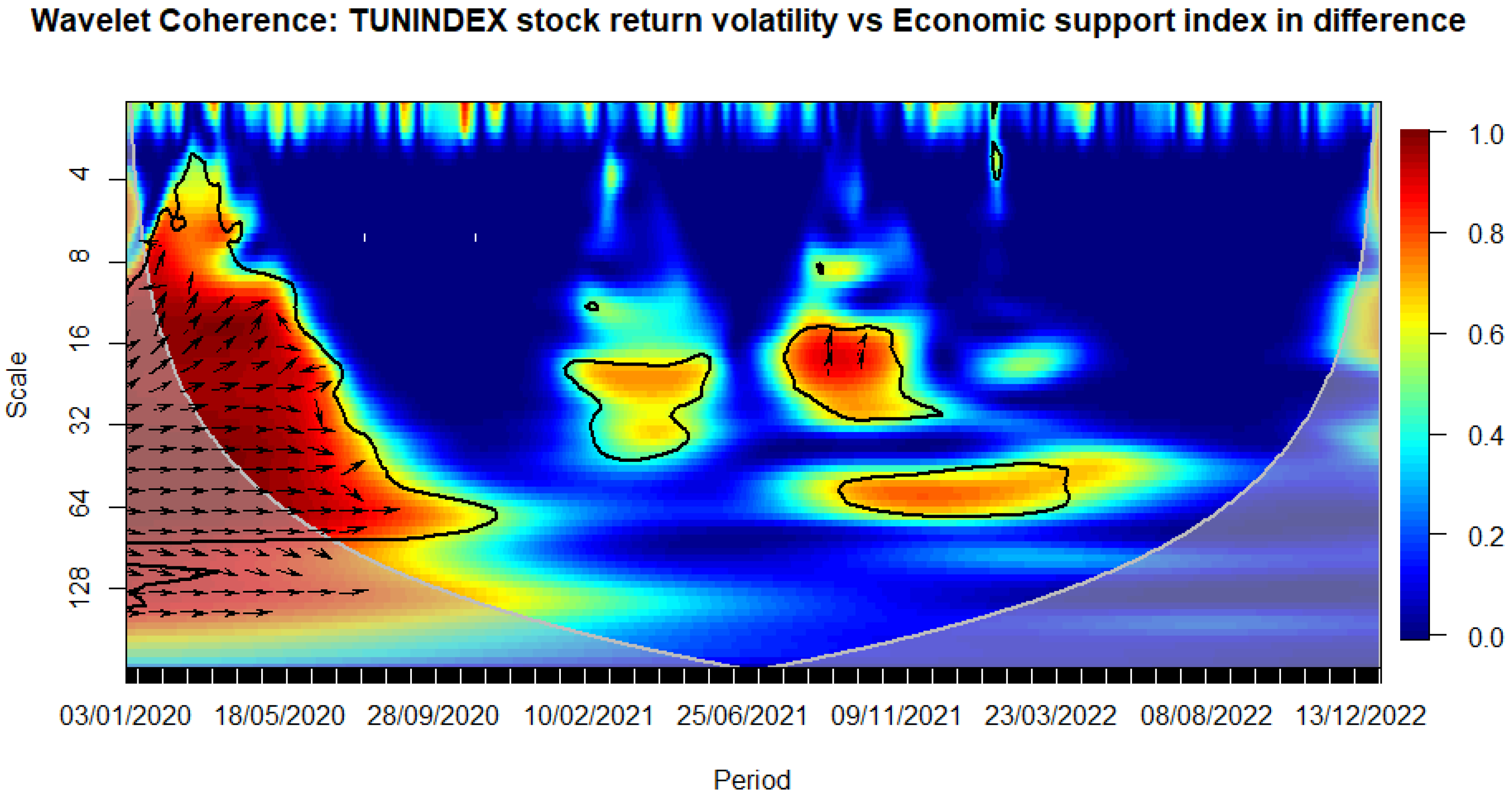
Figure 7.
Tunisian stock return volatility versus government response index. Notes: The black contour identifies areas where the spectrum is statistically significant at the 5% level compared to red noise. The lighter shade designates the cone of influence, outlining high-power regions. Time, ranging from January 3rd, 2020, to December 30, 2022, is represented on the horizontal axis, while the vertical axis denotes scale bands with daily frequency. Source: The Author.
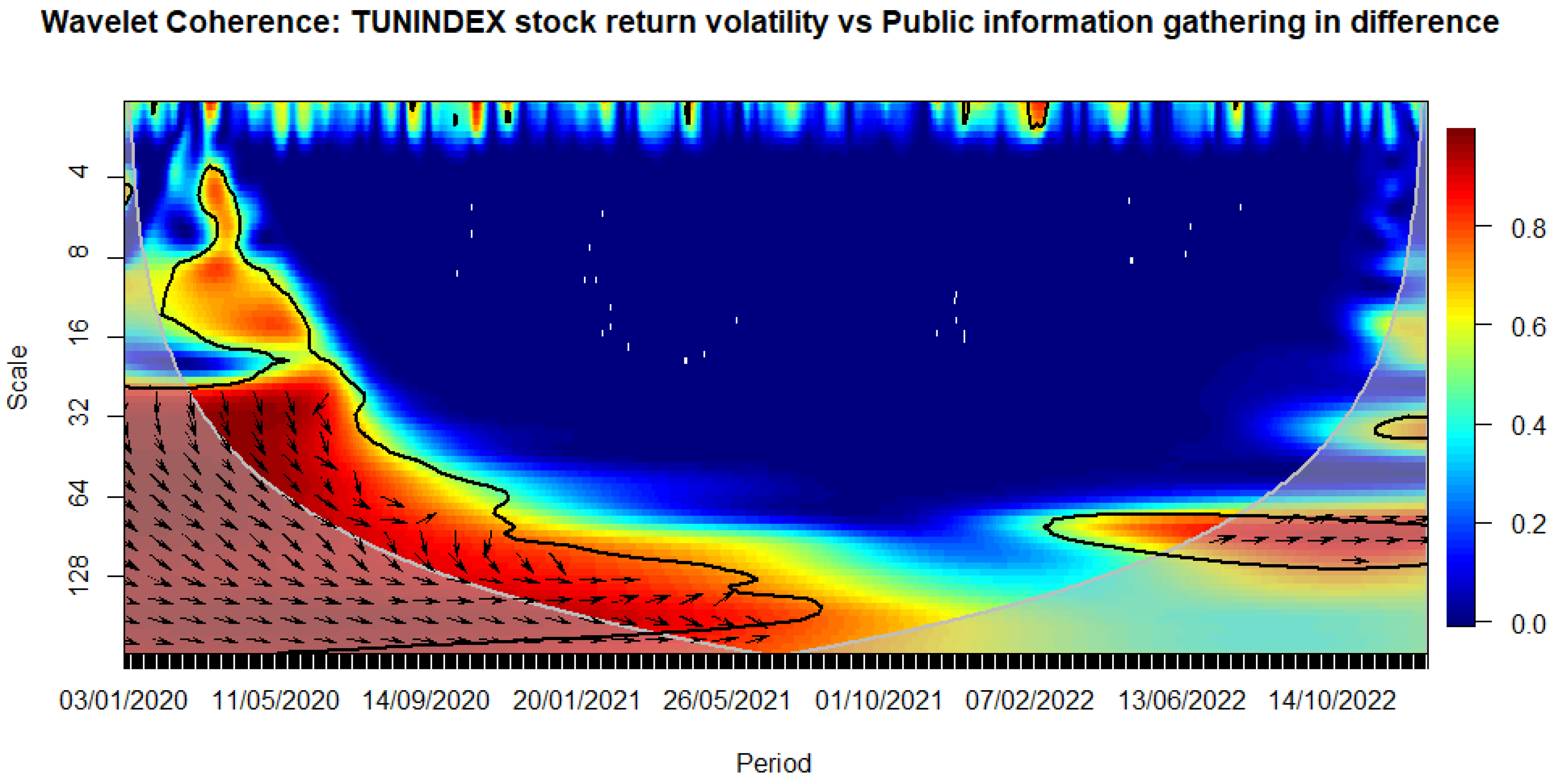
We observe that the closure of schools immediately influences volatility during the sanitary crisis (see Figure 8). Similarly, workplace closures exhibit an immediate impact, persisting over a medium-term horizon (see Figure 9). The cancellation of public events appears to have a notable and enduring impact over a longer-term horizon, as evidenced by a relatively high correlation with stock market volatility that persists beyond the COVID-19 period (see Figure 10). This pattern is evident when considering the stringency subindex related to restrictions on public gatherings (see Figure 11). Restrictions on public gatherings seem to impact conditional volatility over a short-term horizon (see Figure 12). Stay-at-home requirements distinctly impact volatility over short to medium-term horizons (see Figure 13). Restrictions on internal movements have an immediate impact on volatility triggered by the pandemic (see Figure 14). Control measures on international travel affect volatility over a medium-term horizon, with the effect extending post-COVID (see Figure 15). The gathering of public information influences volatility in the long run (see Figure 16).
The observed impact of various stringency measures on market volatility during the COVID-19 crisis holds significant implications for policymaking. Measures such as school closures and workplace shutdowns immediately contribute to volatility during the sanitary crisis, necessitating swift and targeted interventions to stabilize financial markets. Notably, workplace closures exhibit a sustained impact over a medium-term horizon, underscoring the importance of measures to counter prolonged market uncertainties. Public event cancellations demonstrate a lasting influence, emphasizing the need for strategies to manage and recover from enduring economic disruptions. The stringency subindex related to restrictions on public gatherings affects conditional volatility over a short-term horizon, requiring a delicate balance in policymaking to ensure public health measures without causing prolonged market disruptions. Stay-at-home requirements distinctly impact volatility over short to medium-term horizons, necessitating adaptive financial measures. Internal movement restrictions trigger an immediate market response, highlighting the importance of swift financial interventions. International travel control affects volatility over a medium-term horizon, prompting policymakers to consider strategies supporting industries reliant on international travel and trade. Lastly, the influence of public information gathering on long-term volatility underscores the importance of transparent communication for maintaining market stability. Policymakers can leverage these insights to design targeted interventions addressing both immediate and prolonged economic implications during crises.
Figure 8.
WAVELET TRANSFORM COHERENCE: Tunisian stock return versus School closing index. Notes: The black contour identifies areas where the spectrum is statistically significant at the 5% level compared to red noise. The lighter shade designates the cone of influence, outlining high-power regions. Time, ranging from January 3rd, 2020, to December 30, 2022, is represented on the horizontal axis, while the vertical axis denotes scale bands with daily frequency. Source: The Author.
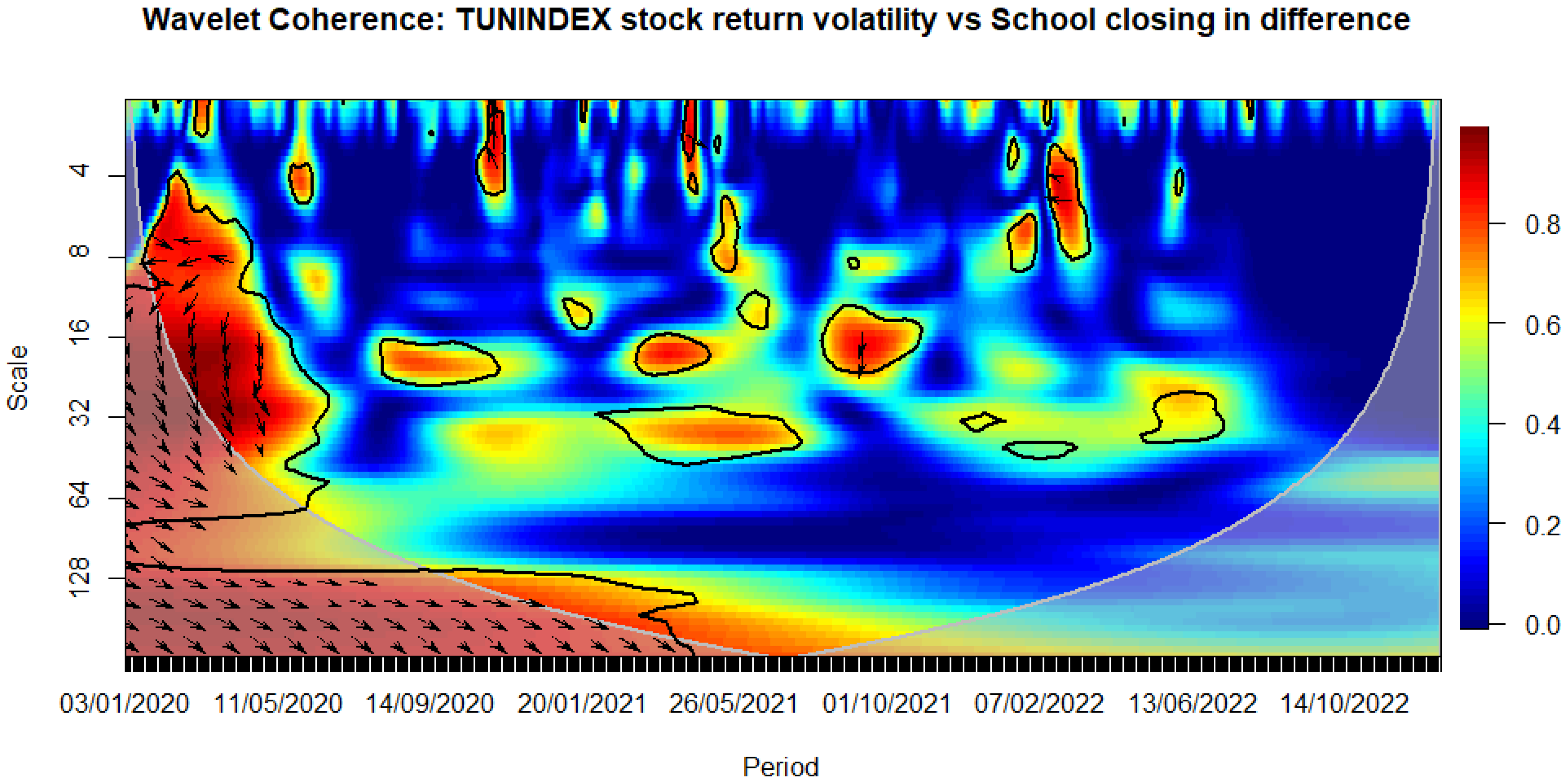
Figure 9.
WAVELET TRANSFORM COHERENCE: Tunisian stock return versus Workplace closing. Notes: The black contour identifies areas where the spectrum is statistically significant at the 5% level compared to red noise. The lighter shade designates the cone of influence, outlining high-power regions. Time, ranging from January 3rd, 2020, to December 30, 2022, is represented on the horizontal axis, while the vertical axis denotes scale bands with daily frequency. Source: The Author.
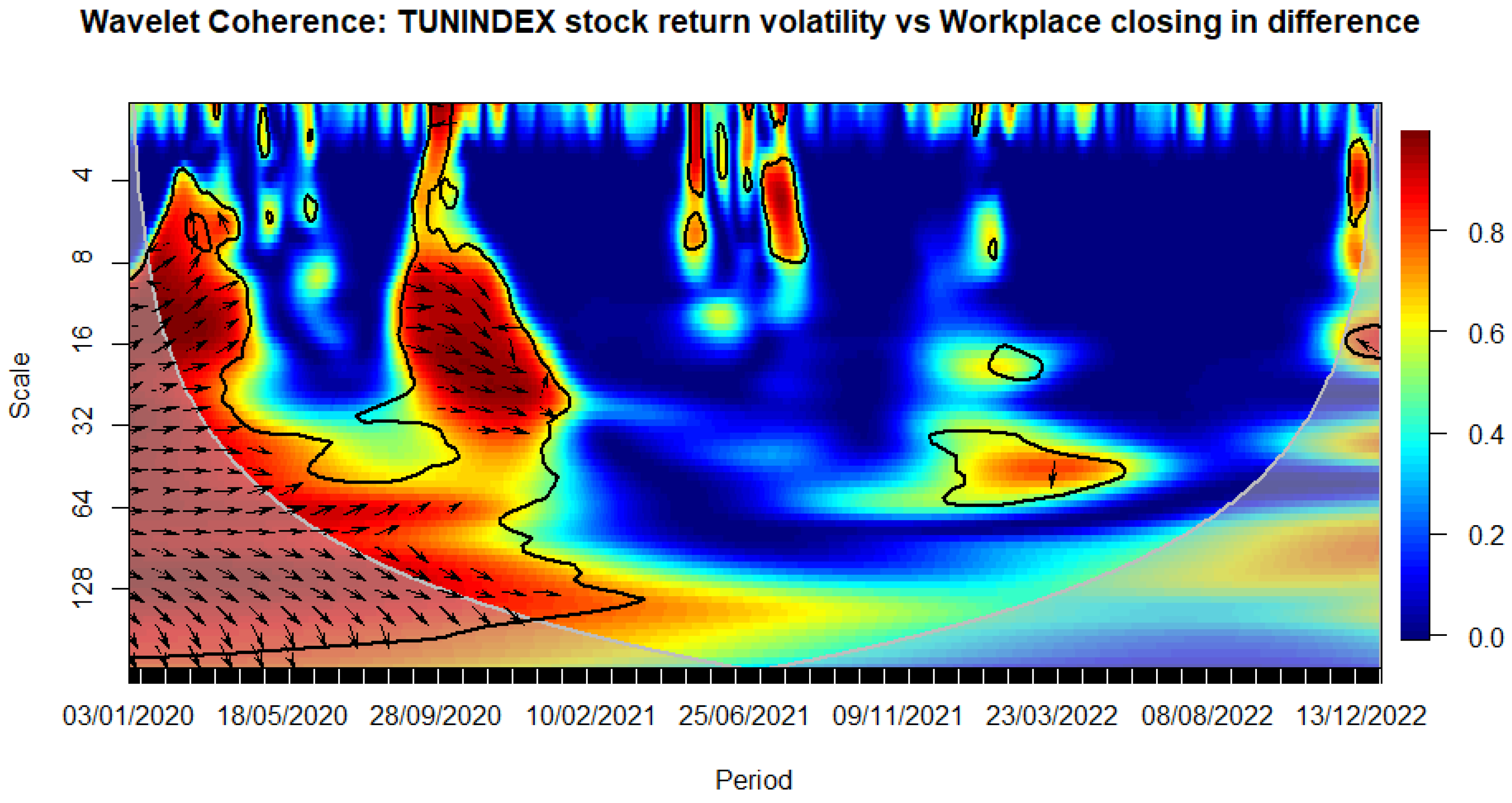
Figure 10.
WAVELET TRANSFORM COHERENCE: Tunisian stock return versus Public events canceling. Notes: The black contour identifies areas where the spectrum is statistically significant at the 5% level compared to red noise. The lighter shade designates the cone of influence, outlining high-power regions. Time, ranging from January 3rd, 2020, to December 30, 2022, is represented on the horizontal axis, while the vertical axis denotes scale bands with daily frequency. Source: The Author.
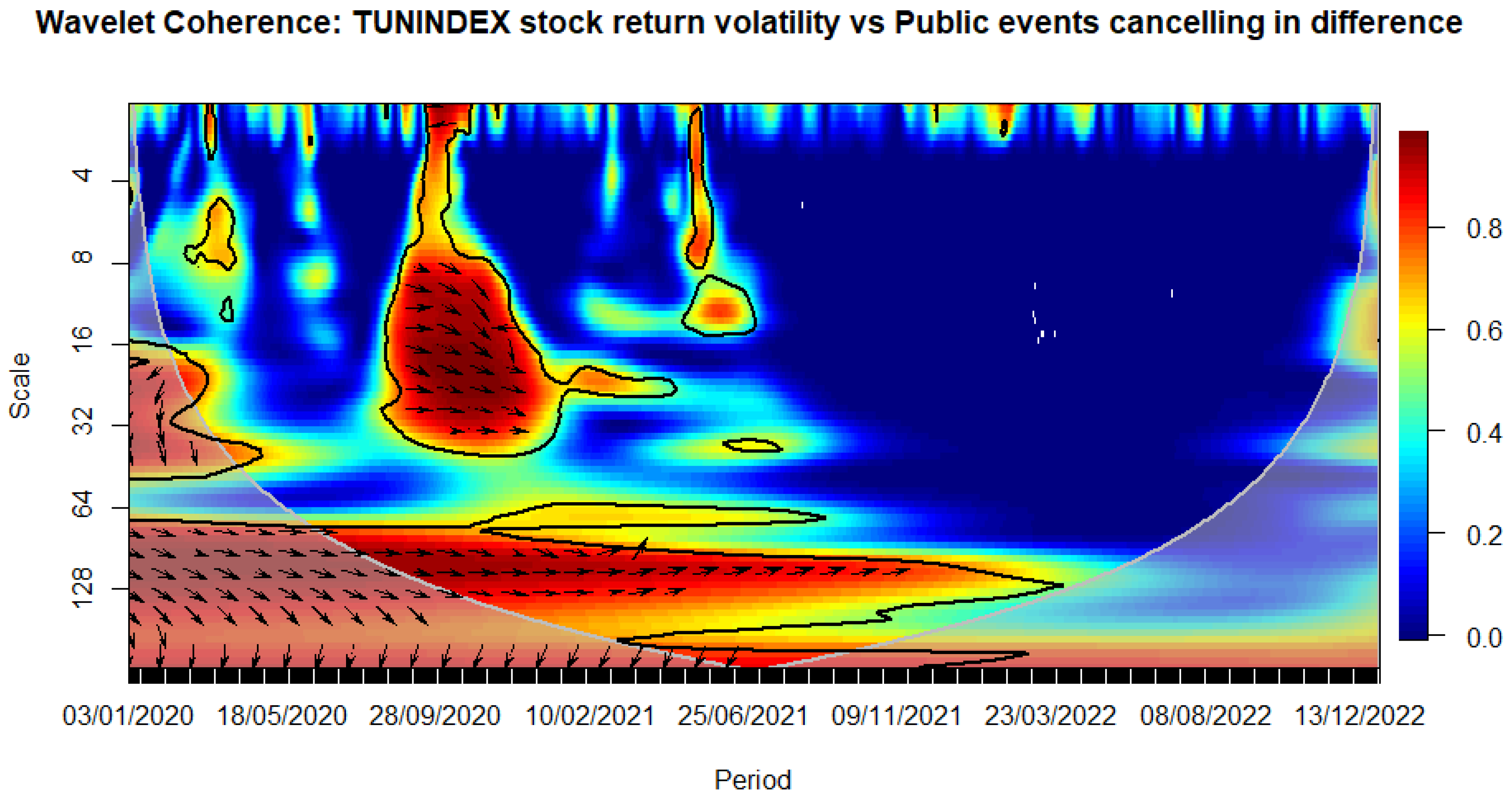
Figure 11.
WAVELET TRANSFORM COHERENCE: Tunisian stock return versus Public gathering restrictions. Notes: The black contour identifies areas where the spectrum is statistically significant at the 5% level compared to red noise. The lighter shade designates the cone of influence, outlining high-power regions. Time, ranging from January 3rd, 2020, to December 30, 2022, is represented on the horizontal axis, while the vertical axis denotes scale bands with daily frequency. Source: The Author.
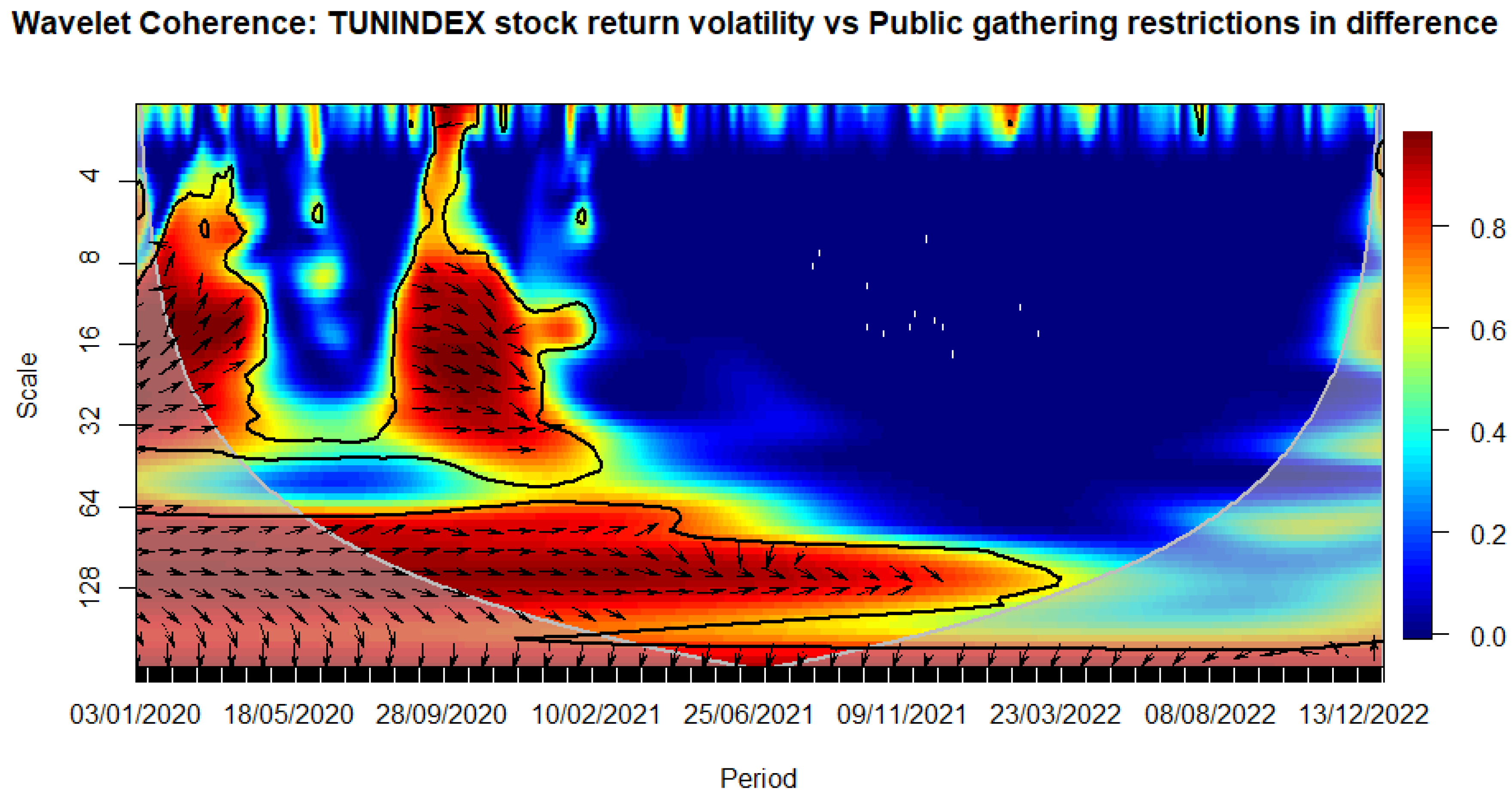
Figure 12.
WAVELET TRANSFORM COHERENCE: Tunisian stock return versus Public transport closure. Notes: The black contour identifies areas where the spectrum is statistically significant at the 5% level compared to red noise. The lighter shade designates the cone of influence, outlining high-power regions. Time, ranging from January 3rd, 2020, to December 30, 2022, is represented on the horizontal axis, while the vertical axis denotes scale bands with daily frequency. Source: The Author.
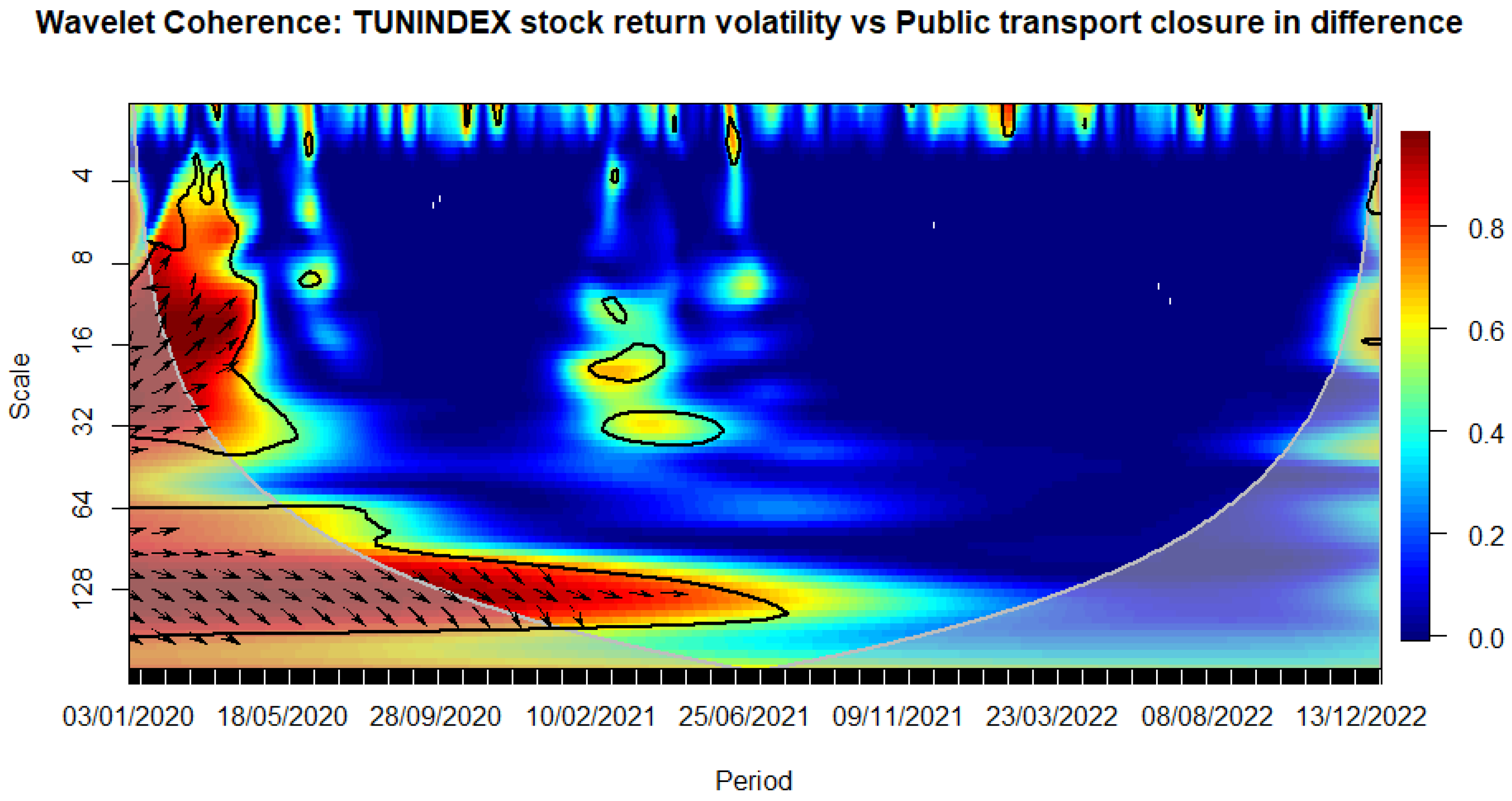
Figure 13.
WAVELET TRANSFORM COHERENCE: Tunisian stock return versus Stay-at-home requirements. Notes: The black contour identifies areas where the spectrum is statistically significant at the 5% level compared to red noise. The lighter shade designates the cone of influence, outlining high-power regions. Time, ranging from January 3rd, 2020, to December 30, 2022, is represented on the horizontal axis, while the vertical axis denotes scale bands with daily frequency. Source: The Author.
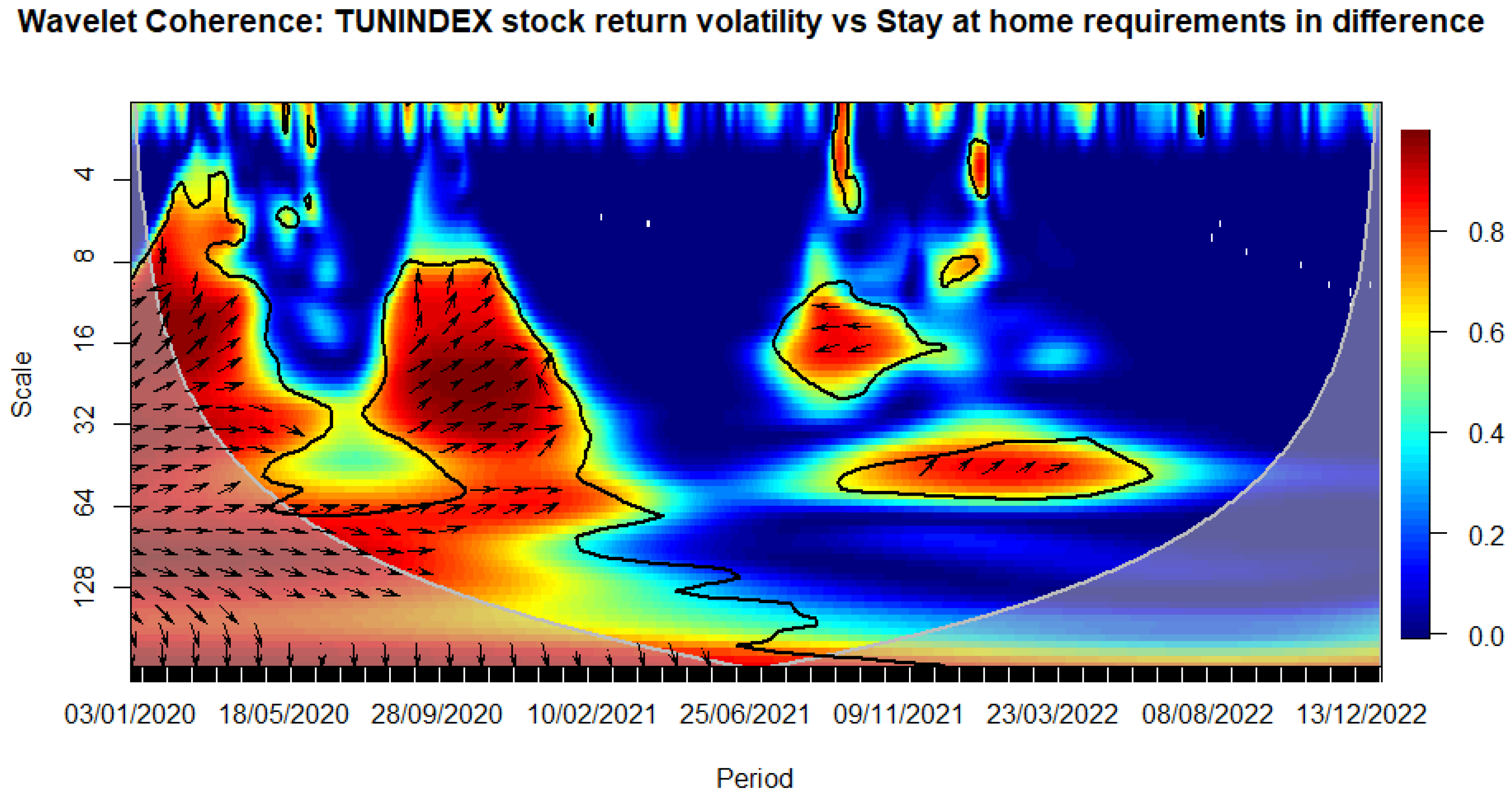
Figure 14.
WAVELET TRANSFORM COHERENCE: Tunisian stock return versus Internal movements restrictions Notes: The black contour identifies areas where the spectrum is statistically significant at the 5% level compared to red noise. The lighter shade designates the cone of influence, outlining high-power regions. Time, ranging from January 3rd, 2020, to December 30, 2022, is represented on the horizontal axis, while the vertical axis denotes scale bands with daily frequency. Source: The Author.
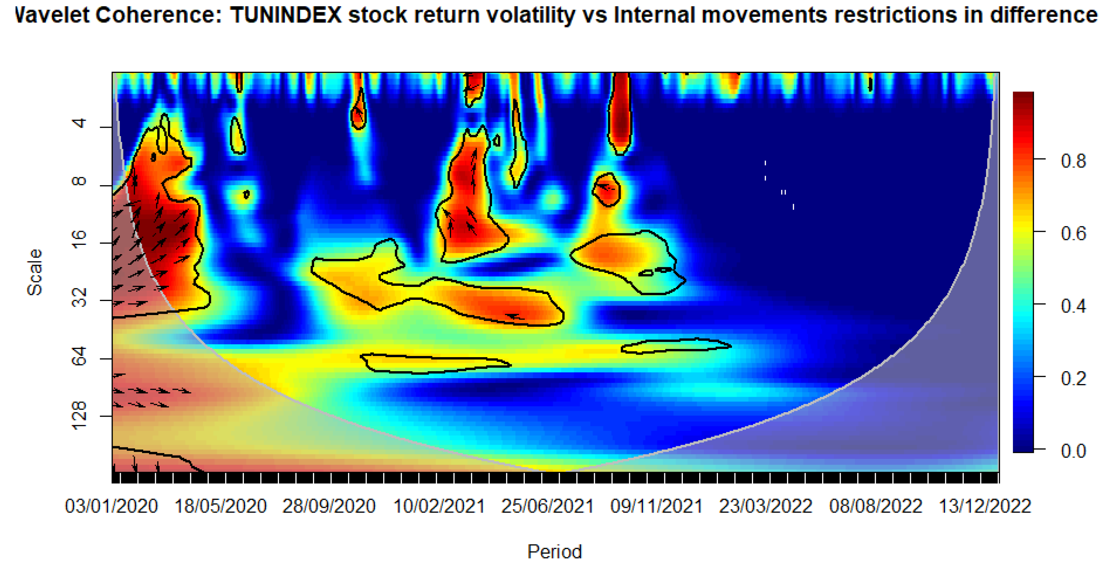
Figure 15.
WAVELET TRANSFORM COHERENCE: Tunisian stock return versus International travel control. Notes: The black contour identifies areas where the spectrum is statistically significant at the 5% level compared to red noise. The lighter shade designates the cone of influence, outlining high-power regions. Time, ranging from January 3rd, 2020, to December 30, 2022, is represented on the horizontal axis, while the vertical axis denotes scale bands with daily frequency. Source: The Author.
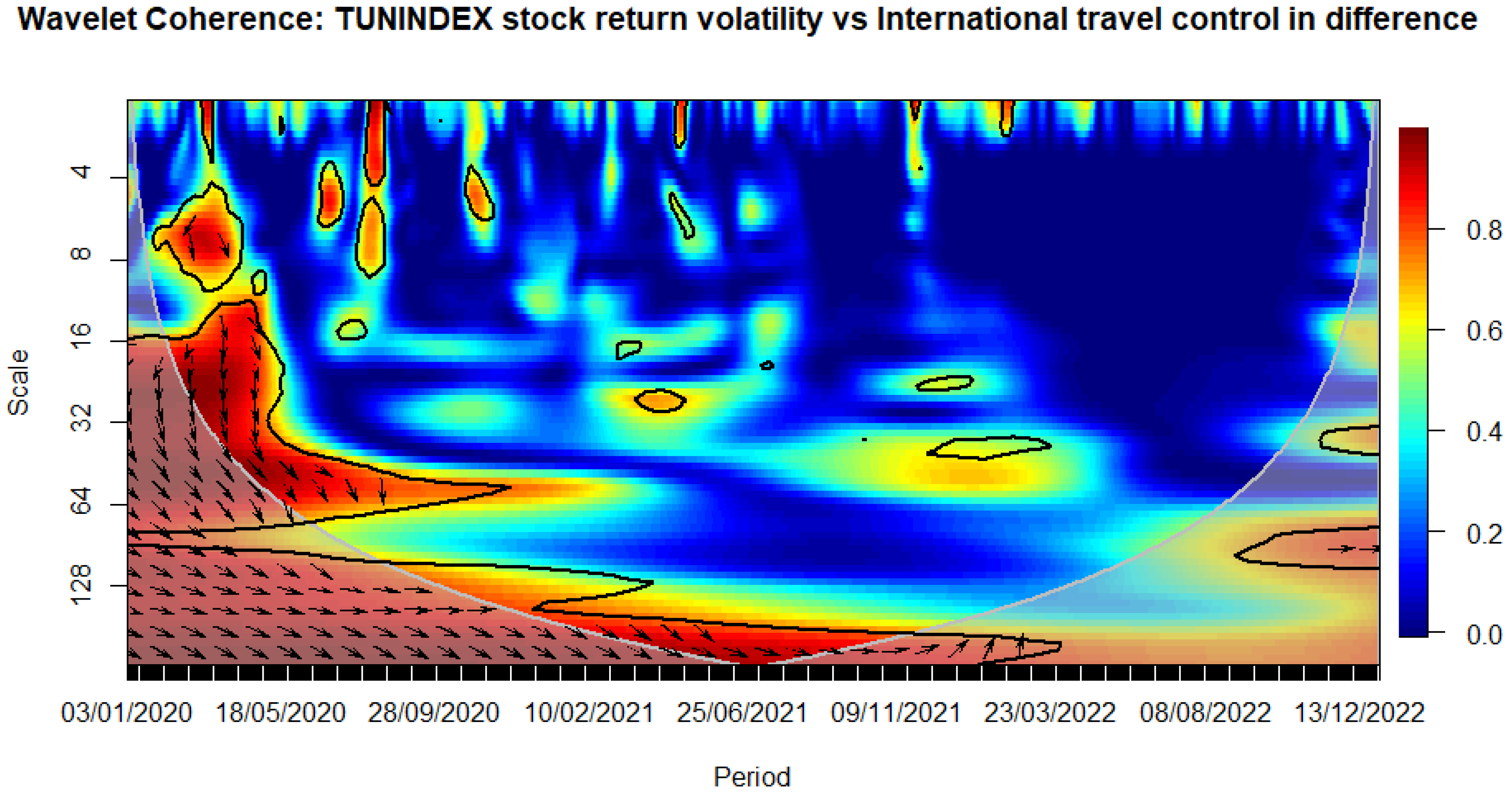
Figure 16.
WAVELET TRANSFORM COHERENCE: Tunisian stock return versus Public information gathering. Notes: The black contour identifies areas where the spectrum is statistically significant at the 5% level compared to red noise. The lighter shade designates the cone of influence, outlining high-power regions. Time, ranging from January 3rd, 2020, to December 30, 2022, is represented on the horizontal axis, while the vertical axis denotes scale bands with daily frequency. Source: The Author.
4.3. Impact of uncertainty on the TUNINDEX stock return volatility using ARDL
The earlier COVID-19 and government intervention metrics serve as indicators of the broader economic and health landscape, influencing investor confidence and risk perceptions. However, the uncertainty surrounding COVID-19 has a notable impact on stock market volatility. The dataset comprises daily values of Economic Policy Uncertainty (EPU), the Infectious Disease EMV Tracker (IDEMV), Implied Volatility (VIX), and US Equity Market Uncertainty (EMU). The development of EPU and IDEMV was initiated by Baker et al. (2016, 2019). Quoting Tissaoui et al. (2022, p. 4), EPU quantifies the number of articles in major newspapers covering news related to the economy, uncertainty, monetary and trade policies, and financial regulation in the US (https://www.policyuncertainty.com/us_monthly.html). IDEMV (https://www.policyuncertainty.com/infectious_EMV.html). Additionally, the VIX is the implied volatility index of the Chicago Board Options Exchange. We gather data on EMU from the Federal Reserve Bank of St. Louis https://fred.stlouisfed.org/series/WLEMUINDXD. Unit root and Johansen tests indicate that the variables are I(0) and I(1) and cointegrated (see Table 12 and Table 13, respectively). We adjust coefficients to the White estimator as only heteroscedasticity is detected when analyzing residuals that remain uncorrelated and stable according to the Ramsey test (not shown for tractable reasons but available upon request). All variables, except EPU, have both positive long and short-term effects on Tunisian stock market volatility (see Table 14). This could be due to factors like the stronger influence of local economic conditions, political stability, and industry-specific dynamics on TUNINDEX volatility. At the same time, the findings emphasize the importance of monitoring not only domestic factors but also global economic and health-related developments to anticipate and navigate volatility in the Tunisian stock market.
Table 12.
Unit root test results.
| UNIT ROOT TEST TABLE (PP) | ||||||
| At Level | ||||||
| CONDVAR_TUN | EMU | EPU | IMEDV | VIX | ||
| With Constant | t-Statistic | -5.8831 | -17.7598 | -9.9104 | -16.6159 | -3.8380 |
| Prob. | 0.0000 | 0.0000 | 0.0000 | 0.0000 | 0.0027 | |
| *** | *** | *** | *** | *** | ||
| With Constant & Trend | t-Statistic | -6.0788 | -18.5316 | -12.8521 | -17.9677 | -4.0035 |
| Prob. | 0.0000 | 0.0000 | 0.0000 | 0.0000 | 0.0090 | |
| *** | *** | *** | *** | *** | ||
| Without Constant & Trend | t-Statistic | -4.9680 | -8.6348 | -2.8802 | -6.0788 | -1.0620 |
| Prob. | 0.0000 | 0.0000 | 0.0039 | 0.0000 | 0.2607 | |
| *** | *** | *** | *** | n0 | ||
| At First Difference | ||||||
| d(CONDVAR_TUN) | d(EMU) | d(EPU) | d(IMEDV) | d(VIX) | ||
| With Constant | t-Statistic | -23.6448 | -325.2894 | -72.6030 | -104.2793 | -34.4302 |
| Prob. | 0.0000 | 0.0001 | 0.0001 | 0.0001 | 0.0000 | |
| *** | *** | *** | *** | *** | ||
| With Constant & Trend | t-Statistic | -23.6141 | -321.7941 | -72.7563 | -105.3697 | -34.4139 |
| Prob. | 0.0000 | 0.0001 | 0.0001 | 0.0001 | 0.0000 | |
| *** | *** | *** | *** | *** | ||
| Without Constant & Trend | t-Statistic | -23.6785 | -330.9807 | -72.6602 | -104.4676 | -34.4538 |
| Prob. | 0.0000 | 0.0001 | 0.0001 | 0.0001 | 0.0000 | |
| *** | *** | *** | *** | *** | ||
| UNIT ROOT TEST TABLE (ADF) | ||||||
| At Level | ||||||
| CONDVAR_TUN | EMU | EPU | IMEDV | VIX | ||
| With Constant | t-Statistic | -6.6410 | -4.9317 | -2.9816 | -4.5133 | -3.5374 |
| Prob. | 0.0000 | 0.0000 | 0.0371 | 0.0002 | 0.0073 | |
| *** | *** | ** | *** | *** | ||
| With Constant & Trend | t-Statistic | -6.9345 | -5.2977 | -3.8321 | -5.2213 | -3.6962 |
| Prob. | 0.0000 | 0.0001 | 0.0154 | 0.0001 | 0.0232 | |
| *** | *** | ** | *** | ** | ||
| Without Constant & Trend | t-Statistic | -5.5114 | -2.2028 | -1.4589 | -2.1077 | -0.9997 |
| Prob. | 0.0000 | 0.0267 | 0.1352 | 0.0338 | 0.2850 | |
| *** | ** | n0 | ** | n0 | ||
| At First Difference | ||||||
| d(CONDVAR_TUN) | d(EMU) | d(EPU) | d(IMEDV) | d(VIX) | ||
| With Constant | t-Statistic | -12.8719 | -17.3275 | -20.8561 | -21.3098 | -14.0249 |
| Prob. | 0.0000 | 0.0000 | 0.0000 | 0.0000 | 0.0000 | |
| *** | *** | *** | *** | *** | ||
| With Constant & Trend | t-Statistic | -12.8629 | -17.3155 | -20.8449 | -21.2986 | -14.0230 |
| Prob. | 0.0000 | 0.0000 | 0.0000 | 0.0000 | 0.0000 | |
| *** | *** | *** | *** | *** | ||
| Without Constant & Trend | t-Statistic | -12.8813 | -17.3398 | -20.8711 | -21.3238 | -14.0341 |
| Prob. | 0.0000 | 0.0000 | 0.0000 | 0.0000 | 0.0000 | |
| *** | *** | *** | *** | *** | ||
* MacKinnon (1996) one-sided p-values.
Table 13.
Johansen cointegration test.
| Date: 01/12/24 Time: 16:39 | ||||
| Sample (adjusted): 1/10/2020 12/30/2022 | ||||
| Included observations: 693 after adjustments | ||||
| Trend assumption: Linear deterministic trend | ||||
| Series: EMU EPU VIX IMEDV CONDVAR_TUN | ||||
| Lags interval (in first differences): 1 to 4 | ||||
| Unrestricted Cointegration Rank Test (Trace) | ||||
| Hypothesized | Trace | 0.05 | ||
| No. of CE(s) | Eigenvalue | Statistic | Critical Value | Prob.** |
| None * | 0.159673 | 287.2357 | 69.81889 | 0.0001 |
| At most 1 * | 0.087501 | 166.6788 | 47.85613 | 0.0000 |
| At most 2 * | 0.074215 | 103.2221 | 29.79707 | 0.0000 |
| At most 3 * | 0.048996 | 49.78261 | 15.49471 | 0.0000 |
| At most 4 * | 0.021368 | 14.96863 | 3.841466 | 0.0001 |
| Trace test indicates 5 cointegrating eqn(s) at the 0.05 level | ||||
| * denotes rejection of the hypothesis at the 0.05 level | ||||
| ** MacKinnon-Haug-Michelis (1999) p-values | ||||
Table 14.
Long-run and short-run results of ARDL.
| Using EPU and VIX | Levels Equation | ||||
| Case 2: Restricted Constant and No Trend | |||||
| Variable | Coefficient | Std. Error | t-Statistic | Prob. | |
| EPU | -1.10E-08 | 2.72E-08 | -0.406081 | 0.6848 | |
| VIX | 2.44E-06 | 9.45E-07 | 2.576858 | 0.0102 | |
| C | -4.02E-05 | 1.99E-05 | -2.022307 | 0.0435 | |
| EC = CONDVAR_TUN - (-0.0000*EPU + 0.0000*VIX -0.0000 ) | |||||
| F-Bounds Test | Null Hypothesis: No levels of relationship | ||||
| Test Statistic | Value | Signif. | I(0) | I(1) | |
| Asymptotic: n=1000 | |||||
| F-statistic | 20.22501 | 10% | 2.63 | 3.35 | |
| k | 2 | 5% | 3.1 | 3.87 | |
| 2.5% | 3.55 | 4.38 | |||
| 1% | 4.13 | 5 | |||
| ECM Regression | |||||
| Case 2: Restricted Constant and No Trend | |||||
| Variable | Coefficient | Std. Error | t-Statistic | Prob. | |
| D(CONDVAR_TUN(-1)) | 0.305200 | 0.036072 | 8.460905 | 0.0000 | |
| D(CONDVAR_TUN(-2)) | 0.163597 | 0.037889 | 4.317848 | 0.0000 | |
| D(CONDVAR_TUN(-3)) | -0.135407 | 0.038054 | -3.558262 | 0.0004 | |
| D(CONDVAR_TUN(-4)) | 0.042966 | 0.036567 | 1.174983 | 0.2404 | |
| D(CONDVAR_TUN(-5)) | 0.156755 | 0.036535 | 4.290596 | 0.0000 | |
| D(CONDVAR_TUN(-6)) | -0.064229 | 0.036672 | -1.751465 | 0.0803 | |
| D(VIX) | 4.99E-07 | 1.75E-07 | 2.846085 | 0.0046 | |
| D(VIX(-1)) | 5.59E-07 | 1.83E-07 | 3.060780 | 0.0023 | |
| CointEq(-1)* | -0.214080 | 0.023749 | -9.014119 | 0.0000 | |
| Using EMU + VIX | Levels Equation | ||||
| Case 2: Restricted Constant and No Trend | |||||
| Variable | Coefficient | Std. Error | t-Statistic | Prob. | |
| EMU | 1.02E-07 | 5.16E-08 | 1.982838 | 0.0478 | |
| VIX | 1.33E-06 | 5.94E-07 | 2.233982 | 0.0258 | |
| C | -2.63E-05 | 1.49E-05 | -1.769359 | 0.0773 | |
| EC = CONDVAR_TUN - (0.0000*EMU + 0.0000*VIX -0.0000 ) | |||||
| F-Bounds Test | Null Hypothesis: No levels relationship | ||||
| Test Statistic | Value | Signif. | I(0) | I(1) | |
| Asymptotic: n=1000 | |||||
| F-statistic | 16.68016 | 10% | 2.63 | 3.35 | |
| k | 2 | 5% | 3.1 | 3.87 | |
| 2.5% | 3.55 | 4.38 | |||
| 1% | 4.13 | 5 | |||
| ECM Regression | |||||
| Case 2: Restricted Constant and No Trend | |||||
| Variable | Coefficient | Std. Error | t-Statistic | Prob. | |
| D(CONDVAR_TUN(-1)) | 0.280360 | 0.037720 | 7.432660 | 0.0000 | |
| D(CONDVAR_TUN(-2)) | 0.169588 | 0.039402 | 4.303995 | 0.0000 | |
| D(CONDVAR_TUN(-3)) | -0.147548 | 0.039403 | -3.744638 | 0.0002 | |
| D(CONDVAR_TUN(-4)) | 0.033769 | 0.037466 | 0.901324 | 0.3677 | |
| D(CONDVAR_TUN(-5)) | 0.153700 | 0.037312 | 4.119377 | 0.0000 | |
| D(CONDVAR_TUN(-6)) | -0.080614 | 0.037319 | -2.160150 | 0.0311 | |
| D(EMU) | -5.65E-09 | 6.22E-09 | -0.908323 | 0.3640 | |
| D(EMU(-1)) | -2.82E-08 | 7.75E-09 | -3.638482 | 0.0003 | |
| D(EMU(-2)) | -2.49E-08 | 8.39E-09 | -2.968032 | 0.0031 | |
| D(EMU(-3)) | -3.79E-08 | 8.57E-09 | -4.418311 | 0.0000 | |
| D(EMU(-4)) | -2.99E-08 | 8.34E-09 | -3.587680 | 0.0004 | |
| D(EMU(-5)) | -3.58E-09 | 7.60E-09 | -0.471456 | 0.6375 | |
| D(EMU(-6)) | 1.44E-08 | 6.23E-09 | 2.315235 | 0.0209 | |
| D(VIX) | 4.39E-07 | 1.75E-07 | 2.513163 | 0.0122 | |
| D(VIX(-1)) | 7.64E-07 | 1.87E-07 | 4.091321 | 0.0000 | |
| D(VIX(-2)) | 3.64E-07 | 1.88E-07 | 1.933189 | 0.0536 | |
| D(VIX(-3)) | 4.45E-07 | 1.89E-07 | 2.355937 | 0.0188 | |
| D(VIX(-4)) | 2.90E-07 | 1.90E-07 | 1.523589 | 0.1281 | |
| D(VIX(-5)) | 2.81E-07 | 1.89E-07 | 1.489922 | 0.1367 | |
| D(VIX(-6)) | 4.49E-07 | 1.80E-07 | 2.488358 | 0.0131 | |
| CointEq(-1)* | -0.208323 | 0.025447 | -8.186456 | 0.0000 | |
| Using IDEMV + VIX | Levels Equation | ||||
| Case 2: Restricted Constant and No Trend | |||||
| Variable | Coefficient | Std. Error | t-Statistic | Prob. | |
| IMEDV | 7.74E-07 | 3.47E-07 | 2.230579 | 0.0260 | |
| VIX | 1.56E-06 | 6.78E-07 | 2.293725 | 0.0221 | |
| C | -3.15E-05 | 1.69E-05 | -1.860152 | 0.0633 | |
| EC = CONDVAR_TUN - (0.0000*IMEDV + 0.0000*VIX -0.0000 ) | |||||
| F-Bounds Test | Null Hypothesis: No levels relationship | ||||
| Test Statistic | Value | Signif. | I(0) | I(1) | |
| Asymptotic: n=1000 | |||||
| F-statistic | 16.16596 | 10% | 2.63 | 3.35 | |
| k | 2 | 5% | 3.1 | 3.87 | |
| 2.5% | 3.55 | 4.38 | |||
| 1% | 4.13 | 5 | |||
| ECM Regression | |||||
| Case 2: Restricted Constant and No Trend | |||||
| Variable | Coefficient | Std. Error | t-Statistic | Prob. | |
| D(CONDVAR_TUN(-1)) | 0.294640 | 0.038541 | 7.644852 | 0.0000 | |
| D(CONDVAR_TUN(-2)) | 0.156728 | 0.040128 | 3.905726 | 0.0001 | |
| D(CONDVAR_TUN(-3)) | -0.148119 | 0.039993 | -3.703629 | 0.0002 | |
| D(CONDVAR_TUN(-4)) | 0.032052 | 0.037988 | 0.843737 | 0.3991 | |
| D(CONDVAR_TUN(-5)) | 0.149479 | 0.037947 | 3.939136 | 0.0001 | |
| D(CONDVAR_TUN(-6)) | -0.066308 | 0.037763 | -1.755902 | 0.0796 | |
| D(IMEDV) | 4.17E-08 | 6.49E-08 | 0.642959 | 0.5205 | |
| D(IDEMV(-1)) | -1.54E-07 | 8.11E-08 | -1.893384 | 0.0587 | |
| D(IDEMV(-2)) | -1.26E-07 | 8.97E-08 | -1.409433 | 0.1592 | |
| D(IDEMV(-3)) | -1.98E-07 | 9.24E-08 | -2.139318 | 0.0328 | |
| D(IDEMV(-4)) | -1.67E-07 | 8.99E-08 | -1.854306 | 0.0641 | |
| D(IDEMV(-5)) | -5.06E-08 | 8.15E-08 | -0.620560 | 0.5351 | |
| D(IDEMV(-6)) | 1.28E-07 | 6.64E-08 | 1.925914 | 0.0545 | |
| D(VIX) | 4.08E-07 | 1.81E-07 | 2.259421 | 0.0242 | |
| D(VIX(-1)) | 7.04E-07 | 1.95E-07 | 3.607629 | 0.0003 | |
| D(VIX(-2)) | 3.73E-07 | 1.98E-07 | 1.889694 | 0.0592 | |
| D(VIX(-3)) | 3.89E-07 | 1.98E-07 | 1.966048 | 0.0497 | |
| D(VIX(-4)) | 1.44E-07 | 1.99E-07 | 0.724840 | 0.4688 | |
| D(VIX(-5)) | 2.50E-07 | 1.94E-07 | 1.290037 | 0.1975 | |
| D(VIX(-6)) | 4.65E-07 | 1.84E-07 | 2.522034 | 0.0119 | |
| CointEq(-1)* | -0.212775 | 0.026401 | -8.059500 | 0.0000 | |
4.4. Discussion
We depict similarities and disparities between our results and other studies. For instance, Albulescu (2021) observed a positive correlation between US market volatility the occurrence of COVID-19 new cases, and the fatality ratio. In contrast, Onali (2022) did not find a similar effect on returns in the United States. Evidence from other emerging markets, such as Asian stock markets, indicates a high persistence in volatility during the pre-COVID period, as noted by Yong et al. (2021). Some researchers posit that the impact of COVID-19 varies depending on the stock exchange index used, as suggested by Gherghina et al. (2021), or on the degree of freedom, as highlighted by Erdem et al. (2020).
Shifting the focus to the predictive power of uncertainty, our perspective aligns with Li et al. (2020), Alqahtani et al. (2020), and Asgharian et al. (2023) in the context of other countries and regions. The positive contributions of the uncertainty indices are also aligned with the observations of Su et al. (2019) using GARCH-MIDAS for industrialized and emerging markets. However, our findings diverge from those of Megaritis et al. (2021), who argue that macroeconomic uncertainty surpasses standard uncertainty indices in forecasting volatility.
It is worth noting that those observations depend on methodologies used, contextual variations, market characteristics, and time horizons.
5. Conclusion
This study provides valuable insights into the dynamics of financial markets in the face of unprecedented global challenges in the Tunisian context. The findings unveil the importance of considering not only traditional financial factors but also incorporating health-related variables to comprehensively assess and manage stock market risks.
The policy implications of the results highlight the inefficient role of the government in mitigating the impact of the sanitary crisis. Notably, the containment health index, economic support index, and government response index were found to be non-significant in influencing stock market volatility. This suggests that the measures taken by the government in terms of health containment, economic support, and overall response did not effectively contribute to stabilizing the Tunisian stock market during and after the COVID era.
Furthermore, the stringency index emerged as a significant factor, leading to increased volatility. This finding is emphasized by two sub-factors: restrictions on internal movements and public information gathering. It is crucial to emphasize that the stringency index, while a significant predictor of volatility, does not inherently measure the appropriateness or effectiveness of a country’s response. According to OxCGRT, a higher score on the stringency index does not necessarily imply a more effective or superior response compared to countries with lower scores. The pronounced effect of government intervention, is particularly highlighted through the bias corrected wavelet analysis, underlining the advantages of such an empirical technique. Acknowledging the long-term predictive potential of uncertainty in the Tunisian stock market necessitates persistent efforts to promote stability, openness, and communication in order to boost investor confidence and navigate through protracted economic challenges.
6. Policy Implications
The results highlight how important government action is in reducing the effect of COVID-19 on stock market volatility in the Tunisian context. There is a need for policy adjustments, urging the government to reassess the efficacy of its crisis response measures, particularly in terms of health containment and economic support. Practically, investors and market participants should consider incorporating a broader set of indicators, beyond government indices, into their risk assessments to make more informed decisions amid market volatility. From a managerial perspective, businesses and financial institutions operating in Tunisia should adopt adaptive strategies that account for the inefficiencies in governmental responses, ensuring resilience and agility in navigating economic uncertainties linked to health crises. Advanced analytical tools such as GARCH-MIDAS could be employed to further explore the impact of other relevant factors such as governance quality, the overall economic resilience, etc. on stock market dynamics.
Funding
No funding was received for this work.
Data Availability Statement
Data are accessible upon request from the author.
Conflicts of Interest
The author has no competing interests.
References
- Akinlaso, M. I., Robbana, A., & Mohamed, N. (2022). Volatility transmission within financial markets during the COVID-19 pandemic: are faith-based investors well off in Tunisia?. Journal of Islamic Accounting and Business Research, 13(1), 98-113. [CrossRef]
- Albulescu, C. T. (2021). COVID-19 and the United States financial markets’ volatility. Finance research letters, 38, 101699. [CrossRef]
- Alqahtani, A., Wither, M. J., Dong, Z., & Goodwin, K. R. (2020). Impact of news-based equity market volatility on international stock markets. Journal of Applied Economics, 23(1), 224-234. [CrossRef]
- Asgharian, H., Christiansen, C., & Hou, A. J. (2023). The effect of uncertainty on stock market volatility and correlation. Journal of Banking & Finance, 106929. [CrossRef]
- Baek, S., Mohanty, S. K., & Glambosky, M. (2020). COVID-19 and stock market volatility: An industry level analysis. Finance research letters, 37, 101748. [CrossRef]
- Baker, S. R., Bloom, N., & Davis, S. J. (2016). Measuring economic policy uncertainty. The quarterly journal of economics, 131(4), 1593-1636. [CrossRef]
- Baker, S. R., Bloom, N., Davis, S. J., & Kost, K. J. (2019). Policy news and stock market volatility (No. w25720). National Bureau of Economic Research. Available online: https://www.nber.org/papers/w25720.
- Bera, A. K., & Higgins, M. L. (1993). ARCH models: properties, estimation and testing. Journal of economic surveys, 7(4), 305-366. [CrossRef]
- Binder, J. J., & Merges, M. J. (2001). Stock market volatility and economic factors. Review of Quantitative Finance and Accounting, 17, 5-26. https://link.springer.com/article/10.1023/A:1011207919894.
- Biu, G. S., & Kusuma, P. K. (2023). Stock Market Volatility Analysis During the Global Financial Crisis: Literature Review. Riwayat: Educational Journal of History and Humanities, 6(4), 2510-2520. Available online: https://jurnal.usk.ac.id/riwayat/article/view/34539.
- Bollerslev, T. (1986). Generalized autoregressive conditional heteroskedasticity. Journal of econometrics, 31(3), 307-327. [CrossRef]
- Bollerslev, T., & Mikkelsen, H. O. (1996). Modeling and pricing long memory in stock market volatility. Journal of econometrics, 73(1), 151-184. [CrossRef]
- Bollerslev, T., Chou, R. Y., & Kroner, K. F. (1992). ARCH modeling in finance: A review of the theory and empirical evidence. Journal of econometrics, 52(1-2), 5-59. [CrossRef]
- Bora, D., & Basistha, D. (2021). The outbreak of COVID-19 pandemic and its impact on stock market volatility: Evidence from a worst-affected economy. Journal of Public Affairs, 21(4), e2623. [CrossRef]
- Cazelles, B., Chavez, M., Berteaux, D., Ménard, F., Vik, J. O., Jenouvrier, S., & Stenseth, N. C. (2008). Wavelet analysis of ecological time series. Oecologia, 156, 287-304. [CrossRef]
- Chaudhary, R., Bakhshi, P., & Gupta, H. (2020). Volatility in international stock markets: An empirical study during COVID-19. Journal of Risk and Financial Management, 13(9), 208. [CrossRef]
- Chowdhury, E. K., Dhar, B. K., & Stasi, A. (2022). Volatility of the US stock market and business strategy during COVID-19. Business Strategy & Development, 5(4), 350-360. [CrossRef]
- Dhanya, C. T., & Gupta, A. (2014). Improved bias correction method using wavelet decomposition. Int J Civil Eng Res, 5(1), 1-8.
- Dhingra, B., Batra, S., Aggarwal, V., Yadav, M., & Kumar, P. (2023). Stock market volatility: a systematic review. Journal of Modelling in Management. [CrossRef]
- Endri, E., Aipama, W., & Septiano, R. (2021). Stock price volatility during the COVID-19 pandemic: The GARCH model. Investment Management & Financial Innovations, 18(4), 12. Available online: https://pdfs.semanticscholar.org/5a95/11cd49f467a2dfd2924cd4d4ee165aa417ca.pdf.
- Engle, R. F. (1982). Autoregressive conditional heteroscedasticity with estimates of the variance of United Kingdom inflation. Econometrica: Journal of the econometric society, 987-1007. [CrossRef]
- Erdem, O. (2020). Freedom and stock market performance during COVID-19 outbreak. Finance Research Letters, 36, 101671. [CrossRef]
- Fakhfekh, M., Jeribi, A., & Ben Salem, M. (2023). Volatility dynamics of the Tunisian stock market before and during the COVID-19 outbreak: Evidence from the GARCH family models. International Journal of Finance & Economics, 28(2), 1653-1666. [CrossRef]
- Gao, X., Ren, Y., & Umar, M. (2022). To what extent does COVID-19 drive stock market volatility? A comparison between the US and China. Economic Research-Ekonomska Istraživanja, 35(1), 1686-1706. [CrossRef]
- Gherghina, Ș. C., Armeanu, D. Ș., & Joldeș, C. C. (2021). COVID-19 pandemic and Romanian stock market volatility: A GARCH approach. Journal of Risk and Financial Management, 14(8), 341. [CrossRef]
- Grinsted, A., Moore, J. C., & Jevrejeva, S. (2004). Application of the cross wavelet transform and wavelet coherence to geophysical time series. Nonlinear processes in geophysics, 11(5/6), 561-566. [CrossRef]
- Hewamana, R., Siriwardhane, D., & Rathnayake, A. (2022). Determinants of Stock Price Volatility: A Literature Review. Available online: http://dr.lib.sjp.ac.lk/handle/123456789/12689.
- Hosseini Baghanam, A., Nourani, V., Norouzi, E., Vakili, A. T., & Gökçekuş, H. (2023). Application of Wavelet Transform for Bias Correction and Predictor Screening of Climate Data. Sustainability, 15(21), 15209. [CrossRef]
- Hussain, S., Murthy, K. V., & Singh, A. (2019). Stock market volatility: A review of the empirical literature. IUJ Journal of Management, 7(01). Available online: https://papers.ssrn.com/sol3/papers.cfm?abstract_id=3418148.
- Insaidoo, M., Arthur, L., Amoako, S., & Andoh, F. K. (2021). Stock market performance and COVID-19 pandemic: evidence from a developing economy. Journal of Chinese Economic and Foreign Trade Studies, 14(1), 60-73. [CrossRef]
- Izzeldin, M., Muradoğlu, Y. G., Pappas, V., & Sivaprasad, S. (2021). The impact of COVID-19 on G7 stock markets volatility: Evidence from a ST-HAR model. International Review of Financial Analysis, 74, 101671. [CrossRef]
- Jeribi, A., Fakhfekh, M., & Jarboui, A. (2015). Tunisian revolution and stock market volatility: evidence from FIEGARCH model. Managerial Finance, 41(10), 1112-1135. [CrossRef]
- Kamal, J. B., & Wohar, M. (2023). Heterogenous responses of stock markets to covid related news and sentiments: Evidence from the 1st year of pandemic. International Economics, 173, 68-85. [CrossRef]
- Kusumahadi, T. A., & Permana, F. C. (2021). Impact of COVID-19 on global stock market volatility. Journal of Economic Integration, 36(1), 20-45. Available online: https://www.jstor.org/stable/26985574.
- Li, T., Ma, F., Zhang, X., & Zhang, Y. (2020). Economic policy uncertainty and the Chinese stock market volatility: Novel evidence. Economic Modelling, 87, 24-33. [CrossRef]
- Li, W., Chien, F., Waqas Kamran, H., Aldeehani, T. M., Sadiq, M., Nguyen, V. C., & Taghizadeh-Hesary, F. (2022). The nexus between COVID-19 fear and stock market volatility. Economic research-Ekonomska istraživanja, 35(1), 1765-1785. Available online: https://hrcak.srce.hr/file/435909.
- Liu, Y., San Liang, X., & Weisberg, R. H. (2007). Rectification of the bias in the wavelet power spectrum. Journal of Atmospheric and Oceanic Technology, 24(12), 2093-2102. [CrossRef]
- Mazur, M., Dang, M., & Vega, M. (2021). COVID-19 and the march 2020 stock market crash. Evidence from S&P1500. Finance research letters, 38, 101690. [CrossRef]
- Mazzucato, M., & Semmler, W. (2002). The determinants of stock price volatility: An industry study. Nonlinear Dynamics, Psychology, and life Sciences, 6, 197-216. [CrossRef]
- Megaritis, A., Vlastakis, N., & Triantafyllou, A. (2021). Stock market volatility and jumps in times of uncertainty. Journal of International Money and Finance, 113, 102355. [CrossRef]
- Mestiri, S. (2022). Modeling the volatility of Bitcoin returns using Nonparametric GARCH models. Journal of Academic Finance, 13(1), 2-16. [CrossRef]
- Nelson, D. B. (1991). Conditional heteroskedasticity in asset returns: A new approach. Econometrica: Journal of the econometric society, 347-370. [CrossRef]
- Nikmanesh, L., & Nor, A. H. S. M. (2016). Macroeconomic determinants of stock market volatility: An empirical study of Malaysia and Indonesia. Asian Academy of Management Journal, 21(1), 161. Available online: https://www.academia.edu/download/87514331/aamj21012016_8.pdf.
- Onali, E. (2020). COVID-19 and stock market volatility. Available at SSRN 3571453. Available online: https://papers.ssrn.com/sol3/papers.cfm?abstract_id=3573622.
- Papadamou, S., Fassas, A., Kenourgios, D., & Dimitriou, D. (2020). Direct and indirect effects of COVID-19 pandemic on implied stock market volatility: Evidence from panel data analysis. Available online: https://mpra.ub.uni-muenchen.de/100020/.
- Rouyer, T., Fromentin, J. M., Stenseth, N. C., & Cazelles, B. (2008). Analysing multiple time series and extending significance testing in wavelet analysis. Marine ecology progress series, 359, 11-23. [CrossRef]
- Sadiq, M., Hsu, C. C., Zhang, Y., & Chien, F. (2021). COVID-19 fear and volatility index movements: empirical insights from ASEAN stock markets. Environmental Science and Pollution Research, 28, 67167-67184. [CrossRef]
- Solnik, B. H. (1974). An equilibrium model of the international capital market. Journal of economic theory, 8(4), 500-524. [CrossRef]
- Su, Z., Fang, T., & Yin, L. (2019). Understanding stock market volatility: What is the role of US uncertainty?. The North American Journal of Economics and Finance, 48, 582-590. [CrossRef]
- Tissaoui, K., Hkiri, B., Talbi, M., Alghassab, W., & Alfreahat, K. I. (2021). Market volatility and illiquidity during the COVID-19 outbreak: Evidence from the Saudi stock exchange through the wavelet coherence approaches. The North American Journal of Economics and Finance, 58, 101521. [CrossRef]
- Tissaoui, K., Hkiri, B., Zaghdoudi, T., & Azibi, J. (2022). Illiquidity, Uncertainty Indices, and COVID-19 Outbreak Conditions: Empirical Evidence from the US Financial Market. Complexity. Available online: https://downloads.hindawi.com/journals/complexity/2022/2818633.pdf.
- Torrence, C., & Webster, P. J. (1998). The annual cycle of persistence in the El Nño/Southern Oscillation. Quarterly Journal of the Royal Meteorological Society, 124(550), 1985-2004. [CrossRef]
- Uddin, M., Chowdhury, A., Anderson, K., & Chaudhuri, K. (2021). The effect of COVID–19 pandemic on global stock market volatility: Can economic strength help to manage the uncertainty?. Journal of Business Research, 128, 31-44. [CrossRef]
- Veleda, D., Montagne, R., & Araujo, M. (2012). Cross-wavelet bias corrected by normalizing scales. Journal of Atmospheric and Oceanic Technology, 29(9), 1401-1408. [CrossRef]
- Yousef, I. (2020). Spillover of COVID-19: Impact on stock market volatility. International Journal of Psychosocial Rehabilitation, 24(6), 18069-18081.
Disclaimer/Publisher’s Note: The statements, opinions and data contained in all publications are solely those of the individual author(s) and contributor(s) and not of MDPI and/or the editor(s). MDPI and/or the editor(s) disclaim responsibility for any injury to people or property resulting from any ideas, methods, instructions or products referred to in the content. |
© 2024 by the authors. Licensee MDPI, Basel, Switzerland. This article is an open access article distributed under the terms and conditions of the Creative Commons Attribution (CC BY) license (http://creativecommons.org/licenses/by/4.0/).
Copyright: This open access article is published under a Creative Commons CC BY 4.0 license, which permit the free download, distribution, and reuse, provided that the author and preprint are cited in any reuse.


