
Submitted:
18 December 2024
Posted:
20 December 2024
You are already at the latest version
Abstract
This research article presents a method for selecting an improvement approach for the power distribution system by analyzing financial losses caused by faults in the system. These losses can be estimated in two parts: the first part arises from power outages, which lead to lost sales opportunities and expenses for resolving the outages, while the second part results from voltage sags that affect sensitive electrical equipment. The method involves simulating faults at various points in the distribution system and assessing their impact on industrial, commercial, and largescale electricity consumers. The results demonstrate that by combining the total financial losses from both parts and comparing these losses before and after implementing system improvements, effective and economically viable decision-making information can be obtained for enhancing the power distribution system.
Keywords:
power distribution system
; financial loss
; voltage sag
; interruption
; faults
1. Introduction
The power distribution system is a system that receives electrical power from substations and then transmits it to electricity users. The transmitted power has a medium-high voltage value, between 2-33 kV. The power distribution system consists of many types of electrical equipment, such as electrical wires, electrical insulators, electric poles, and electrical transformers. When this electrical equipment begins to deteriorate due to its age or is damaged, it will be the cause of electrical system failures [1].
The occurrence of faults in the power system is the occurrence of short circuits, which can be caused by many reasons, such as damaged electrical equipment, branches or animals touching the power lines, and lightning strikes [2]. It can affect both the distributor and the electricity user. A permanent fault will cause a power outage, resulting in the loss of opportunity in distributing electricity to the electricity user. A temporary fault will cause a voltage sag, resulting in damages to the electricity user from equipment that is sensitive to voltage changes being disrupted or malfunctioning. Therefore, when the damage values of both of these parts are combined, it will be possible to estimate the financial losses caused by faults in the power system [3]. To prevent or reduce this loss, it can be done by improving the power distribution system. This will result in a reduction in the statistics of faults.
Improving the power distribution system involves installing additional electrical equipment or replacing old or damaged electrical equipment with new ones, such as changing the type of electrical wires and types of electrical insulators, etc., to reduce the number of times and the impact of faults, making the power distribution system more efficient in transmitting electricity. In improving the power distribution system in each form, there will be different costs and results of reducing financial losses. When comparing the financial losses before and after improving the power distribution system in each situation with the costs, the payback period will be known [4]. This can be used as information for planning and selecting a form of improving the distribution system to be economically worthwhile and efficient in distributing electricity to electricity users. The losses caused by faults in the distribution system, which result in damage, can be categorized into two parts [5]:
- Losses from Voltage Sags (LS):
This refers to the damage experienced by electricity consumers due to voltage sags. Such sags can cause voltage-sensitive equipment to malfunction or stop operating [6].
- 2.
- Losses from Power Outages (LO):
This refers to the loss of opportunity to distribute electricity to consumers during a power outage, leading to potential financial and operational impacts.
By combining the losses from these two categories, the total financial loss caused by faults in the power distribution system can be estimated. This is illustrated in the accompanying Figure 1.
2. Estimation of Losses from Voltage Sags (LS)
According to the IEEE 1159-1995 standard voltage sag is reducing the magnitude of the voltage down to between 0.1 and 0.9 percent of normal voltage. Within a time of 0.5 cycles to 1 minute .The method that can be used to evaluate the voltage sags is the fault position method [7], which simulates the occurrence of faults at different locations, both symmetrical and asymmetrical, in the electrical system using recorded statistical data. This method can evaluate the magnitude, duration, and number of voltage sags as follows:
2.1. Magnitude of Voltage Sag
The fault in the power distribution system, specifically the magnitude of voltage sag at the point of common coupling (PCC), can be calculated using Equation 1 [8].
From equation 1 ES is voltage of source. VSAG is voltage sag at PCC (point of common coupling). ZS is point of common coupling impedance of source. ZF is impedance between PCC and fault. The fault in the electrical system is shown in Figure 2.
2.2. Duration of Voltage Sag
The duration of a fault can be estimated from the fault clearance time of the protection devices in the power distribution system, where the calculated time varies with the fault current flowing through it and follows the current - time curve.
2.3. Frequency of Voltage Sag
The Frequency will use the voltage resistance line according to the SEMI F47 standard [9] to represent the electrical equipment installed on the buses in the electrical distribution system. The Frequency is come from number of trip (NT) at each bus that can calculated using Equation 2 [10].
From equation (2) Fi is annual fault rate of line i. Pi is probability of a fault occurring in the line i. ρi is ratio of equipment malfunction to fault of line i. m is total line.
2.4. Loss from Voltage Sags (LS)
The total losses incurred in the power distribution system is obtained by summing the damage values of the buses with electrical equipment sensitive to voltage sags installed [11,12]. It can be calculated according to the Equation 3.
From equation (3) LS is Total loss from Voltage Sags. CODTj is cost of downtime of the equipment at bus j. NTj is number of trip at bus j. k is Total number of damaged bus.
The cost of downtime (CODT) incurred comes from a number of factors, including lost product, lost labor, and hidden costs, which can be derived by collecting data and interviewing employees who work on the downed electrical equipment and employees who are required to perform restart operations [13,14].
3. Estimation of Loss from Power Outages (LO)
The outage is loss of ability of a component to deliver power [15]. Estimation of losses in case of power outage will be caused by permanent failure in the distribution system. It can be calculated using Equation 4.
From equation (4) LO is Total loss from power outages. Uj is number of customer’s power outage when fault at line j (kW). Fj is annual fault rate of line j (times/km/year). Lj is distance of line j (km). TR is average time to reset (hr). EC is electricity cost (Baht/unit). RC is average reset cost/times (Baht). k is Total number of line.
4. Economic Analysis
In decision-making for selecting the most cost-effective approach to improving the electrical distribution system, the following methods can be used for evaluation [16]:
1) Payback Period (PB)
2) Net Present Value (NPV)
3) Discounted Payback Period (DPB)
4.1. Payback Period (PB)
The selection criteria will focus on choosing the configuration with the shortest payback period can be calculated using Equation 5.
From equation 5 Improve cost is cost of improving the distribution system (baht). Save cost is damage reduction potential (baht/year).
4.2. Net Present Value (NPV)
It is a method for evaluating the value of future cash flows by discounting them to their present value, considering the time value of money using a specified discount rate. If the NPV is positive, it indicates that the project or investment under consideration is worthwhile. Conversely, if the NPV is negative, it suggests that the investment may not be advisable. The NPV can be calculated using Equation 6.
From equation 6 r is the discount rate. It is years in which damage reduction can be achieved (years). n is the total number of years (years). Ct is the damage reduction value over time t (baht/year). C0 is the cost of improving the distribution system (Baht). The selection will be based on choosing the configuration with the highest positive NPV.
4.3. Discounted Payback Period (DPB)
The calculation of the number of years required for the total profit from an investment to equal the investment cost, considering the time value of money, is done using the discounted payback period. The DPB can be calculated using Equation 7.
This method differs from the standard Payback Period calculation, which does not account for the depreciation of money over time. The discounted payback period considers the present value of future cash flows, applying a discount rate to determine how long it will take for the investment to break even in today's value.
Investments related to infrastructure and public utilities, such as the development of electricity networks, often use the yield on long-term government bonds, such as 10-year bonds, which are usually around 2-4%, as a basis for calculating the discount rate.
5. Power Distribution System Improvement
Power distribution system improvement refers to the process of enhancing the efficiency and reliability of the electrical network used to transmit electricity from power substations to consumers. This process focuses on improving the reliability, safety, and efficiency of electricity transmission to meet evolving demands. This study emphasizes improving the electrical distribution system to ensure stability, security, and the ability to support increasing energy demands while reducing losses caused by voltage sags and power outages. The primary approach involves upgrading or replacing outdated electrical equipment with modern technology, which enhances the reliability and efficiency of the network while ensuring safer operation [17,18]. Examples of equipment upgrades in the electrical distribution system improvement include:
5.1. Electrical Conductors Replacement
Electrical wires play a crucial role in transmitting power from substations to consumers. Replacing old or undersized conductors with modern ones reduces energy losses and minimizes risks such as short circuits or damage to electrical equipment. This upgrade supports the increasing load demand and enhances overall system performance.
5.2. Insulators Replacement
Electrical insulators prevent the flow of electricity in unintended areas, such as along electrical poles or between conductors. Replacing worn or damaged insulators with modern, weather-resistant, and high-voltage-resistant alternatives reduces the risk of short circuits and enhances system stability. By implementing these improvements, the electrical distribution system can effectively adapt to growing energy demands while maintaining safety and reliability.
6. Test System
The data of test system is 22 kV power distribution system of the Saraburi 1 Substation (2005) of the Provincial Electricity Authority, consisting of 2 feeder lines, 45 buses, total length 36.74 kilometers, single-line circuit diagram, as shown in Figure 3 [19].
The data of the conductor information and types of protection devices of the feeder lines and resistance and reactance values of the conductors as shown in Table 1 and Table 2.
The probability of occurrence of each type of fault are : Single Line to Ground (SLG) 70%, 3 Phase (3PH) 15%, Double Line to Ground (DLG) 10% and Line to Line (LL) 5% respectively.
The data for each power outage are : Average time to reset (TR) 1.5 hr. The Electricity cost (EC) 5.0 Baht/unit. Average reset cost/times (RC) 50,000 Baht/times.

Table 3.
Information of power consumer.
| Power consumer type |
Feeder 1 at Bus |
Feeder 2 at Bus |
CODT (Million Baht) |
Load (kW) |
|---|---|---|---|---|
| Large user | 8, 20 | 32, 39 | 0.500 | 3,500 |
| Industrial | 6, 7, 9, 12 | 26, 29, 31, 34 | 0.025 | 500 |
| Commercial | 14, 15, 18, 22, 23 | 35, 36, 37, 44, 45 | 0.005 | 100 |
7. Methodology
The data analysis involves comparing the financial losses resulting from faults in the electrical distribution system for each case of system improvement with the investment costs for each scenario. This comparison is performed using the proposed decision-making method to identify the most economically viable approach. The goal is to provide information to guide investment decisions for improving the electrical distribution system, ensuring alignment with budget constraints while maximizing cost-effectiveness and enhancing distribution efficiency. A diagram for estimating the financial losses caused by faults in the power distribution system is presented in Figure 4.
Figure 4 shows the analysis process is divided into 6 steps as follows:
| Step 1: | Input the distribution system data to be studied. |
| Step 2: | Bus Impedance formation. |
| Step 3: | Specify the bus positions of interest in the program. |
| Step4: | Simulate four types of faults at various positions in the line of distribution system until all positions are covered. For each position, evaluate the following: |
| 4.1 The magnitude of the voltage sag at the bus. | |
| 4.2 The duration of the voltage sag from database of protections. | |
| 4.3 Compare the results with the voltage tolerance curve according to the SEMI F47 standard to count the frequency of voltage sag. | |
| Step5: | Calculate the financial losses caused by faults at the bus of interest, categorized by type of electricity consumer, as follows: |
| 5.1 Losses due to voltage sags. | |
| 5.2 Losses from missed opportunities to supply electrical energy to customers. | |
| Step 6: | Repeat Steps 3–5 for all bus in the distribution system. |
8. Case Study
In this study, the process of improving the power distribution system is divided into three approaches:
A. Changing the type of insulator from Pin type to Line post type for insulators installed on circuits using All Aluminum Conductor (AAC).
B. Replacing the electrical conductors from All Aluminum Conductor (AAC) to Partial Insulated Conductor (PIC).
C. Replacing the electrical conductors from Partial Insulated Conductor (PIC) to Space Aerial Cable (SAC).
The simulation of events to improve the distribution system for various approaches in each feeder circuit will include a total of 14 scenarios. The cost of improving the power distribution system in this study includes expenses for replacing the type of insulator in circuits with all-aluminum conductors and changing the type of electrical wires. This encompasses removal costs, installation costs, and operational costs. The objective is to mitigate the impact of voltage sag caused by faults in the power distribution system. The data and costs related to system improvements are presented in Table 4.
Table 4 shows after improving in pattern A can reduce fault occurrence rate 0.025 times/km./year. Pattern B can reduce fault occurrence rate 0.050 times/km./year. Pattern C can reduce fault occurrence rate 0.050 times/km./year. Although pattern A and C are discounted equally, pattern C is 1.3 Million Baht/km more expensive than pattern A.
Case study of improving the power distribution system are presented in Table 5.
9. Results
In this study, losses are divided into two parts viz loss from voltage sags (LS), and loss from power outages (LO). When these two damage values are combined, it is possible to estimate the financial losses caused by power system failures. Therefore, the results of the study are divided into 3 parts follows:
1) The analysis of loss from voltage sag.
2) The analysis of loss from interruption.
3) The analysis of financial losses.
9.1. The Analysis of Losses from Voltage Sags
Table 6 shows case 2, 3, 4, 5, 6, 7, 8, 9, 10, 11, 12, 13, and 14 can reduce damage cost 13.13%, 7.37%, 6.04%, 13.22%, 13.69%, 12.84%, 10.39%, 6.14%, 13.88%, 15.96%, 16.62%, 14.45%, and 16.43%, respectively.
9.2. The Analysis of Losses from power outages
Table 7 shows case 2, 3, 4, 5, 6, 7, 8, 9, 10, 11, 12, 13, and 14 can reduce damage cost 12.10%, 9.10%, 5.35%, 14.45%, 13.04%, 13.51%, 10.51%, 6.31%, 13.98%, 14.92%, 16.80%, 15.39%, and 15.86%, respectively.
9.3. The Analysis of Financial Losses
Table 8.
The result of financial losses.
| Case study | Cost of improving the distribution system (Million Baht) | (1)+(2) Total damage reduction / year (Million Baht) |
Payback period (Year) |
Discounted payback period (Years) (r=3.5%) |
Net present value (Million Baht) (t =30 years and r =3.5%) |
|---|---|---|---|---|---|
| 1 | - | - | - | - | - |
| 2 | 23.46 | 1.4579 | 16.09 | 24.10 | 3.39 |
| 3 | 14.90 | 0.8293 | 17.97 | 28.50 | 0.37 |
| 4 | 10.42 | 0.6673 | 15.61 | 22.80 | 1.902 |
| 5 | 25.32 | 1.4797 | 17.11 | 26.50 | 1.900 |
| 6 | 24.28 | 1.5172 | 16.00 | 23.60 | 3.676 |
| 7 | 24.50 | 1.4373 | 17.05 | 26.50 | 1.985 |
| 8 | 19.06 | 1.1606 | 16.42 | 24.80 | 2.274 |
| 9 | 13.70 | 0.6877 | 19.92 | 34.80 | -1.00 |
| 10 | 27.56 | 1.5463 | 17.82 | 28.60 | 0.947 |
| 11 | 28.66 | 1.7686 | 16.21 | 24.60 | 3.893 |
| 12 | 32.76 | 1.8483 | 17.72 | 28.10 | 1.265 |
| 13 | 28.60 | 1.6193 | 17.66 | 28.00 | 1.195 |
| 14 | 29.48 | 1.8278 | 16.13 | 24.20 | 4.177 |
10. Discussion
10.1. Comparison of Results from Economic Methods
When considering the results from the table, it was found that the top 5 of each method are the payback period method, the discounted payback period method, and the net present value method, which can be shown in the Figure 5.
Figure 5 shows the top five configurations with
1) Payback Period (PB) Method: Case Studies 4, 6, 2, 14, and 11, respectively.
2) Discounted Payback Period (DPB) Method: Case Studies 4, 6, 2, 14, and 11, respectively.
3) Net Present Value (NPV) Method: Case Studies 14, 11, 6, 2, and 8, respectively.
When considering the top 5 case studies of each method and comparing the cost of improving the power distribution system, the reduced damage, and the ratio of reduced damage to the cost of improvement, it can be shown in the Figure 6.
Figure 6 shows the top five configurations with the shortest discounted payback periods (less than 25 years), which are configurations 4, 6, 2, 14, and 11, respectively (r = 3.5%). When considering the ratio of reduced damage to the cost of improving, the order can be as follows: Case studies 4, 6, 2, 14, 11, and 8, respectively.
10.2. Route Map of the Power Distribution System Improvement Model
When the results of the study are considered together with the cost of improving the power distribution system in each case study, a route map can be drawn to use in making investment decisions as shown in the Figure 7.
Each power distribution system improvement model will have different improvement costs. When considering the estimated financial loss data, investment decisions can be made to select a model that is consistent with the available budget and is economically worthwhile, as follows:
1) In the case of a budget not exceeding 15 Million Baht, it is Model 4.
2) In the case of a budget not exceeding 25 Million Baht, it is Model 6.
3) In the case of a budget not exceeding 30 Million Baht, it is Model 14.
11. Conclusion
This paper considers of improving the power distribution system of Provincial Electricity Authority. The location in Saraburi 1 Substation, Provincial Electricity Authority. The voltage base is 22kV. The analysis divides 3 sections viz analysis loss from voltage sag, analysis loss from interruption, and analysis financial loss. This study divided into three approaches viz changing the type of insulator from pin type to line post type, replacing the electrical wires from All Aluminum Conductor to Partial Insulated Conductor, and replacing the electrical wires from Partial Insulated Conductor to Space Aerial Cable. The economic index analyzed in this study include the payback period, discounted payback period, and net present value.
The results found that configurations with the shortest payback periods (less than 17 years), which are configurations 4, 6, 2, 14, and 11, respectively. The configurations with the shortest discounted payback periods (less than 25 years), which are configurations 4, 6, 2, 14, and 11, respectively. The configurations with the highest positive net present value (exceeding 2 Million Baht), which are configurations 14, 11, 6, 2, and 8, respectively. The configurations that deliver the best economic value as the budget increases are configurations 4, 6, and 14, respectively.
The proposed method serves as a decision-making framework for selecting investment options to improve the power distribution system. During development, additional factors such as load growth and opportunities for electricity sales can be considered to enhance the accuracy of the decision-making process.
Author Contributions
Conceptualization, N.G., N.R., S.N. and N.R.; Methodology, N.G., N.R., S.N. and N.R.; Validation, N.G. and N.R.; Investigation, N.G., N.R., S.N. and N.R.; Writing—original draft, N.G. and N.R.; Writing—review & editing, N.G., N.R. and S.N. All authors have read and agreed to the published version of the manuscript.
Funding
This research received no external funding.
Data Availability Statement
The study's original contributions are included within the article, and any further inquiries can be directed to the corresponding authors.
Acknowledgments
The authors would like to express their sincere thanks to Rajamangala University of Technology Phra Nakhon (RMUTP), Thailand for their support.
Conflicts of Interest
The authors declare no conflicts of interest.
References
- Short, T.A. In Book Electric Power Distribution Handbook, Boca Raton, Florida, USA: CRC Press.: 2014, p.1–33.
- Stevenson W.; Grainger J.; Symmetrical Fault. In Power System Analysis, International ed.; McGraw-Hill: 1994, p.380-381.
- Milanovic, J.V.; Gupta, C.P. Probabilistic Assessment of Financial Losses due to Interruptions and Voltage Sags-Part I: The Methodology. IEEE Trans. Power Deliv., 2006, 21, 918–924. [Google Scholar] [CrossRef]
- Milanovic, J.V.; Gupta, C.P. Probabilistic Assessment of Financial Losses due to Interruptions and Voltage Sags—Part II: Practical Implementation. IEEE Trans. Power Deliv., 2006, 21, 925–932. [Google Scholar] [CrossRef]
- Somrak T.; Tayjasanant T. Minimized Financial Losses Due to Interruptions and Voltage Sags with Consideration of Investment Cost. IEEE PES GTD Grand International Conference and Exposition Asia (GTD Asia), 2019, pp. 29 – 34.
- Disclai Goswami, A.K.; Gupta, C.P.; Singh, G.K. Assessment of Financial Losses due to Voltage Sags in an Indian Distribution System. In Proceedings of the 2008 IEEE Region 10 and the Third international Conference on Industrial and Information Systems, Kharagpur, India, 8–10 December 2008; pp. 1–6.
- Aliakbar-Golkar M.; Raisee-Gahrooyi Y. Stochastic Assessment of Voltage Sags in Distribution Behera, C.; Banik, A.; Nandi, J.; Dey, S.; Reddy, G.H.; Goswami, A.K. Assessment of Financial Loss Due to Voltage Sag in an Industrial Distribution System. In Proceedings of 2019 IEEE 1st International Conference on Energy, Systems and Information Processing (ICESIP), Chennai, India, 04-06 July 2019.
- Posree, R. and Sirisumrannukul, S. Voltage Sag Assessment in Distribution System with Neutral Grounding Resistance by Methods of Fault Position and Monte Carol Simulation. 5th International Conference on Power and Energy Engineering (ICPEE), 2021, pp. 26 – 31.
- SEMI F47: SPECIFICATION FOR SEMICONDUCTOR PROCESSING EQUIPMENT VOLTAGE SAG IMMUNITY. https://voltage-disturbance.com/voltage-quality/semi-f47-voltage-sag-immunity-standard/Networks. Iranian Journal of Electrical & Electronic Engineering, Vol. 4, 192 No. 4, October. 2008.
- Heine P.; Pohjanheimo P.; Lehtonen M.; Lakervi E. A Method for Estimating the Frequency and Cost of Voltage Sags. IEEE Transactions on Power Delivery, Vol. 17, No. 2, May 2002. [CrossRef]
- Salim F.; Nor K. M.; Said D. M.; Rahman A. A. A. Voltage Sags Cost Estimation for Malaysian Industries. IEEE International Conference on Power and Energy (PECon), Dec 2014.
- Lin X.; Chang L.; Hua Y. Research on Reliability Index of Distribution Network Considering Voltage Sag and Loss of User. IEEE Sustainable Power and Energy Conference, 2019.
- Behera, C.; Banik, A.; Nandi, J.; Dey, S.; Reddy, G.H.; Goswami, A.K. Assessment of Financial Loss Due to Voltage Sag in an Industrial Distribution System. In Proceedings of the 2019 IEEE 1st International Conference on Energy, Systems and Information Processing (ICESIP), Chennai, India, 04-06 July 2019. [Google Scholar]
- Liu L.; Ren Z.; Wei J.; Long C.; Ye S. Distribution System Reliability Assessment Considering Voltage Deviation and Sag from Consumer Side. The 4th Asia Energy and Electrical Engineering Symposium (AEEES) ,2022.
- IEEE Guide for Electric Power Distribution Reliability Indices. IEEE Std 1366-2022, p.13.
- Liu Y. Evaluation Method Based on NPV and IRR. Proceedings of the 2nd International Conference on Enterprise Management and Economic Development, Vol.656, 2022. p. 817-820.
- Dechgummarn Y.; Fuangfoo P.; Kampeerawat W. Reliability Assessment and Improvement of Electrical Distribution Systems by Using Multinomial Monte Carlo Simulations and a Component Risk Priority Index. IEEE Access, Vol.10, 19 Oct 2022, p.111923 – 111935. [CrossRef]
- Chandhra Shekar P.; Deshpande R A.; Sankar V.; Manohar P. Improvement in the reliability performance of power distribution systems. The Journal of CPRI, Vol. 10, No. 4, December 2014, p. 695-702.
- Wannakarn, P.; Kesphrom, N.; Nedphokaew, S.; Rugthaicharoencheep, N. Power Distribution System Improvement Considering Damage Cost Due to Voltage Sags. In Proceedings of the 2023 IEEE PES 15th Asia-Pacific Power and Energy Engineering Conference (APPEEC), Chiang Mai, Thailand, 06-09 December 2023. [Google Scholar]
Figure 1.
The financial losses resulting from faults in the power distribution system.
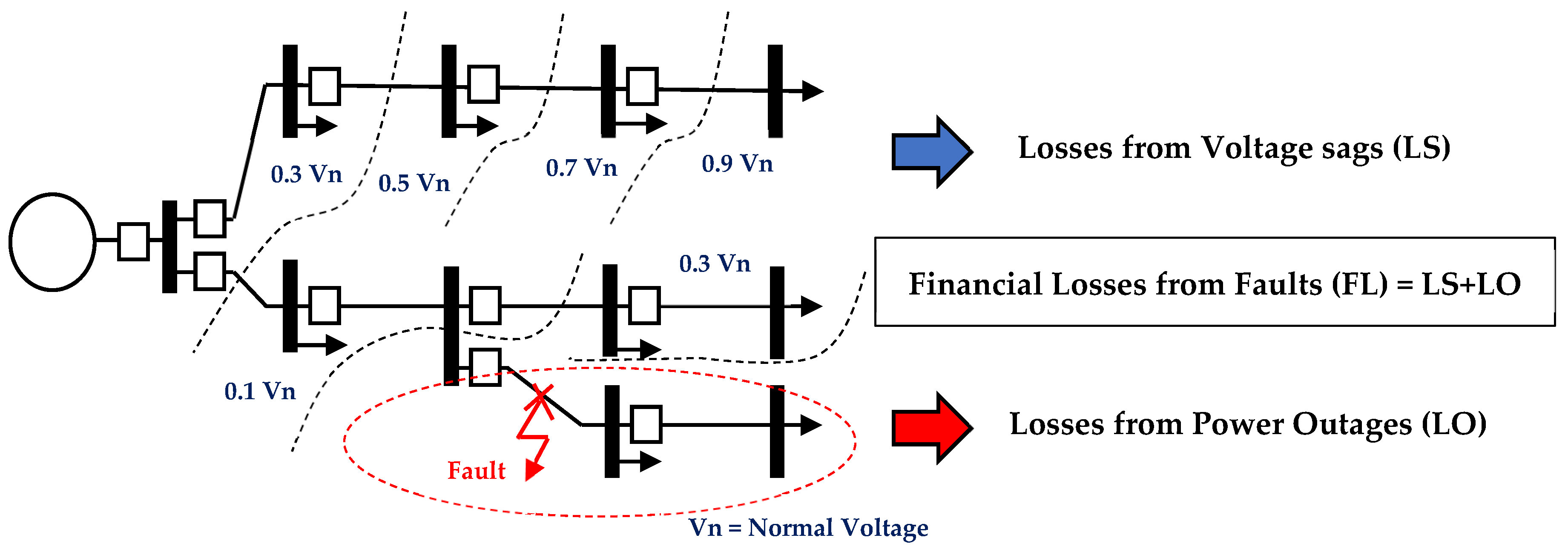
Figure 2.
The fault in the power distribution system.
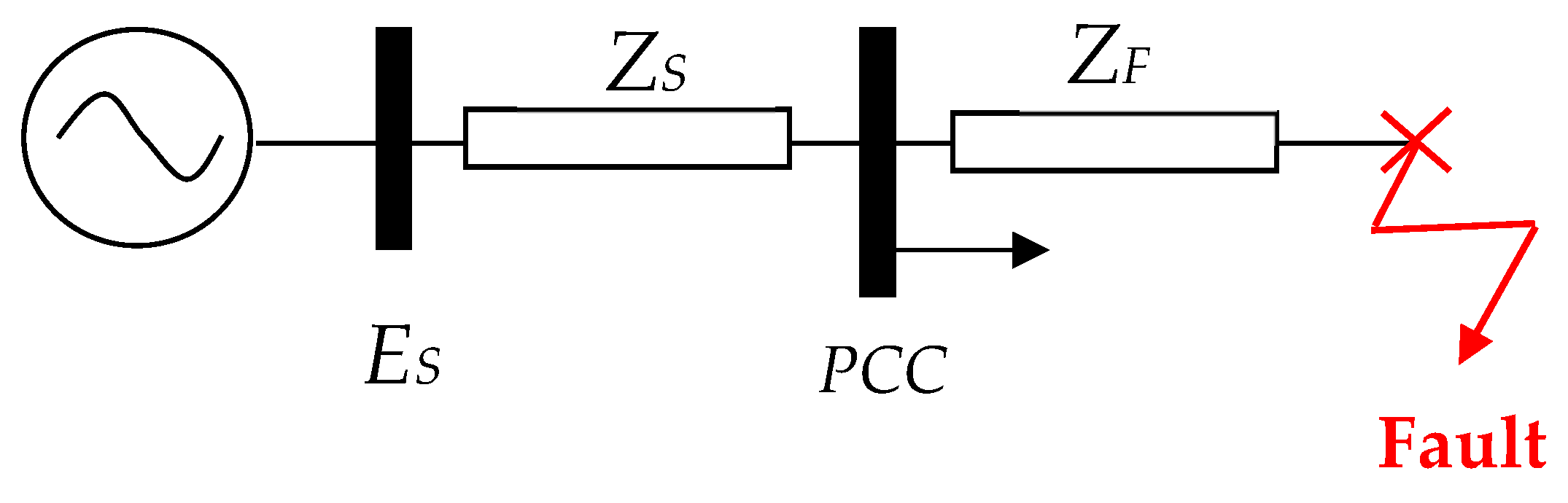
Figure 3.
Saraburi 1 Substation, Provincial Electricity Authority.
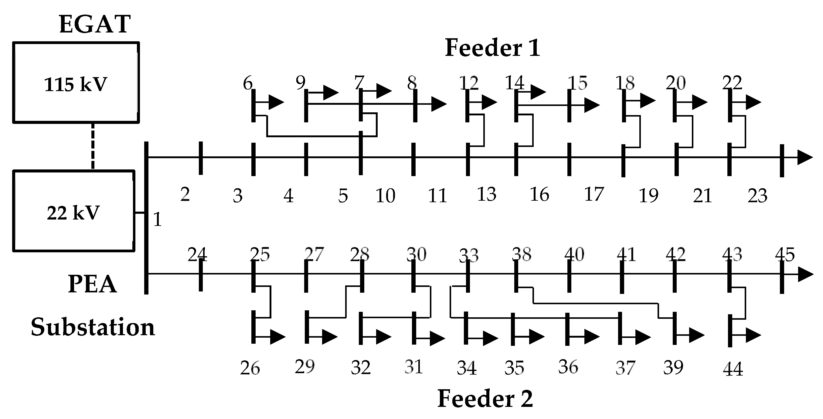
Figure 4.
A diagram for estimating the financial losses caused by faults in the distribution system.
Figure 4.
A diagram for estimating the financial losses caused by faults in the distribution system.
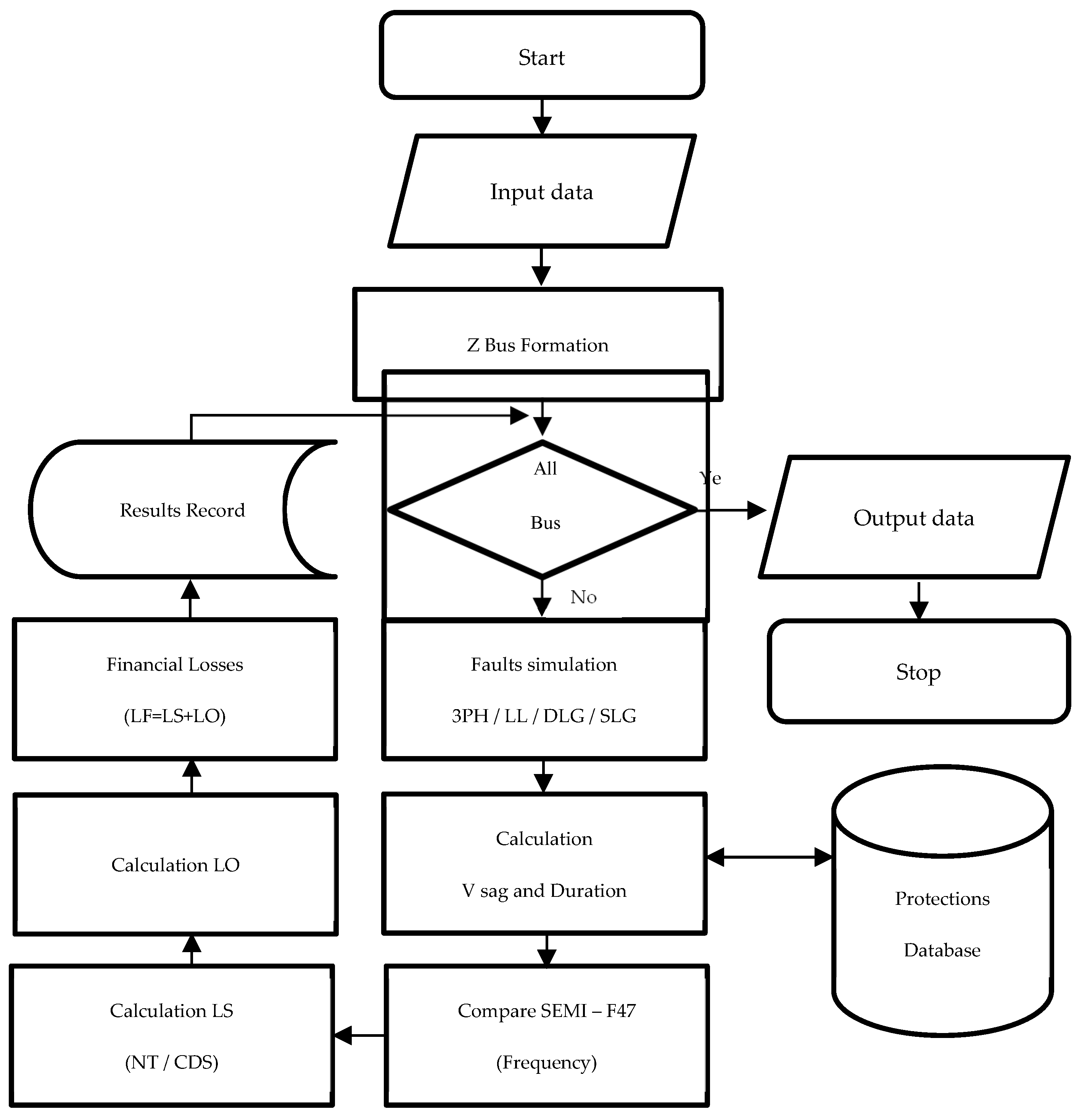
Figure 5.
Comparison of the payback period method, the discounted payback period method, and the net present value method.
Figure 5.
Comparison of the payback period method, the discounted payback period method, and the net present value method.
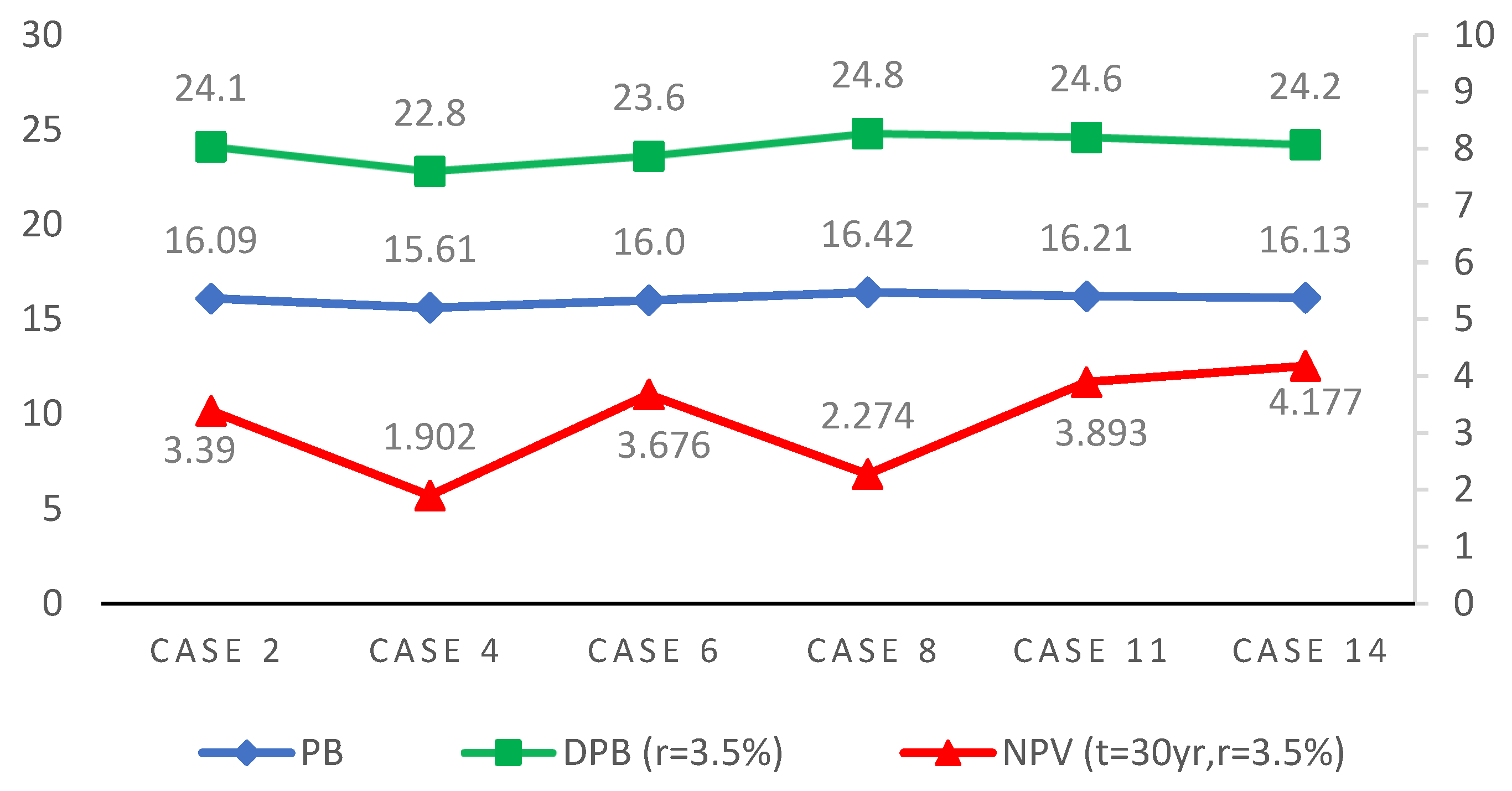
Figure 6.
Compares the cost of improving the power distribution system, the reduced damage, and the ratio of reduced damage per the cost of improving from the top 5 case studies of each method.
Figure 6.
Compares the cost of improving the power distribution system, the reduced damage, and the ratio of reduced damage per the cost of improving from the top 5 case studies of each method.
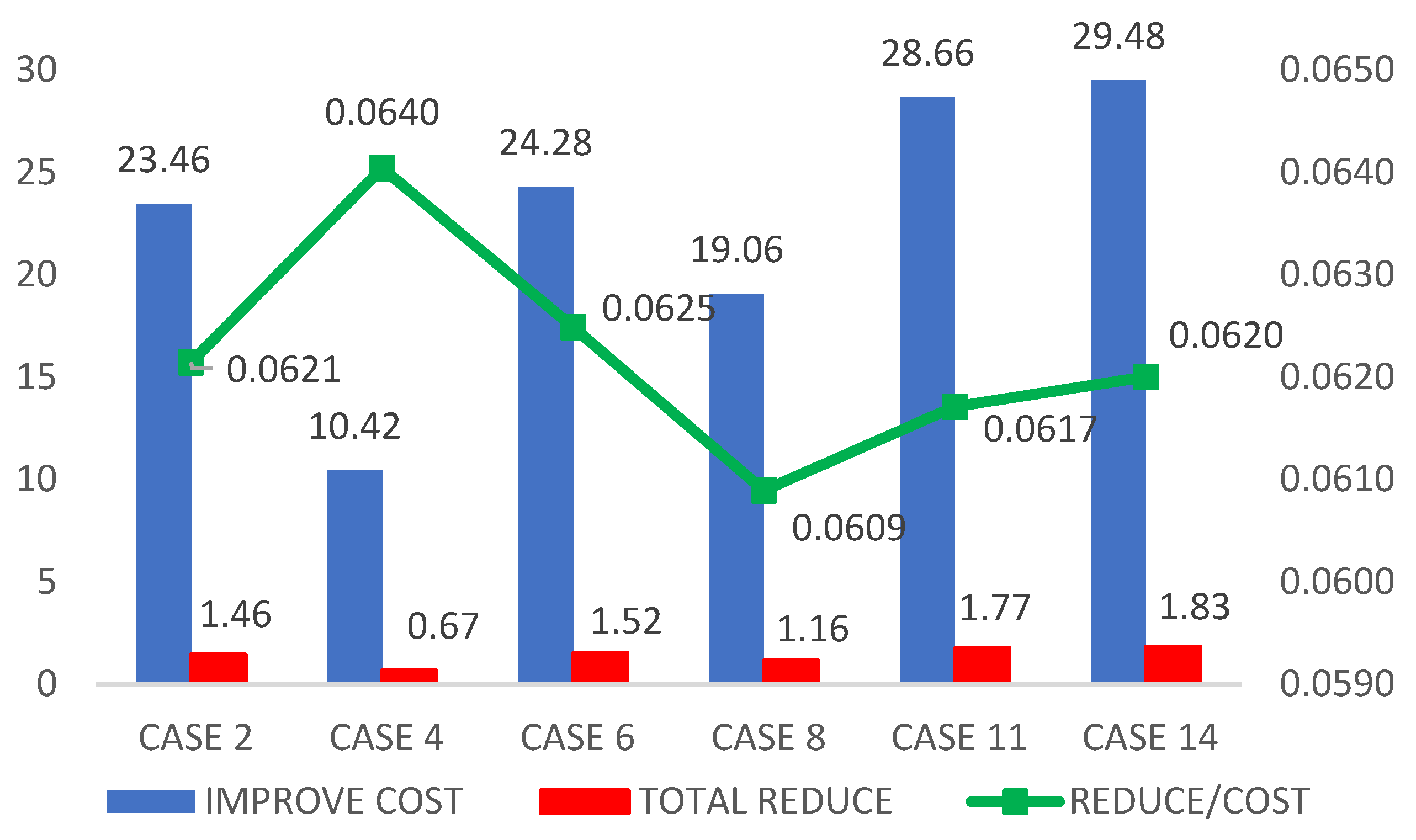
Figure 7.
Route diagram of the power distribution system improvement model.

Table 1.
Conductor information and types of protection devices.
| Bus to Bus |
Distance (km) | Conductor type | Protection type | Bus to Bus |
Distance (km) | Conductor type | Protection type |
|---|---|---|---|---|---|---|---|
| 1-2 | 0.12 | 185 PIC | Relay | 1-24 | 0.15 | 185 SAC | Relay |
| 2-3 | 0.12 | 185 PIC | Relay | 24-25 | 0.15 | 185 SAC | Relay |
| 3-4 | 2.00 | 185 SAC | Relay | 25-26 | 0.30 | 185 PIC | Relay |
| 4-5 | 5.00 | 185 PIC | Relay | 25-27 | 1.50 | 185 PIC | Relay |
| 5-6 | 2.60 | 185 PIC | Relay | 27-28 | 0.10 | 185 PIC | Relay |
| 5-7 | 0.50 | 185 SAC | Relay | 28-29 | 0.20 | 185 SAC | Relay |
| 5-10 | 0.10 | 185 SAC | Relay | 28-30 | 0.65 | 185 SAC | Relay |
| 7-8 | 4.15 | 185 SAC | Relay | 30-31 | 0.75 | 185 SAC | Relay |
| 7-9 | 0.90 | 120 PIC | Relay | 30-33 | 1.15 | 185 SAC | Relay |
| 10-11 | 0.10 | 185 SAC | Relay | 31-32 | 1.50 | 185 PIC | Relay |
| 11-12 | 0.50 | 120 AAC | Relay | 33-34 | 0.50 | 185 PIC | Relay |
| 11-13 | 1.20 | 185 SAC | Relay | 33-38 | 0.50 | 185 PIC | Relay |
| 13-14 | 0.70 | 185 SAC | Relay | 34-35 | 0.20 | 120 AAC | Relay |
| 13-16 | 0.20 | 120 AAC | Relay | 35-36 | 0.80 | 120 AAC | Relay |
| 14-15 | 0.50 | 120 PIC | Fuse | 36-37 | 0.10 | 120 AAC | Relay |
| 16-17 | 0.30 | 120 AAC | Fuse | 38-39 | 0.20 | 185 PIC | Relay |
| 17-18 | 0.10 | 120 AAC | Fuse | 38-40 | 0.50 | 185 PIC | Relay |
| 17-19 | 0.20 | 120 AAC | Fuse | 40-41 | 0.10 | 185 SAC | Relay |
| 19-20 | 1.10 | 120 AAC | Fuse | 41-42 | 0.20 | 185 PIC | Relay |
| 19-21 | 0.30 | 120 AAC | Fuse | 42-43 | 1.00 | 185 PIC | Fuse |
| 21-22 | 1.00 | 120 AAC | Fuse | 43-44 | 0.50 | 120 AAC | Fuse |
| 21-23 | 1.50 | 120 AAC | Fuse | 43-45 | 2.50 | 120 AAC | Fuse |
Table 2.
Resistance and reactance values of conductor.
| Conductor type | R1 (ohm / km) |
X1 (ohm / km) |
R0 (ohm / km) |
X0 (ohm / km) |
|---|---|---|---|---|
| Z th* | 0.06060 | 0.29896 | 0.0000103 | 0.46514 |
| 185 SAC | 0.18050 | 0.24550 | 0.3285000 | 1.75490 |
| 185 PIC | 0.21435 | 0.33976 | 0.3918600 | 1.55380 |
| 120 PIC | 0.26643 | 0.34869 | 0.4144300 | 1.57551 |
| 120 AAC | 0.26643 | 0.36382 | 0.5624300 | 2.70319 |
* Thevenin equivalent impedance of Saraburi 1 Substation (22kV).
Table 4.
Information and costs for improving the power distribution system.
| Improvement pattern | Fault occurrence rate (times/km/year) | Cost of improvement (Million Baht)/km |
|
|---|---|---|---|
| Before improvement | After improvement | ||
| A | 0.250 | 0.225 | 0.20 |
| B | 0.250 | 0.200 | 1.00 |
| C | 0.200 | 0.150 | 1.50 |
Table 5.
Case study of improving the power distribution system.
| Case study | Feeder 1 | Feeder 2 |
|---|---|---|
| 1 | Base case or before improvement. | |
| 2 | Pattern C | Pattern C |
| 3 | Pattern A and C | - |
| 4 | - | Pattern A and C |
| 5 | Pattern A and C | Pattern A and C |
| 6 | Pattern C | Pattern A and C |
| 7 | Pattern A and C | Pattern C |
| 8 | Pattern B and C | - |
| 9 | - | Pattern B and C |
| 10 | Pattern C | Pattern B and C |
| 11 | Pattern B and C | Pattern C |
| 12 | Pattern B and C | Pattern B and C |
| 13 | Pattern A and C | Pattern B and C |
| 14 | Pattern B and C | Pattern A and C |
Table 6.
The result of analysis of losses from voltage sags.
| Case study | Damage costs by type of electricity user (Million Baht) | (A+B+C) Damage cost/year (Million Baht) |
(1) Damage reduction / year (Million Baht) |
||
| A Large load |
B Industrial load |
C Commercial load |
|||
| 1 | 9.42 | 0.94 | 0.24 | 10.59 | - |
| 2 | 8.18 | 0.82 | 0.20 | 9.20 | 1.39 |
| 3 | 8.73 | 0.87 | 0.22 | 9.81 | 0.78 |
| 4 | 8.85 | 0.88 | 0.22 | 9.96 | 0.64 |
| 5 | 8.17 | 0.82 | 0.20 | 9.19 | 1.40 |
| 6 | 8.13 | 0.81 | 0.20 | 9.15 | 1.45 |
| 7 | 8.21 | 0.82 | 0.21 | 9.23 | 1.36 |
| 8 | 8.44 | 0.84 | 0.21 | 9.49 | 1.10 |
| 9 | 8.84 | 0.88 | 0.22 | 9.94 | 0.65 |
| 10 | 8.11 | 0.81 | 0.20 | 9.13 | 1.47 |
| 11 | 7.92 | 0.79 | 0.20 | 8.91 | 1.69 |
| 12 | 7.86 | 0.79 | 0.20 | 8.84 | 1.76 |
| 13 | 8.05 | 0.80 | 0.20 | 9.06 | 1.53 |
| 14 | 7.87 | 0.79 | 0.20 | 8.85 | 1.74 |
Table 7.
The result of analysis of losses from power outages.
| Case study | D Opportunity cost of selling electricity (Million Baht) |
E Cost of fixing power outages (Million Baht) |
(D+E) Damage Cost/Year (Million Baht) |
(2) Damage reduction / year (Million Baht) |
|---|---|---|---|---|
| 1 | 0.192 | 0.361 | 0.553 | - |
| 2 | 0.164 | 0.322 | 0.486 | 0.0669 |
| 3 | 0.171 | 0.331 | 0.502 | 0.0503 |
| 4 | 0.183 | 0.340 | 0.523 | 0.0296 |
| 5 | 0.162 | 0.310 | 0.473 | 0.0799 |
| 6 | 0.164 | 0.317 | 0.481 | 0.0721 |
| 7 | 0.162 | 0.316 | 0.478 | 0.0747 |
| 8 | 0.170 | 0.325 | 0.495 | 0.0581 |
| 9 | 0.183 | 0.335 | 0.518 | 0.0349 |
| 10 | 0.164 | 0.312 | 0.475 | 0.0773 |
| 11 | 0.161 | 0.309 | 0.470 | 0.0825 |
| 12 | 0.161 | 0.299 | 0.460 | 0.0929 |
| 13 | 0.162 | 0.305 | 0.468 | 0.0851 |
| 14 | 0.161 | 0.304 | 0.465 | 0.0877 |
Disclaimer/Publisher’s Note: The statements, opinions and data contained in all publications are solely those of the individual author(s) and contributor(s) and not of MDPI and/or the editor(s). MDPI and/or the editor(s) disclaim responsibility for any injury to people or property resulting from any ideas, methods, instructions or products referred to in the content. |
© 2024 by the authors. Licensee MDPI, Basel, Switzerland. This article is an open access article distributed under the terms and conditions of the Creative Commons Attribution (CC BY) license (http://creativecommons.org/licenses/by/4.0/).
Copyright: This open access article is published under a Creative Commons CC BY 4.0 license, which permit the free download, distribution, and reuse, provided that the author and preprint are cited in any reuse.


