
Submitted:
18 December 2024
Posted:
19 December 2024
You are already at the latest version
Abstract
To improve the observation efficiency of the space debris survey, a basic sky survey observation strategy has been developed, aiming to observe more space debris based on the Wide Field Optical Telescope Array running by Shandong University. The characteristics of the telescope and dynamic changes in the movement position of space debris are considered in this strategy. An objective function is designed based on these factors. By using the pixelated sphere method to finely divide the celestial area, applying the summation filtering method, and using the greedy algorithm, the benefit of the objective function can be maximized, thus generating the optimal sky survey observation strategy. We demonstrated, through simulation and observation experiments , that the observation strategy using the greedy algorithm significantly improved the number of space debris and the number of arc segments with respect to the conventional observation strategy. This not only improves the automation level of the space debris observation plan but also significantly enhances the execution efficiency of the telescopes for debris observation. It is very helpful for cataloging space debris and collision warnings.
Keywords:
Observation Strategy
; Pixelized Sphere
; Objective Function
; Greedy Algorithm
1. Introduction
In recent decades, the sky survey has become an important observation approach[1,2,3,4,5]. In sky survey projects, scientists would use a telescope to collect images according to predefined strategies. Scientists would use these images to study large scale structure of the Universe or discover new transients. Nowadays,celestial objects with fast variations have attracted many attentions and have become main targets studied by the time domain astronomy. Because some fast variations in temporal domain are caused by astrophysical phenomenons in very small space scale, some celestial objects with fast variations are either astronomical phenomenons with very high energy(such as mergers of compact stars, super-flares or TDEs) or astronomical targets that are very close to us (such as NEOs or artificial space debris).
The Zwicky Transient Facility (ZTF)[6] focuses on detecting time-domain astronomical events such as supernovae, tidal disruption events (TDEs), active galactic nuclei (AGNs), and electromagnetic counterparts to gravitational wave events. The ZTF scheduler determines which fields to observe and in what order. Integer Linear Programming techniques inspired by Lampoudi et al.[7] maximize the volumetric survey speed using slot-based lookahead throughout the night. All ZTF images are obtained on a fixed grid of fields with minimal dithering. The primary grid covers the entire sky with an average overlap between fields of about 0.26° in Decl. and about 0.29° in R.A. The fields are aligned to cover the Galactic Plane region with the fewest pointings, improving the efficiency of both Galactic and extragalactic surveys.
The Vera C. Rubin Observatory’s Legacy Survey of Space and Time (LSST)[8] aims to map a survey area of 20,000 square degrees in the southern hemisphere, with 180 visits over a 10-year period, achieving a detection limit of r=28.0 magnitudes. The observation strategy will be carefully reviewed based on metrics designed by different scientific working groups, including the Science Requirements Document (SRD) metrics and the Dark Energy Science Collaboration (DESC) Wide-Fast-Deep (WFD) metrics, which incorporate supernovae, TDEs, fast microlensing events and so on. Naghib et al.[9] used a Markov decision process to solve the tour scheduling problem at the Villa C. Rubin Observatory by constructing a feature-based telescope scheduler within a coherent mathematical model.
The Wide Field Survey Telescope (WFST) [10] is located in Qinghai Province, China. Its primary scientific goals include the study of extragalactic transient phenomena such as supernovae, tidal disruption events (TDEs), and active galactic nuclei (AGN). Other vital programs include near-Earth objects (NEOs), Galactic satellites, galaxy formation, and cosmological studies. Taking various factors into account, a primary sky survey strategy was designed to maximize the capabilities of the instruments and ensure the best possible results. The sky area is divided into rectangular regions, called “tiles”, with a size of 2.577° × 2.634°, slightly smaller than the focal area of a mosaic CCD. A dedicated dithering pattern is proposed to cover the gap between the CCDs and the four corners of the mosaic CCD array, which lie outside the 3° field of view. This dithering pattern helps to achieve a relatively uniform exposure map for the final survey output.
Neural network-based optimization algorithms have been employed for scheduling observations with the Hubble Space Telescope[11]. The RTS2 (Remote Telescope System 2nd Edition) system is a well-known open-source software for autonomous telescope observations in the field. Initially, it used a simple value function to optimize survey scheduling but was later enhanced to include genetic algorithms[12].
Since telescope arrays have many objects to observe, Jia et al.[13] investigated an optimal control strategy to maximize their scientific output. A framework, which includes a simulator and a reinforcement learning-based algorithm, is proposed to obtain an optimal control strategy for the Wide Field of View Small Aperture Telescope Array based on predefined scientific requirements.
A multilevel scheduling model was proposed for the telescope array scheduling question for time-domain measurements by Zhang et al.[14] A flexible framework was developed with its essential functions encapsulated in software components implemented on a layered architecture. An optimization metric was proposed for self-consistently weighing the contributions from time-varying observation conditions to maintain uniform coverage and efficient time utilization from a global perspective. The performance of the scheduler is evaluated through simulation examples.
In recent years, machine learning-based policy optimization algorithms have been widely discussed[15,16,17,18,19]. In order to reduce the computational cost and complexity of these algorithms, there are many assumptions that deviate from the actual observing conditions. There are millions of celestial objects to be observed every night. At the same time, we have limited telescopes, and the observing ability of these telescopes can be affected by different factors, such as sky background or observing conditions. Jia et al.[20] proposed a novel framework that included a digital simulation environment and a deep reinforcement learning algorithm for optimizing the observation strategy of a telescope array. The framework can obtain effective observing strategies based on predefined requirements and observing environment information.
In the face of the current severe environment of space debris, ground-based optical monitoring with multiple means, full scale, and all-sky area is a significant trend for future development. The high degree of flexibility of ground-based optical monitoring places higher demands on developing observation strategies, which is also an important factor affecting its observational effectiveness.
Previous investigations about observation strategy, mostly describing the survey observation of astronomical targets, rarely dealt with the survey observation strategy of space debris. The observation strategy of space debris is more complicated, the orbits of individual debris are different, and they are fast-moving and dynamically changing. In order to improve efficiency, when we utilize ground-based optical telescopes for space debris observation, we need to formulate different observation strategies according to different mission requirements, debris information, equipment conditions, and other factors. At the same time, when there are multiple debris to be observed, it is necessary to solve the multi-objective optimization problem, construct the objective function, and select and sort the candidate debris. A suitable observation strategy can not only improve the data quality but also improve the execution efficiency of the telescope and maximize the benefit.
In this work, with the task requirement of observing more space debris, we propose a survey observation strategy based on the greedy algorithm and HEALPix algorithm. The optimal observation strategy is derived by pre-setting the telescope parameters and combining the summation filter, pixelated sphere algorithm, and greedy algorithm based on the debris forecast information. In order to test the performance of the observation strategy, we conducted experiments with the Wide Field Optical Telescope Array (hereafter: WFOTA) running by Shandong University. The results show that our observation strategy can observe more space debris and performs better than the ordinary method. We discuss the design of the objective function in Section 2, the design of the spherical pixelization method using HEALPix and summation filter, and the application of the greedy algorithm to the objective function. In Section 3, we demonstrate the performance of the observation strategy using simulation and observation experiments. We conclude and predict our future work in Section 4.
2. Methods
2.1. Objective Function
The requirements of the objective function are different for different observation tasks and research objectives. In this work, our task is to obtain as more space debris observations as possible during a given period using the given telescopes. We need to divide the whole celestial sphere into several small celestial regions, and the size of the divided celestial regions is the size of the celestial regions observed by the telescope, i.e., the size of the telescope’s field of view. By using an observing strategy that minimizes the time required for each rotation of the telescope and maximizes the amount of space debris in each observed sky region (i.e., at each time step), we need to form an observing plan for each night. An observing schedule for each night is formed so that, ultimately, more space debris can be observed each night, with the following objective function:
where denotes the set of sky regions for each observation from 1 to T each night, denotes the spherical angular distance of the two successive neighboring regions, and denotes the set of sky regions with the largest number of space debris.
Because space debris is in rapid motion at all times, in order to obtain the observation sky area for more space debris mentioned in the objective function, it is necessary to know the orbital information of each space debris at each moment of the night for orbital forecasting.
2.2. Orbital Forecasting of Space Debris and Optimization of Orbital Information
The latest TLE data are obtained, and the orbital information of the debris on the day is obtained through orbital computation. The main objective of the orbit calculation is to determine the real-time position and visibility parameters of the debris. This includes the time of darkness at the station, the time of debris visibility, the time of visibility of the debris at the station during darkness, and the time that the debris is illuminated by the sun during the time of visibility, obtaining data information such as the declination, latitude, altitude angle, azimuth, and the debris number of the different debris at each moment.
The parameters are set according to the observatory site, telescope situation, and observing needs, and the observation lasts for a fixed period of time in each observing sky area, which is called the time step. In order to ensure that all the fragments within the time step are valid and to prevent the situation of running out of the field of view just after entering the field of view, and at the same time, we need at least five images in the data processing in order to recognize the space debris, the frequency of the same debris appearing within the time step will be processed, and the processing criterion will be met when the number of times of its appearance is greater than or equal to 5 (in order to prepare for the subsequent detection of the space debris). The same debris within the specified time step will be counted only once, thus ensuring the maximum number of unrepeated fragments. The same debris within a specified time step is counted only once, thus ensuring the maximum number of single non-repeating debris.
After we get the orbit information in a fixed time step, we need to divide the sky area. In this work, we apply Spherical Pixelization Method using HEALPix to discretize the spherical data. HEALPix is an advanced method for discretization and fast analysis of high-resolution spherical data, and its main features include equal-area pixelization and hierarchical structure, which makes the data more uniformly distributed in the spherical surface, effectively avoiding the distortion problem common to other pixelization methods [21].
2.3. Spherical Pixelization Method Using HEALPix
HEALPix divides the sphere into 12 base pixels, which can be recursively subdivided in subsequent layers in multiples of 4 to form a hierarchical equal-area pixel structure, which helps in the unbiased statistical analysis of the data[22], as shown in Figure 1.
The resolution of HEALPix is defined by the parameter. The higher the value, the higher the number of pixels and the higher the resolution. We choose the appropriate , which means that the sphere is divided into equal area pixels. The choice of weighs computational efficiency and space resolution, ensuring data accuracy while maintaining computational manageability1.
We map space debris data points to the HEALPix grid using their spherical coordinates (Right Ascension and Declination). Each data point is assigned to a corresponding pixel within a pixel, and the coordinates are converted to pixel indices using the function in the HEALPix library. Once the data are pixelated, statistical calculations such as averaging and summing can be performed directly on the pixelated data. This approach simplifies data processing and increases computational speed 2. We used the HEALPix software package (available in C++ and Python) for pixelization and data analysis. The Python library was explicitly used due to its easy integration with other data processing tools and ease of use.
In this work, the Spherical Pixelization Method is used to divide the celestial region of the whole celestial sphere. From the definition of resolution in HEALPix, the parameter is taken to be 32, and the celestial sphere is divided into 12,288 equal-area pixels. The function in the HEALPix library is used to convert the celestial sphere equatorial coordinates to pixel indexes. The function in HEALPix is used to convert the pixel indexes to the spherical coordinates of the pixel centers. The function is used to compute the spherical coordinates of the four boundaries of each pixel, which forms a pixel region. Within the time step, the count is increased by one if the space debris’s declination is within the pixel area. The debris density of the specified pixel region within the current time step is derived by the following Equation 3, as shown in Figure 2 as the heat map distribution of the space debris density distribution within the non-empty pixels at any time step in the equatorial coordinate system (time step of 2 minutes).
In the formula, represents the number of debris in the kth pixel during the ith time step, and S represents the area of the pixel.
We obtain the distribution of space debris at each pixel on the celestial sphere, and in order to relate it to the telescope field of view, we apply the summation filter method, which skillfully combines the telescope field of view with specific pixels on the celestial sphere to obtain the observation sky area.
2.4. Additive Sum Filtering and the Greedy Algorithm
We set the size of the filter according to the field of view of the telescope, with 2° and 1° overlap in the declination and right ascension directions, respectively, in order to prevent debris from being missed. We regard the telescope field of view as a filter, which is the size of the effective observation field of view. WFOTA is used in this work as an example, and the effective field of view is 9° × 18°. The center of the filter is taken to be the center coordinate of the pixel, and the filter range covers all areas around the pixel whose coordinates satisfy the field of view constraints. A surrounding pixel whose spherical angular distance from the center coordinate is less than half of the field of view is considered to be inside the filter, and the boundary conditions of the filter are shown in Equation 4. A filter centered on each pixel yields a list of data that traverses each non-empty pixel to obtain the distribution of fragments within the different filters (including the filter’s declination coordinates, the number of fragments, and the ). The distribution of fragments in the field of view is obtained using this additive and filtering approach. The boundary conditions of the filter are:
The total number of fragments contained within the filter constructed with pixel j at the ith time step is defined as . For each time step i, we construct the filter for all pixels j and record the following information: the coordinates of the filter center ; the total number of fragments within the filter ; and the unique set of fragments within the filter.
where denotes the fragmentation density distribution of pixel k in time step i. is the set of pixels centered at pixel j that cover the filter range. By traversing all pixels j, the distribution of fragments within the filter at its center can be calculated and the concentration of fragments in it can be evaluated.
After we did the summing filter, we got the distribution of space debris within each filter within each time step. The next step to do is to pick the filter with the most fragments from each time step. However, there will be a situation where there may be more than one filter with the same maximum number of fragments in each time step, forming the set of maximal number of fragments filters.
In order to optimize the observation strategy, the most suitable observation is selected from these, which we measure based on the magnitude of the spherical angular distance between the 2-time steps before and after. We used a greedy algorithm to schedule the observations for each night. That is, the field of view points to the sky area where the most significant number of filters is located in the current time step. The telescope pointing for the next step is the sky area closest to the current pointing, and the largest filter is located in that time step. The optimization algorithm has the advantages of simplicity, efficiency, and ease of implementation. The basic idea is to take the best choice in the current state at each selection step so that the final result is optimal. The scheduling optimization can be decomposed into subproblems, precisely the optimization problem for each night or each observation. Before each observation, the sky zone pointing that costs the least to move the telescope and has the highest payoff metric is chosen to obtain a locally optimal solution. Once the optimal observations are collected, the entire scheduling can be optimized.
We pick the unique maximum number of fragments filter within each time step by time step. The process is described below:
(1) Initial time step
Calculate the number of fragments for all filters: for an initial time step , calculate the total number of fragments for each filter to get the maximal fragmentation value . Select the set of filters with the maximum number of fragments:
If there is only one filter in the set of maximum filters: select that filter directly, denoted .If there is more than one filter in the set of maximum filters: choose the one closest to the observatory as .Record as the initial filter and remove its observed fragments from the fragmentation library, i.e., the fragmentation counts in subsequent filters do not contain space debris within the recorded filters.
(2) Subsequent time step
Update debris repository: At the beginning of each time step, remove from the repository all debris that has been observed from the debris repository (including debris observed in in previous steps). The debris library is updated to: .
Calculate the number of fragments in the current time step: In time step i, the number of fragments for each filter in the remaining fragmentation bank is calculated. Further, we obtain the filter with the maximum number of fragments . Find the corresponding set of filters with maximum number of fragments:
(3) Apply the greedy algorithm to select the most suitable filter
Select the unique filter with the closest distance to the spherical angle and the maximum number of fragments. If there are multiple filters in the set , calculate their spherical distances from the selected filter from the previous time-step and select the filter with the smallest distance filter with the smallest distance.
where, : denotes the distance between the center of the filter j and the center of on the sphere.Record the result: remove the observation fragments of the selected filter from the fragment bank.
(4) Loop to end of time step
For each time step, the above steps are repeated: the number of fragments for each filter in the remaining fragment bank is calculated, the filter with the highest number of fragments is found, if there are multiple filters with the maximum number of fragments, a greedy algorithm is applied to select the closest filter, and the observed fragments of the selected filter are removed, and the fragment bank is updated. And so on until the end of the last time step.
We uniquely assign fragments, and filter selection at each time step is based on a real-time updated fragment bank. We use a greedy algorithm to optimize the time continuity. We prefer the filter with the closest distance to the previous time step when the number of fragments is the same to improve the observation continuity and efficiency. Only one unique filter is selected in each time step, suitable for gradually planning the observation task. The final output is a list of unique maximum fragment number filters , in Equation 1 .
3. Experiments and Results
3.1. Instrument Parameters
In order to test the performance of the observation strategy, we conducted experiments with the Wide Field Optical Telescope Array (hereafter: WFOTA) running by Shandong University, China. WFOTA consists of four 15-centimeter aperture optical telescopes with large fields of view (FOVs), with a single telescope having a field of view of about 100 square degrees and a total field of view of up to 400 square degrees. The four telescopes are mounted in groups of two on two turntables, and the two telescopes on one turntable have a stitched field of view of 10° x 18°.
3.2. Experiment
In order to verify the validity of the methods, simulation experiments were done, and additionally observation experiments were done at the same time to compare the results of the various methods.
We obtained TLE data for all space debris on September 2 and September 3, 2024, from the Space-track website. Based on the environmental conditions of WFOTA, the altitude angle limit is set to be greater than 20°, the surrounding buildings and mountains occlude the azimuth angle between 12° and 20°, so this angle range is skipped. The sampling interval of the data points was taken as 2 seconds, and the orbit prediction calculation was performed to obtain the visible time, right ascension, declination, altitude angle, and azimuth of the debris.
According to the requirements of the actual observation, we adopt a two-minute time step, which means that the pointing in each sky region is continuously imaged for two minutes, with exposures every 2 seconds, and the data readout time is about 0.98 seconds. By applying the methods of orbit forecast data optimization and pixelated spheres, the space debris density distributions for all time steps on September 2 and September 3 were obtained, respectively, and an example is shown in Figure 3 ( the first six time steps on September 2)
For comparison, we used two sets of telescopes each night to ensure that the observation conditions were the same at the time of the observations: on the night of September 2, one set of telescopes with the observation strategy using the greedy algorithm and one set of telescopes with the randomized observation strategy, and on the night of September 3, one set of telescopes with the greedy algorithm and one set of telescopes with the all-sky coverage observation strategy, We compared the results with two separate sets of telescopes.
3.2.1. Randomized Observation Strategy
Based on the results of the orbit calculations and the data processing results of the pixelated spherical method, one filter is randomly selected within each time step as the telescope pointing to obtain the telescope observation field of view for the whole night of September 2. An example is shown in Figure 4 (the first 6), and the final WFOTA field of view pointing to the celestial sphere is shown in Figure 5.
3.2.2. Observation Strategy for Greedy Algorithm
We optimize the time continuum by means of a greedy algorithm. We select only one filter as the unique optimal telescope pointing within each time step. It is guaranteed that the telescope requires the least amount of time for each rotation and that the amount of space debris in the sky region observed is maximized each time. The telescope observation fields of view for two full nights on September 2 and September 3, 2024 are obtained. An example is shown in Figure 6 (the first 6), and the WFOTA field of view that finally points to the celestial sphere is shown in Figure 7.From the figure we can see that pointing is clearly different from random pointing.
3.2.3. Observation Strategy for All-Sky Coverage
According to the results of orbit calculation and pixelated sphere data processing, all telescope observation fields of view for each time step are obtained for the whole night of September 3, 2024. Using the all-sky coverage observation strategy, we take one active field of view in each time step in the order of the time steps. Moreover, each observation field of view does not overlap and eventually covers all the observable sky area, get all the effective observation fields of view, as an example, as shown in Figure 8 to take (the first six steps as a schematic), the final WFOTA field of view in the celestial sphere pointing as shown in Figure 9.
3.3. Result
Table 1 shows the results of the simulation and observation experiments on September 2, 2024 using the observation strategy of the greedy algorithm and the observation strategy of random observation. Table 2 shows the results of the simulation and observation experiments on September 3, 2024, using the observation strategy of the greedy algorithm and the observation strategy with all-sky coverage. We compare the number of space debris and the number of arc segments of space debris.
From the simulation results, we can see that in the comparison of the number of space debris, the observation strategy using the greedy algorithm improves by 104.6% compared to the random observation strategy. The observation strategy using the greedy algorithm improves by 250.2% compared to the observation strategy with all-sky coverage. At the same time, we also compare the number of space debris arcs, which is 26.8% higher in the greedy algorithm than in the randomized observation strategy. The observation strategy using the greedy algorithm has an improvement of 263.3% compared to the observation strategy with all-day coverage.
According to the observation strategy of the simulation, the observation plan is derived, and the observation is executed with WFOTA to obtain the observation data. The target detection method involved through data processing, we utilize the 3D Hough transform to detect moving objects in photometric images[23]. In terms of the comparison of the number of space debris, the observation strategy using the greedy algorithm improves 89.1% in comparison with the random observation strategy. The observation strategy using the greedy algorithm improves by 268.1% compared to the observation strategy with all-sky coverage. Regarding the comparison of the number of space debris arc segments, the observation strategy using the greedy algorithm improves by 29.2% compared to the random observation strategy, and the observation strategy using the greedy algorithm improves by 257.7% compared to the observation strategy with all-sky coverage.
By using the pixelated sphere method, the summation filtering method, and the greedy algorithm, the observation strategy is greatly improved compared with the traditional observation strategy, no matter the number of space debris or the number of arc segments in the simulation or the actual measurement. Moreover, the greedy algorithm is more purposeful and will not miss the space debris gathering area, which makes the observation more reasonable. It can significantly improve the speed of the telescope debris observation plan and optimize the degree of automation of the debris observation plan.
4. Discussion
Developing an observation strategy for space debris is a highly complex task, and the survey observation strategy proposed In this work can simplify the process of developing a space debris observation plan and significantly improve the execution efficiency of space debris observation. Our primary research results are summarized as follows:
1. Our task is to obtain as more space debris observations as possible during a given period using the given telescopes.We establish an objective function with full consideration of debris information, equipment conditions and other factors. The space debris is dynamically changing. The application of the pixelized sphere HEALPix algorithm and the method of summation filtering to calculate the distribution of debris density within each sky region in real-time are very important. The problem of deformation in sky regions located near the poles is effectively avoided, which contributes to the unbiased statistical analysis of the data. The field of view of the telescope is equated to an equal-sized filter, which effectively speeds up the data processing.
2. By using a greedy algorithm, the best choice is made at each time step under the current conditions, the optimal observations are collected, and the whole scheduling process is continuously optimized to ensure the optimal final result. Compared with random observation and all-sky coverage, the greedy algorithm significantly improves the number of space debris and the number of arcs on both simulation and observation experiments .
An increased number of space debris and arc segments is beneficial for cataloging space debris, continuously enriching the catalog, and providing solid data support for cataloging space debris and collision warnings. The survey observation strategy program can be continuously improved as we gain a deeper understanding of observational conditions and facility characteristics. In the future, we plan to research other optimization algorithms and consider more detailed simulations to improve the efficiency of space debris observation further.
Author Contributions
Conceptualization, S.L., S.H. and J.D.; methodology, S.L. and J.D; program, S.L. and J.D.; validation, H.C. and S.H.; formal analysis, S.L.; investigation, S.L.; resources, S.L. and Y.J; data curation, S.L. and Y.J.; writing—original draft preparation, S.L.; writing—review and editing, S.L., S.H., J.D., Y.J and S.F.; visualization, S.L., S.H., J.D., Y.J. and S.F.; supervision, S.H.; project administration, S.H.; funding acquisition, S.H. All authors have read and agreed to the published version of the manuscript.
Funding
This work is supported by the Natural Science Foundation of China under grant No.12373015 and No.12303104.
Data Availability Statement
All synthetic data from the authors are available.
Conflicts of Interest
The authors declare no conflict of interest.
References
- Solar, M.; Michelon, P.; Avarias, J.; Garcés, M. A scheduling model for astronomy. Astronomy and Computing 2016, 15, 90–104. [Google Scholar] [CrossRef]
- Tonry, J.; Denneau, L.; Heinze, A.; Stalder, B.; Smith, K.; Smartt, S.; Stubbs, C.; Weiland, H.; Rest, A. ATLAS: a high-cadence all-sky survey system. Publications of the Astronomical Society of the Pacific 2018, 130, 064505. [Google Scholar] [CrossRef]
- Morris, B.M.; Tollerud, E.; Sipocz, B.; Deil, C.; Douglas, S.T.; Medina, J.B.; Vyhmeister, K.; Smith, T.R.; Littlefair, S.; Price-Whelan, A.M.; others. Astroplan: an open source observation planning package in Python. The Astronomical Journal 2018, 155, 128. [Google Scholar] [CrossRef]
- Shimwell, T.; Hardcastle, M.; Tasse, C.; Best, P.; Röttgering, H.; Williams, W.; Botteon, A.; Drabent, A.; Mechev, A.; Shulevski, A.; others. The LOFAR two-metre sky survey-V. Second data release. Astronomy & astrophysics 2022, 659, A1. [Google Scholar]
- Lacy, M.; Baum, S.; Chandler, C.; Chatterjee, S.; Clarke, T.; Deustua, S.; English, J.; Farnes, J.; Gaensler, B.; Gugliucci, N.; others. The Karl G. Jansky very large array sky survey (VLASS). Science case and survey design. Publications of the Astronomical Society of the Pacific 2020, 132, 035001. [Google Scholar] [CrossRef]
- Bellm, E.C.; Kulkarni, S.R.; Graham, M.J.; Dekany, R.; Smith, R.M.; Riddle, R.; Masci, F.J.; Helou, G.; Prince, T.A.; Adams, S.M.; et al. The Zwicky Transient Facility: System Overview, Performance, and First Results. Publications of the Astronomical Society of the Pacific 2018, 131, 018002. [Google Scholar] [CrossRef]
- Lampoudi, S.; Saunders, E.; Eastman, J. An Integer Linear Programming Solution to the Telescope Network Scheduling Problem. arXiv e-prints, arXiv:1503.07170.
- Željko Ivezić; Kahn, S.M.; Tyson, J.A.; Abel, B.; Acosta, E.; Allsman, R.; Alonso, D.; AlSayyad, Y.; Anderson, S.F.; Andrew, J.; et al. LSST: From Science Drivers to Reference Design and Anticipated Data Products. The Astrophysical Journal 2019, 873, 111.
- Naghib, E.; Yoachim, P.; Vanderbei, R.J.; Connolly, A.J.; Jones, R.L. A Framework for Telescope Schedulers: With Applications to the Large Synoptic Survey Telescope. The Astronomical Journal 2018, 157. [Google Scholar] [CrossRef]
- Wang, T.; Liu, G.; Cai, Z.; Geng, J.; Fang, M.; He, H.; Jiang, J.a.; Jiang, N.; Kong, X.; Li, B.; others. Science with the 2.5-meter wide field survey telescope (wfst). Science China Physics, Mechanics & Astronomy 2023, 66, 109512. [Google Scholar]
- Johnston, M.; Adorf, H.M. Scheduling with neural networks—the case of the hubble space telescope. Computers & Operations Research 1992, 19, 209–240. [Google Scholar]
- Kubanek, P. Genetic algorithm for robotic telescope scheduling. arXiv e-prints, arXiv:1002.0108.
- Jia, Q.; Jia, P.; Liu, J. Optimal control of wide field small aperture telescope arrays with reinforcement learning. Observatory Operations: Strategies, Processes, and Systems IX. SPIE, 2022, Vol. 12186, pp. 205–212.
- Zhang, Y.; Yu, C.; Sun, C.; Shang, Z.; Hu, Y.; Zhi, H.; Yang, J.; Tang, S. A multilevel scheduling framework for distributed time-domain large-area sky survey telescope array. The Astronomical Journal 2023, 165, 77. [Google Scholar] [CrossRef]
- Milani, A.; Farnocchia, D.; Dimare, L.; Rossi, A.; Bernardi, F. Innovative observing strategy and orbit determination for Low Earth Orbit space debris. Planetary and Space Science 2012, 62, 10–22. [Google Scholar] [CrossRef]
- Ferreira, J.; Hussein, I.; Gerber, J.; Sivilli, R. Optimal SSN tasking to enhance real-time space situational awareness. Proceedings of the AMOS Technical Conference, 2016, pp. 20–23.
- Hinze, A.; Fiedler, H.; Schildknecht, T. Optimal scheduling for geosynchronous space object follow-up observations using a genetic algorithm. Advanced Maui Optical and Space Surveillance Technologies Conference (AMOS). Maui Economic Development Board Maui, HW, 2016.
- Frueh, C.; Fielder, H.; Herzog, J. Heuristic and optimized sensor tasking observation strategies with exemplification for geosynchronous objects. Journal of Guidance, Control, and Dynamics 2018, 41, 1036–1048. [Google Scholar] [CrossRef]
- Cai, H.; Yang, Y.; Gehly, S.; He, C.; Jah, M. Sensor tasking for search and catalog maintenance of geosynchronous space objects. Acta Astronautica 2020, 175, 234–248. [Google Scholar] [CrossRef]
- Jia, P.; Jia, Q.; Jiang, T.; Liu, J. Observation strategy optimization for distributed telescope arrays with deep reinforcement learning. The Astronomical Journal 2023, 165, 233. [Google Scholar] [CrossRef]
- Gorski, K.M.; Hivon, E.; Banday, A.J.; Wandelt, B.D.; Hansen, F.K.; Reinecke, M.; Bartelmann, M. HEALPix: A framework for high-resolution discretization and fast analysis of data distributed on the sphere. The Astrophysical Journal 2005, 622, 759. [Google Scholar] [CrossRef]
- Zonca, A.; Singer, L.; Lenz, D.; Reinecke, M.; Rosset, C.; Hivon, E.; Gorski, K. healpy: equal area pixelization and spherical harmonics transforms for data on the sphere in Python. Journal of Open Source Software 2019, 4, 1298. [Google Scholar] [CrossRef]
- Zhang, B.; Hu, S.; Du, J.; Yang, X.; Chen, X.; Jiang, H.; Cao, H.; Feng, S. Detecting Moving Objects in Photometric Images Using 3D Hough Transform. PUBLICATIONS OF THE ASTRONOMICAL SOCIETY OF THE PACIFIC 2024, 136. [Google Scholar] [CrossRef]
| 1 | |
| 2 |
Figure 1.
A sphere is first split into 12 base pixels of equal area whose centers are aligned at three different latitudes. Then, each is further subdivided to achieve higher and higher resolution.
Figure 1.
A sphere is first split into 12 base pixels of equal area whose centers are aligned at three different latitudes. Then, each is further subdivided to achieve higher and higher resolution.
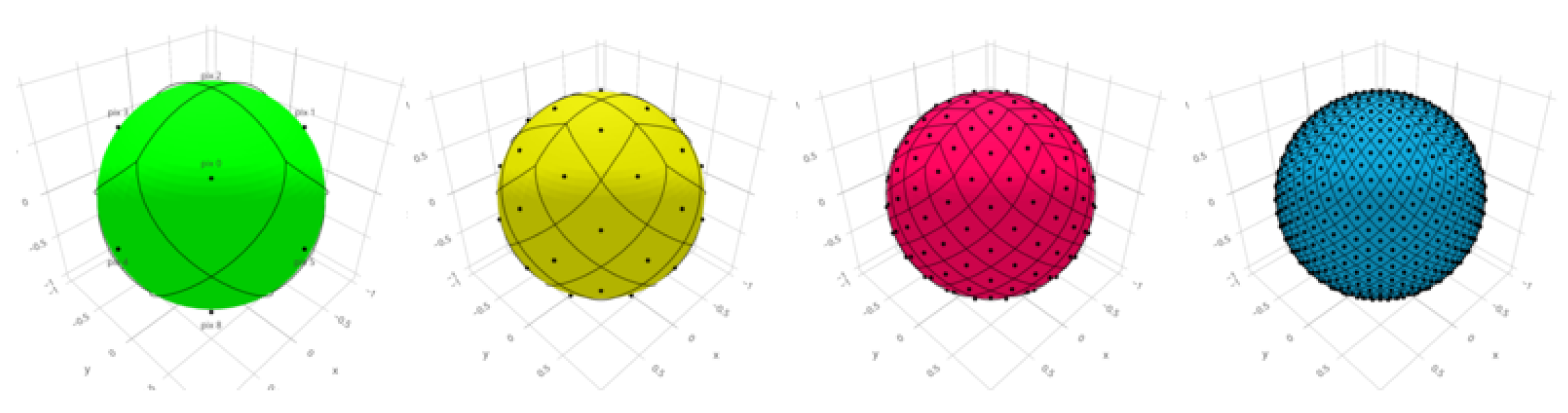
Figure 2.
Heatmap of the space debris density distribution in non-empty pixels for a given time step.
Figure 2.
Heatmap of the space debris density distribution in non-empty pixels for a given time step.
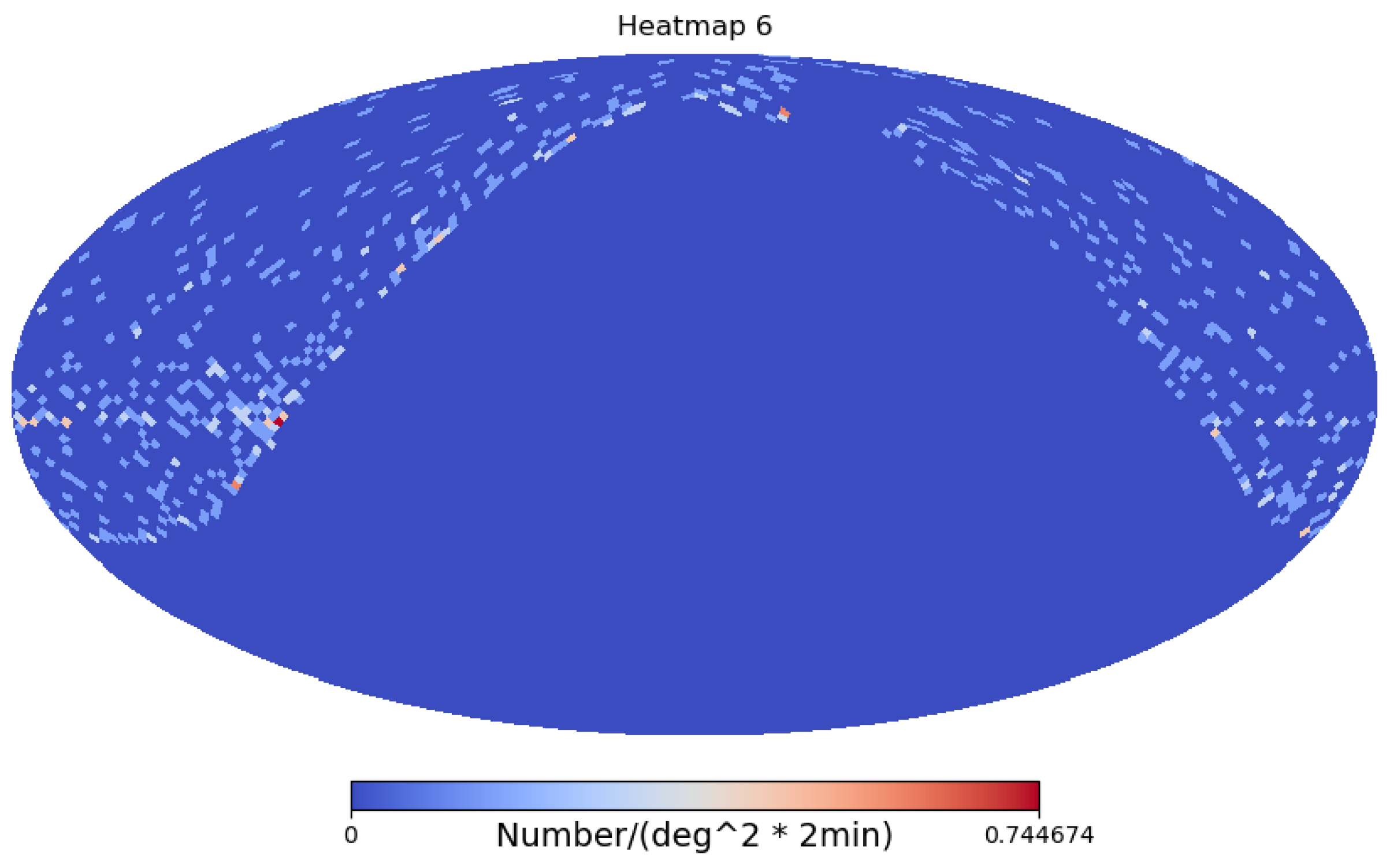
Figure 3.
Density distribution maps of space debris in the observable regions for the first six time steps.
Figure 3.
Density distribution maps of space debris in the observable regions for the first six time steps.
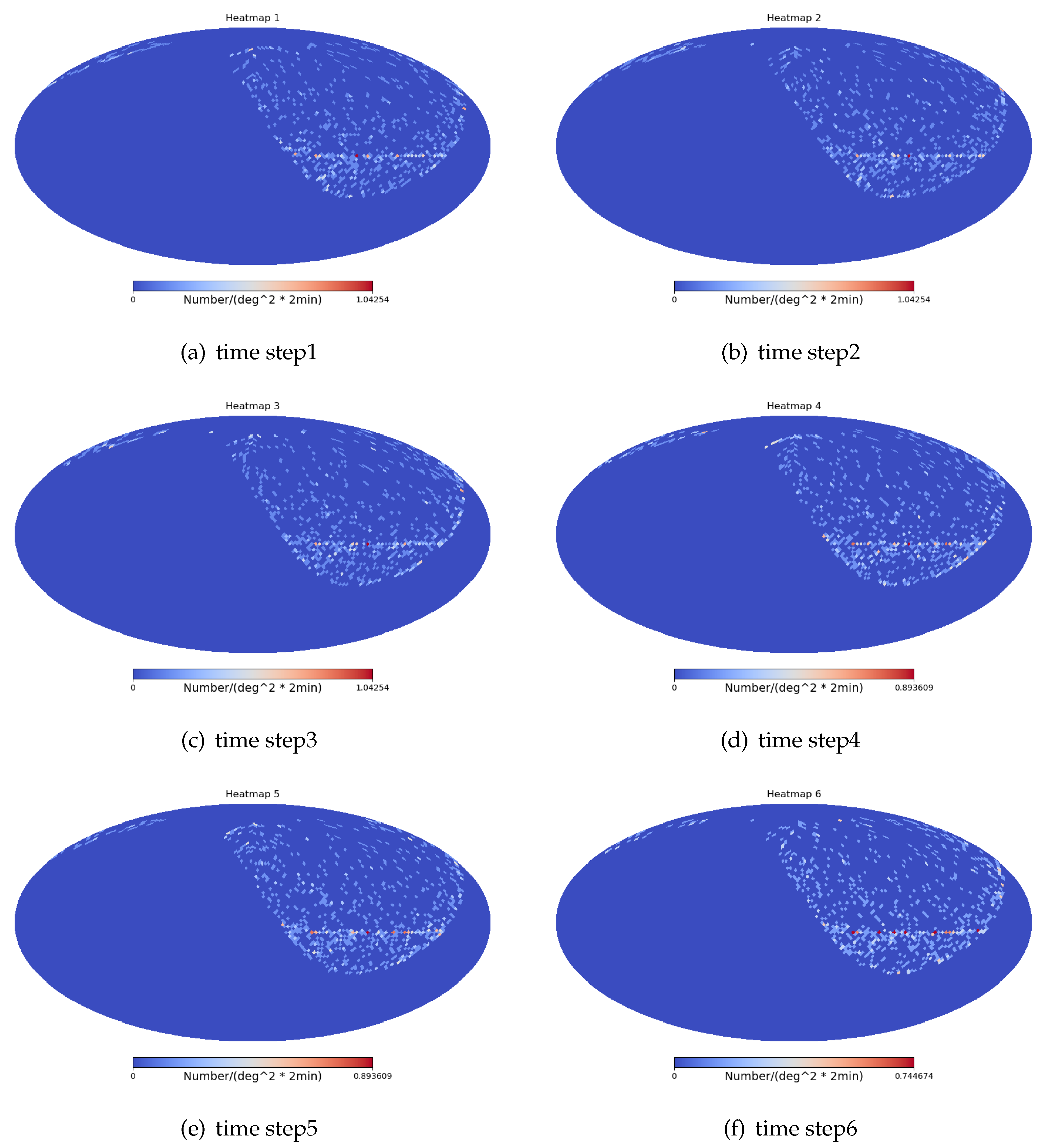
Figure 4.
Schematic of the pointing of the first six time steps of the randomized observation strategy.
Figure 4.
Schematic of the pointing of the first six time steps of the randomized observation strategy.
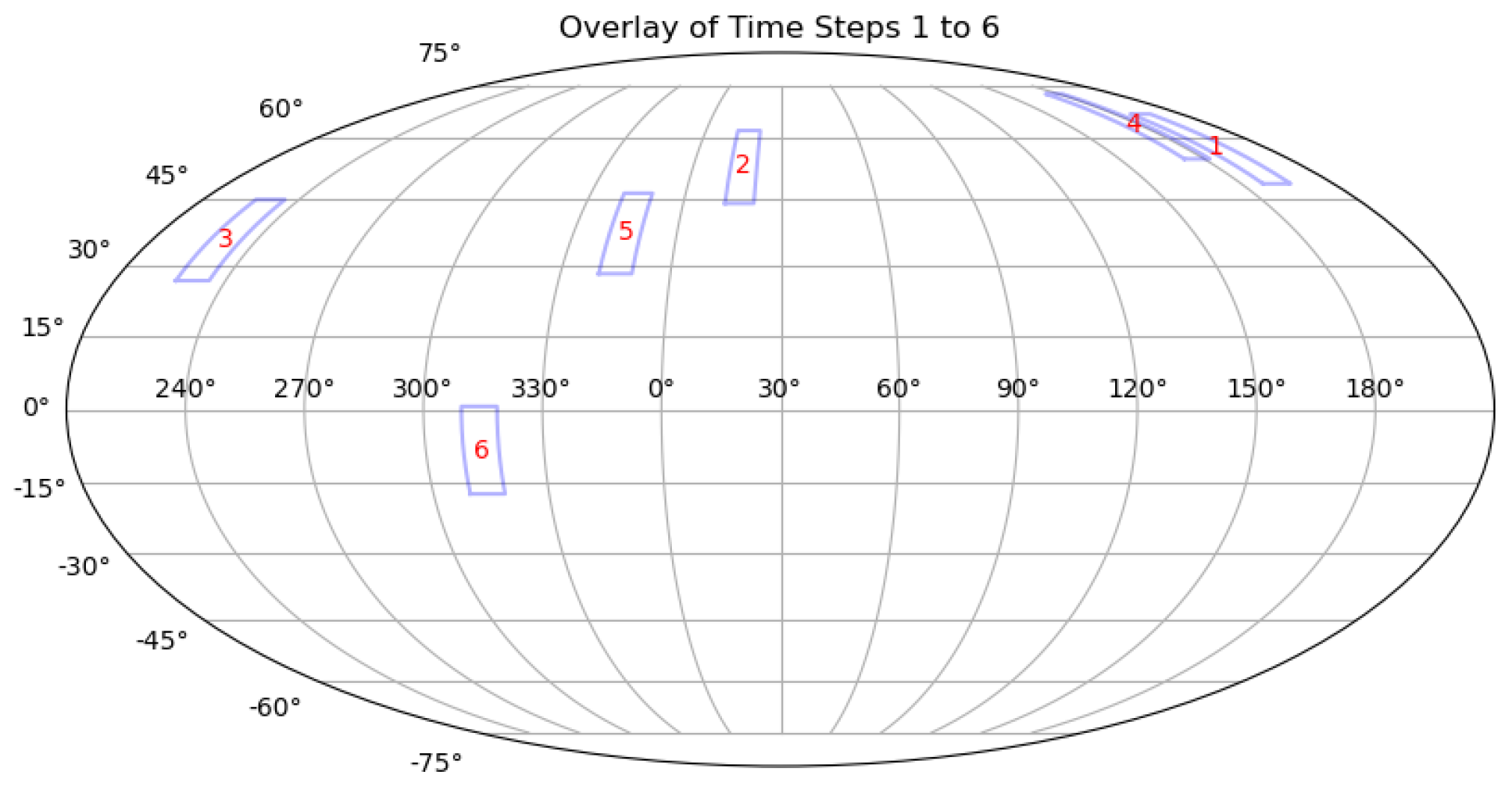
Figure 5.
Schematic of WFOTA pointing with the randomized observation strategy on the night of September 2, 2024.
Figure 5.
Schematic of WFOTA pointing with the randomized observation strategy on the night of September 2, 2024.
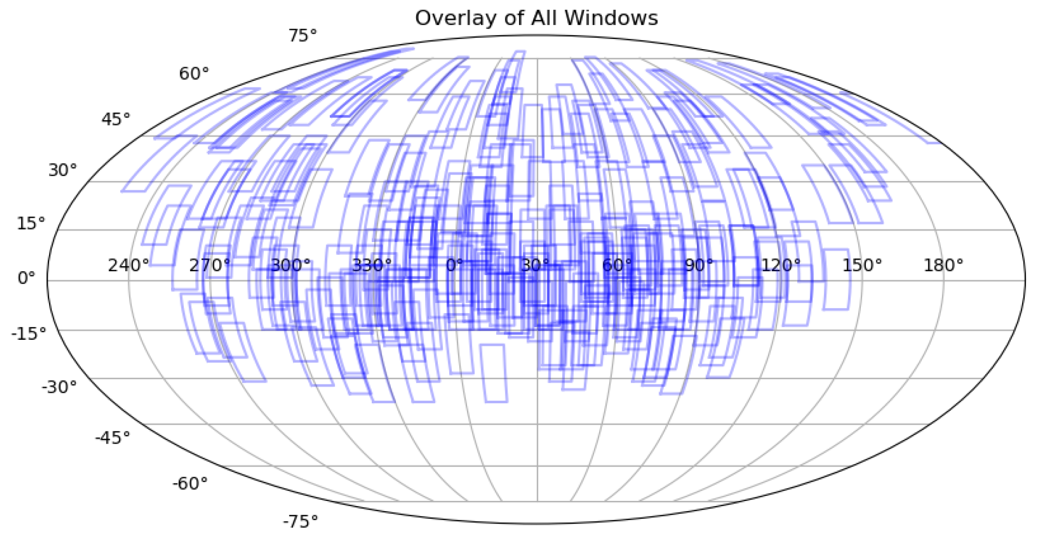
Figure 6.
Schematic of the pointing of the first six time steps of the observation strategy for greedy algorithm.
Figure 6.
Schematic of the pointing of the first six time steps of the observation strategy for greedy algorithm.
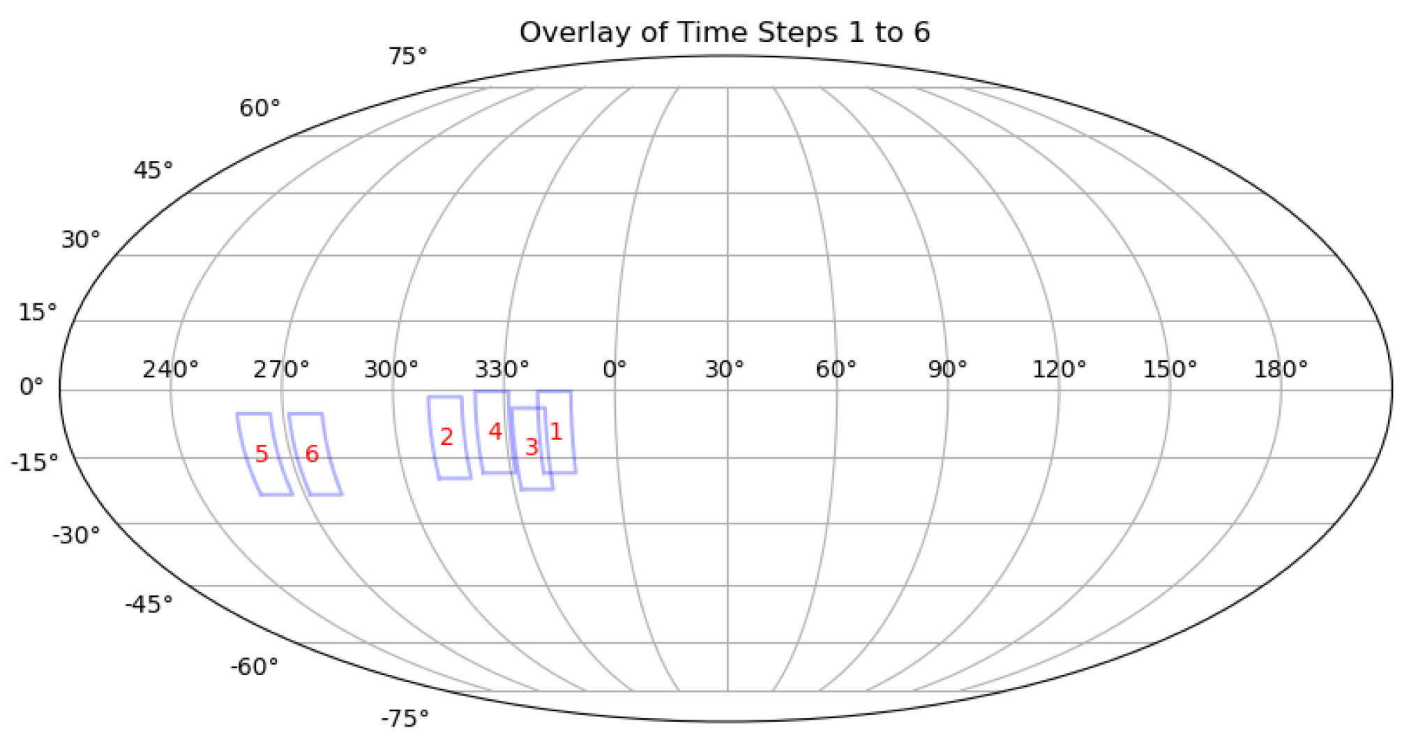
Figure 7.
Schematic of WFOTA pointing with the observation strategy for greedy algorithm on the night of September 2, 2024.
Figure 7.
Schematic of WFOTA pointing with the observation strategy for greedy algorithm on the night of September 2, 2024.
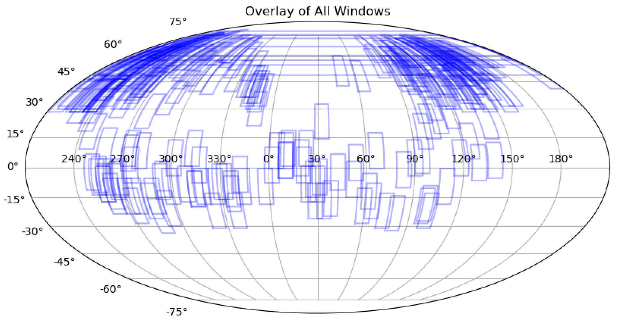
Figure 8.
Schematic of the pointing of the first six time steps of the observation strategy for all-sky coverage.
Figure 8.
Schematic of the pointing of the first six time steps of the observation strategy for all-sky coverage.
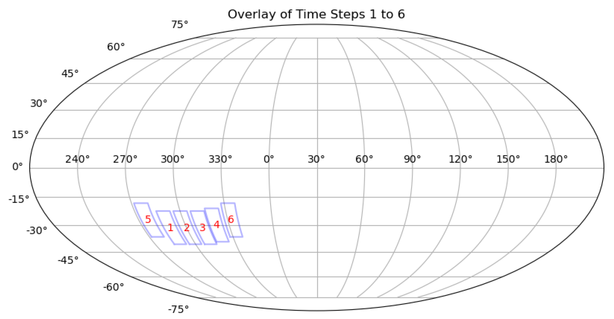
Figure 9.
Schematic of WFOTA pointing with the observation strategy for all-sky coverage on the night of September 3, 2024.
Figure 9.
Schematic of WFOTA pointing with the observation strategy for all-sky coverage on the night of September 3, 2024.
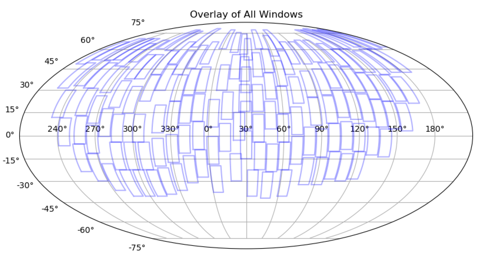

Table 1.
Simulation and observation experiments results of September 2, 2024.
| Telescope Survey Strategy | Observation Strategy for Greedy Algorithm(Arc Segments) | Randomized Observation Strategy(Arc Segments) | Observation Strategy for Greedy Algorithm(Space Debris) | Randomized Observation Strategy(Space Debris) |
|---|---|---|---|---|
| Simulation results | 4579 | 3611 | 3080 | 1505 |
| Observation results | 3455 | 2674 | 331 | 175 |
Table 2.
Simulation and observation experiments results of September 3, 2024.
| Telescope Survey Strategy | Observation Strategy for Greedy Algorithm(Arc Segments) | Observation Strategy for All-Sky Coverage(Arc Segments) | Observation Strategy for Greedy Algorithm(Space Debris) | Observation Strategy for All-Sky Coverage(Space Debris) |
|---|---|---|---|---|
| Simulation results | 4087 | 1125 | 3166 | 904 |
| Observation results | 3058 | 855 | 346 | 94 |
Disclaimer/Publisher’s Note: The statements, opinions and data contained in all publications are solely those of the individual author(s) and contributor(s) and not of MDPI and/or the editor(s). MDPI and/or the editor(s) disclaim responsibility for any injury to people or property resulting from any ideas, methods, instructions or products referred to in the content. |
© 2024 by the authors. Licensee MDPI, Basel, Switzerland. This article is an open access article distributed under the terms and conditions of the Creative Commons Attribution (CC BY) license (http://creativecommons.org/licenses/by/4.0/).
Copyright: This open access article is published under a Creative Commons CC BY 4.0 license, which permit the free download, distribution, and reuse, provided that the author and preprint are cited in any reuse.


