
Submitted:
17 December 2024
Posted:
18 December 2024
You are already at the latest version
Abstract
This paper introduces a team of Automated Guided Vehicles (AGVs) equipped with open-source, perception-enhancing rotating devices. Each device has set of ArUco markers, employed to compute the relative pose of other AGVs. These markers also serve as landmarks, delineating a path for the robots to follow. The authors combined various control methodologies to track the ArUco markers on another rotating device mounted on the AGVs. Behavior trees are implemented to facilitate task-switching or to respond to sudden disturbances, such as environmental obstacles. The Robot Operating System (ROS) is installed on the AGVs to manage high-level controls. The efficacy of the proposed solution is confirmed through a real experiment. This research contributes to the advancement of AGV technology and its potential applications in various fields.
Keywords:
autonomous robots
; multiagent systems
; fiducial marker
; Extended Kalman Filter
; 3D printing
; ROS
; landmarks
; behavior tree
; trajectory tracking
; collision avoidance
1. Introduction
The paper presents a team of Automated Guided Vehicles (AGVs) equipped with open-source, perception-enhancing rotating devices. Each device has 10 ArUco markers, employed to compute the relative pose of other AGVs. Behavior trees are used to rotate the devices on each AGVs. ArUco diamond markers are used as landmarks. Each AGV calculates its own global pose after the detection of the landmarks and also detects the other AGVs in the environment. The goal of task is autonomous localization of multiple robots and also avoiding collisions with other robots in the environment and to reach to their virtual positions. The proposed control is verified using OptiTrack motion capture system providing ground truth in the experimental results.
The paper proposes a novel combination of nonlinear continuous motion control algorithm for robots or AGVs which uses an on-board actuated camera, data fusion (proprioceptive sensors and exteroceptive sensors) and the decision on the direction of perception realized based on behaviour trees to cope with limited computing and sensory resources. In the paper [1] authors proposed actuated camera devices, but it required different hardware configuration for leader and follower robots. The limitation of using different hardware for leader-follower robots is overcome by using proposed hardware [2] by authors which supports any type of robot or AGV’s.
Fiducial markers to which ArUco belongs have become very popular for camera-based positioning. They are often used for comparative studies, e.g. [3,4] and also used in pose estimation experiments [5]. For example, ArUco markers were experimentally compared with other types of markers in [3]. It turned out that their advantages were: good position and orientation results, great detection rate, and low computational cost for single markers. However, they had such disadvantages as: sensitivity to smaller marker sizes and larger distances, computational cost scales with multiple markers.
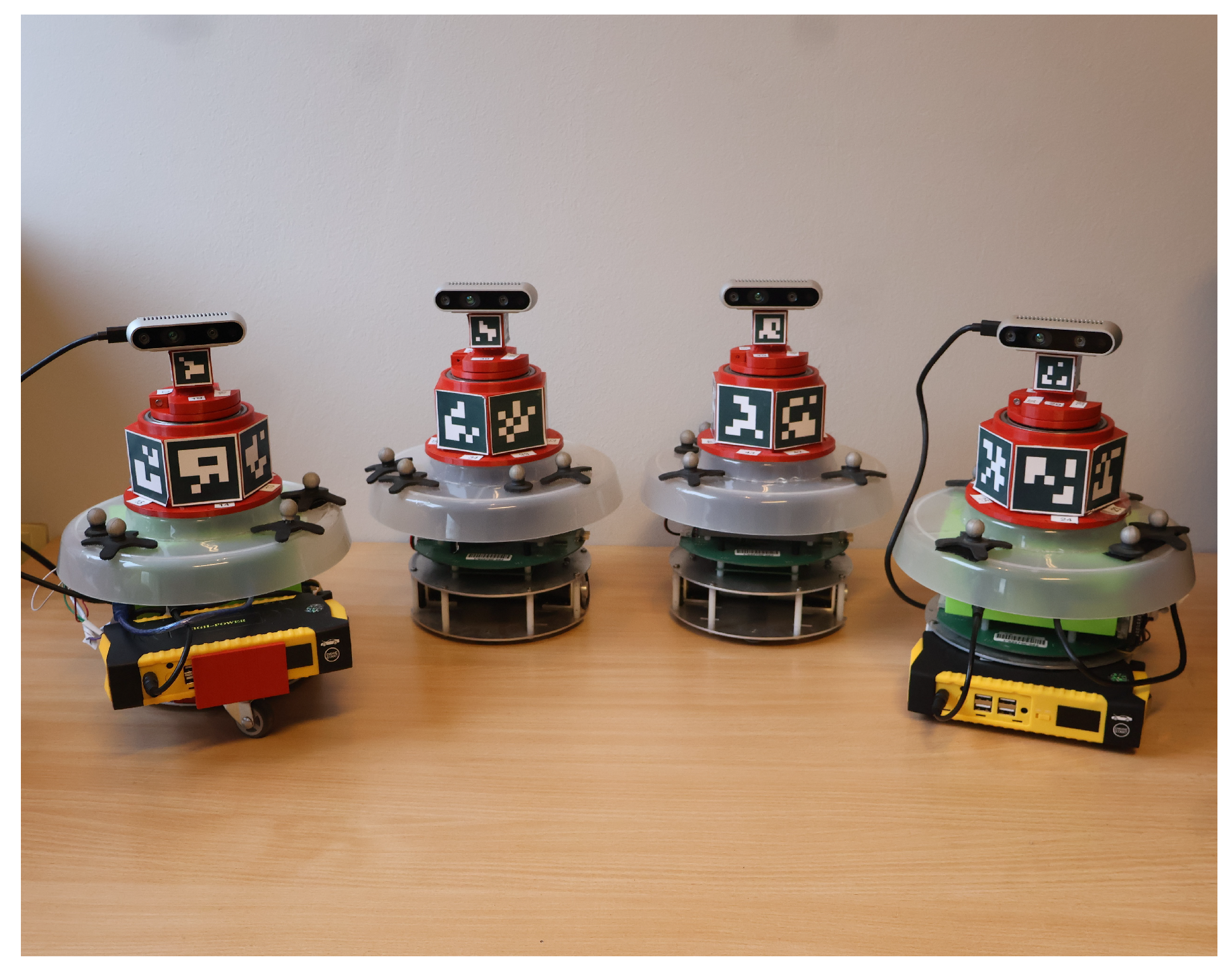
Figure 1.
Robots with rotating platform.
ArUco markers are used in various fields of robotics. Some works on manipulators like [6,7] can be mentioned. Examples of papers on mobile robots in which such a markers were applied are [8,9,10]. Other systems where such markers are useful are flying robots [11,12,13,14,15,16,17]. Markers are also used in cooperative robotics and nuclear decommissioning [18] or to determine the position of a passively cooperating spacecraft [19].
The Extended Kalman Filter (EKF) is used for the localization of an indoor robot [20,21,22,23]. It is also possible to detect cyber attacks using an EKF as shown in [24]. Paper [25] proposes a positioning method for a Magnetic Encoder Guided Vehicle (MEGV) using an EKF. It can also be noted that the neural network EKF is proposed to linearize the output signals [26] or to model unknown disturbances and improve the robot state transition model [27].
The Robot Operating System (ROS) is installed on the AGVs to manage high-level controls. The efficacy of the proposed solution is confirmed through a series of experiments. This research contributes to the advancement of AGV technology and its potential applications in various fields.
The considerations presented in Subsections 2–4 pertain to algorithms operating within the onboard systems of robots based on locally available data. For simplicity, authors have omitted the robot indices. However, it should be noted that they appear N times, corresponding to the number of mobile robots. Only in Subsections 5 and 6 authors introduces indices in the variables to denote the robot numbers, as the algorithm discussed there accounts for the interactions between agents.
An important value of this work is the fact that the presented theoretical considerations were supported by research carried out using a real experiment. Therefore, it can be concluded that the proposed approach to the issues under consideration has undoubted value in laboratory practice involving multi-agent systems. The behavior tree is explained in Section 2. One degree of freedom rotating platform is described in Section 3. Detection of ArUco markers, pose calculation, averaging of ArUco markers, and relative pose between the devices are explained in Section 4. The EKF method is presented in Section 5. All control methods for rotating platforms, collision avoidance techniques, and the kinematic model of robots are explained in Section 6. The methodology of the experiments is explained in Section 7. The experimental results are given in Section 8. The conclusion is discussed in Section 9.
2. Behavior Tree
Behavior trees (BT) are used in computer science, control systems, robotics, and especially in video games. BT is a mathematical model of task execution and the main advantage of BT is to perform complex tasks divided into simple subtasks. The graphical representation of BT is a directed tree consisting of the root node, control nodes, and leaf nodes.
Figure 2 represents the BT for the robot’s rotating platform, which gives the freedom to observe the environment irrespective of the movement of the robot’s mobile platform. Each robot has its own behavior tree. The Python library [28] is used to implement the BT in ROS. The topmost block in Figure 2 represents the root that generates a "tick" signal that propagates through the tree. After the root, the "Sequence 1" node, first sends the tick to the "Look towards Landmarks", the same action node is responsible for moving the rotating platform to look towards the landmarks on the walls for 5 seconds. Control details of the rotating platform are given in Section 6. When the functioning of the block is completed, it sends "SUCCESS" back to the same sequence node, otherwise, it sends "RUNNING". After receiving the "SUCCESS", the next block which is a "Fallback" node is executed. A fallback node works as an "OR" function. When any block below a fallback block gives a "FAILURE" then the other block is executed. The "Sequence 2" node and "Sequence 3" node are under the "Fallback" node. If another robot is detected in the environment in the camera range then the action node "Robot Detected = 1" under the sequence node will give a "SUCCESS" and then the next action node "Look towards Closest Robot" will be executed. The action node "Look towards Closest Robot" will reorient the rotating platform towards the closest robot in the environment around the observing robot. The "Sequence 2" node will send the "FAILURE" to the "Fallback" node when no robot is detected nearby, and then "Sequence 3" is executed, first, it verifies with the action node "Robot Detected = 0". When no robot is detected, the action node "Robot Detected = 0" will give "SUCCESS" and then the "Look straight" node will get a tick, and then the robot will look toward the center of the x-axis of the mobile platform for 5 seconds.
3. Devices for Multi-Agent Systems
The authors have used a one-degree-of-freedom rotating platform designed for multi-agent systems. The device rotates independently from the movement of the mobile platforms of the robot, which is one of its main advantages. Each device was installed on each agent. Figure 3 shows the exploded view of the device. All of its elements were 3D printed. The authors have uploaded the Standard Triangle Language (.stl) file containing models of [29] of the parts. The Fused Deposition Modeling (FDM) 3D printer is used to print these (.stl) files. The PLA (Polylactic Acid) material is used for the 3D printing.
Each device has a total of 10 ArUco markers pasted on it. Part 1 as seen in Figure 3 is of hexagonal shape which has 6 ArUco markers over it of 5x5 dictionary of 5 cm size each and part 3 is of cuboidal shape has 4 ArUco markers over it of 5x5 dictionary of 2.5 cm size. Table 1 shows the mechanical and electronic parts used in the devices.
The dynamixel motor operates from 9 V to 12 V. The motor has a resolution of 0.29 degrees with precise control of position with 1024 steps. As a result, approximately from 0 to 300 degrees [30] comes with feedback. A library [31] is used to connect Arduino Mega to the dynamixel motor. The IC mentioned in Table 1 is used to convert a half-duplex communication to full-duplex communication. The whole device is used as a ROS node, the library [32] is responsible for using the device as a ROS node.
4. ArUco Markers
ArUco markers are squared-shaped fiducial markers and the main advantage is that a single marker is enough to calculate the pose of the camera. A calibrated camera is required to extract the correct pose from the ArUco markers. The distortion matrix D and the camera matrix K of the calibrated camera are as follows:
The Intel RealSense cameras are precalibrated, and the distortion matrix (D) and the camera matrix (K) are taken from the ROS topic of the camera information [33].
4.1. Pose Calculation of ArUco Marker
ArUco markers on the devices have some translation distances from the central axis. To get the center point of one device from another device, virtual rotation and translation are required. OpenCV library [34] for ArUco marker generates the translation , and rotation vectors for each marker when it comes into the camera view frame. Figure 4 shows the representations of the axes between the camera and the ArUco marker. The rotation matrix and the translation matrix are calculated from the translation vector , and rotation vector .
The rotation angle of the rotation vector is:
The rotation vector is normalized as:
The skew-symmetric matrix :
The rotation matrix is calculated as:
where I is the identity matrix. The OpenCV library has a build-in function (Rodrigues) [35] to calculate the directly from rotation vector () to the rotation matrix (camera frame relative to the marker tag) . Now rotation matrix is transformed as follows to change of frames.
To get the center of another device from one device, rotation of the ArUco marker is required before virtual translation towards the center. The aim of the rotation virtually rotate the XY plane of the ArUco marker to make it parallel to the XY plane of the camera. Rotation matrix from Equation (7) is used to calculate the Euler angles (, , ) where , and represents the roll, pitch and yaw of the marker detected in the camera frame.
The rotation matrix to rotate about the y-axis of the ArUco marker is written as:
The new rotation matrix is calculated by multiplying from Equation (8) and rotation matrix from Equation (7):
Now, the distance matrix is added to translation () vector as follows:
where , , in every case and is 4.808 cm when the marker is detected on hexagonal shape (3D printed Part 1) or is 1.5 cm when marker is detected on cubical shape (3D printed Part 3).
- The translation matrix is calculated as follows:
where , , and represent the relative distances from the center of one device to another.
4.2. Averaging of ArUco Marker Measurments
When one device detects another device in the environment, in general more than one ArUco marker is detected in an image frame. All 10 markers on a device should theoretically give the exact center point of the device after virtual rotation and translation, but practically the markers give slightly different measurements. The authors have used the averaging method to obtain one measurement from different markers. Upon detection of the ArUco marker, the OpenCV library [34] also gives the corner points of each marker. Figure 5 shows the corner points of the ArUco markers.
The Shoelace formula [36] is used to calculate the pixel area of each marker which is written as:
where are the x-coordinates of the corner points and represents for y-coordinates of the ArUco marker.
- The total area A is calculated as follows:
Average translation matrix is calculated as follows:
where A is taken from Equation (14), is from Equation (13) and is from Equation (11).
where , , and are the average relative distances from the center of one device to another.
4.3. Relative Pose of One Device to Another
Relative pose of one device to another one is written as follows:
where i represents the device in the environment. As the coordinate frame of the camera and the ArUco marker are different, the distance in the global frame of the x coordinate between the devices will be the distance of the z-axis (, from Equation (16)). Similarly, the global y-coordinate distance of the device is the x-coordinate of ArUco marker from the same Equation (16). The orientation of the device is calculated as follows:
where is the pitch angle calculated from Equation (7), the marker with the largest area is considered, of dynamixel servo motor which is taken from servo feedback. The angle of the observer depends on the relative positions between the devices. Figure 6 shows the top view of the rotating device. Suppose IDs 1 to 6 are pasted in the hexagonal part of the rotating device as shown in Figure 6. Now another observer rotating device is just behind the rotating device placed in Region 1 and looks forward to the center of the device, and it detects the ID 1 on another device then rad as the pose of the ArUco marker also gives the pose of the device itself. In another case where the observer rotating device is in Region 2 and detects ID 2 on another device, rad is added to correct the pose of another detected device. Similarly in another situation is as follows:
- rad in Region 3.
- rad when the pitch angle () is positive for the detected marker (ID4) in Region 4.
- rad when the pitch angle () is negative of the detected marker (ID4) in Region 4.
- rad in Region 5.
- rad in Region 6.
4.4. Pose From Landmarks
Figure 7a shows the image of the ArUco Diamond marker which is used as a landmark in the environment. ArUco Diamond marker structure has 4 markers with size 3 x 3 squares [37,38]. The authors have chosen ArUco Diamond markers as landmarks as the extracted pose information is the average of four ArUco markers on the diamond structure which is more stable as compared to single ArUco markers. Figure 7b shows the environment with 5 landmarks. Different IDs of ArUco markers are selected to differentiate between markers.
Each landmark in the environment gives the robot its global pose after modification in extracted pose from the detected ArUco diamond in the frame. Figure 4 also shows the axis representations between the camera and the ArUco Diamond markers, as they are the same as those of the single ArUco marker. The rotation vector () and the translation vector are () of the ArUco Diamond marker extracted by the OpenCV library [38] once detected in the camera frame where denotes the landmark number ().
The rotation matrix () is calculated from () using the built-in function (Rodrigues) [35] and after translation () the rotating matrix is written as:
The new translation matrix () is calculated by adding some translation distance in the y-axis of the markers which is expressed as follows:
where , the value of are given in Section 8.
The translation matrix is calculated as follows:
The vector represents the distance from the landmarks and is written as:
The rotation matrix from Equation (19) is used to calculate the Euler angles (, , ) where , and represents the roll, pitch, and yaw of the landmark detected in the camera frame. The global pose of the robot in the environment is written:
5. Extended Kalman Filter
The aim of the EKF is to localize the robot in the environment using the data coming from the encoder and the global pose from the landmarks. EKF model is taken from the paper [39]. The state vector of the system of EKF is written as:
where r represents the robot and represents the pose expressed in the global coordinate frame. Linear velocity and angular velocity are represented as and , respectively.
The discrete-time model of the system is written as follows:
The state model Equation (26) and measurement model Equation (27) of the filter are as follows:
where represents the nonlinear system and represents the measurement model. The represents the Gaussian noise of the dynamic system and represents the Gaussian noise of the measurement. Both noise and are zero mean Gaussian noise and associated with covariance matrices are and as:
The nonlinear function and is to be linearized to obtain the linearized model of the system. A Jacobian matrix of and at the operating point is calculated as:
The prediction equations are as follows:
The update equations are as follows:
where represents the Kalman gain, and are estimates of the a priori and a posteriori state.
5.1. Measurement model
The Subsection 5.1.1 explains the calculation of linear () and angular () velocities of the robot from the wheel encoders. The other subsection 5.1.2 explains the use of the global pose in the EKF of the robot after the detection of the landmark.
5.1.1. Data from wheel encoders
All robots are equipped with encoders on their motors. The wheel angular velocities of the left and right wheels are expressed as:
where angular velocities (rad/s) are of the left wheel and of the right wheel of the r-th robot. The current encoder ticks and previously saved encoder ticks for the left wheel and right wheel are , and and respectively. The time between the two consecutive readings of the readings of the left and right wheels are and , respectively.
The linear velocities of wheels is calculated by multiplying wheel radius to Equations (37) and (38) as:
Equations (39) and (40) are used to calculate the linear and angular velocities of robots as follows:
where the robot’s length of the wheel separation is . and are the linear and angular velocities of the robots calculated from the readings of the wheels encoders.
The measurement matrix is written as:
The matrix is as follows:
5.1.2. Landmark Data
After the detection of the landmarks by the robot camera matrix from Equation (23) gives the global pose of the robot. The direct angle from the landmark is not considered as the robots are equipped with the rotating platform. The calculation of the angle from the landmark is written as:
where is the robot orientation, is the angle generated from the landmark detection and is the third component taken from Equation (23) and is the angle of the rotating platform of the robot. depends on the specific position of the robot. The values of are given in Section 8.
of the landmark is as follows:
where as , are taken from Equation (23).
The matrix is as follows:
6. Controls
6.1. Controls of Rotating Device
The rotating device tracks the ArUco markers on another rotating device by the PID controller. The main aim is to minimize the distance between the center of the camera and the ArUco marker as minimum as possible. The distance between the center of the ArUco marker and the camera center () is taken from Equation (12) or (16) depending on the case of the ArUco marker.
Where is the control signal generated for a time t. , and are the proportional gain, integral gain, and derivative gain parameters, is the change in error, is the change in time, is expressed as follows:
where is the set point that is set to zero as the camera should point in the middle of the ArUco marker. is the current angle of the rotating platform of the robot.
6.2. Collision Avoidance
The collision avoidance used in this paper is the idea presented by [40] and later widely used in multi-agent systems [41,42,43,44,45].
The robot r avoids collisions with all other robots j, using Artificial Potential Function (APF). All robots are surrounded by APFs that raise to infinity near the robot’s/obstacle’s boundary, - radius of the robot (j - number of the robot/obstacle), and monotonically decrease to zero at some radius , .
The APF [44] is written as :
the above function gives the output .
The Euclidean length is used to calculate the distance between r-th robot and the j-th obstacle (or robot) .
To scale the function (50) within the range , the following equation is used:
The scalar function , is used in control to generate collision avoidance behaviors by using its spatial partial derivatives. The approach outlined above is also used to avoid collisions with a static obstacle with the center located at point , with radius and APF vanishing at distance from the center. In this case, all the above equations remain valid if o is substituted in place of j.
6.3. Control of Mobile Platform
Each moving robot has its own virtual robot which acts as a leader robot. The kinematic model of the mobile robots is written as:
where , , represent the robot’s pose in the global reference frame. represents the control vector where the linear velocity is and represents the controls of the angular velocity of the robot, respectively.
The following global quantities to zero:
where , and represent the components of the pose of the virtual robot (). , and and are taken from the robot EKF system, Equation (35). Now the system errors with respect to the robot’s fixed frame is as follows:
Adding the collision avoidance components
The gradient of the APF can be expressed with respect to the local coordinate frame fixed to the r-th robot:
The above equations is re-written as follows:
Due to its simplicity and its effectiveness, the trajectory tracking algorithm is taken from [46]. The control for i-th robot is written as:
where is the desired velocities vector of the virtual robot where is the linear velocity and is the angular velocity. , and are constant parameters greater then zero and function is defined as follows:
The detailed analysis of the properties of the control for a single platform without collision avoidance is presented in paper [47].
7. Methodology
The experiment is carried out with four real robots which are shown in Figure 1. All robots are equipped with an Intel NUC where ROS Noetic is deployed. Each robot has its own controller in its own NUC system which works totally independently from each other. Low-level controllers are present in each robot which works as ROS nodes. The low-level controller subscribes to robot linear and angular velocities and publishes the ticks from the encoder. All robots are connected to one WiFi router to have access to roscore. One PC is also connected to the same WiFi router to launch roscore. The robots in the environment work as slaves to the ROS master. In the environment, landmarks are pasted on the vertical surface as seen in Figure 7b.
Two robots worked as static obstacles in the experiment. The other two robots move in the environment to avoid the static robots in the environment and try to reach their virtual robot’s localization. With the use of behavior trees moving robots watch towards the landmarks for 5 seconds and watch towards the closest robot or in a straight moving direction.
8. Experimental Results
The experiment video is uploaded on online platform [https://youtu.be/rDvpCEM7DmE]. Robots Numbers 1 and 2 are moving in the environment. Both the Robots number 1 and 2 have to follow their virtual robot 1 and virtual robot 2 respectively. The experiment is done for 60 seconds. The starting pose and end pose of virtual robot 1 are m and m, respectively, and for virtual robot 2 they are m and m. The virtual robots have to generate a straight path. The desired velocities for both virtual robots are m/s. The values of and of APF in the collision avoidance section 6.2 are considered to be m, m, respectively. of Equation (20) is considered as when the landmark number 1 in the environment detected by the robot in Figure (7b) then , for other landmarks , , and . in Equation (20) are the distance between the landmark 1 to other markers in the environment. of Equation (45) is considered in two cases. In case 1 is when the robot moves toward the positive x-axis of the environment and the rotating platform is watching toward the landmarks on the wall which are on the positive y-axis of the environment, then . In case 2 is when the robot moves toward a negative x-axis and the rotating platform observes the landmarks on the wall that are on the positive y-axis of the environment, then . The constant parameters of the controller Equation (63) are considered as , and .
Figure 8a shows the path for virtual robots 1 and 2, the calculated EKF path of robots 1 and 2, and the Opti-track path for all four robots. Figure 8b shows the -plot of robot 1 with static robot 4 with activation region. Figure 8c shows the -plot of robot 2 with virtual robot 2. Figure 8d shows the -plot of all robots with activation regions. The collision avoidance components and of robot 1 are shown in Figure 8e and Figure 8f respectively. The global errors of the robot, 1 on the x axis, y axis, and with with respect to time, are shown in Figure 8g, Figure 8h and Figure 8i respectively. The linear and angular velocities of robot 1 with respect to time are shown in Figure 8j and Figure 8k.
The collision avoidance components and of robot 2 are shown in Figure 8l and Figure 8m respectively. The global errors of the robot 2 in x axis, y axis and with with respect to time is shown in Figure 8n, Figure 8o and Figure 8p respectively. The linear and angular velocities of robot 2 with respect to time are shown in Figure 8q and Figure 8r.
Figure 8t and Figure 8v show the detections of other robots in the environment by robot 1 and robot 2 respectively. The detection of landmarks by robot 1 and robot 2 is shown in Figure 8s and Figure 8u.
The ground truth from the OptiTrack is used to evaluate the results from on-board measurements. The OptiTrack paths for Robots 1 and 2 are in the range of approximately m with the EKF path generated for robots as seen in Figure 8a. It should be seen as a goal that was reached in this work.
9. Conclusions
The paper shows the algorithm that uses open-source rotating devices installed on all robots. The movement of the devices is independent of the movement of the robot’s mobile platform. Rotating devices are capable of detecting other rotating devices installed on robots in the environment and are also capable of detecting landmarks in the environment. Behavior trees are used to change the orientation of the camera towards the location of landmarks and towards the closest robot or to look straight towards the moving axis. An experiment was performed with four robots, two robots were stationary and worked as static obstacles in the environment. The other two robots were following their virtual robots’ trajectories and avoid collisions with other robots present in the environment. An Extended Kalman Filter is used to localize the robots from the data coming from encoders and from landmarks. The global pose of the robot is calculated and updated after the detection of the landmarks. The proposed research method was verified by an actual experiment, which confirms its usefulness in laboratory practice related to testing multi-agent systems.
Author Contributions
Conceptualization, A.J. and P.H.; Methodology, A.J. and W.K.; Software, A.J. and W.K.; Investigation, P.H.; Resources, W.K.; Writing—original draft, A.J. and W.K.; Writing—review & editing, W.K. and P.H.; Supervision, W.K. and P.H. All authors have read and agreed to the published version of the manuscript.
Funding
This paper was supported by statutory grant 0211/SBAD/0123 and faculty grant 0211/SBAD/0424.
Data Availability Statement
The original contributions presented in this study are included in the article. Further inquiries can be directed to the corresponding author.
Conflicts of Interest
The authors declare no conflict of interest.
References
- Joon, A.; Kowalczyk, W. Leader–Follower Approach for Non-Holonomic Mobile Robots Based on Extended Kalman Filter Sensor Data Fusion and Extended On-Board Camera Perception Controlled with Behavior Tree. Sensors 2023, 23, 8886. [Google Scholar] [CrossRef]
- A. Joon and W. Kowalczyk, "An Open-Source Rotating Device for Relative Localization in Multi-Agent Systems," 2024 13th International Workshop on Robot Motion and Control (RoMoCo), Poznań, Poland, 2024, pp. 69-75. [CrossRef]
- Kalaitzakis, M.; Cain, B.; Carroll, S.; Ambrosi, A.; Whitehead, C.; Vitzilaios, N. Fiducial Markers for Pose Estimation Overview, Applications and Experimental Comparison of the ARTag, AprilTag, ArUco and STag Markers. Journal of Intelligent & Robotic Systems 2021, 101, 71. [Google Scholar]
- Jurado-Rodriguez, D.; Munoz-Salinas, R.; Garrido-Jurado, S.; Medina-Carnicer, R. Design, Detection, and Tracking of Customized Fiducial Markers. IEEE Access 2021, 9, 140066–140078. [Google Scholar] [CrossRef]
- Cepon, G.; Ocepek, D.; Kodric, M.; Demsar, M.; Bregar, T.; Boltezar, M. Impact-Pose Estimation Using ArUco Markers in Structural Dynamics. Experimental Techniques 2024, 48, 369–380. [Google Scholar] [CrossRef]
- Hayat, A.A.; Boby, R.A.; Saha, S.K. A geometric approach for kinematic identification of an industrial robot using a monocular camera. Robotics and Computer Integrated Manufacturing 2019, 57, 329–346. [Google Scholar] [CrossRef]
- Balanji, H.M.; Turgut, A.E.; Tunc, L.T. A novel vision-based calibration framework for industrial robotic manipulators. Robotics and Computer-Integrated Manufacturing 2022, 73. [Google Scholar] [CrossRef]
- Botta, A.; Quaglia, G. Performance Analysis of Low-Cost Tracking System for Mobile Robots. Machines 2020, 8, 29. [Google Scholar] [CrossRef]
- Roos-Hoefgeest, S.; Garcia, I.A.; Gonzalez, R.C. Mobile robot localization in industrial environments using a ring of cameras and ArUco markers. In Proceedings of IECON 2021 - 47th Annual Conference of the IEEE Industrial Electronics Society, Toronto, ON, Canada, 2021, pp. 1-6.
- Babinec, A.; Jurisica, L.; Hubinsky, P.; Duchon, F. Visual localization of mobile robot using artificial markers. Procedia Engineering 2014, 96, 1–9. [Google Scholar] [CrossRef]
- Miranda, V.R.F.; Rezende, A.M.C.; Rocha, T.L.; Azpurua, H.; Pimenta, L.C.A.; Freitas, G.M. Autonomous Navigation System for a Delivery Drone. Journal of Control, Automation and Electrical Systems 2022, 33, 141–155. [Google Scholar] [CrossRef]
- Xing, B.; Zhu, Q.; Pan, F.; Feng, X. Marker-Based Multi-Sensor Fusion Indoor Localization System for Micro Air Vehicles. Sensors 2018, 18, 1706. [Google Scholar] [CrossRef] [PubMed]
- Morales, J.; Castelo, I.; Serra, R.; Lima, P.U.; Basiri, M. Vision-Based Autonomous Following of a Moving Platform and Landing for an Unmanned Aerial Vehicle. Sensors 2023, 23, 829. [Google Scholar] [CrossRef]
- Wubben, J.; Fabra, F.; Calafate, C.T.; Krzeszowski, T.; Marquez-Barja, J.M.; Cano, J.-C.; Manzoni, P. Accurate Landing of Unmanned Aerial Vehicles Using Ground Pattern Recognition. Electronics 2019, 8, 1532. [Google Scholar] [CrossRef]
- Liu, S.; Fantoni, I.; Chriette, A. Decentralized control and state estimation of a flying parallel robot interacting with the environment. Control Engineering Practice 2024, 144, 105817. [Google Scholar] [CrossRef]
- Zhong, Y.; Wang, Z.; Yalamanchili, A.V.; Yadav, A.; Ravi Srivatsa, B.N.; Saripalli, S.; Bukkapatna, S.T.S. Image-based flight control of unmanned aerial vehicles (UAVs) for material handling in custom manufacturing. Journal of Manufacturing Systems 2020, 56, 615–621. [Google Scholar] [CrossRef]
- Bacik, J.; Durovsky, F.; Fedor, P.; Perdukova, D. Autonomous flying with quadrocopter using fuzzy control and ArUco markers. Intelligent Service Robotics 2017, 10, 185–194. [Google Scholar] [CrossRef]
- Burrell, T.; West, C.; Monk, S.D.; Montezeri, A.; Taylor, C.J. Towards a Cooperative Robotic System for Autonomous Pipe Cutting in Nuclear Decommissioning. In Proceedings of 2018 UKACC 12th International Conference on Control (CONTROL) Sheffield, UK, 5-7 Sept 2018, pp.283–288.
- Vela, C.; Fasano, G.; Opromolla, R. Pose determination of passively cooperative spacecraft in close proximity using a monocular camera and AruCo markers. Acta Astronautica 2022, 201, 22–38. [Google Scholar] [CrossRef]
- Qian, J.; Zi, B.; Wang, D.; Ma, Y.; Zhang, D. The Design and Development of an Omni-Directional Mobile Robot Oriented to an Intelligent Manufacturing System. Sensors 2017, 17, 2073. [Google Scholar] [CrossRef]
- Zhang, L.; Wu, X.; Gao, R.; Pan, L.; Zhang, Q. A multi-sensor fusion positioning approach for indoor mobile robot using factor graph. Measurement 2023, 216, 112926. [Google Scholar] [CrossRef]
- Rekleitis, I.; Meger, D.; Dudek, G. Simultaneous planning, localization, and mapping in a camera sensor network. Robotics and Autonomous Systems 2006, 54, 921–932. [Google Scholar] [CrossRef]
- Zhou, G.; Luo, J.; Meng, S. An EKF-based multiple data fusion for mobile robot indoor localization. Assembly Automation 2021, 41(3), 274–282. [Google Scholar] [CrossRef]
- Guo, J.; Li, L.; Wang, J.; Li, K. Cyber-Physical System-Based Path Tracking Control of Autonomous Vehicles Under Cyber-Attacks. IEEE Transactions on Industrial Informatics 2023, 19(5), 6624–6635. [Google Scholar] [CrossRef]
- Cho, H.; Kim, E.K.; Jang, E.; Kim, S. Improved Positioning Method for Magnetic Encoder Type AGV Using Extended Kalman Filter and Encoder Compensation Method. International Journal of Control, Automation and Systems 2017, 15, 1844–1856. [Google Scholar] [CrossRef]
- Mekonnen, G.; Kumar, S.; Pathak, P.M. Wireless hybrid visual servoing of omnidirectional wheeled mobile robots. Robotics and Autonomous Systems 2016, 75, 450–462. [Google Scholar] [CrossRef]
- Miljkovic, Z.; Vukovic, N.; Mitic, M.; Babic, B. New hybrid vision-based control approach for automated guided vehicles. The International Journal of Advanced Manufacturing Technology 2013, 66, 231–249. [Google Scholar] [CrossRef]
- Py-trees. Available online: https://pypi.org/project/py-trees/ (accessed on 30 Nov 2024).
- Open Source Rotating Platform for Multi-agent Mobile Robots. Available online: https://www.thingiverse.com/thing:6550991 (accessed on 30 May 2024).
- Dynamixel e-Manual. Available online: https://emanual.robotis.com/docs/en/dxl/ax/ax-12a/ (accessed on 22 February 2024).
- NeuroRoboticTech/DynamixShield. Available online: https://github.com/NeuroRoboticTech/Dynamix Shield/tree/master/libraries/DynamixelSerial (accessed on 22 February 2024).
- rosserial arduino/Tutorials - ROS Wiki. Available online: https://wiki.ros.org/rosserial_arduino/Tutorials (accessed on 22 February 2024).
- ROS Wrapper for Intel. Available online: https://github.com/IntelRealSense/realsense-ros (accessed on 2 June 2024).
- Detection of ArUco Markers. Available online: https://docs.opencv.org/4.x/d5/dae/tutorial_aruco_detection.html (accessed on 2 June 2024).
- Camera Calibration and 3D Reconstruction - OpenCV. Available online: https://docs.opencv.org/2.4/modules/calib3d/doc/camera_calibration_and_3d_reconstruction.html?highlight=camera%20calibration#rodrigues (accessed on 2 June 2024).
- Braden, B. The Surveyor’s Area Formula. The College Mathematics Journal 1986, 17, 326–337. [Google Scholar] [CrossRef]
- Camera posture estimation using an ARUCO diamond marker. Available online: https://longervision.github.io/2017/03/11/ComputerVision/OpenCV/opencv-external-posture-estimation-ArUco-diamond/ (accessed on 30 November 2024).
- Charuco Diamond Creation. OpenCV. Available online: https://docs.opencv.org/4.x/d5/d07/tutorial_charuco_diamond_detection.html (accessed on 1 December 2024).
- Al Khatib, E.I.; Jaradat, M.A.K.; Abdel-Hafez, M.F. Low-Cost Reduced Navigation System for Mobile Robot in Indoor/Outdoor Environments. IEEE Access 2020, 8, 25014–25026. [Google Scholar] [CrossRef]
- Khatib, O. Real-time Obstacle Avoidance for Manipulators and Mobile Robots,Int. J. Robot. Res. 1986, 5, 90–98. [Google Scholar] [CrossRef]
- Mastellone, S.; Stipanovic, D.; Spong, M. Formation control and collision avoidance for multi-agent non-holonomic systems: Theory and experiments. Int. J. Robot. Res. 2008, 107–126. [Google Scholar] [CrossRef]
- Do, K.D. Formation Tracking Control of Unicycle-Type Mobile Robots With Limited Sensing Ranges, IEEE Trans. Control Syst. Technol. 2008, 16, 527–538. [Google Scholar] [CrossRef]
- Kowalczyk, W.; Kozłowski, K.; Tar, J.K. Trajectory Tracking for Multiple Unicycles in the Environment with Obstacles. In Proceedings of the 19th International Workshop on Robotics in Alpe-Adria-Danube Region (RAAD 2010), Budapest, Hungary, 23–27 June 2010; pp. 451–456. [Google Scholar] [CrossRef]
- Kowalczyk, W.; Michałek, M.; Kozłowski, K. Trajectory Tracking Control with Obstacle Avoidance Capability for Unicycle-like Mobile Robot. Bull. Pol. Acad. Sci. Tech. Sci. 2012, 60, 537–546. [Google Scholar] [CrossRef]
- Kowalczyk, W.; Kozłowski, K. Leader-Follower Control and Collision Avoidance for the Formation of Differentially-Driven Mobile Robots. In Proceedings of the MMAR 2018—23rd International Conference on Methods and Models in Automation and Robotics, Miedzyzdroje, Poland, 27–30 August 2018. [Google Scholar]
- Tsoukalas, A.; Tzes, A.; Khorrami, F. Relative Pose Estimation of Unmanned Aerial Systems,2018 26th Mediterranean Conference on Control and Automation (MED), Zadar, Croatia, 2018, pp. 155-160, doi: 10.1109/MED.2018.8442959. [CrossRef]
- C. Canudas de Wit, H. Khennouf, C. Samson, O. J. Sordalen, Nonlinear Control Design for Mobile Robots. Recent Trends Mob. Rob. 1994, 121–156. [CrossRef]
Figure 2.
Behavior Tree for rotating platform movement.
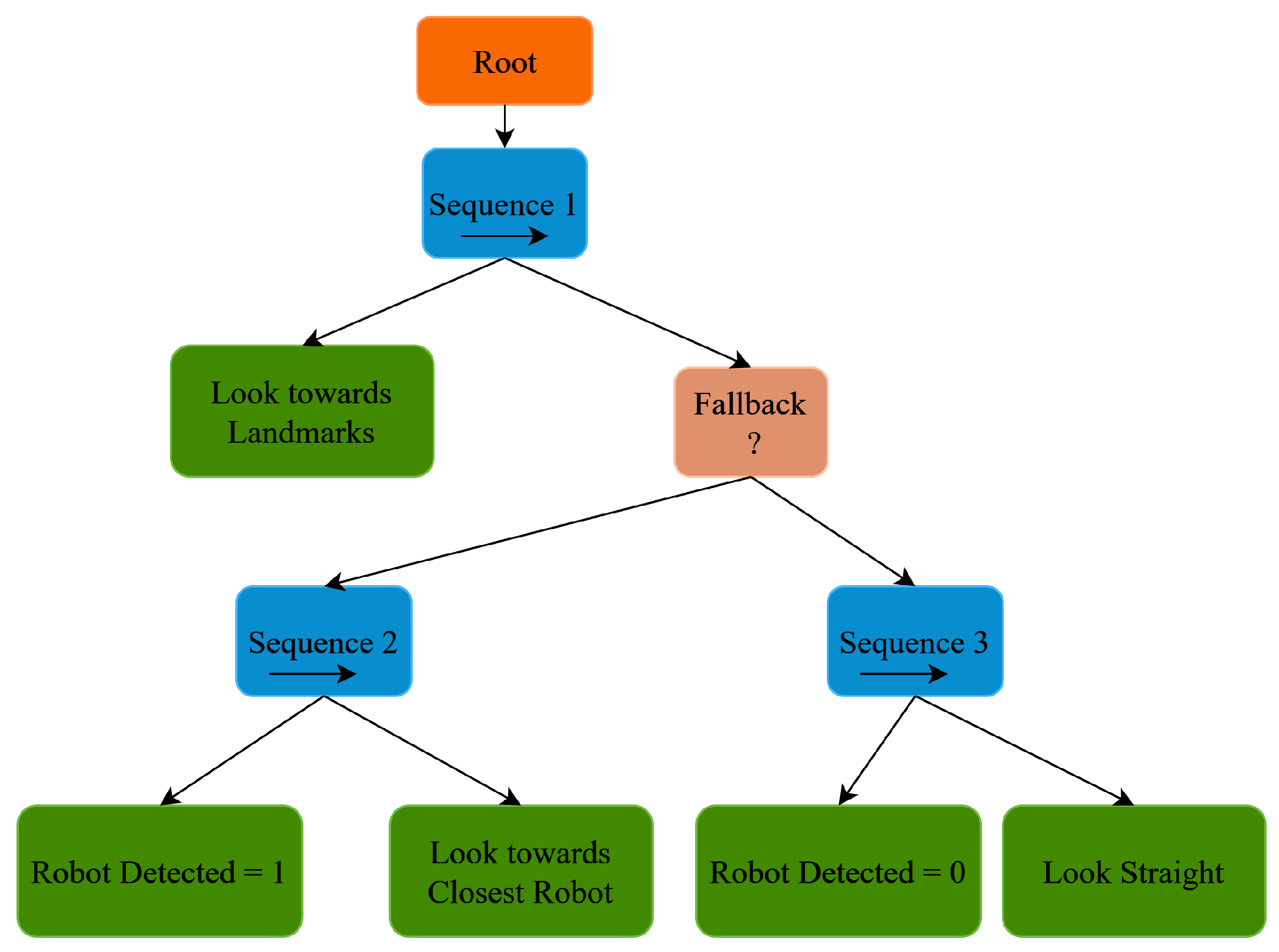
Figure 3.
Exploded view of assembly.
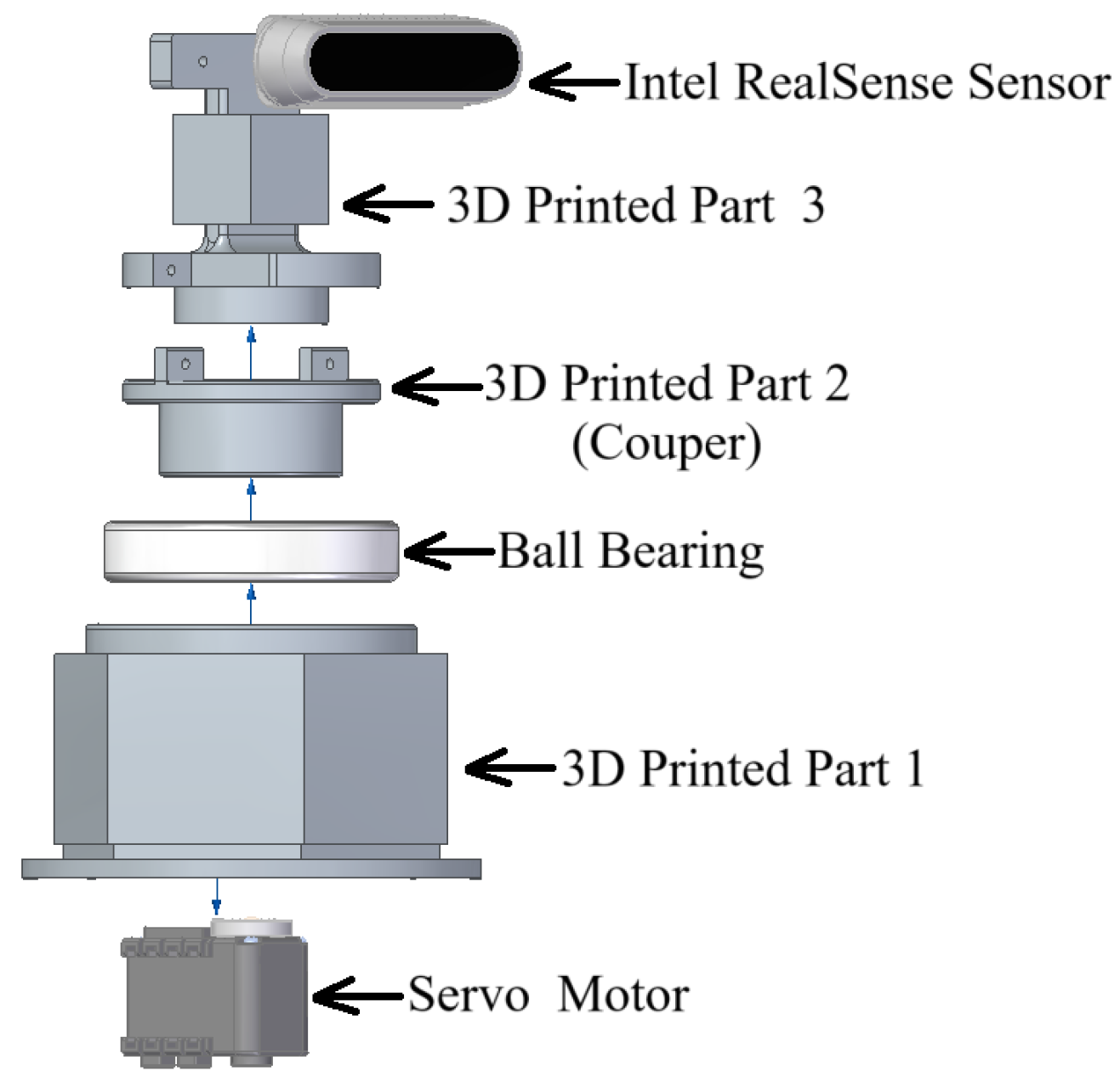
Figure 4.
Axis representations between the camera and the ArUco marker.
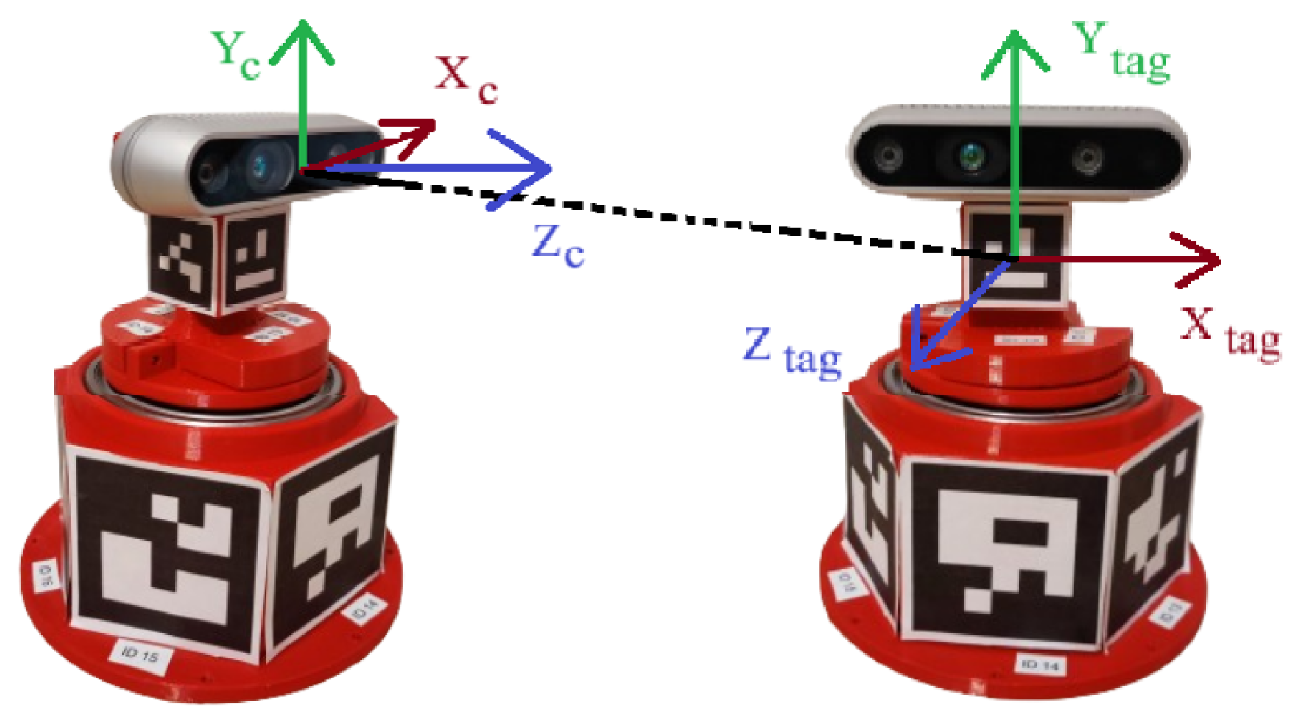
Figure 5.
Corner points of ArUco marker.
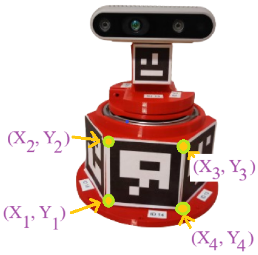
Figure 6.
Top view of the rotating device.
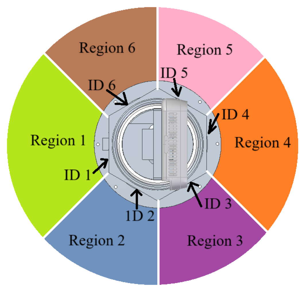
Figure 7.
Side-by-side comparison of (a) ArUco Diamond Marker and (b) Environment with landmarks.
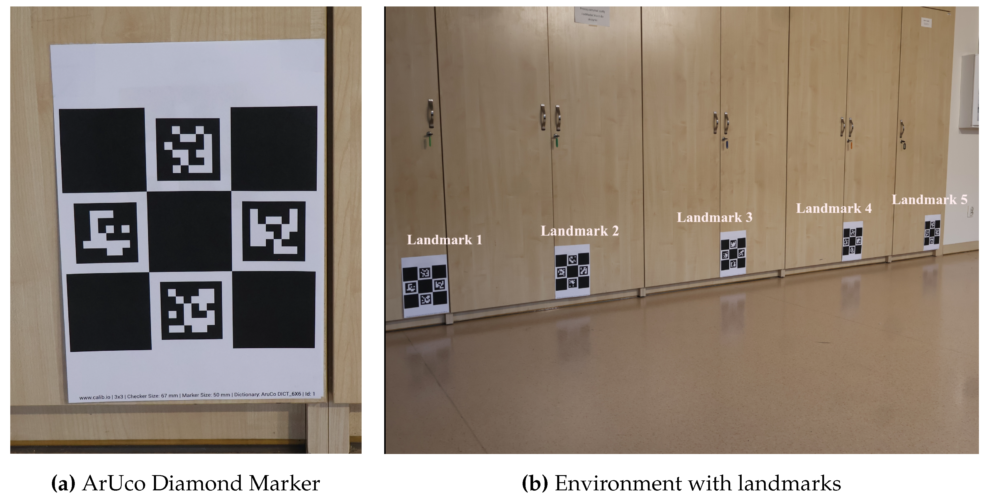
Figure 8.
Experiment result 1.
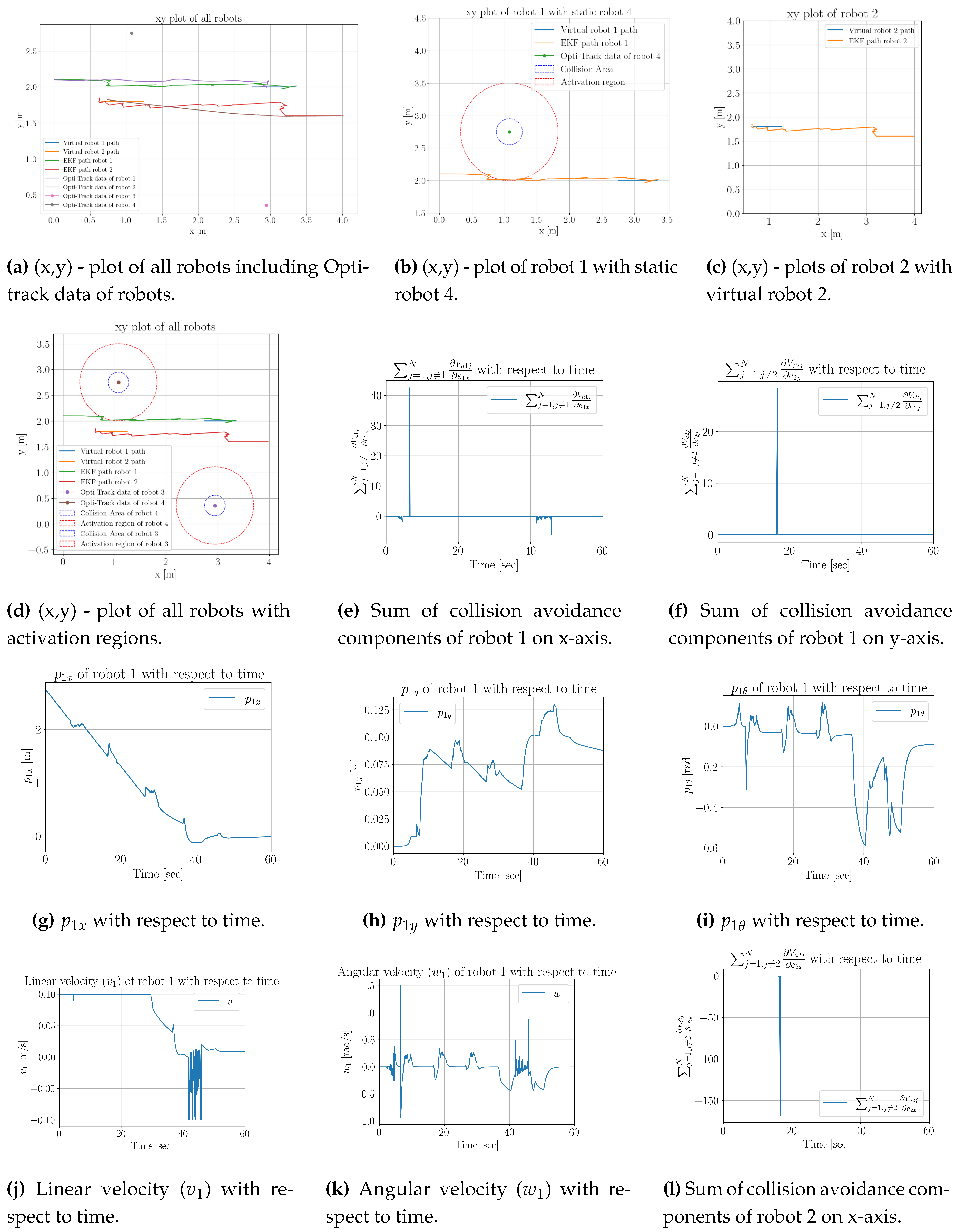
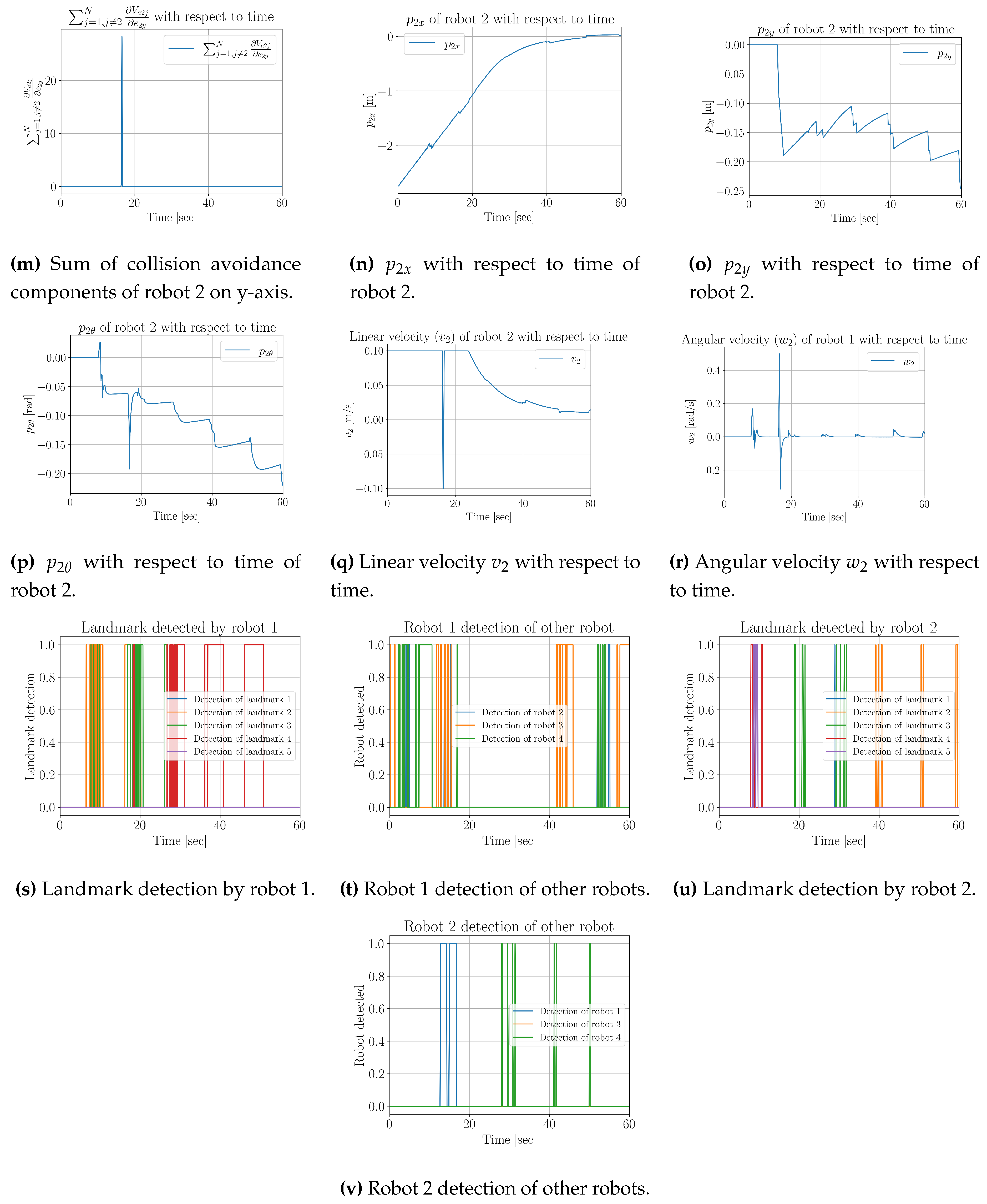

Table 1.
Details of parts used in rotating platform.
| S.No. | Part name | Part details |
|---|---|---|
| 1 | Camera | Intel RealSense sensor D435 |
| 2 | Servo motor | DYNAMIXEL AX-12A |
| 3 | Ball bearing | 6010-2Z |
| 4 | Integrated Circuit (IC) | 74LS241N |
| 5 | Microcontroller | Arduino Mega |
Disclaimer/Publisher’s Note: The statements, opinions and data contained in all publications are solely those of the individual author(s) and contributor(s) and not of MDPI and/or the editor(s). MDPI and/or the editor(s) disclaim responsibility for any injury to people or property resulting from any ideas, methods, instructions or products referred to in the content. |
© 2024 by the authors. Licensee MDPI, Basel, Switzerland. This article is an open access article distributed under the terms and conditions of the Creative Commons Attribution (CC BY) license (http://creativecommons.org/licenses/by/4.0/).
Copyright: This open access article is published under a Creative Commons CC BY 4.0 license, which permit the free download, distribution, and reuse, provided that the author and preprint are cited in any reuse.


