Submitted:
17 December 2024
Posted:
18 December 2024
You are already at the latest version
Abstract
This survey extends and refines the existing definitions of integrity and protection level in localization systems (localization as a broad term, i.e., not limited to GNSS-based localization). In our definition, we study integrity from two aspects: quality and quantity. Unlike existing reviews, this survey examines integrity methods covering various localization techniques and sensors. We classify localization techniques as optimization-based, fusion-based, and SLAM-based. A new classification of integrity methods is introduced, evaluating their applications, effectiveness, and limitations. Comparative tables summarize strengths and gaps across key criteria. The survey presents a general probabilistic model addressing diverse error types in localization systems. Findings reveal a significant research imbalance: 73.3% of surveyed papers focus on GNSS-based methods, while only 26.7% explore non-GNSS approaches like fusion, optimization, or SLAM, with few addressing protection level calculations. Robust modeling is highlighted as a promising integrity method, combining quantification and qualification to address critical gaps. This approach offers a unified framework for improving localization system reliability and safety. This survey provides key insights for developing more robust localization systems, contributing to safer and more efficient autonomous operations.
Keywords:
Integrity
; Protection Level
; Localization
; SLAM
; Fault/Outlier Detection
; Robust Optimization
; Factor Graph
; Fault Detection and Exclusion (FDE)
; Model-based FDE
; Coherence-based FDE)
1. Introduction
Integrity is a crucial evaluation criterion for localization systems, complementing traditional metrics such as accuracy [1,2]. Integrity is a concept widely utilized in the literature to quantify the degree of confidence that can be placed in a localization system. Although this is an informal definition, it highlights the importance of integrity, which is further elaborated in Section 3. For example, achieving high levels of automation as defined by SAE [3] in autonomous driving systems (ADS) requires not only highly accurate localization, but also a guarantee of integrity.
The estimated state of a localization system is affected by different types of errors, as detailed in Section 2.1. To address these errors, methods are needed for both qualifying (see Section 6 and Section 7) and quantifying (see Section 4) their impact on state estimation. The integrity criterion assesses the influence of these errors on the state estimate and provides a quantitative measure of the variation in the estimation error.
The importance of integrity spans various domains. Primarily, safety is paramount. In the United States, motor vehicle crashes result in over 40,000 deaths annually and injuries to over 2 million people [4]. Localization errors can have dire consequences, including incorrect navigation decisions and collisions [5]. In addition, integrity fosters consumer confidence, which is critical for the widespread acceptance of self-driving vehicles [6]. Integrity provides users and stakeholders with a measure of confidence in autonomous systems, enhancing operational efficiency through precise navigation, route planning, and vehicle control. This results in more efficient and seamless road operations. Furthermore, integrity is essential in challenging environments, quantifying system performance and safety in scenarios such as extreme weather or limited vision.
Robotic systems, including autonomous vehicles, consist of sensors, electromechanical components, and algorithms. This survey focuses on methods addressing sensor and algorithm failures, which compromise localization integrity. Due to the diversity of failures, various techniques have been developed to mitigate their effects, as no single approach can handle all faults effectively, see Section 6, Section 7 and Section 8.
Several surveys have reviewed integrity monitoring (IM) methods for GNSS and related systems. For example, [7] is dedicated to GNSS technologies and exposes the so-called "Receiver Autonomous Integrity Monitoring" (RAIM) methods. It classifies integrity techniques, including fault detection, exclusion methods, and protection level computation formulas, as seen in Section 2.2. Similarly, [8] addresses GNSS integrity, focusing on urban transport applications, and highlights challenges and differences between aviation and urban environments while noting open research areas.
The survey [9] reviews IM methods for GNSS, INS, map-assisted, and wireless signal-augmented navigation systems. It covers measurement errors, faults from various data sources, and the integration of sensors with GNSS to improve navigation reliability. The review identifies challenges and highlights the need for advances in fault detection, exclusion, error modeling, and real-time processing. It also explores IM techniques for GNSS/INS with map-matching, discussing map/map-matching errors handling and map constraints.
In contrast, our survey focuses on a wider spectrum of localization systems. We include techniques such as SLAM (Simultaneous Localization and Mapping), fusion algorithms, and optimization-based algorithms. We categorize integrity methods into Fault Detection and Exclusion (FDE), Protection Level (PL), and Robust Modeling. Our detailed analysis covers a wide range of sensors, including LiDAR, cameras, HD maps, INS, and others, offering a broader scope compared to the aforementioned surveys that focus primarily on GNSS. Our review emphasizes integrity in perception-based localization systems and highlights gaps in the literature regarding PL methods for these sensors.
Figure 1 compares GNSS-based integrity methods with other localization systems integrity methods, based on data from [7,8,10,11,12,13,14] for GNSS-based localization method and localization systems with other sensors and technologies that appeared in Section 4, Section 5 and Section 8. The pie chart shows the percentage of research focused on GNSS versus other localization systems. This limited percentage of work on localization systems with different sensors and techniques underscores the need for further exploration in this area. Figure 2 shows the distribution of surveyed papers and reveals a significant gap in PL methods for perception-based localization.
The review aims to:
- Redefine integrity
- Redefine integrity of localization systems
- Redefine protection level
- Introduce robust modeling as a new integrity method
These concepts are redefined because no single, accepted definition exists. The new definitions provide a universal view, helping researchers understand and apply integrity concepts.
Current definitions often overlook important aspects of the integrity of localization systems. Many focus on warnings, trust, or accuracy but miss how integrity should be used as an evaluation criterion. The new definition includes both qualitative and quantitative aspects.
In conclusion, the survey shows the importance of integrity methods in localization systems beyond GNSS. The lack of focus on PL methods in perception-based localization reveals a major research gap. This work offers a clear framework and redefines key concepts to advance the field and create more reliable and robust localization systems.
In brief, the following contributions have been made:
- Comprehensive Overview of Integrity Methods: Provides a thorough review of integrity methods applied to localization systems, covering a wider range of sensors, including LiDAR, cameras, HD maps, INS, and others
- A new Classification Framework: Introduces a new classification framework for integrity methods
- Refined Definitions: Offers updated definitions of integrity and protection levels specific to localization systems, clarifying key concepts and metrics
- An in-depth review and comparative analysis of robust modeling, PL computations, and FDE techniques
- A detailed comparison based on the employed techniques or algorithms, evaluation metrics, data types, sensors, and integrity enhancement.
The subsequent sections of this paper are structured to comprehensively explore the integrity methods for localization systems in autonomous vehicles. Beginning with Section 2, the reader is provided with essential background information explain diverse error types and integrity definitions, including a new definition of integrity. Subsequently, Section 3 systematically introduces a spectrum of integrity methods, offering a potential framework for their categorization. In Section 4, the focus shifts towards addressing various protection level definitions found in the literature, accompanied by the proposal of a new definition. Additionally, in Section 2.3, we review key concepts and parameters used to understand the protection level. Section 6, Section 7 and Section 8 examines techniques aimed at enhancing localization system accuracy, delving into fault detection and exclusion methodologies alongside robust modeling strategies.
2. Background and Foundational Concepts
This section defines the vocabulary used to describe the integrity of localization systems. First of all, this section introduces various error types that localization systems encounter. Then, the different perspectives on the integrity definition appears in the literature are discussed. Finally the section concludes with a proposed integrity definition that encompasses the different dimensions of the definitions found in the literature.
2.1. Errors Types
A localization system can be affected by several types of errors as depicted in Figure 3. These different types of errors jeopardize the integrity of localization systems. The following is a brief overview of each error’s type:
2.1.1. Uncertainty
2.1.2. Bias
2.1.3. Drift
2.1.4. Outlier
Outlier is defined as "an observation which deviates so much from other observations as to arouse suspicions that it was generated by a different mechanism" [16], see Figure 6. This indicates that it is produced by a population different from the one we initially assumed. Consider a point cloud data observation from a LiDAR at time t, , where N is the number of LiDAR beams. This observed point cloud does not contain only the true point cloud data, , but also different types of errors. In order to incorporate all the previous types of errors into a mathematical model, let us consider only one beam, the k-th beam. The previous errors types, except the outlier, can be incorporated in the following mathematical expression:
The PDF for the is given as a . Assuming that the outlier generated with a probability from an unknown PDF given as [16]. Thus, the distribution of an arbitrary LiDAR beam would be :
This model describes all different types of errors that a measured value might experienced.
In localization systems, no one integrity enhancement method can handle all errors types illustrated in Equations (1) and (2).
Figure 7.
Classification of Integrity Methods.
2.2. Integrity Methods in GNSS Systems
Understanding and ensuring integrity in localization systems is critical across various applications. While this paper primarily focuses on perception-based systems, many of the foundational methods for achieving integrity originate from the field of Global Navigation Satellite Systems (GNSS). To provide a brief overview, this section presents key integrity methods used in GNSS systems. This review highlights foundational techniques and concepts. This overview is not exhaustive and does not cover all aspects of GNSS integrity in detail. For a comprehensive review, readers are encouraged to consult the surveys [7,8].
GNSS systems use various integrity methods, mainly categorized into Receiver Autonomous Integrity Monitoring (RAIM) and Protection Level (PL) calculation.
RAIM checks the consistency of multiple satellite signals by computing the position using different subsets of satellites and comparing the results. It requires a minimum of five satellites to detect faults but is typically limited to handling only one faulty satellite at a time.
Different RAIM variants use various measurements, like code or carrier measurements. They also differ in their fault detection capabilities. Advanced RAIM, for instance, can handle multiple faults more effectively compared to traditional RAIM. For a detailed comparison of measurement types and fault detection capabilities in these variants, refer to the surveys [7,8]. In this section, the results from these surveys are summarized and illustrated in Figure 8, with a focus on the RAIM variants.
Protection Level (PL) indicates the potential deviation between the true and estimated positions provided by a GNSS receiver. PL depends on satellite-user geometry and expected pseudorange error. For example, in SBAS (Satellite-Based Augmentation System), PL is calculated as [17]:
where K is an inflation constant and represents the confidence in the estimated position, measured in meters. Accurate PL computation requires knowledge of the distribution of residual position or range errors [18,19,20]. While PL has several formal definitions, discussed in 4, this informal description captures its essence and primary use in GNSS systems.
2.3. Protection Level Related Parameters
To facilitate the understanding of the PL concept, some terms and vocabulary will be introduced. The section will conclude with a proposed definition of PL.
2.3.1. Position Error
Let x represent the estimated pose, and denotes a true pose. The position error, or simply the error, is the difference between the estimated pose and the true pose, . Typically, systems such as RTK-GNSS [21,22] provide an accurate estimation of the true pose. However, the localization system lacks knowledge of the correct path. Position errors are represented by a probability distribution, , which gets altered by numerous types of errors and approximations. In an ideal scenario with a linear system, Gaussian assumptions, and no errors of any types, the final probability distribution function (PDF) would be Gaussian density function, i.e .
2.3.2. Alarm Limit
According to [8], Alarm Limit (AL) "Represents the largest position error allowable for safe operation". Or put it differently it is the maximum value, . Beyond the AL the localization system considered unsafe to rely on.
2.3.3. Integrity Risk (IR)
Or the loss of integrity, it is the probability that the E will exceeds the AL or [8,23,24]. This can be shown mathematically as:
Because the AL changes with time and context, as noted in [25], the PL is used as a more stable alternative. Consequently, in [26,27,28], the Integrity Risk (IR) is defined as:
IR could be intuitively understood as the number of times that the E exceeds the AL, usually per-hour or per-mile. Thus, IR is the probability that a localization system might provide inaccurate poses without alerting the user. It quantifies the likelihood of undetected failures in the system that could result in dangerous or misleading outputs.
2.3.4. Target Integrity Risk (TIR)
TIR Is defined as the accepted level of risk [26,27,28], thus it is an upper bound on the IR.
TIR is the minimum acceptable level of IR that a system must meet to be considered safe and integer within a specific scenario. Where it is specified by industry standards and regulatory agencies, often based on historical data and safety studies. IR is continuously monitored to ensure the system remains within safe limits. Furthermore, IR is measured using system performance data, error models, and operating conditions.
2.3.5. Accuracy
3. Revisiting Integrity: Review, Enhancement, and New Definition
In this section, various definitions of "integrity" as presented in the literature on localization systems are reviewed and analyzed. Each definition’s approach to integrity is examined, where strengths and limitations are highlighted.
Tossaint et al. (2007) [29] define integrity for GNSS-based localization as "the system’s ability to provide warnings to the user when the system is not available for a specific operation." This definition is highly dependent on user application and requirements and limits the measure of integrity to its ability to provide "warnings," which is vague as an indicator. Thus, it requires more specific indicators than just warnings.
Similarly, Ochieng et al. (2003) [30] and Larson (2010) [31] define integrity as "the navigation system’s ability to provide timely and valid warnings to users when the system must not be used for the intended operation or phase of flight". These definitions, while emphasizing warnings, do not address the need for detailed information about issues and potential consequences, allowing them to make informed decisions.
In contrast, AlHage et al. (2021, 2022, 2023) [26,27,28] define integrity as "the ability to estimate error bounds in order to address uncertainty in the localization estimates in real-time." This definition emphasizes the necessity to calculate error bounds that include the real position. Even though the definition does not explicitly mention it, they perform a Fault Detection and Exclusion method, referring to it as internal integrity to enhance the overall system integrity. However, the definition itself is not explicit enough to indicate all these aspects.
Li et al. (2019, 2020) [32,33] describe integrity as "the degree of trust that can be placed on the correctness of the localization solution, and compared it with the used in visual navigation". While this provides a useful measure, it lacks clarity on whether this comparison is specific to vision-based systems or can be generalized to other types of localization systems.
Arjun et al. (2020) [34] define integrity as the measures of overall accuracy and consistency of data sources. However, this definition does not address how faults impact the system. While it focuses on data source consistency, it fails to account for the quantification of fault effects, which is essential for a thorough evaluation of system integrity.
Bader et al. (2017) [35] define integrity as "the absence of improper system alterations". This perspective is quite rigid, treating any fault as a complete loss of integrity. It does not account for the varying impacts of different faults, failing to distinguish between their effects on the system. A clearer approach would involve measuring the impact of faults to better assess system integrity.
Wang et al. (2022) [36] describe integrity as "an important indicator for ensuring the driving safety of vehicles", but do not explain how it relates specifically to localization systems. This definition is too vague and lacks detail on what integrity means in the context of localization.
Quddus et al. (2006) define integrity as "the degree of trust that can be placed in the information provided by the map matching algorithm for each position." This definition focuses exclusively on the map matching algorithm and neglects other aspects of localization systems.
Marchand et al. (2010) [37,38] define integrity as "the measure of trust which can be placed in the correctness of the information supplied by the total system." Similarly, Sriramya (2021) [39] describes it as "the measure of trust that can be placed in the correctness of the estimated position by the navigation system," and Shubh (2023) [40] refers to it as "the measure of trust that can be placed in the accuracy of the information supplied by the navigation system." While these definitions focus on the concepts of trust and correctness, they do not clearly address integrity as an evaluation criterion for the entire localization system. The terms "correctness" and "trust" are used without clear definitions or explanations, leaving a gap in understanding how these concepts relate to a comprehensive assessment of system performance. Thus, these definitions overlook the broader need for evaluating how well the system manages errors and deviations, which are crucial for a full evaluation of its integrity. After reviewing various definitions of integrity, the following definition is proposed to address the gaps in the existing ones:
Definition 3.1 (Integrity).
Integrity refers to the quality of a system being coherent with reality.
Definition 3.2 (Integrity for Localization Systems).
In the context of a localization system, integrity serves as an important evaluation criterion, encompassing both qualifying and quantifying aspects:
- Qualifying aspect: Integrity represents the system’s ability to remain unaltered and effectively handle outliers and errors
- Quantifying aspect: Integrity also involves providing an overbounding measure of how far the system’s outputs can deviate from reality
The reviewed definitions of integrity offer various perspectives but often miss a comprehensive view of localization systems. Many focus narrowly on aspects like warnings, trust, or accuracy, lacking a holistic evaluation criterion. The proposed definition addresses these gaps by combining qualitative and quantitative dimensions. It defines integrity as the system’s alignment with reality, involving robustness, outlier management, and deviation measures.
This framework evaluates localization systems’ robustness and reliability more thoroughly. It includes qualifying methods to ensure system reliability and efficient outlier handling, with Fault Detection and Exclusion (FDE) (Section 6 and Section 7) methods being crucial for error mitigation. Quantifying methods, such as PL Section 4, measure deviations from reality.
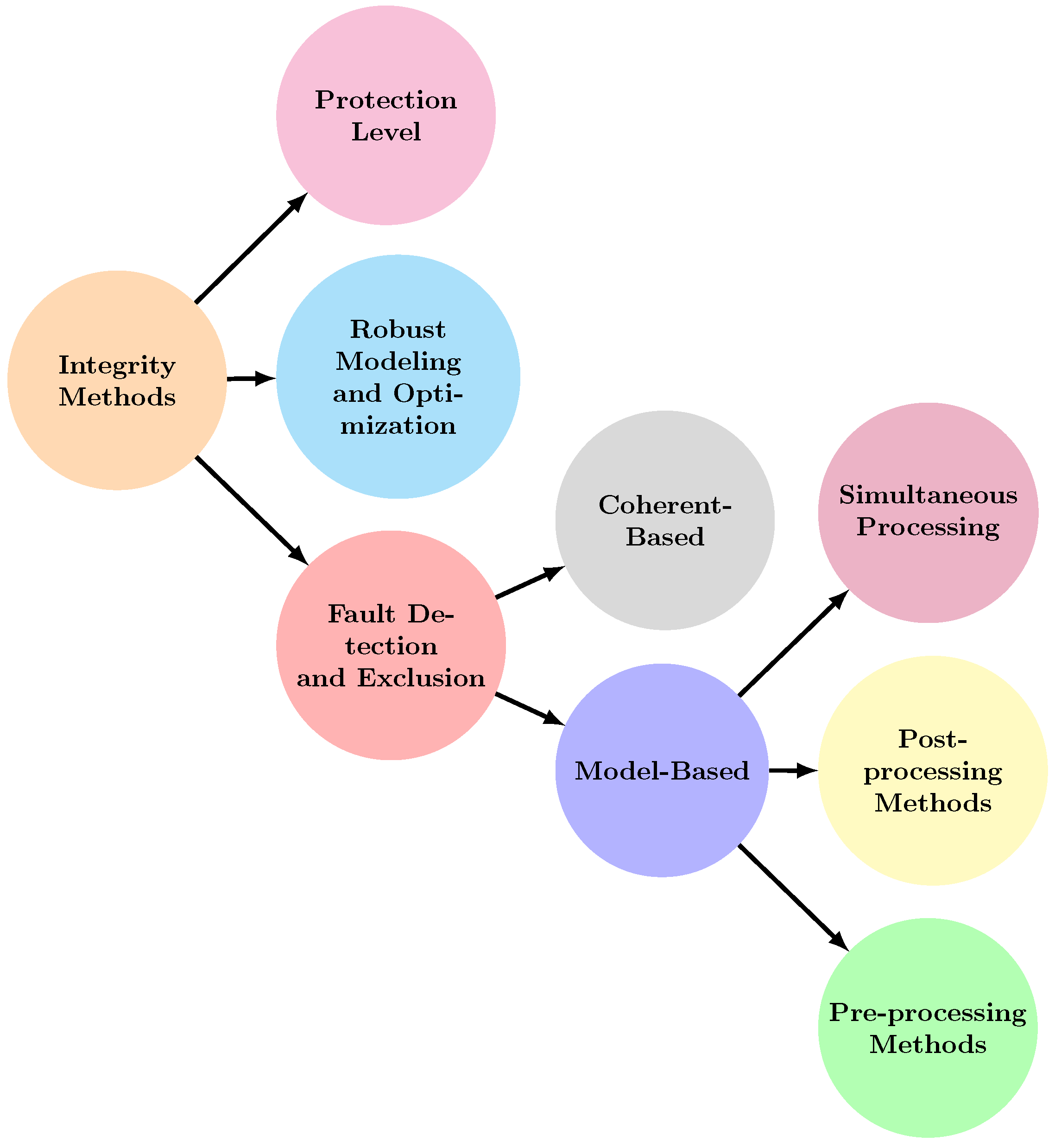
New robust modeling techniques, discussed in Section 8, see Figure 7, are introduced for their ability to handle outliers and provide probabilistic error interpretations. The paper also examines integrity methods across various localization techniques and sensors, ensuring a comprehensive review and defining protection level in line with the paper’s integrity definition.
Quantifying methods measure how far the system’s outputs can deviate from reality, with protection level (PL) providing this overbounding measure. Additionally, this paper introduces robust modeling techniques as new integrity method, see Figure 7 and Section 8. These techniques are chosen for their ability to handle outliers and provide probabilistic interpretations for the error distribution.
4. Protection Level: Current Definitions and New Perspectives
In the following discussion, multiple definitions of PL found in the literature will be outlined. These definitions capture various meanings and applications of PL in the context of integrity for localization systems. Following this review, a proposed definition of PL will be presented to broaden and enhance our understanding of this crucial topic.
Li et al. (2019, 2020) [32,33] describe PL as "the highest translational error results from an outlier that outlier detection systems cannot detect". This definition is limited to translational errors and does not fully address how PL should encompass all types of uncertainties, including those from various sources beyond undetected outliers. Moreover, this definition does not capture the complete error region within which the true position is guaranteed. It also falls short of considering the full scope of errors from all system components and algorithms.
Marchand et al. (2010) [37,38] define PL as "the result of a single undiscovered fault on the positioning error". Similar to the previous definition, this one is confined to undetected faults and does not account for multiple faults or the broader uncertainty inherent in sensor measurements.
The importance of PL as "a statistical bound on position error, E, that guarantees that IR does not exceed TIR" is highlighted by AlHage et al. (2021, 2022, 2023) [26,27,28]. In a similar way, Arjun et al. (2020) [34] and Sriramya (2021) [39] define PL as "an error bound linked to a pre-defined risk". These definitions connect PL to the requirement of a localization system, where TIR is used to check if the system has undetected faults. However, these definitions do not fully address how PL should account for all uncertainties from various system components.A more comprehensive definition of PL should encompass the entire error region, considering all types of uncertainties and limitations of the localization system and its algorithms.
Shubh (2023) [40] defines PL as "the range within which the true position lies with a high degree of confidence," while Wang et al. (2022) [36] describe it as "an upper bound on positioning error". Larson (2010) [31] states PL as "ensuring that position errors remain within allowable boundaries, even with faults". Wang’s use of "upper bound" is too general, while Larson’s focus on error boundaries relates more to system error minimization and handling and does not clearly separate PL from the system’s accuracy.
Overall, current definitions of PL provide useful insights but lack a comprehensive view that includes all uncertainties from various system components and the limitations of the implemented algorithms. To ensure effective use in real-world scenarios, a unified definition of PL is necessary. Therefore, the proposed definition of PL is:
Definition 4.1 (Protection Level).
Protection Level is the real-time estimate or calculation of the error region within which the true position is guaranteed to lie.
By assigning PL to each state estimate, the localization system can effectively adjust to changing environments, sensor conditions, and vehicle dynamics. As a result, system integrity is properly assessed and maintained in real-time.
Figure Figure 9 illustrates how the PL is evaluated at a specific time t. For a given PL, we can compute the probability that the error is below this level based on its probability distribution at time t. Similarly, if we have an AL, we can determine the probability that the error is below the AL. This enables us to calculate the Integrity Risk for the PL, or the AL, .
This is the forward approach: we use a given PL to check if it satisfies the integrity risk criterion. However, the main goal is to determine the PL that meets a specified integrity risk for a given context and period of time. This is done based on the error distribution at that moment of time. Thus, finding the PL that ensure the desired level of integrity risk.
Usually, TIR is used to refine and adjust the PL by tuning its parameters to fit the entire trajectory of the localization system. This is typically done offline, using a learning approach with training and validation data sets, as described in [27]. The goal is to find the parameters that best fit the whole trajectory. In contrast, our focus is on estimating the PL in real-time at each time step based on the current error distribution for a given Integrity Risk.
5. Fault Detection and Exclusion
FDE is crucial for enhancing the integrity of localization system. FDE ensures accurate outputs despite faults or deviations in sensors or algorithms intended behavior. It works by identifying and removing faulty data. "Faults," "failures," and "outliers" often refer to deviations that can negatively impact estimation accuracy. FDE process addresses the qualifying aspect of integrity by making the localization resilient to various error types.
The literature distinguishes between FDE and Fault Detection and Isolation (FDI). FDE focuses on detecting and excluding anomalies to maintain integrity, while FDI aims to identify the specific cause of the problem, which is more relevant in the control engineering and software industries. For localization systems, the key objective is detecting and excluding abnormalities, regardless of their cause. Therefore, this discussion considers all approaches under the category of FDE.
Extensive literature analysis reveals two possible main categories of FDE techniques: model-based and coherence-based approaches. Model-based techniques, Figure 10, utilize mathematical models to predict the system’s behavior, identifying deviations as potential faults. Coherence-based techniques, Figure 11, leverage the consistency among various sensors or measurements of the same quantity, flagging incoherent data points as potential faults.
The following sections explore each category in detail, including methods for computing the protection level. We will use some illustrative figures from the reviewed references. Not all figures will be included; only those that help clarify the process will be selected.
6. Model-Based FDE
In the field of FDE in localization and navigation systems, Model-Based FDE, or MB-FDE, is a vital component, providing reliable solutions through the use of predictive models of system behavior, see Figure 10. These predictive models could be sensor models, system models, or machine learning models like Convolutional Neural Networks (CNN). MB-FDE techniques identifies discrepancies between expected and observed value to detect and exclude faulty data. In the process of this review, a wide range of techniques will be examined, each of which will provide special insights for improving the integrity and PL calculation.
Based on the surveyed paper, MB-FDE is further categorized into three types:
- Post-processing MB-FDE
- Pre-processing MB-FDE
- Simultaneous MB-FDE
- Each of these categories will be explained in the following sections.
6.1. Post-Processing MD-FDE
In the post-processing scheme, detection and exclusion occur after the system state is computed, such as the pose. First, the localization algorithm performs data fusion, Bayesian updates, or optimization. Then, faults or outliers are detected. This means measurements are used as they are, known as the sensor level, and fault detection happens at the system level, like the state or pose. Therefore, detection of faults or outliers happens after the localization processing is complete, see Figure 12. The following provides an in-depth review of post-processing FDE methods found in the literature.
In [26,27,28], an Extended Information Kalman Filter (EIF) is introduced. Banks of EIFs estimate the state using sensors like GNSS, camera, and odometry. Each filter’s output is compared to a main filter that combines, fuse, all outputs. Residuals, calculated as the Mahalanobis distance, used to identify and exclude deviant filters and their sensor data.
PL is calculated by over-bounding the EIF error covariance with a Student’s t-distribution. The degree of freedom for this distribution is adjusted offline during a training phase. However, this method has limitations. It assumes Gaussian noise, which doesn’t accurately represent noise during faults or outliers. The thresholding also depends on this assumption, using Mahalanobis distance compared to a Chi-square distribution. Additionally, the PL calculation is adjusted offline to find the best degree of freedom for the t-distribution for a specific trajectory or scenario.
In [41], a Student t-distribution EIF (t-EIF) is utilized, akin to [26,27,28], but with different residual generation methods. Instead of Mahalanobis distance, it employs Kullback-Leibler Divergence (KLD) between updated and predicted distributions. Residual values adaptively adjust the t-distribution’s degree of freedom, enhancing robustness against outliers. Larger residuals indicate noisy measurements, necessitating thicker tails and lower degrees of freedom, while smaller residuals justify higher degrees of freedom. This adaptation is governed by a negative exponential model, ensuring flexibility and optimization for various measurement conditions. PL calculation depends on degrees of freedom at the prediction and update steps. Errors are adjusted based on the minimum degrees of freedom between these steps. The final PL formula mirrors that of [26,27,28]. Figure 13 shows a general diagram of how the EIF is applied for FDE.
A multirobot system with an FDE step is addressed in [57]. The approach utilizes an EIF-based multisensor fusion system. The Global Kullback-Leibler Divergence (GKLD) between the a priori and a posteriori distributions of the EIF is computed as a residual. This residual, dependent on mean and covariance matrices, is utilized to detect and exclude faults from the fusion process. First, the GKLD is used to detect faults. Next, an EIF bank is designed to exclude faulty observations. The Kullback-Leibler Criterion (KLC) is then used to optimize thresholds in order to achieve the optimal false alarm and detection probability.
In [58], a multirobot system uses EIF for localization. Each robot performs local fault detection based on its updated and predicted states. The Jensen-Shannon divergence (JSD) applied to generate the residuals between distributions. Fault detection thresholds are set using the Youden index from ROC curves. When a fault is detected, JSD is computed for predictions versus corrections from Gyro, MarvelMind, and LiDAR. Residuals are categorized based on their sensitivity to different error types and errors from nearby vehicles. If thresholds are exceeded, residuals are activated using a signature matrix, which helps detect and exclude faults and detects simultaneous errors. Faulty measurements are then removed from the fusion process.
In [52,56], the setup is extended with a new FDE approach and batch covariance intersection informational filter (B-CIIF). Fault detection and exclusion are based on JSD between predicted and updated states from all sensors.
In [52], a decision tree is employed for fault detection, while a random forest classifier is used for fault exclusion. Both methods use JSD residuals and a prior probability of the no-fault hypothesis for training. In contrast, [56] employs two Multi-layer Perceptron (MLP) models. One for fault detection and the other for fault exclusion. The input to the MLPs includes residuals and the prior probability of the no-fault hypothesis. Training data for these machine learning techniques includes various fault categories like gyroscope drift, encoder data accumulation, Marvelmind data bias, and LiDAR errors. However, the limitation of generalizability remains significant. Since the training data is specific to certain scenarios, the models may struggle to detect and address faults in new or unfamiliar environments. This limitation can compromise the overall reliability and integrity of the system when deployed beyond the scope of the training data.
6.2. Pre-Processing MB-FDE
In the preprocessing scheme, fault detection happens at the sensor level. Sensor measurements, such as from LiDAR, cameras, odometry, or GNSS, are first checked for faults or outliers. This means faults are detected and excluded before the data is used in the localization system, whether it involves fusion, Bayesian updates, or optimization, see Figure 14. An in-depth review of pre-processing FDE methods from the literature is presented next.
In GNSS systems, [42] presents a method to reduce residuals between predicted and measured pseudo-range data from satellites. They use a Gaussian Mixture Model (GMM) to handle errors that have multiple modes. Instead of a single linearization point, they use a distribution over this point, managed by a particle filter. Each particle has a vector indicating the weight from each satellite. The particle with the highest total weight is favored, this is called the voting step. This method relies on data from multiple satellites and GNSS receiver correlations over time. If any data is missing, the method’s accuracy declines. Integrity is measured by calculating the likelihood that the estimated pose exceeds the AL region. Figure 15 illustrates the framework adopted in this work.
Integrity is assessed using two metrics: hazardous operation risk and accuracy. Accuracy measures the probability that the estimated pose is outside the AL, while hazardous operation risk examine if the estimated position has at least a probability of containing the true position. An alarm is triggered if either metric exceeds a set threshold, indicating a loss of integrity.
In [32,33], a vision-based localization system enhances ORB-SLAM2 with FDE techniques. It uses a parity space test to detect faults, addressing one fault at a time by comparing expected and observed measurements. Faulty features are removed iteratively until the error hits a threshold. An adaptive residual error calculation accounts for uncertainties. The modular design allows easy integration with existing SLAM techniques. PL considers noise from observations and maximum deviation from undetected faults, calculated as a weighted sum of covariance elements. Improved covariance matrix elements boost computation accuracy by removing inaccurate features or outliers iteratively. A threshold ensures a sufficient number of inliers for SLAM operations; if not met, the location estimate is deemed unsafe.
The technique used for FDE in the image-based navigation system described in [31] is similar to that of GPS RAIM [59,60,61], which is based on performing a parity test for FDE as in [32,33]. PL is calculated based on the maximum slope of the worst-case failure model, similar to concepts discussed in in[43,44]. The author of this work uses a feature-based tracking method for localization.
[37,38] present a method to reduce errors by treating GNSS and odometry data separately. They improve state estimation by using trajectory monitoring and a short-term memory buffer instead of relying on the standard Markovian assumption. Their technique estimates states over a finite horizon and uses sensor residuals and variances to weight GNSS and odometry data.
For fault detection, they calculate sensor residuals, squared errors, and variances. They then weight GNSS and odometry data based on the ratio of each residual to its standard deviation. A Chi-square distribution threshold used for detecting faults. The sensor with the highest weight is prioritized for exclusion.
This approach relies on hyperparameters for its operation. These include the misdetection probability for the protection level calculation and the Chi-square distribution for fault detection. Additionally, the size of the state buffer is a hyperparameter that should be selected based on the environment and scenario.
The technique presented in [36] is customized for FDE in real-time within LiDAR mapping and odometry algorithms. This technique uses a feature-based sensor model to compute the mean and variance of the latest k innovations for the Extended Kalman Filter (EKF) setting. This technique adaptively establishes a threshold for fault detection by using the Chi-square distribution. Thus, the technique can adapt to environmental changes and sensor conditions. Feature-based FDE technique, dynamic thresholding, and real-time noise estimates are combined in this technique to effectively detect and exclude faults in LiDAR odometry and mapping algorithms. The technique lacks a particular formula for estimating the protection level. Its integrity is, however, evaluated by analyzing critical parameters, including error boundaries, missed detection rate, and false alarm rate. Among these parameters, the error bound stands out as a critical signal for integrity assessment, showing the maximum possible pose error.
In [45], each sensor’s output is evaluated using Hotelling’s test, based on expected sensor output and covariance. This allows for accurate fault detection by examining the correlation within the same sensor’s data. By employing the Student t-distribution to overbound measurement noise and measurement innovation sample covariance to inflate it, where measurement noise is adaptively updated. The adaptive updating of the measurement noise covariance is similar to [36]. It takes into account faults and other outliers adaptively. This application uses a UKF localization-based methodology.
The method in [51] uses raw GNSS measurements for FDE, see Figure 16. Vehicle pose is predicted using IMU and Visual Odometry (VO). The error between this prediction and the GPS receiver pose estimate is computed. FDE is implemented using Hierarchical Clustering [62] to detect and exclude faulty satellite signals. Satellites are divided into three clusters based on estimated errors: multi-path, Non-Line of Sight (NLOS), and Line of Sight (LOS) without errors. Initially, each satellite signal is considered a cluster, which is then clustered based on similarity. The three resulting clusters represent the main types of GPS errors. The LOS cluster, presumed to have the most samples, is used to compare expected pseudo-range errors. If this error exceeds a preset threshold, the associated satellite is excluded. The remaining measurements are used to calculate the GPS receiver’s position and velocity. However, selecting and adjusting thresholds lacks standardization, and the method to calculate the threshold in [51] is not specified.
6.3. Simultaneous MB-FDE
In the simultaneous FDE scheme, fault detection is integrated into the real-time processing of sensor data during localization, such as in SLAM-Based localization. As sensor data is collected, it is immediately checked for faults or outliers, often using a weighting or selection method, before being used for localization. This means that the system continuously adjusts how each measurement affects the final output, such as the pose. For example, if a sensor reading is found to be unreliable, it is down-weighted or ignored during the data fusion or optimization steps. Unlike preprocessing or post-processing methods, which handle faults before or after main processing, simultaneous FDE handles faults dynamically as data is processed, see Figure 17. Next, a detailed examination of simultaneous FDE methods in the literature is provided.
A GraphSLAM-based FDE technique is used in [63]. GPS satellites are treated as 3D landmarks by combining GPS data with the vehicle motion model in the GraphSLAM framework, see Figure 18. The algorithm creates a factor graph using pseudo-ranges, a motion model, and broadcast signals. The difference between predicted and measured pseudo-ranges is used to compute residuals, which are weighted in the graph optimization to detect and reject faulty measurements. The sample mean and covariance of these residuals form an empirical Gaussian distribution, used for FDE. New residuals must fall within a region of this distribution to update the mean and covariance. The algorithm iteratively localizes the vehicle and satellites, eliminating faulty measurements, and updates the 3D map through local and global optimization steps.
Building on the previous technique, the authors of [43,44] combine GPS and visual data for integrity monitoring in a GraphSLAM framework. They use GPS pseudoranges, vision pixel intensities, vehicle motion models, and satellite ephemeris to construct a factor graph. Temporal analysis of GPS residuals and spatial analysis of vision data are performed. Superpixel-based intensity segmentation [64,65], using RANSAC [66,67], labels pixels as sky or non-sky to remove vision faults. Residuals for all inputs are included in the graph optimization, with weights to detect faults and/or outliers. GPS FDE relies on temporal correlation, while vision FDE uses spatial correlation. A batch test statistic, the sum of weighted squared residuals, is computed to assess integrity. This statistic follows a Chi-squared distribution, and the protection level is calculated using the non-centrality parameter and the worst-case failure mode slope. This approach is illustrated in Figure 19.
The method in [48] enhances system integrity by estimating both the robot’s position and its reliability. According to [48], reliability is defined as the probability that the estimated pose error falls within an acceptable range. A modified CNN from [68] identifies localization failures by learning from successful and failed localizations. It converts CNN output into a probabilistic distribution using a Beta distribution [69], based on a reliability variable.
The conventional Dynamics Bayesian Network (DBN) model is updated with two new variables, Figure 20: the reliability variable and the CNN output. The DBN uses a Rao-Blackwellized Particle Filter (RBPF) to estimate both reliability and position. Over time, the reliability variable decays if no observations are made. To improve efficiency, [49] introduces a Likelihood-Field Model (LFM) for calculating particle likelihoods. The CNN output uses a sigmoid function to indicate localization success. Positive and negative decisions are modeled with Beta and uniform distributions, respectively, with constants optimized experimentally.
Despite the LFM’s efficiency benefits, it may reduce data representation, affecting failure detection accuracy. The method also faces challenges due to the computational demands of visual data analysis. Domain-specific knowledge and computational resources are needed to determine the constants for optimal performance.
In [50], a more advanced method extends pose and reliability estimation by incorporating observed sensor measurements’ class. This approach includes three latent variables: localization state (successful or failed), measurement class (mapped or unmapped), and vehicle state. A modified LFM is used for observation sensors, and the proposed model integrates information about observed obstacles using conditional class probability [70].
In contrast to the previous methods [48,49], which employed a CNN to make decisions, this strategy uses a basic classifier based on the Mean Absolute Error (MAE) of the residual errors. The residual is the difference between the observed beams and the closest obstacle in the occupancy grid map. The final decision is computed using a threshold. This method includes both global localization using the free-space feature proposed in [71] and local pose tracking using the MCL presented in [55]. As such, it can perform relocalization due to pose tracking failure. The method in [72] is used to fuse the local and global localization approaches via importance Importance Sampling (IS).
In [40,46], a method is proposed to enhance camera-based localization in GNSS-limited areas by improving PL calculations. The approach leverages CNNs and 3D point cloud maps from LiDAR to estimate location error distributions, capturing both epistemic and aleatoric uncertainties [73,74].
The CNN has two components, Figure 21: one estimates position error, and the other calculates covariance matrix parameters. It uses CMRNet [75] with correlation layers [76] for error estimation, and a model similar to [77] for covariance.
To handle CNN fragility, the method applies outlier weighting using robust Z-scores. A GMM is built from weighted error samples to represent position errors and calculate PL from the GMM’s cumulative distribution function.
However, the method’s effectiveness is limited by the need for large, high-quality training datasets, which can be labor-intensive and affect accuracy due to variability in input data and dataset quality.
6.4. Model-Based FDE Methods: Summary and Insights
MB-FDE algorithms are promising for fault handling in localization systems but face scalability and reliability challenges. The reliance on correct sensor data, as well as the assumption of specific noise distributions, may limit their application in real-world scenarios with a wide range of environments and sensors. Practical implementation is further complicated by the computational complexity of analyzing several failure hypotheses and the combinatorial explosion in the number of measurements. Furthermore, the efficiency of these strategies is strongly reliant on the proper modeling of temporal and spatial correlations, which is not always simple or precise. Overall, while these FDE techniques are significant advances in maintaining the integrity of localization systems, more research is needed to overcome their shortcomings and increase their robustness in a variety of operating environments.
7. Coherence-Based Techniques
These techniques use the consistency of data from various sensors or localization systems to perform FDE. Fundamentally, coherence-based FDE, or CB-FDE, techniques take advantage of the idea that, in typical operational environments, several estimates of the same quantity should show coherence or agreement. These estimates can be acquired by different sensors, systems, or algorithms. Usually, the coherency check is carried out by weighing the estimates from each source and accepting the set of estimates that satisfy a threshold test. Alternatively, a test between each pair of estimate sources can be performed to check for inconsistencies. This in-depth analysis will examine a wide range of algorithms and approaches, each providing unique perspectives and techniques for identifying and eliminating faults.
An innovative approach for detecting localization failures is introduced by [78]. It examines the coherency between sensor readings and the map by analyzing latent variables. The model uses Markov Random Fields (MRF) [79,80] with fully connected latent variables [81] to find misalignments. These latent variables can be aligned, misaligned, or unknown, based on residual errors between measurements and the map.
The method integrates with the localization module and uses the 3D Normal Distribution Transform (3D-NDT) scan-matching technique [82,83]. It estimates the posterior distribution of latent variables from residual errors and applies a probabilistic likelihood model. The model includes a hyperparameter and selection bias. Failure probability is approximated using sample-based methods, though the precision of this approximation is not verified. The model’s multimodality, due to latent variables, may not capture all possible outcomes. The technique from [34] integrates data from LiDAR, cameras, and maps into a unified model, as shown in Figure 22. It maintains data consistency through redundancy and weighting. The method aligns sensor data with map data using GPS positions. A Feature Grid (FG) is used to label physical areas and assign weights based on distance. This FG model overcomes limitations of traditional geometrical models by representing different features with labels and evaluating coherence between feature grids, see Figure 23.
The particle filter from [84] is adapted for map matching, creating a uniform integrity testing framework. This approach avoids specific thresholds and does not rely on particular error noise models. The PL, including the Horizontal Protection Level (HPL), is calculated using the variances of particle distributions from sensor combinations, focusing on average standard deviation.
The technique in [85] uses multiple localization systems to detect and recover from faults. It combines an EKF with a Cumulative Sum (CUSUM) test [86] to detect faults and estimate the time when they occur. The EKF tracks outputs from various systems, comparing them to find deviations. The CUSUM test helps reduce false alarms by monitoring these deviations. When a fault is detected, the system uses stored sensor data for position estimation based on the fault time. This method does not need a specific fault model, simplifying implementation. However, it lacks the ability to exclude faults and relies on assumptions about system consistency, which may lead to false alarms or missed detections.
The approach in [87] uses EKF for sensor fusion in SLAM. It integrates multiple sensors, including MarvelMind for localization, gyroscopes, encoders, and LiDAR, with two EKFs: EKF-SLAM1 processes encoder and LiDAR data, while EKF-SLAM2 handles encoder and gyro data. Faults are detected by comparing Euclidean distances between EKF positions and MarvelMind data against a threshold. A large residual indicates a fault if it exceeds this threshold. Faults are identified by specific residual subsets, simplifying fault exclusion in sensors like gyroscopes and indoor GPS. When both encoder and laser rangefinder fail, angular velocities are compared to find the faulty sensor. This method requires a global position estimate from MarvelMind to function correctly.
Research by [35] introduces a method for enhancing fault tolerance in multisensor data fusion systems. It uses two separate data fusion systems to ensure that only one fault occurs at a time. When a fault is detected, the system compares outputs from duplicated sensors and data fusion blocks. It measures the Euclidean distance between two EKF outputs and checks it against a preset threshold. If the distance is too high, it indicates a fault. The process involves two steps: comparing residuals and sensor outputs. Hardware faults are identified by comparing sensor outputs, while faulty localization systems are detected through residual comparison. The system recovers by using error-free localization values. However, setting detection thresholds can be expensive and context-specific.
In [88], a combined approach of model-based and hardware redundancy addresses drift-like failures in wheels and sensors. Model-based redundancy uses a mathematical model to mimic component behavior. The technique employs a bank of EKF and three gyroscopes, each assigned to specific faults, producing distinct residual signatures for fault detection. Residuals are used to identify faults in wheels, encoders, and gyroscopes. A fault is flagged if the residual exceeds three times its standard deviation for a set number of times. Simulations demonstrate the technique’s effectiveness in detecting sensor and actuator failures. However, the initial thresholds for fault detection, based on the three-sigma rule, do not adapt well to varying conditions. This can lead to false alarms or missed detections, affecting the system’s accuracy in dynamic environments.
In [89], a process model predicts the initial pose by integrating data from stereoscopic systems, LiDAR, and GPS for vehicle localization. GPS provides the absolute position, while stereoscopic systems and LiDAR estimate ego-motion. The method uses the extended Normalized Innovation Squared (NIS) test to ensure sensor coherence before data fusion. Faulty sensor observations are removed before integration. LiDAR accuracy is improved with Iterative Closest Point (ICP) and outlier rejection. Sensor coherence is checked using the extended NIS test. An Unscented Information Filter (UIF) integrates data from multiple sensors, minimizing error accumulation. Parity relations [90], calculated with Mahalanobis distance, help detect faults.
However, this method assumes only one fault occurs at a time, which may not reflect real-world scenarios. It also assumes Gaussian sensor readings, which may not be accurate in complex situations. Moreover, the Gaussian assumption may not handle noise or outliers efficiently, potentially leading to incorrect fault detection. Accurate sensor modeling and calibration are challenging, and computational costs increase with more sensors.
In [91,92], the maximum consensus algorithm localizes the vehicle. [91] uses LiDAR data, while [92] converts 3D LiDAR point clouds into 2D images. An approximate pose is aligned with a georeferenced map point cloud. The search for the vehicle’s position is limited to a predefined range, ensuring the true position is within it. Candidate positions are discretized, and a consensus set is created for each cell by counting matches between map points and sensor scan points, using a distance threshold and classical ICP cost function [93,94,95,96].
An exhaustive search finds the global optimum by identifying the transformation with the highest consensus. Despite the exponential cost with more dimensions, the search becomes constant with fixed dimensions. The algorithm covers the entire objective function distribution, and parallel processing is facilitated by simple count operations. Real-time applications benefit from discrete optimization techniques like branch-and-bound [97,98], which speed up computations.
However, [91,92] have limitations due to its simplistic counting approach. It does not fully account for the importance of correspondences in vehicle pose estimation, especially in urban environments where most matches are from the ground and facades. [92] introduces a new objective function that uses normal vectors for point-to-surface matching, improving constraints, especially longitudinally. Errors are measured using the covariance matrix of position parameters, with a smaller trace1 indicating fewer errors. Helmert’s point error, the inverse of the matrix trace, scores solution quality, guiding localization. The algorithm uses a physical beam model [55] to create a probability grid from LiDAR data, defining the PL from grid cells with a probability . A significant drawback is the grid-based search constraint, which limits precision to the resolution of the search space. Handling irregular point cloud distributions remains challenging, even with point-to-surface mapping.
7.1. Coherence-Based FDE Methods: Summary and Insights
CB-FDE techniques have a number of shortcomings. As the number of sources rises, scalability problems occur, and comparisons grow quadratically. For example, 10 sources require 45 comparisons, whereas 20 sources demand 190. This leads to increased computational complexity, making real-time problem detection difficult owing to processing delays. Additionally, these techniques rely on redundancy, which is less successful in systems with fewer sources because it requires multiple sources to provide the same value. Furthermore, as CB-FDE performs best with errors that consistently affect all sources, it is less effective with irregular error patterns.
Table 4 summarizes all MB-FDE methods and compares them using various criteria.
8. Robust Modeling and Optimization
FDE methods primarily focus on qualifying system integrity by detecting and managing faults and outliers. Qualification in this context means determining whether the system is functioning correctly by identifying when and where things go wrong. However, FDE methods often fall short in the quantification of integrity, which involves measuring the extent or impact of these faults. Without quantification, it is difficult to assess how errors affect the overall system performance. To address this gap, additional techniques, such as PL, are required to provide a numerical measure of system integrity.
Robust modeling and optimization techniques address both qualification and quantification. These methods do not depend on specific fault models; instead, they use general approaches to handle a wide variety of faults and noise. This allows for both a thorough assessment of whether the system is performing correctly (qualification) and a measurement of how well it is performing (quantification). By providing probabilistic interpretations of error distributions, robust methods give a more complete picture of system integrity.
In localization tasks, the common assumption that errors follow a Gaussian distribution often fails. This is not only because of linear approximations in algorithms like factor graphs and Bayesian methods, but also due to other factors such as the presence of unknown outlier distributions, see Section 2.1.4.
These outliers can arise from various front-end [100] processes involved in building the factor graph, such as:
- Loop Closure Detection [104]: In SLAM-based localization, incorrect identification of loop closures can distort the graph and lead to substantial errors
- Mapping Errors [103,108,109,110]: Outliers can also arise due to inaccuracies in the map itself, which may result from errors accumulated during the map generation process. These mapping errors can propagate through the system, leading to further mismatches during map matching and adding additional outliers.
These front-end issues, if not properly handled, can weaken both the qualification and quantification of system integrity.
Robust modeling techniques are particularly valuable in these scenarios because they can manage diverse sources of error without needing detailed models of every possible fault. Unlike traditional methods, robust algorithms dynamically adapt to uncertainties in real-time, which is crucial in complex, changing environments. These algorithms effectively mitigate the impact of various uncertainties, making them essential for both qualifying and quantifying system performance.
In localization, robust modeling is often applied using a factor graph model[111,112,113], as shown in Figure 24. In this model, a graph representation is adopted, where nodes correspond to different states or poses, and edges represent constraints between them. These constraints can come from various sources, such as:
- Odometry: Using methods like ICP from image sequences or LiDAR scans, or motion models from IMU data
- GPS: Providing positional constraints based on satellite data
- Map Matching: Aligning sensor data with a known map
- Landmarks Observations: Constraints from observing known landmarks
- Calibration Parameters: Constraints related to sensor calibration
These constraints generate residuals, and the sum of these residuals represents the total energy or loss of the graph. The goal of optimization is to minimize this loss, thereby refining the graph’s configuration to best fit the sensory information. Factor graph optimization can be performed either online, as data is received, or offline, using a batch of data.
By addressing both the qualification and quantification of errors, robust modeling ensures that the system not only identifies faults but also accurately measures their impact, leading to a resilient and precise localization system. This approach is particularly crucial in environments where the quality of the sensor’s data can significantly influence the overall performance.
This section reviews the primary algorithms and techniques used to create robust localization algorithms.
8.1. Analysis of Robust Modeling and Optimization Techniques
Current localization methods often use least squares optimization but face challenges when dealing with outliers like data association errors and false positive loop closures.
To address these issues, [114] introduced a solution that improves the back-end optimization process. Instead of keeping the factor graph structure or topology fixed, this method allows the graph topology to change dynamically during optimization. This flexibility helps the system detect and reject outliers in real-time, making SLAM more robust. The method uses switch variables, see Figure 25, for each potential outlier constraint or edge. These variables help the system decide which constraints to include or exclude based on their accuracy. Essentially, switch constraints (SC) act as adjustable weights for each factor in the factor graph. These weights are optimized along the map for SLAM [114] and the pose for GNSS-based localization [115,116].
This approach is similar FDE because it automatically identifies and removes erroneous data associations or pseudo measurements, ensuring the system uses only reliable data [114,115,116]. However, this approach introduced extra switch variables for each potential outlier, which increased both the computational cost and complexity of each iteration. As a result, the system could become less efficient and slower to converge.
In contrast, Dynamic Covariance Scaling (DCS) [118,119,120,121] offers a more efficient method for managing outliers in SLAM without adding extra computational load. DCS adjusts the covariance of constraints based on their error terms, changing the information matrix without needing additional variables. This makes the optimization process more efficient and speeds up convergence. The scaling function in DCS is determined analytically and is related to weight functions in M-estimation [122], which reduces the number of parameters to estimate compared to the SC approach, since DCS does not require iterative optimization of the scaling function.
The earlier methods using SC and DCS had challenges with tuning the scaling function based on error, and also required manual adjustment of parameters [123]. The method in [124] addresses this issue with self-tuning M-estimators. This approach directly adjusts the parameters of M-estimator cost functions, which simplifies the tuning process.
The self-tuning M-estimators method connects M-estimators with elliptical probability distributions, as introduced in [124]. This means that M-estimators can be chosen based on the assumption that errors follow an elliptical distribution. The algorithm then automatically adjusts the parameters of the M-estimators during optimization, selecting the best one based on the data’s likelihood.
A broader approach to robust cost functions is introduced in [125]. This method improves algorithm performance for tasks like clustering and registration by treating robustness as a continuous parameter. The robust loss function in this framework can handle a wide range of probability distributions, including normal and Cauchy distributions, by using the negative log of a univariate density. By incorporating robustness as a latent variable in a probabilistic framework, this approach automatically determines the appropriate level of robustness during optimization, which eliminates the need for manual tuning and provides a more flexible solution.
Building on this, [126] presents a method that dynamically adjusts robust kernels based on the residual distribution during optimization. This dynamic tuning improves performance compared to static kernels and previous methods. The key difference from [125] is that the new method covers a wider range of probability distributions by extending the robust parameter’s range. The shape of the robust kernel is controlled by a hyperparameter that adjusts in real-time, enhancing both performance and robustness. Figure 26 represents various robust kernels and the switching between them during optimization. The switching between these kernels during optimization occurs due to the fact that robustness is modeled by an optimizable latent variable.
In contrast, [127] introduces a probabilistic approach to improve convergence. This method fits the error distribution of a sensor fusion problem using a multimodal GMM. In real-time applications like GNSS localization, the adaptive mixing method adjusts to the actual error distribution and reduces reliance on prior knowledge. This approach effectively handles non-Gaussian measurements by accurately accounting for their true distribution during estimation. In sensor fusion, where asymmetric or multimodal distributions are common, this method provides a probabilistically accurate solution. It uses a factor graph-based sensor fusion approach and optimizes the GMM adaptation with the Expectation Maximization (EM) algorithm [128,129].
In [40,130], a robust multisensor state estimation method combines a Particle Filter (PF) with a robust Extended Kalman Filter (R-EKF) using RBPF. It replaces the Gaussian likelihood with robust cost functions like Huber or Tukey biweight loss [122] to better handle non-Gaussian errors and outliers unlike standard EKF methods [131,132]. The approach uses PF for linearization points and R-EKF for state estimation, integrating estimates across points with resampling [133]. Position error bounds are estimated using a GMM and Monte Carlo integration [55], addressing orientation uncertainty and providing robust probabilistic bounds. Limitations include sensitivity to initial parameters, potential convergence to local optima, and added complexity in tuning and balancing loss terms, which can introduce biases or errors.
8.2. Robust Modeling and Optimization: Summary and Insights
In conclusion, this section underscores the importance of both FDE techniques and robust modeling approaches for enhancing the integrity of localization systems. FDE qualifies system integrity by managing faults and deviations but doesn’t measure their impact on performance. Robust modeling qualifies and quantifies integrity by handling errors and providing probabilistic error bounds. Specifically, robust modeling offers two key features: it associates a probabilistic distribution over the error and dynamically accounts for variations in system uncertainty as described in [125,126]. Thus, to fully address the integrity of localization system, integrating FDE or robust modeling with PL is essential.
Lastly, while PL quantifies integrity, the evaluation of integrity varies across applications. This typically involves computing the Integrity Risk (IR) and comparing it with the Total Integrity Risk (TIR) to determine the likelihood of the true position exceeding the provided PL, as described in Section 4.
Table 5 summarizes all the robust methods and compares them using various criteria.
9. Conclusion
In conclusion, this survey paper presents several significant contributions to the field of integrity methods in localization systems. It identifies a crucial gap in the research on integrity methods for non-GNSS-based systems, highlighting the need for more efforts in this area.
While of surveyed literature focuses on GNSS-based systems, only covers non-GNSS systems that use various sensors and approaches, such as cameras, LiDAR, fusion, optimization, or SLAM. Furthermore, among these, only a small fraction specifically explores protection level calculations.
This paper introduces a unified definition of integrity that encompasses both qualitative and quantitative aspects, cf. Section 3. The new definition integrates robustness, outlier management, and deviation measures, providing a holistic evaluation of localization systems. The proposed framework improves upon existing definitions by offering a comprehensive view that includes the system’s alignment with reality and detailed error handling.
The survey reviews and refines the definitions of Protection Level (PL), cf. Section 4. It points out that current definitions do not account for all uncertainties and limitations from system components and algorithms. The new definition of PL provided here addresses these gaps by requiring a real-time estimate of PL. This definition facilitates effective adjustment to changing environments and sensor conditions, ensuring real-time system integrity assessment.
The survey provides a detailed review of Fault Detection and Exclusion (FDE) methods. The FDE techniques are categorized into model-based and coherence-based approaches, examining their applications, effectiveness, and limitations. Model-based FDE methods are further divided into post-processing, pre-processing, and simultaneous-processing categories. While these methods are promising for fault handling, they face challenges related to scalability, reliability, computational complexity, model selection and accurate modeling. Coherence-based FDE techniques also encounter issues with scalability and effectiveness, particularly with irregular error patterns.
Moreover, the paper introduces robust modeling and optimization as essential methods for integrity. Unlike traditional FDE methods that focus primarily on qualification, robust modeling addresses both qualification and quantification. It provides probabilistic error bounds and adapts to variations in system performance, offering a more comprehensive view of integrity. This approach allows for a thorough assessment of system performance and measurement of how well it is functioning.
Finally, the survey includes comparative tables that summarize and evaluate various integrity methods, highlighting their strengths and limitations. This comparative analysis provides a clearer understanding of how different methods can be applied across various localization systems.
Overall, this paper offers a valuable reference for researchers and practitioners, presenting a detailed review of integrity methods, new definitions, and a comprehensive classification framework. It sets a foundation for future research and development, aiming to enhance the safety and efficiency of localization technologies by addressing key gaps and offering a more complete understanding of integrity and protection levels.
Author Contributions
Conceptualization, Maharmeh, Alsayed, and Nashashibi; formal analysis, Maharmeh; visualization, Maharmeh, Alsayed, and Nashashibi; writing—original draft preparation, Maharmeh and Alsayed; writing—review and editing, Maharmeh; supervision, Nashashibi. All authors have read and agreed to the published version of the manuscript.
Funding
This research received no external funding
Conflicts of Interest
The authors declare no conflicts of interest.
References
- Allen, M.; Baydere, S.; Gaura, E.; Kucuk, G. Evaluation of localization algorithms. In Localization Algorithms and Strategies for Wireless Sensor Networks: Monitoring and Surveillance Techniques for Target Tracking; IGI Global, 2009; pp. 348–379.
- Shan, X.; Cabani, A.; Chafouk, H. A Survey of Vehicle Localization: Performance Analysis and Challenges. IEEE Access 2023. [CrossRef]
- SAE, J. 3016-2018, taxonomy and definitions for terms related to driving automation systems for on-road motor vehicles. Society of Automobile Engineers, sae. org 2018.
- Wansley, M.T. Regulating Driving Automation Safety. Emory Law Journal 2024, 73, 505.
- Patel, R.H.; Härri, J.; Bonnet, C. Impact of localization errors on automated vehicle control strategies. 2017 IEEE Vehicular Networking Conference (VNC). IEEE, 2017, pp. 61–68.
- Bosch, N.; Baumann, V. Trust in Autonomous Cars. I: Seminar Social Media and Digital Privacy, 2019.
- Zabalegui, P.; De Miguel, G.; Pérez, A.; Mendizabal, J.; Goya, J.; Adin, I. A review of the evolution of the integrity methods applied in GNSS. IEEE Access 2020, 8, 45813–45824.
- Zhu, N.; Marais, J.; Bétaille, D.; Berbineau, M. GNSS position integrity in urban environments: A review of literature. IEEE Transactions on Intelligent Transportation Systems 2018, 19, 2762–2778. [CrossRef]
- Jing, H.; Gao, Y.; Shahbeigi, S.; Dianati, M. Integrity monitoring of GNSS/INS based positioning systems for autonomous vehicles: State-of-the-art and open challenges. IEEE Transactions on Intelligent Transportation Systems 2022, 23, 14166–14187. [CrossRef]
- de Oliveira, F.A.C.; Torres, F.S.; García-Ortiz, A. Recent advances in sensor integrity monitoring methods—A review. IEEE Sensors Journal 2022, 22, 10256–10279.
- Hassan, T.; El-Mowafy, A.; Wang, K. A review of system integration and current integrity monitoring methods for positioning in intelligent transport systems. IET Intelligent Transport Systems 2021, 15, 43–60. [CrossRef]
- Hewitson, S.; Wang, J. GNSS receiver autonomous integrity monitoring (RAIM) performance analysis. Gps Solutions 2006, 10, 155–170. [CrossRef]
- Angrisano, A.; Gaglione, S.; Gioia, C. RAIM algorithms for aided GNSS in urban scenario. 2012 Ubiquitous Positioning, Indoor Navigation, and Location Based Service (UPINLBS). IEEE, 2012, pp. 1–9.
- Bhattacharyya, S.; Gebre-Egziabher, D. Kalman filter–based RAIM for GNSS receivers. IEEE Transactions on Aerospace and Electronic Systems 2015, 51, 2444–2459.
- Hofmann, D. 48: Common Sources of Errors in Measurement Systems 2005.
- Hawkins, D.M. Identification of outliers; Vol. 11, Springer, 1980.
- SC, R. Minimum Operational Performance Standards for Global Positioning System/Wide Area Augmentation System Airborne Equipment. RTCA DO-229 1996.
- Brown, R.G. GPS RAIM: Calculation of thresholds and protection radius using chi-square methods; A geometric approach; Radio Technical Commission for Aeronautics, 1994.
- Walter, T.; Enge, P. Weighted RAIM for precision approach. Proceedings of Ion GPS. Institute of Navigation, 1995, Vol. 8, pp. 1995–2004.
- Young, R.S.; McGraw, G.A.; Driscoll, B.T. Investigation and comparison of horizontal protection level and horizontal uncertainty level in FDE algorithms. Proceedings of the 9th International Technical Meeting of the Satellite Division of The Institute of Navigation (ION GPS 1996), 1996, pp. 1607–1614.
- Fredeluces, E.; Ozeki, T.; Kubo, N.; El-Mowafy, A. Modified RTK-GNSS for Challenging Environments. Sensors 2024, 24, 2712. [CrossRef]
- Lee, S.J.; Kim, B.; Yang, D.W.; Kim, J.; Parkinson, T.; Billingham, J.; Park, C.; Yoon, J.; Lee, D.Y. A compact RTK-GNSS device for high-precision localization of outdoor mobile robots. Journal of Field Robotics 2024.
- EGA. Report on the performance and level of integrity for safety and liability critical multi-applications 2015.
- Mink, M. Performance of receiver autonomous integrity monitoring (RAIM) for maritime operations. PhD thesis, Dissertation, Karlsruhe, Karlsruher Institut für Technologie (KIT), 2016, 2016.
- Bonnifait, P. Localization Integrity for Intelligent Vehicles: How and for what? 33rd IEEE Intelligent Vehicles Symposium (IV 2022), 2022.
- Hage, J.A.; Xu, P.; Bonnifait, P.; Hage, J.A.; Xu, P.; Bonnifait, P.; Integrity, H.; With, L.; Hage, J.A.; Xu, P.; Bonnifait, P. High Integrity Localization With Multi-Lane Camera Measurements To cite this version : HAL Id : hal-02180609 High Integrity Localization With Multi-Lane Camera Measurements 2021.
- Hage, J.A.; Xu, P.; Bonnifait, P.; Ibanez-Guzman, J. Localization Integrity for Intelligent Vehicles Through Fault Detection and Position Error Characterization. IEEE Transactions on Intelligent Transportation Systems 2022, 23, 2978–2990. doi:10.1109/TITS.2020.3027433. [CrossRef]
- Hage, J.A.; Bonnifait, P. High Integrity Localization of Intelligent Vehicles with Student ’ s t Filtering and Fault Exclusion 2023. pp. 24–28. doi:10.1109/ITSC57777.2023.10422598. [CrossRef]
- Tossaint, M.; Samson, J.; Toran, F.; Ventura-Traveset, J.; Hernández-Pajares, M.; Juan, J.; Sanz, J.; Ramos-Bosch, P. The Stanford–ESA integrity diagram: A new tool for the user domain SBAS integrity assessment. Navigation 2007, 54, 153–162. [CrossRef]
- Ochieng, W.Y.; Sauer, K.; Walsh, D.; Brodin, G.; Griffin, S.; Denney, M. GPS integrity and potential impact on aviation safety. The journal of navigation 2003, 56, 51–65. [CrossRef]
- Larson, C.D. An integrity framework for image-based navigation systems 2010.
- Li, C.; Waslander, S.L. Visual Measurement Integrity Monitoring for UAV Localization. 2019 IEEE International Symposium on Safety, Security, and Rescue Robotics, SSRR 2019 2019, pp. 22–29. https://doi.org/10.1109/SSRR.2019.8848975.
- Li, C. Two Methods for Robust Robotics Perception: Visual Measurement Integrity Monitoring for Localization and Confidence Guided Stereo 3D Object Detection 2020.
- Balakrishnan, A.; Florez, S.R.; Reynaud, R. Integrity monitoring of multimodal perception system for vehicle localization. Sensors (Switzerland) 2020, 20, 1–16. doi:10.3390/s20164654. [CrossRef]
- Bader, K.; Lussier, B.; Schön, W. A fault tolerant architecture for data fusion: A real application of Kalman filters for mobile robot localization. Robotics and Autonomous Systems 2017, 88, 11–23.
- Wang, Z.; Li, B.; Dan, Z.; Wang, H.; Fang, K. 3D LiDAR Aided GNSS/INS Integration Fault Detection, Localization and Integrity Assessment in Urban Canyons. Remote Sensing 2022, 14. doi:10.3390/rs14184641. [CrossRef]
- Le Marchand, O.; Bonnifait, P.; Ibañez-Guzmán, J.; Bétaille, D. Automotive localization integrity using proprioceptive and pseudo-ranges measurements. Accurate Localization for Land Transportation, 2009, Vol. 125, pp. 7–12.
- Le Marchand, O.; Bonnifait, P.; Ibañez-Guzmán, J.; Bétaille, D. Vehicle localization integrity based on trajectory monitoring. 2009 IEEE/RSJ International Conference on Intelligent Robots and Systems. IEEE, 2009, pp. 3453–3458.
- Dissertation, S.B. RISK-RESILIENT GPS-BASED POSITIONING, NAVIGATION, AND TIMING USING SENSOR FUSION AND MULTI-AGENT PLATFORMS.
- Gupta, S. High-Integrity Urban Localization: Bringing Safety in Aviation to Autonomous Driving. PhD thesis, Stanford University, 2023.
- Al Hage, J.; Salvatico, N.; Bonnifait, P. High Integrity Localization of Intelligent Vehicles with Student’s t Filtering and Fault Exclusion. 2023 IEEE 26th International Conference on Intelligent Transportation Systems (ITSC). IEEE, 2023, pp. 1341–1348.
- Gupta, S.; Gao, G.X. Reliable GNSS Localization Against Multiple Faults Using a Particle Filter Framework. arXiv preprint arXiv:2101.06380 2021.
- Bhamidipati, S.; Gao, G.X. Integrity monitoring of Graph-SLAM using GPS and fish-eye camera. NAVIGATION: Journal of the Institute of Navigation 2020, 67, 583–600, doi:10.1002/navi.381. [CrossRef]
- Bhamidipati, S.; Gao, G.X. SLAM-based integrity monitoring using GPS and fish-eye camera. Proceedings of the 32nd International Technical Meeting of the Satellite Division of The Institute of Navigation (ION GNSS+ 2019), 2019, pp. 4116–4129.
- Mori, D.; Sugiura, H.; Hattori, Y. Adaptive sensor fault detection and isolation using unscented kalman filter for vehicle positioning. 2019 IEEE Intelligent Transportation Systems Conference (ITSC). IEEE, 2019, pp. 1298–1304.
- Gupta, S.; Gao, G. Data-driven protection levels for camera and 3D map-based safe urban localization. Navigation 2021, 68, 643–660.
- Geiger, A.; Lenz, P.; Urtasun, R. Are we ready for Autonomous Driving? The KITTI Vision Benchmark Suite. Conference on Computer Vision and Pattern Recognition (CVPR), 2012. [CrossRef]
- Akai, N.; Morales, L.Y.; Murase, H. Simultaneous pose and reliability estimation using convolutional neural network and Rao–Blackwellized particle filter. Advanced Robotics 2018, 32, 930–944. https://doi.org/10.1080/01691864.2018.1509726. [CrossRef]
- Akail, N.; Moralesl, L.Y.; Murase, H. Reliability Estimation of Vehicle Localization Result. Institute of Electrical and Electronics Engineers Inc., 2018, Vol. 2018-June, pp. 740–747. doi:10.1109/IVS.2018.8500625. [CrossRef]
- Akai, N. Reliable Monte Carlo localization for mobile robots. Journal of Field Robotics 2023, 40, 595–613. [CrossRef]
- Wang, Y.; Sun, R. A NOVEL GPS FAULT DETECTION AND EXCLUSION ALGORITHM AIDED BY IMU AND VO DATA FOR VEHICLE INTEGRATED NAVIGATION IN URBAN ENVIRONMENTS. International Society for Photogrammetry and Remote Sensing, 2023, Vol. 48, pp. 1147–1153. doi:10.5194/isprs-archives-XLVIII-1-W2-2023-1147-2023. [CrossRef]
- El Mawas, Z.; Cappelle, C.; El Najjar, M.E.B. Decision Tree based diagnosis for hybrid model-based/data-driven fault detection and exclusion of a decentralized multi-vehicle cooperative localization system. IFAC-PapersOnLine 2023, 56, 7740–7745. [CrossRef]
- Gutmann, J.S.; Fox, D. An experimental comparison of localization methods continued. IEEE/RSJ International Conference on Intelligent Robots and Systems. IEEE, 2002, Vol. 1, pp. 454–459.
- Gutmann, J.S.; Burgard, W.; Fox, D.; Konolige, K. An experimental comparison of localization methods. Proceedings. 1998 IEEE/RSJ International Conference on Intelligent Robots and Systems. Innovations in Theory, Practice and Applications (Cat. No. 98CH36190). IEEE, 1998, Vol. 2, pp. 736–743.
- Thrun, S. Probabilistic robotics. Communications of the ACM 2002, 45, 52–57.
- Mawas, Z.E.; Cappelle, C.; Najjar, M.E.B.E. Hybrid Model/data-Driven Fault Detection and Exclusion for a Decentralized Cooperative Multi-Robot System. European Workshop on Advanced Control and Diagnosis. Springer, 2022, pp. 261–271.
- Hage, J.A.; Najjar, M.E.E.; Pomorski, D. Multi-sensor fusion approach with fault detection and exclusion based on the Kullback–Leibler Divergence: Application on collaborative multi-robot system. Information Fusion 2017, 37, 61–76. doi:10.1016/j.inffus.2017.01.005. [CrossRef]
- El Mawas, Z.; Cappelle, C.; El Najjar, M.E.B. Fault tolerant cooperative localization using diagnosis based on Jensen Shannon divergence. 2022 25th International Conference on Information Fusion (FUSION). IEEE, 2022, pp. 1–8.
- Pullen, S.; Joerger, M. GNSS integrity and receiver autonomous integrity monitoring (RAIM). Position, navigation, and timing technologies in the 21st century: integrated satellite navigation, sensor systems, and civil applications 2020, 1, 591–617.
- Liu, W.; Papadimitratos, P. Extending RAIM with a Gaussian Mixture of Opportunistic Information. Proceedings of the 2024 International Technical Meeting of The Institute of Navigation, 2024, pp. 454–466.
- Li, R.; Li, L.; Jiang, J.; Du, F.; Na, Z.; Xu, X. Improved protection level for the solution-separation ARAIM based on worst-case fault bias searching. Measurement Science and Technology 2024, 35, 046303. [CrossRef]
- Nielsen, F.; Nielsen, F. Hierarchical clustering. Introduction to HPC with MPI for Data Science 2016, pp. 195–211. [CrossRef]
- Bhamidipati, S.; Gao, G.X. Multiple GPS fault detection and isolation using a Graph-SLAM framework. Proceedings of the 31st International Technical Meeting of the Satellite Division of The Institute of Navigation (ION GNSS+ 2018), 2018, pp. 2672–2681.
- Ren.; Malik. Learning a classification model for segmentation. Proceedings ninth IEEE international conference on computer vision. IEEE, 2003, pp. 10–17.
- Barcelos, I.B.; Belém, F.D.C.; João, L.D.M.; Patrocínio Jr, Z.K.D.; Falcão, A.X.; Guimarães, S.J.F. A comprehensive review and new taxonomy on superpixel segmentation. ACM Computing Surveys 2024, 56, 1–39.
- Martínez-Otzeta, J.M.; Rodríguez-Moreno, I.; Mendialdua, I.; Sierra, B. Ransac for robotic applications: A survey. Sensors 2022, 23, 327. [CrossRef]
- Derpanis, K.G. Overview of the RANSAC Algorithm. Image Rochester NY 2010, 4, 2–3.
- Zagoruyko, S.; Komodakis, N. Learning to compare image patches via convolutional neural networks. Proceedings of the IEEE conference on computer vision and pattern recognition, 2015, pp. 4353–4361.
- Gupta, A.K.; Nadarajah, S. Handbook of beta distribution and its applications; CRC press, 2004.
- Akai, N.; Morales, L.Y.; Murase, H. Mobile robot localization considering class of sensor observations. 2018 IEEE/RSJ International Conference on Intelligent Robots and Systems (IROS). IEEE, 2018, pp. 3159–3166.
- Millane, A.; Oleynikova, H.; Nieto, J.; Siegwart, R.; Cadena, C. Free-space features: Global localization in 2D laser SLAM using distance function maps. 2019 IEEE/RSJ international conference on intelligent robots and systems (IROS). IEEE, 2019, pp. 1271–1277.
- Akai, N.; Hirayama, T.; Murase, H. Hybrid localization using model-and learning-based methods: Fusion of Monte Carlo and E2E localizations via importance sampling. 2020 IEEE International Conference on Robotics and Automation (ICRA). IEEE, 2020, pp. 6469–6475.
- Hüllermeier, E.; Waegeman, W. Aleatoric and epistemic uncertainty in machine learning: An introduction to concepts and methods. Machine learning 2021, 110, 457–506. [CrossRef]
- Sanchez, T.; Caramiaux, B.; Thiel, P.; Mackay, W.E. Deep learning uncertainty in machine teaching. 27th International Conference on Intelligent User Interfaces, 2022, pp. 173–190.
- Cattaneo, D.; Vaghi, M.; Ballardini, A.L.; Fontana, S.; Sorrenti, D.G.; Burgard, W. Cmrnet: Camera to lidar-map registration. 2019 IEEE intelligent transportation systems conference (ITSC). IEEE, 2019, pp. 1283–1289.
- Dosovitskiy, A.; Fischer, P.; Ilg, E.; Hausser, P.; Hazirbas, C.; Golkov, V.; Van Der Smagt, P.; Cremers, D.; Brox, T. Flownet: Learning optical flow with convolutional networks. Proceedings of the IEEE international conference on computer vision, 2015, pp. 2758–2766.
- Russell, R.L.; Reale, C. Multivariate uncertainty in deep learning. IEEE Transactions on Neural Networks and Learning Systems 2021, 33, 7937–7943.
- Akai, N.; Akagi, Y.; Hirayama, T.; Morikawa, T.; Murase, H. Detection of Localization Failures Using Markov Random Fields With Fully Connected Latent Variables for Safe LiDAR-Based Automated Driving. IEEE Transactions on Intelligent Transportation Systems 2022, 23, 17130–17142. doi:10.1109/TITS.2022.3164397. [CrossRef]
- Koller, D.; Friedman, N. Probabilistic graphical models: principles and techniques; MIT press, 2009.
- Jordan, M.I. An introduction to probabilistic graphical models, 2003.
- Bishop, C.M. Pattern recognition and machine learning. Springer google schola 2006, 2, 1122–1128.
- Magnusson, M.; Lilienthal, A.; Duckett, T. Scan registration for autonomous mining vehicles using 3D-NDT. Journal of Field Robotics 2007, 24, 803–827. [CrossRef]
- Biber, P.; Straßer, W. The normal distributions transform: A new approach to laser scan matching. Proceedings 2003 IEEE/RSJ International Conference on Intelligent Robots and Systems (IROS 2003)(Cat. No. 03CH37453). IEEE, 2003, Vol. 3, pp. 2743–2748.
- Sandhu, R.; Dambreville, S.; Tannenbaum, A. Particle filtering for registration of 2D and 3D point sets with stochastic dynamics. 2008 IEEE Conference on Computer Vision and Pattern Recognition. IEEE, 2008, pp. 1–8.
- Sundvall, P.; Jensfelt, P. Fault detection for mobile robots using redundant positioning systems. Proceedings 2006 IEEE International Conference on Robotics and Automation, 2006. ICRA 2006. IEEE, 2006, pp. 3781–3786.
- Feng, J.; Gossmann, A.; Pirracchio, R.; Petrick, N.; Pennello, G.A.; Sahiner, B. Is this model reliable for everyone? Testing for strong calibration. International Conference on Artificial Intelligence and Statistics. PMLR, 2024, pp. 181–189.
- Kellalib, B.; Achour, N.; Demim, F. Sensors Faults Detection and Isolation using EKF-SLAM for a Mobile Robot. 2019 International Conference on Advanced Electrical Engineering (ICAEE). IEEE, 2019, pp. 1–7.
- Mellah, S.; Graton, G.; El Mostafa, E.; Ouladsine, M.; Planchais, A. On fault detection and isolation applied on unicycle mobile robot sensors and actuators. 2018 7th International conference on systems and control (ICSC). IEEE, 2018, pp. 148–153.
- Wei, L.; Cappelle, C.; Ruichek, Y. Camera/laser/gps fusion method for vehicle positioning under extended nis-based sensor validation. IEEE Transactions on Instrumentation and Measurement 2013, 62, 3110–3122. doi:10.1109/TIM.2013.2265476. [CrossRef]
- Lu, Y.; Collins, E.; Selekwa, M. Parity relation based fault detection, isolation and reconfiguration for autonomous ground vehicle localization sensors; FAMU-FSU College of Engineering, 2004.
- Axmann, J.; Brenner, C. Maximum consensus localization using lidar sensors. ISPRS Annals of the Photogrammetry, Remote Sensing and Spatial Information Sciences V-2-2021 (2021) 2021, 2, 9–16. [CrossRef]
- Axmann, J.; Brenner, C. Maximum Consensus based Localization and Protection Level Estimation using Synthetic LiDAR Range Images. 2023 IEEE 26th International Conference on Intelligent Transportation Systems (ITSC). IEEE, 2023, pp. 5917–5924.
- Besl, P.J.; McKay, N.D. Method for registration of 3-D shapes. Sensor fusion IV: control paradigms and data structures. Spie, 1992, Vol. 1611, pp. 586–606.
- Arun, K.S.; Huang, T.S.; Blostein, S.D. Least-squares fitting of two 3-D point sets. IEEE Transactions on pattern analysis and machine intelligence 1987, pp. 698–700. [CrossRef]
- Hähnel, D.; Burgard, W. Probabilistic matching for 3d scan registration. Proc. of the VDI-Conference Robotik. Citeseer, 2002, Vol. 2002.
- Segal, A.; Haehnel, D.; Thrun, S. Generalized-icp. Robotics: science and systems. Seattle, WA, 2009, Vol. 2, p. 435.
- Androulakis, I.P. MINLP: Branch and bound global optimization algorithm. In Encyclopedia of Optimization; Springer, 2024; pp. 1–7.
- Das Gupta, S.; Van Parys, B.P.; Ryu, E.K. Branch-and-bound performance estimation programming: A unified methodology for constructing optimal optimization methods. Mathematical Programming 2024, 204, 567–639.
- PROTECTION LEVEL (specific location) | EGNOS User Support Website.
- Cadena, C.; Carlone, L.; Carrillo, H.; Latif, Y.; Scaramuzza, D.; Neira, J.; Reid, I.; Leonard, J.J. Past, present, and future of simultaneous localization and mapping: Toward the robust-perception age. IEEE Transactions on robotics 2016, 32, 1309–1332.
- Jiang, X.; Ma, J.; Jiang, J.; Guo, X. Robust feature matching using spatial clustering with heavy outliers. IEEE Transactions on Image Processing 2019, 29, 736–746. [CrossRef]
- Wang, G.; Chen, Y. Robust feature matching using guided local outlier factor. Pattern Recognition 2021, 117, 107986. [CrossRef]
- Galstyan, T.; Minasyan, A.; Dalalyan, A.S. Optimal detection of the feature matching map in presence of noise and outliers. Electronic Journal of Statistics 2022, 16, 5720–5750. [CrossRef]
- Latif, Y.; Cadena, C.; Neira, J. Robust loop closing over time for pose graph SLAM. The International Journal of Robotics Research 2013, 32, 1611–1626. [CrossRef]
- Viswanathan, A.; Pires, B.R.; Huber, D. Vision based robot localization by ground to satellite matching in gps-denied situations. 2014 IEEE/RSJ International Conference on Intelligent Robots and Systems. IEEE, 2014, pp. 192–198.
- Brubaker, M.A.; Geiger, A.; Urtasun, R. Map-based probabilistic visual self-localization. IEEE transactions on pattern analysis and machine intelligence 2015, 38, 652–665. [CrossRef]
- Jagadeesh, G.; Srikanthan, T.; Zhang, X. A map matching method for GPS based real-time vehicle location. The Journal of Navigation 2004, 57, 429–440. [CrossRef]
- Schaffrin, B.; Uzun, S. Errors-in-variables for mobile mapping algorithms in the presence of outliers. Archiwum Fotogrametrii, Kartografii i Teledetekcji 2011, 22.
- Maldaner, L.F.; Molin, J.P.; Spekken, M. Methodology to filter out outliers in high spatial density data to improve maps reliability. Scientia Agricola 2021, 79, e20200178.
- Zhong, Q.; Groves, D. Outlier detection for 3D-mapping-aided GNSS positioning. ION, 2022.
- Dellaert, F.; Kaess, M.; others. Factor graphs for robot perception. Foundations and Trends® in Robotics 2017, 6, 1–139.
- Dellaert, F. Factor graphs: Exploiting structure in robotics. Annual Review of Control, Robotics, and Autonomous Systems 2021, 4, 141–166. [CrossRef]
- Dellaert, F. Planning and Factor Graphs 2020.
- Sünderhauf, N.; Protzel, P. Switchable constraints for robust pose graph SLAM. 2012 IEEE/RSJ International Conference on Intelligent Robots and Systems. IEEE, 2012, pp. 1879–1884.
- Sünderhauf, N.; Obst, M.; Lange, S.; Wanielik, G.; Protzel, P. Switchable constraints and incremental smoothing for online mitigation of non-line-of-sight and multipath effects. 2013 IEEE Intelligent Vehicles Symposium (IV). IEEE, 2013, pp. 262–268.
- Sünderhauf, N.; Obst, M.; Wanielik, G.; Protzel, P. Multipath mitigation in GNSS-based localization using robust optimization. 2012 IEEE Intelligent Vehicles Symposium. IEEE, 2012, pp. 784–789.
- Sünderhauf, N. Robust Optimization for Simultaneous Localization and Mapping, 2012.
- Agarwal, P.; Tipaldi, G.D.; Spinello, L.; Stachniss, C.; Burgard, W. Robust map optimization using dynamic covariance scaling. 2013 IEEE international conference on robotics and automation. Ieee, 2013, pp. 62–69.
- Agarwal, P.; Tipaldi, G.; Spinello, L.; Stachniss, C.; Burgard, W. Dynamic covariance scaling for robust map optimization. Proceedings of the IEEE International Conference on Robotics and Automation (ICRA). Hong Kong, China, 2014.
- Agarwal, P.; Grisetti, G.; Tipaldi, G.D.; Spinello, L.; Burgard, W.; Stachniss, C. Experimental analysis of dynamic covariance scaling for robust map optimization under bad initial estimates. 2014 IEEE International Conference on Robotics and Automation (ICRA). IEEE, 2014, pp. 3626–3631.
- Agarwal, P. Robust graph-based localization and mapping. PhD thesis, Dissertation, Albert-Ludwigs-Universität Freiburg, 2015, 2015.
- Grisetti, G.; Guadagnino, T.; Aloise, I.; Colosi, M.; Della Corte, B.; Schlegel, D. Least squares optimization: From theory to practice. Robotics 2020, 9, 51.
- Pfeifer, T.; Protzel, P. Robust sensor fusion with self-tuning mixture models. 2018 IEEE/RSJ International Conference on Intelligent Robots and Systems (IROS). IEEE, 2018, pp. 3678–3685.
- Agamennoni, G.; Furgale, P.; Siegwart, R. Self-tuning M-estimators. 2015 IEEE International Conference on Robotics and Automation (ICRA). IEEE, 2015, pp. 4628–4635.
- Barron, J.T. A general and adaptive robust loss function. Proceedings of the IEEE/CVF conference on computer vision and pattern recognition, 2019, pp. 4331–4339.
- Chebrolu, N.; Läbe, T.; Vysotska, O.; Behley, J.; Stachniss, C. Adaptive robust kernels for non-linear least squares problems. IEEE Robotics and Automation Letters 2021, 6, 2240–2247. [CrossRef]
- Pfeifer, T.; Protzel, P. Expectation-maximization for adaptive mixture models in graph optimization. 2019 international conference on robotics and automation (ICRA). IEEE, 2019, pp. 3151–3157.
- Murphy, K.P. Probabilistic machine learning: an introduction; MIT press, 2022.
- Murphy, K.P. Probabilistic machine learning: Advanced topics; MIT press, 2023.
- Gupta, S.; Mohanty, A.; Gao, G. Getting the best of particle and Kalman filters: GNSS sensor fusion using rao-blackwellized particle filter. Proceedings of the 35th International Technical Meeting of the Satellite Division of The Institute of Navigation (ION GNSS+ 2022), 2022, pp. 1610–1623.
- Simultaneous localization and mapping (SLAM): Part II. IEEE robotics & automation magazine 2006, 13, 108–117.
- Whyte, H.D. Simultaneous localisation and mapping (SLAM): Part I the essential algorithms. Robotics and Automation Magazine 2006.
- Fox, D.; Thrun, S.; Burgard, W.; Dellaert, F. Particle filters for mobile robot localization. In Sequential Monte Carlo methods in practice; Springer, 2001; pp. 401–428.
- Hsu, L.T.; Kubo, N.; Wen, W.; Chen, W.; Liu, Z.; Suzuki, T.; Meguro, J. UrbanNav: An open-sourced multisensory dataset for benchmarking positioning algorithms designed for urban areas. Proceedings of the 34th International Technical Meeting of the Satellite Division of The Institute of Navigation (ION GNSS+ 2021), 2021, pp. 226–256.
- Behley, J.; Stachniss, C. Efficient Surfel-Based SLAM using 3D Laser Range Data in Urban Environments. Robotics: Science and Systems, 2018, Vol. 2018, p. 59.
- Dosovitskiy, A.; Ros, G.; Codevilla, F.; Lopez, A.; Koltun, V. CARLA: An open urban driving simulator. Conference on robot learning. PMLR, 2017, pp. 1–16.
- Reisdorf, P.; Pfeifer, T.; Breßler, J.; Bauer, S.; Weissig, P.; Lange, S.; Wanielik, G.; Protzel, P. The problem of comparable gnss results–an approach for a uniform dataset with low-cost and reference data. Proc. of Intl. Conf. on Advances in Vehicular Systems, Technologies and Applications (VEHICULAR), 2016.
| 1 | The trace of a matrix is the sum of its diagonal elements. |
Figure 1.
Statistics of integrity methods in different localization systems.
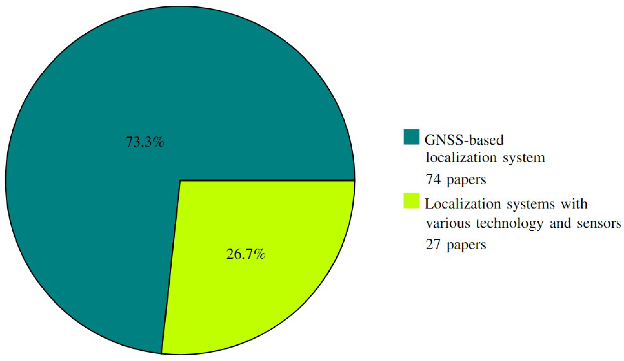
Figure 2.
Percentage of surveyed literature on integrity methods, categorized as being w. (with) PL and w.o (without) PL.
Figure 2.
Percentage of surveyed literature on integrity methods, categorized as being w. (with) PL and w.o (without) PL.
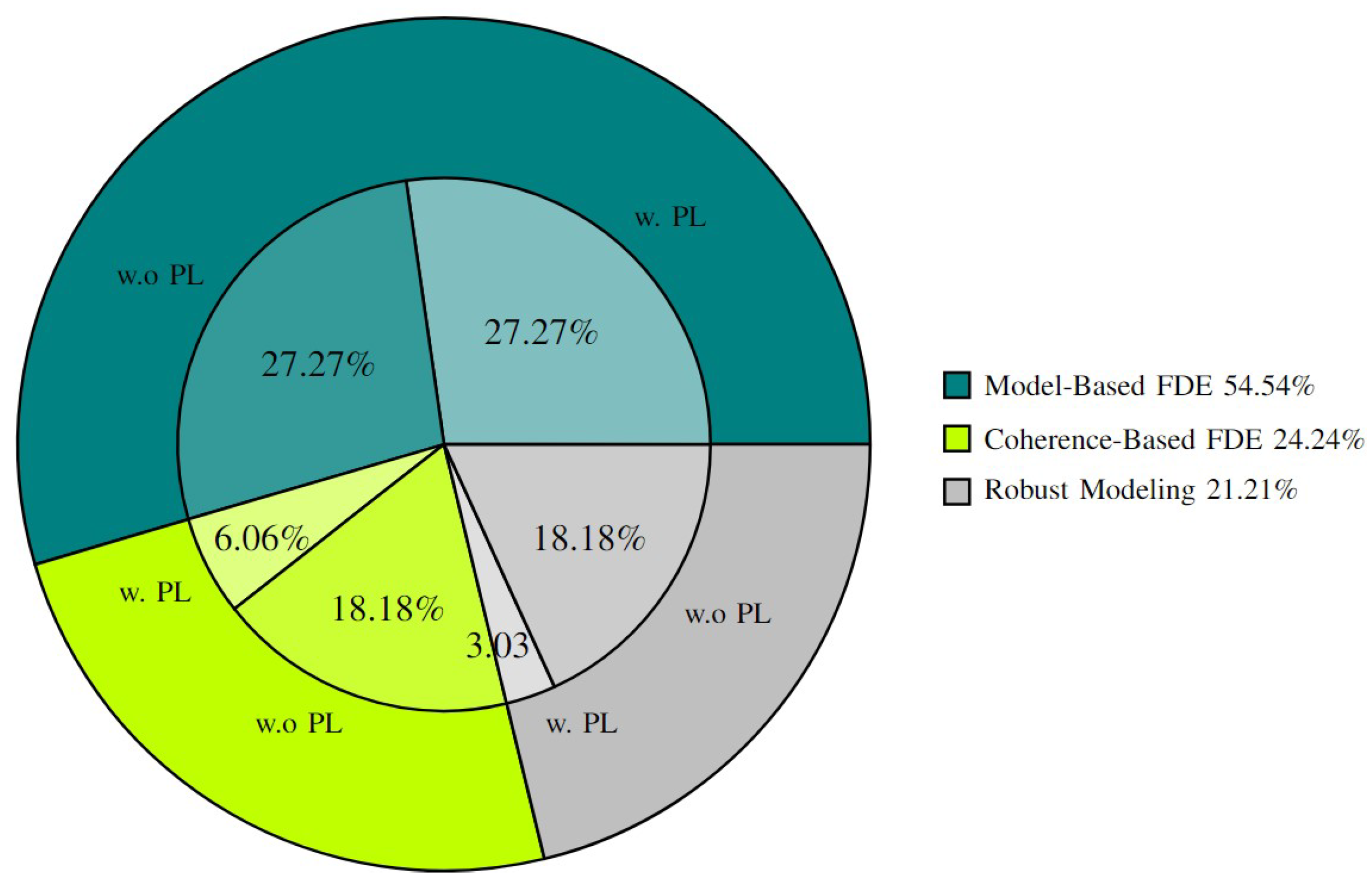
Figure 3.
Classification of Error Types.
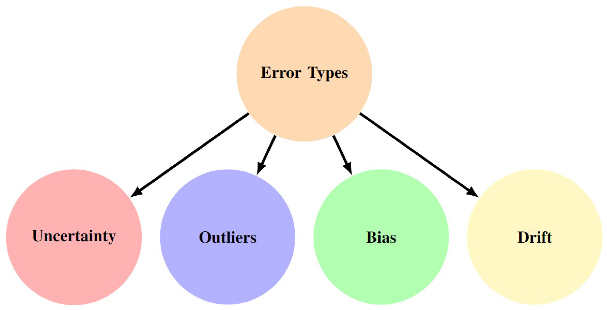
Figure 4.
Left: Histogram of LiDAR measurements at the true distance (5m). Right: Histogram of LiDAR measurements for the same true distance (5m) with m bias error (mean=4.5m).
Figure 4.
Left: Histogram of LiDAR measurements at the true distance (5m). Right: Histogram of LiDAR measurements for the same true distance (5m) with m bias error (mean=4.5m).
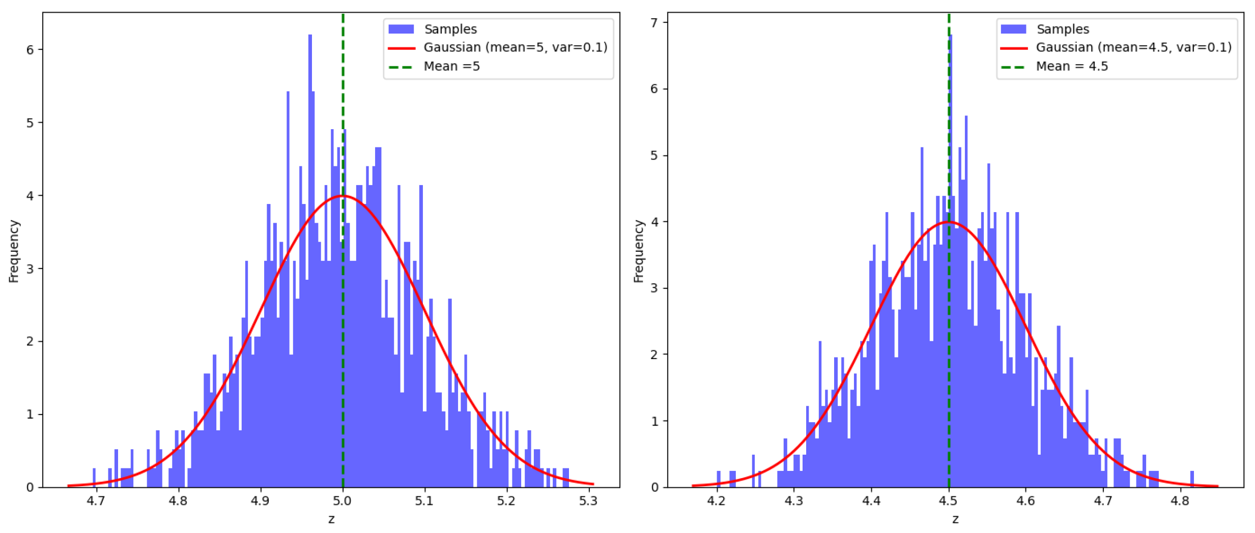
Figure 5.
Due to the drift error, the vehicle estimated path is constantly deviating from the truth path.
Figure 5.
Due to the drift error, the vehicle estimated path is constantly deviating from the truth path.
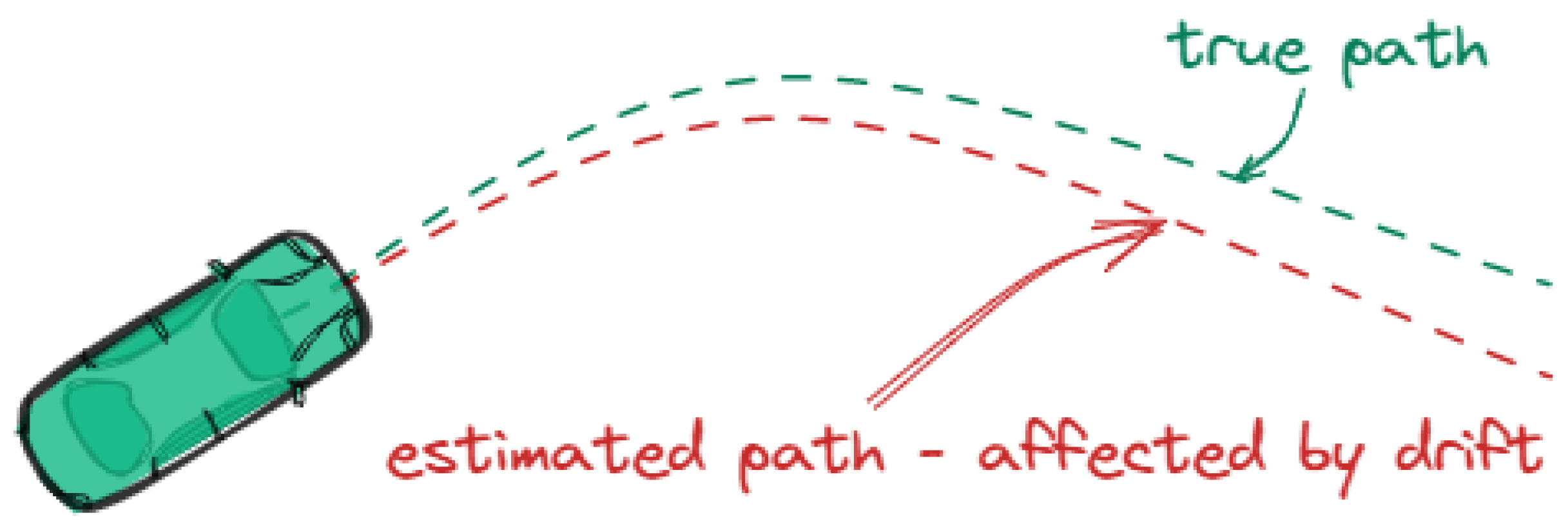
Figure 6.
The true and outlier distributions along with their combined PDF. The true distribution (blue) is a Gaussian with mean 5 and variance 0.1. Outlier distribution (green) is a uniform PDF, shifted to the right. Probability of encountering an outlier is set to 0.1.
Figure 6.
The true and outlier distributions along with their combined PDF. The true distribution (blue) is a Gaussian with mean 5 and variance 0.1. Outlier distribution (green) is a uniform PDF, shifted to the right. Probability of encountering an outlier is set to 0.1.
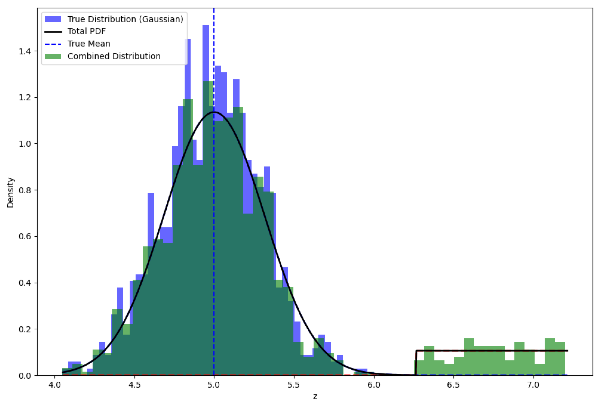
Figure 8.
RAIM methods classification.
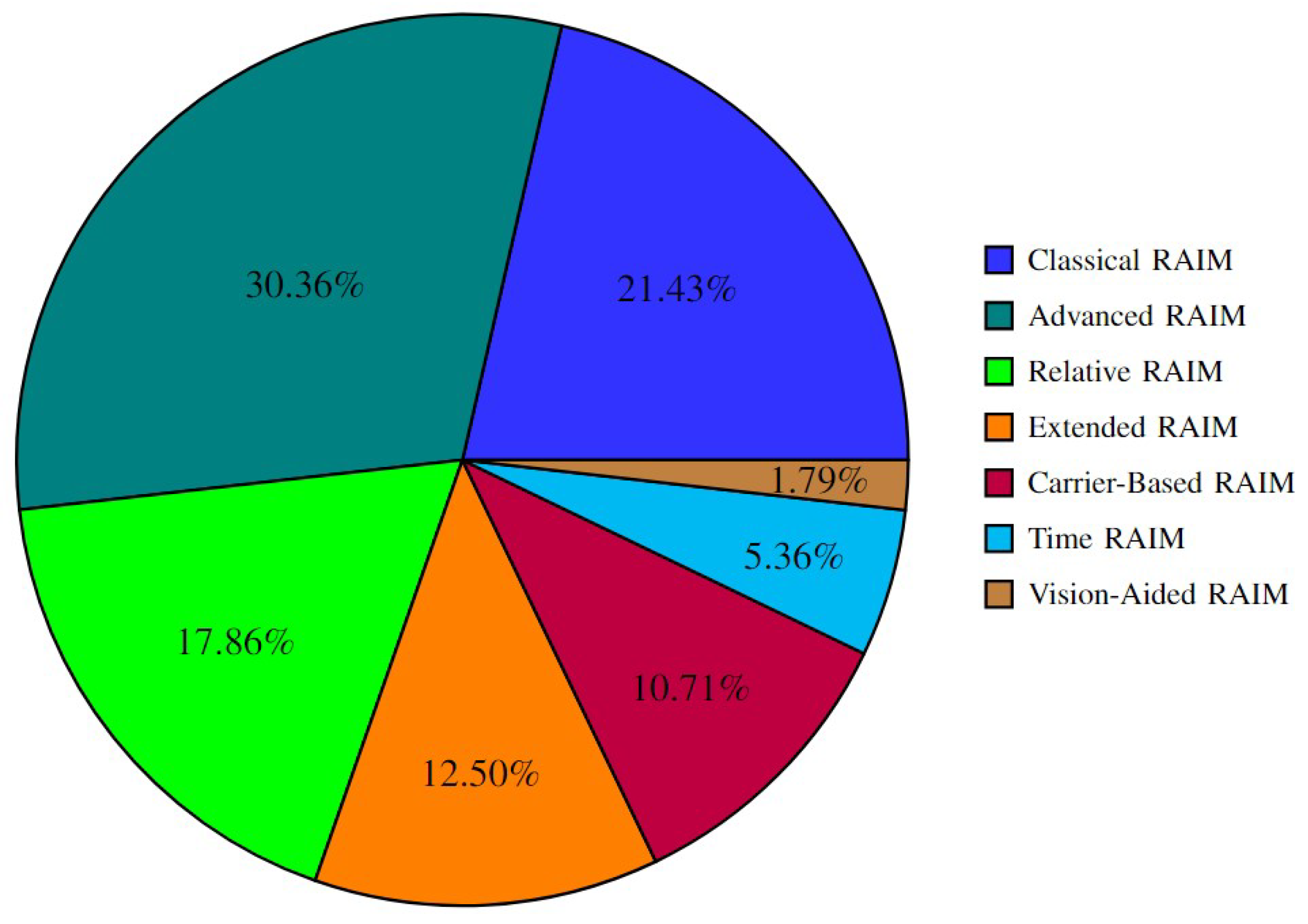
Figure 9.
Error distribution for a localization system at time t. The shaded regions indicate the probability that the error falls within those areas.
Figure 9.
Error distribution for a localization system at time t. The shaded regions indicate the probability that the error falls within those areas.
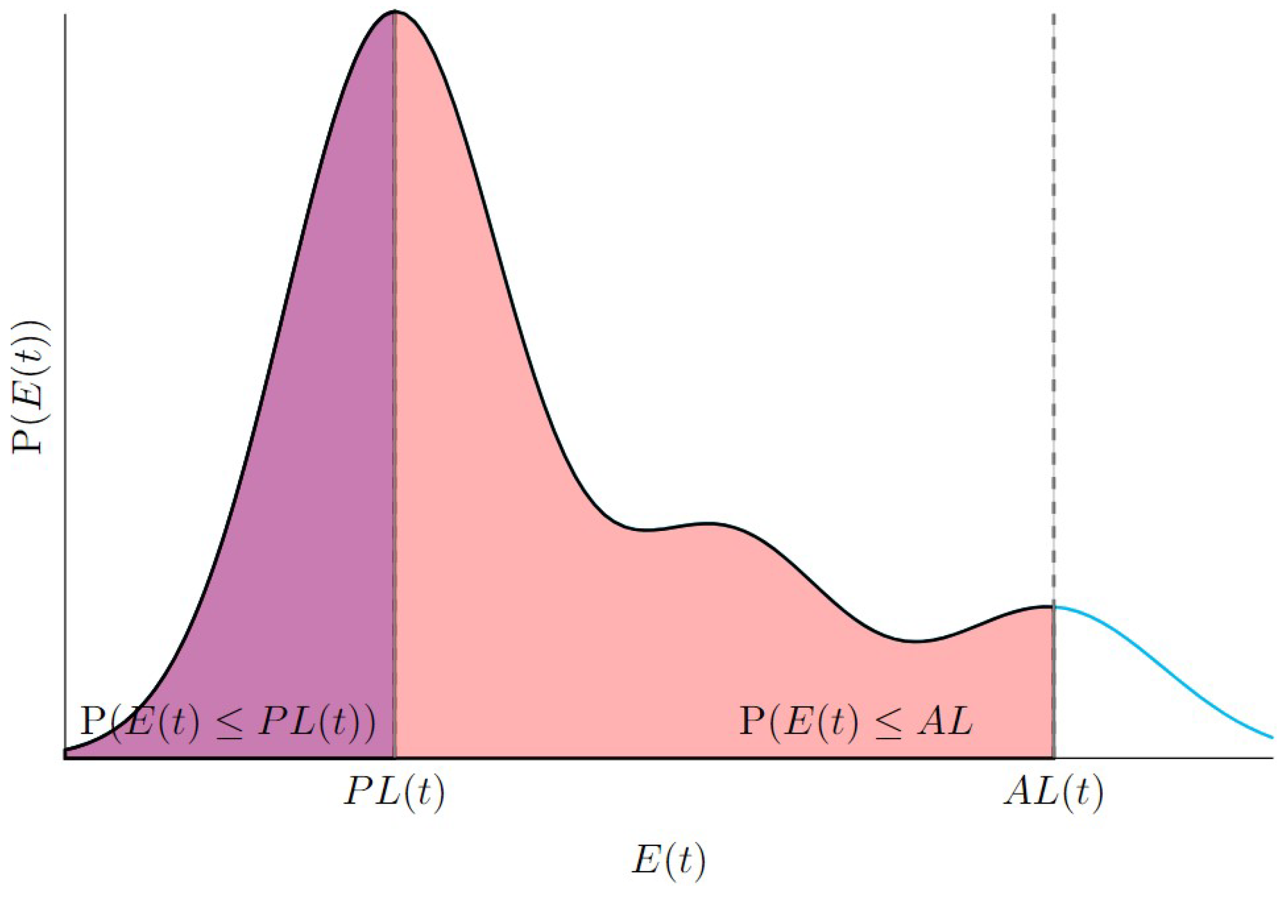
Figure 10.
Model-Based Fault Detection and Exclusion: A schematic representation illustrating the integration of predictive models for system behavior and localization systems.
Figure 10.
Model-Based Fault Detection and Exclusion: A schematic representation illustrating the integration of predictive models for system behavior and localization systems.
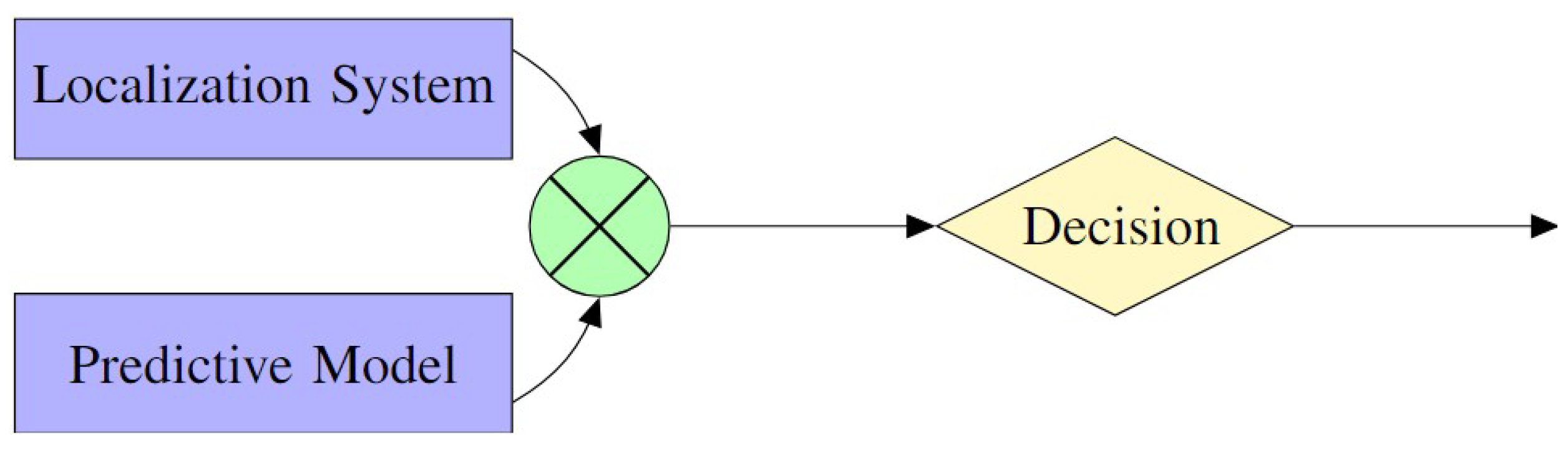
Figure 11.
Coherence-Based Fault Detection and Exclusion: The figure illustrates three localization systems (1, 2, and 3) undergoing coherence checks. Comparative analyses are performed between systems 1 and 2, 2 and 3, and 1 and 3 to identify any non-coherent behavior.
Figure 11.
Coherence-Based Fault Detection and Exclusion: The figure illustrates three localization systems (1, 2, and 3) undergoing coherence checks. Comparative analyses are performed between systems 1 and 2, 2 and 3, and 1 and 3 to identify any non-coherent behavior.
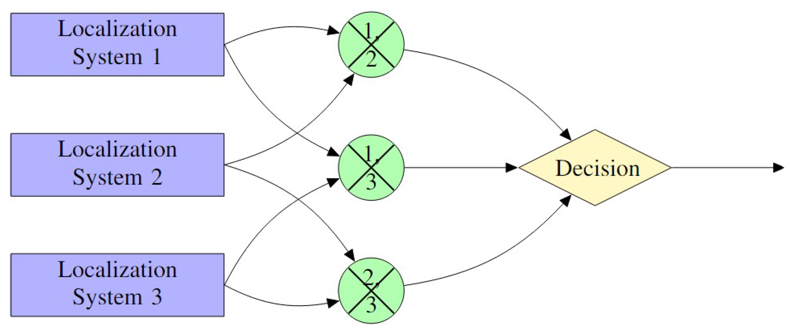
Figure 12.
Post-FDE Process in Localization Systems.
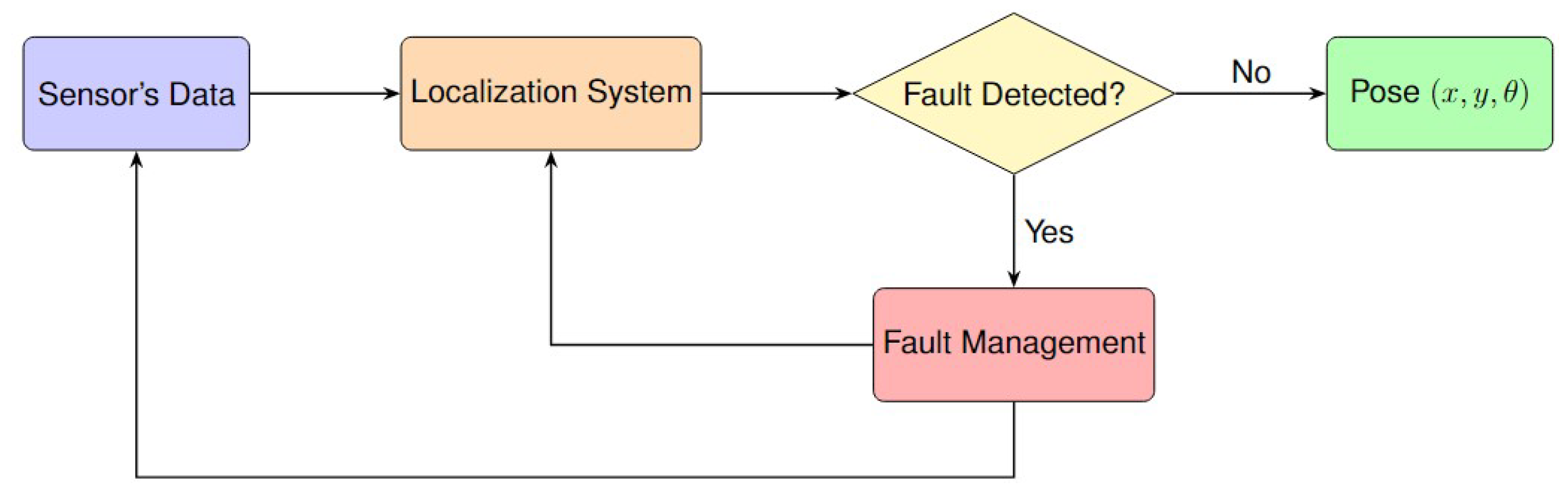
Figure 13.
Multi-sensor fusion with FDE uses camera measurements and the HD map as inputs. In the context of the information filter for multi-sensor fusion: Z denotes observations from GNSS or cameras, is the state vector, Y is the information matrix, and y is the information vector. and represent the information contributions from observation . This figure is adopted from [27].
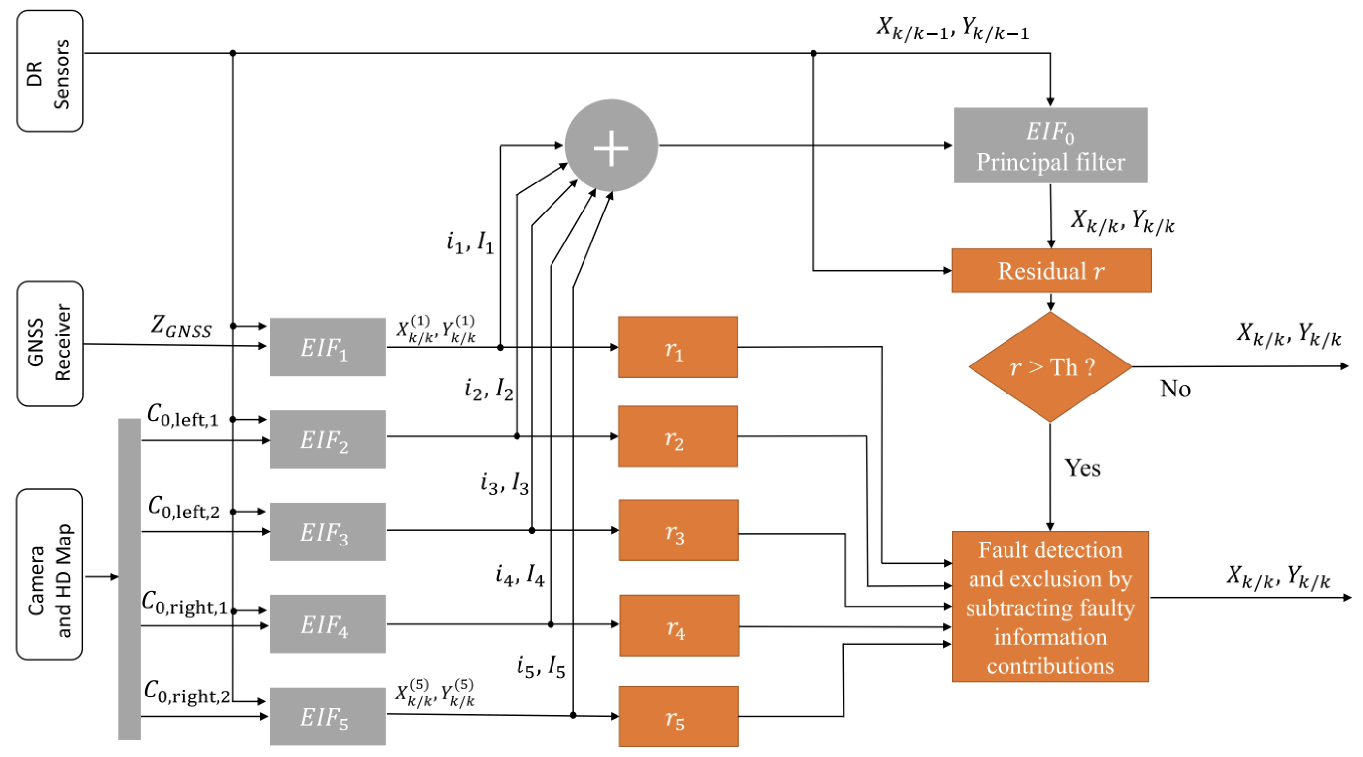
Figure 14.
Pre-FDE Process in Localization Systems.
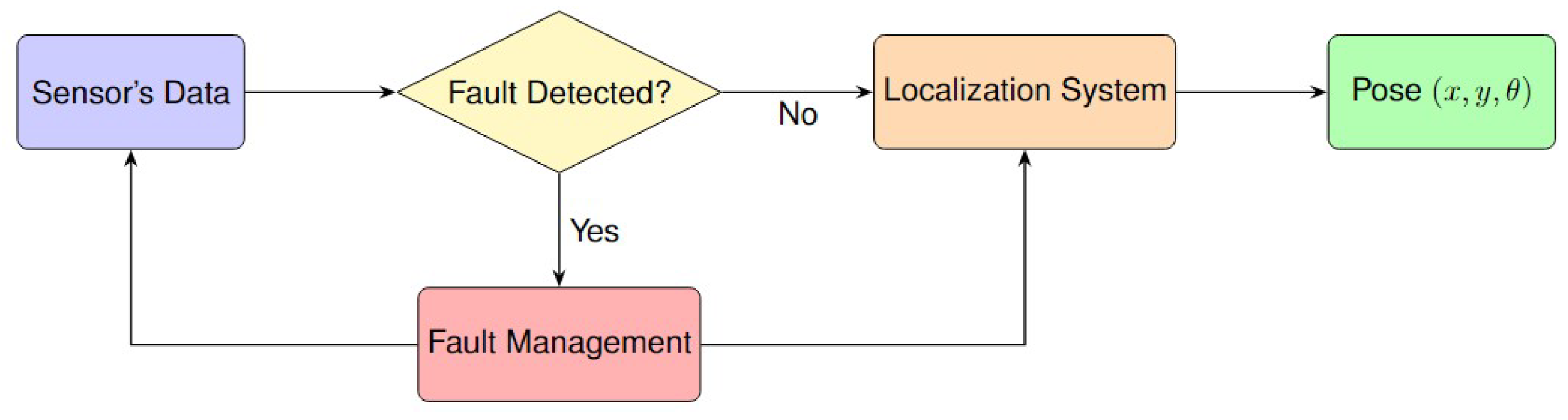
Figure 15.
The framework addresses GNSS faults with GMM Weighting with the voting scheme. This figure is adopted from [42].
Figure 15.
The framework addresses GNSS faults with GMM Weighting with the voting scheme. This figure is adopted from [42].
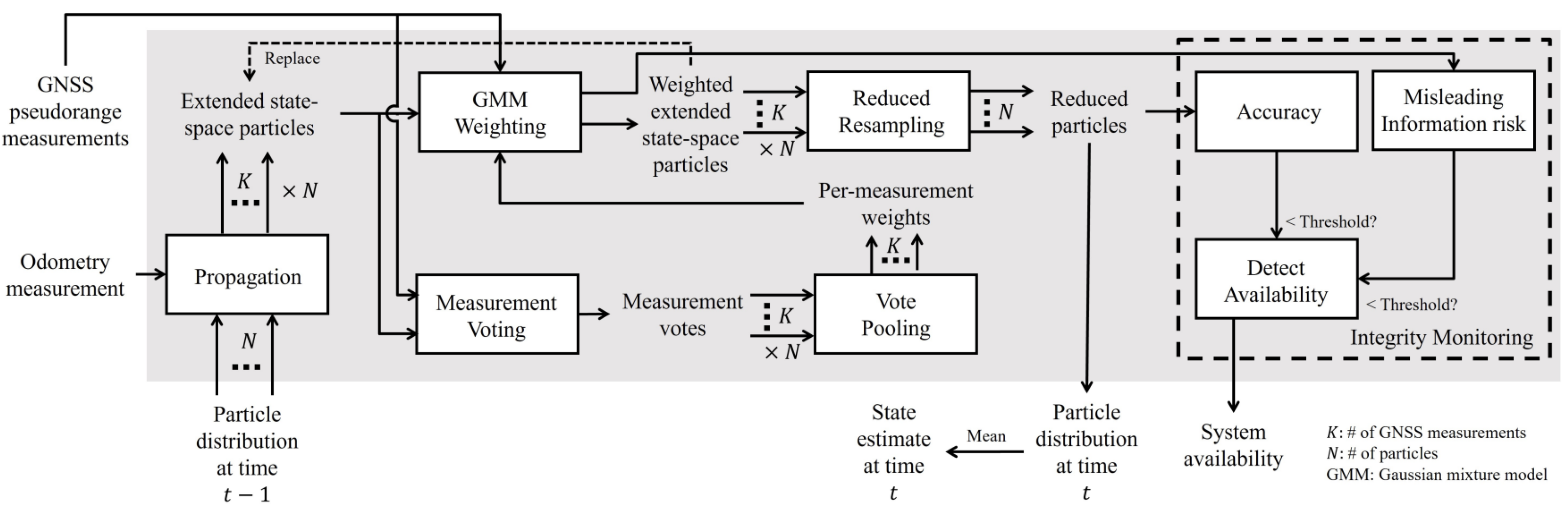
Figure 16.
The algorithm framework of using hierarchical clustering for FDE. This figure is adopted from [51].
Figure 16.
The algorithm framework of using hierarchical clustering for FDE. This figure is adopted from [51].
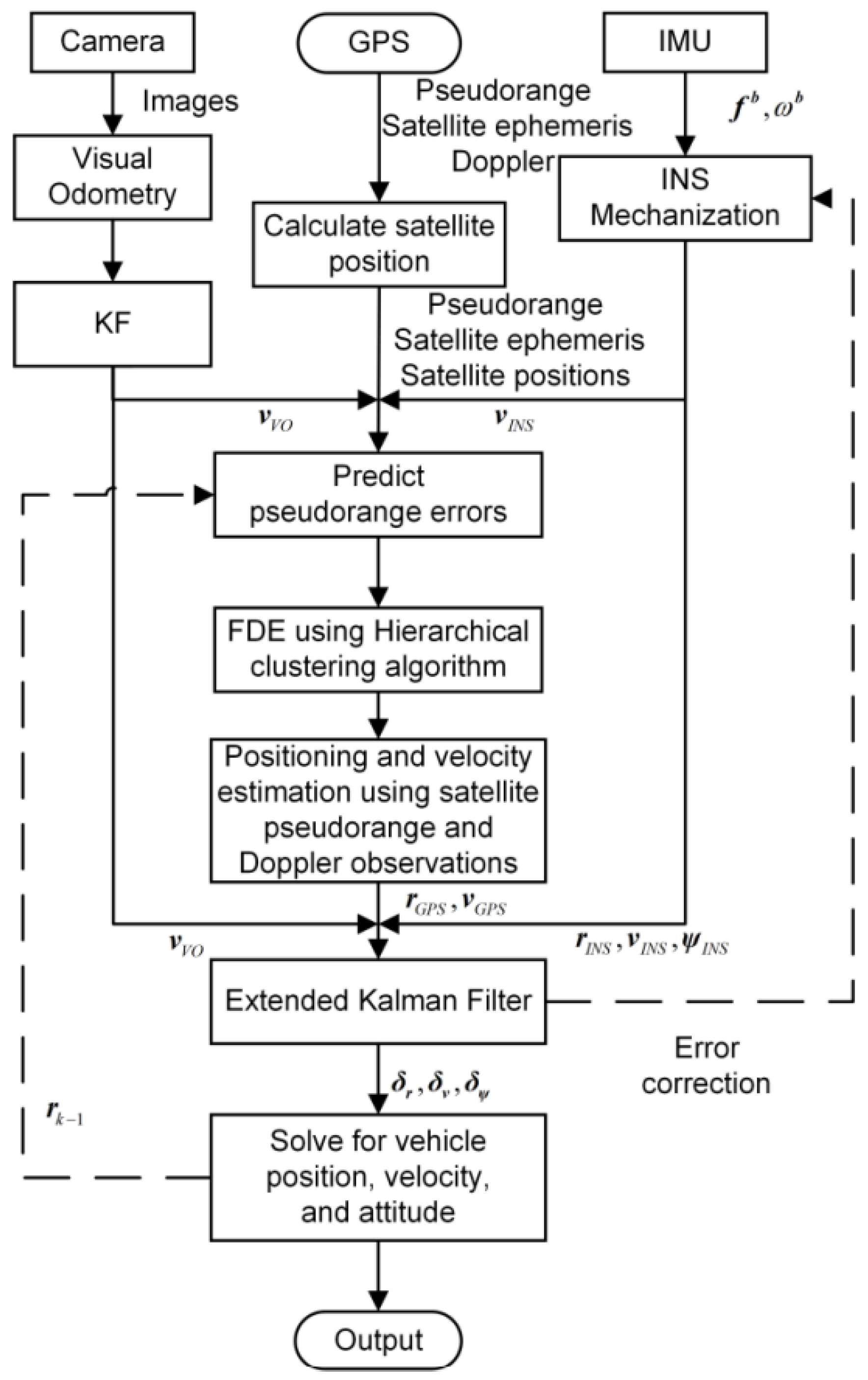
Figure 17.
Simultaneous FDE Process in Localization Systems.
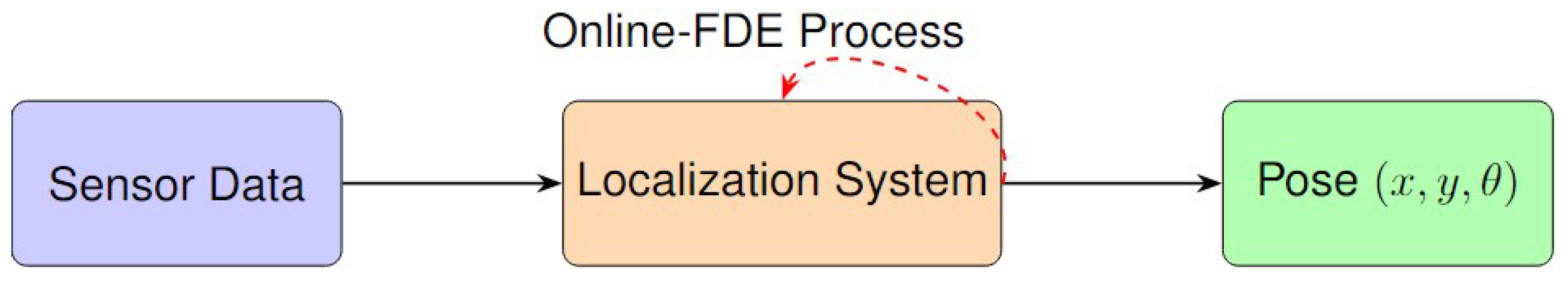
Figure 18.
GraphSLAM-based FDE algorithm detects and excludes multiple GPS faults. Orange stars represent GPS satellite landmarks. Blue triangles show the GPS receiver trajectory estimated by the GraphSLAM-based FDE. Gray triangles depict the vehicle trajectory estimated using only its motion model. This figure is adopted from [63].
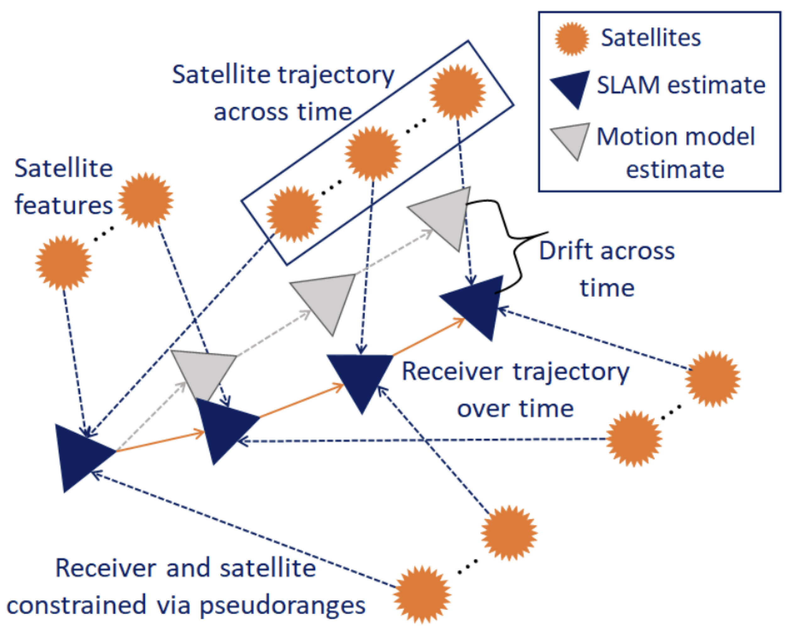
Figure 19.
An illustration of the GraphSLAM-based integrity monitoring approach combining GPS and visual data. This figure is adopted from [44].
Figure 19.
An illustration of the GraphSLAM-based integrity monitoring approach combining GPS and visual data. This figure is adopted from [44].
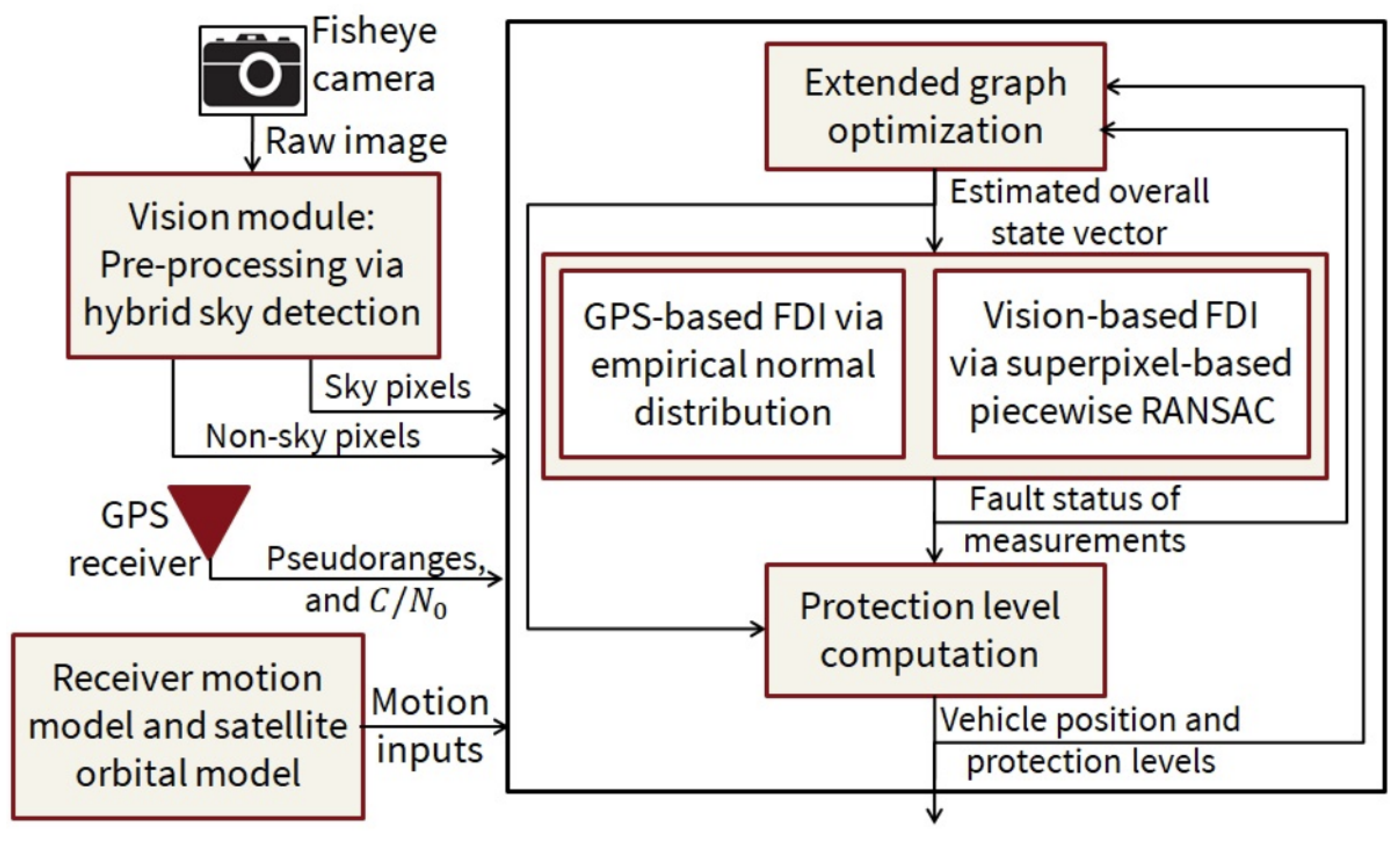
Figure 20.
Graphical model for estimating both the robot’s current pose and the reliability, , of this estimate. White nodes represent hidden variables, and gray nodes represent observable variables. The CNN uses sensor observations , the map and the pose to make a decision . Reliability is treated as a hidden variable and is estimated using the CNN’s decision and the control input . This figure is adopted from [48].

Figure 21.
Architecture of the deep neural network for estimating error distribution using CMRNet and correlation layers. A similar architecture, CovarianceNet, is used to produce covariance matrix parameters based on the translation error output. This figure is adopted from [46].
Figure 21.
Architecture of the deep neural network for estimating error distribution using CMRNet and correlation layers. A similar architecture, CovarianceNet, is used to produce covariance matrix parameters based on the translation error output. This figure is adopted from [46].
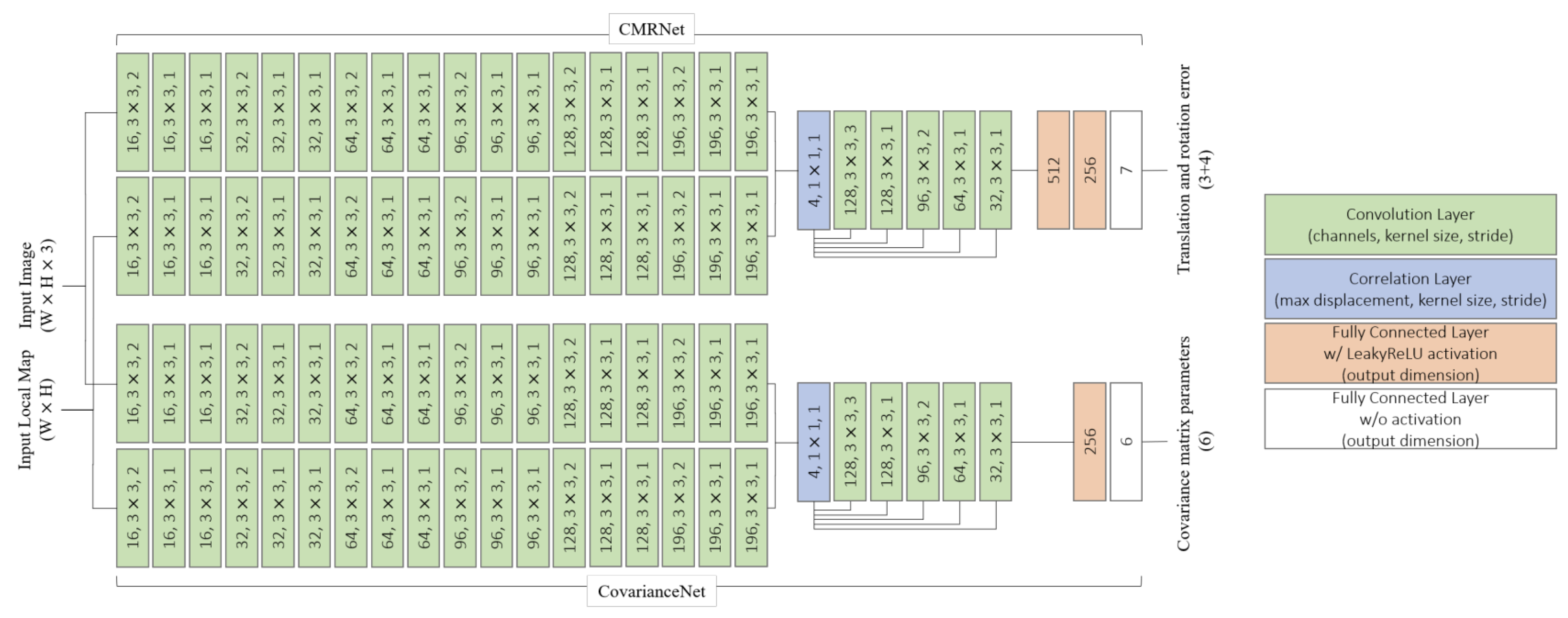
Figure 22.
Framework for assessing integrity by ensuring consistency across multiple data sources. This figure is adopted from [34].
Figure 22.
Framework for assessing integrity by ensuring consistency across multiple data sources. This figure is adopted from [34].
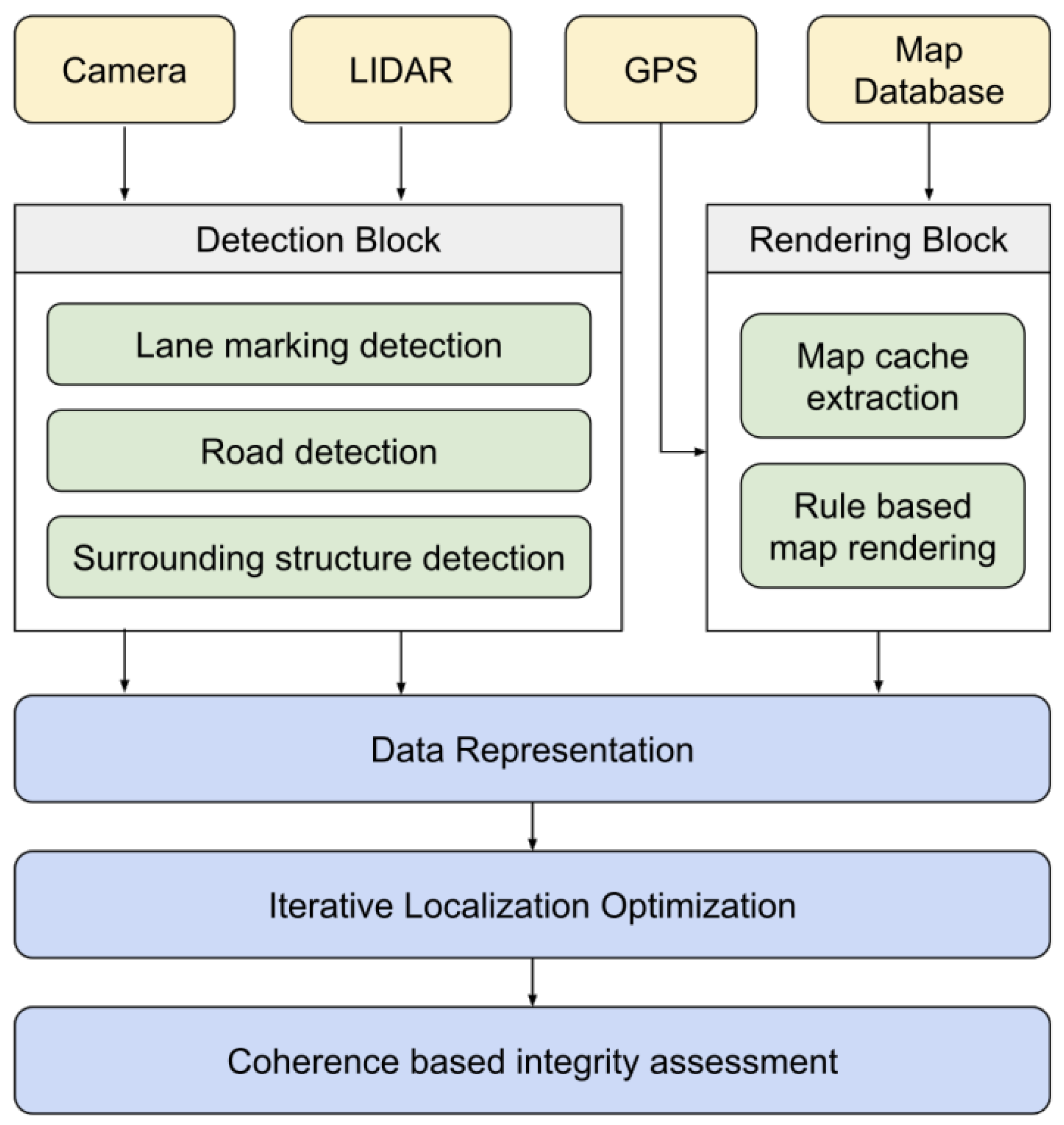
Figure 23.
Feature grid representing the vehicle’s localization. The grid shows data consistency across LiDAR, camera, and map sources. PL is indicated based on the variances of particle distributions. This figure is adopted from [34].
Figure 23.
Feature grid representing the vehicle’s localization. The grid shows data consistency across LiDAR, camera, and map sources. PL is indicated based on the variances of particle distributions. This figure is adopted from [34].
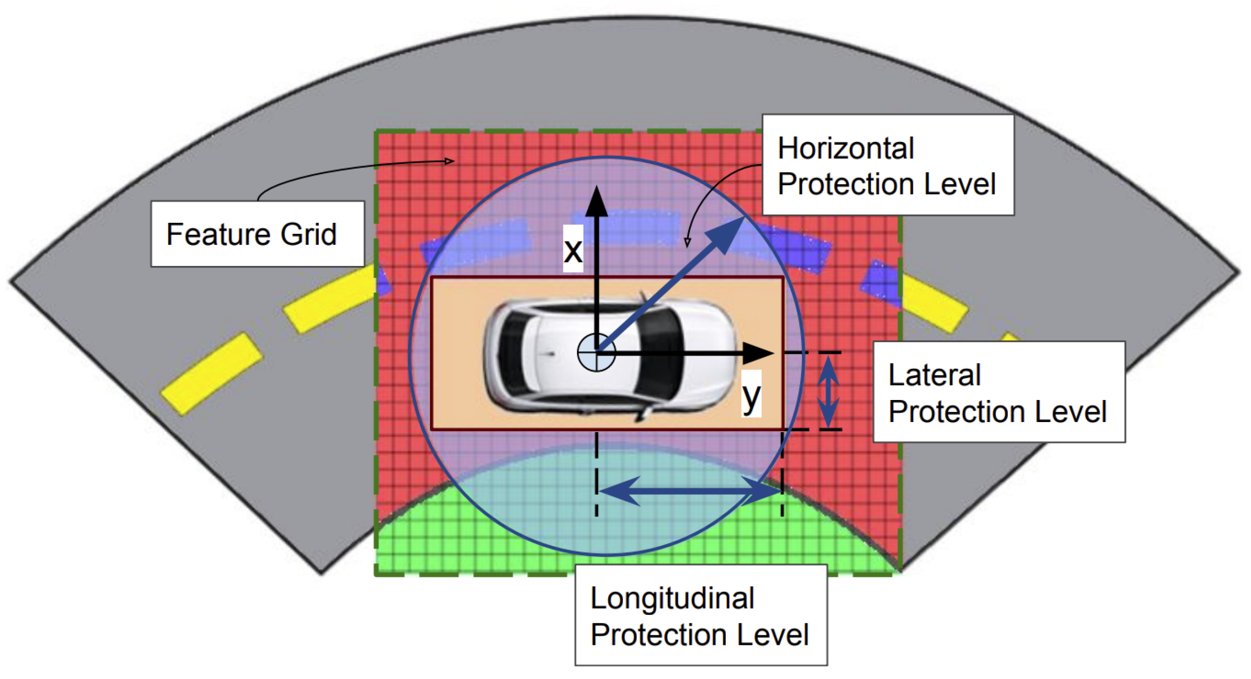
Figure 24.
The factor graph illustrates the pose estimation problem with various constraints. The poses to are represented as circular nodes, connected by different types of factors, indicated by colored filled circles. Odometry constraints (blue) are binary factors linking successive poses, representing the motion model between consecutive states. GPS constraints (red) are unary factors applied to specific poses, reflecting time-dependent GPS measurements. The map matching constraint (green) is a multi-node factor connecting all poses, ensuring alignment with a known map. In this figure we ignore the prior over initial state

Figure 25.
A binary weight is assigned to each loop closure constraint. When , the constraint remains active (top). When , the constraint is either disabled or removed (bottom). If these weights are treated as variables in the optimization process, the constraints can be adjusted or excluded during optimization. This figure is adopted from [117].
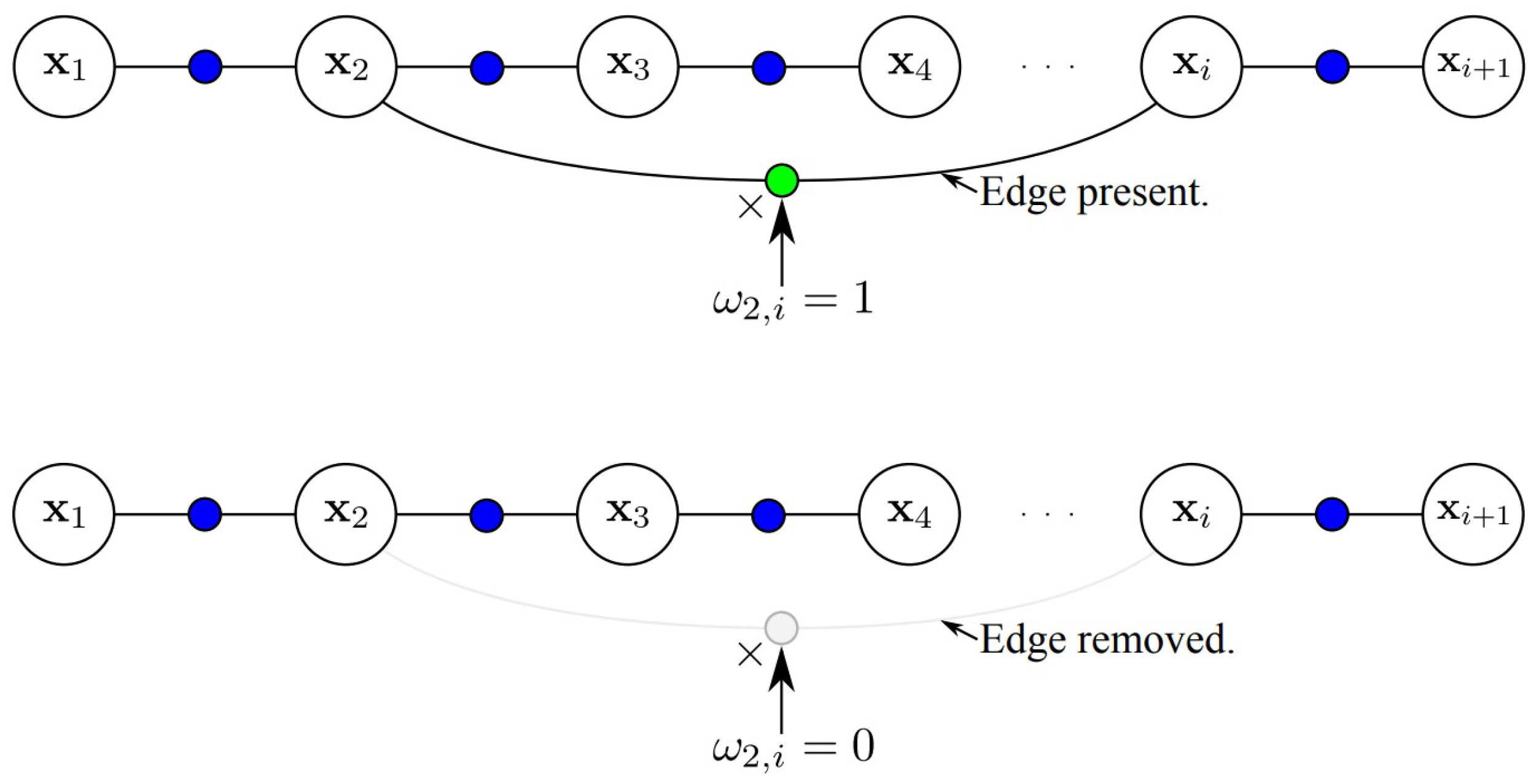
Figure 26.
The top plot displays the robust loss functions: L2 (Squared) loss, L1 (Absolute) loss, Huber loss, Cauchy loss, and Geman-McClure loss, each depicted with distinct line styles. The bottom plot shows the associated probability distributions, including Gaussian PDF for L2 loss, Laplacian PDF for L1 loss, and the specific distributions for the other kernels. Notably, Geman-McClure loss has no associated probability distribution, represented by a horizontal zero line.
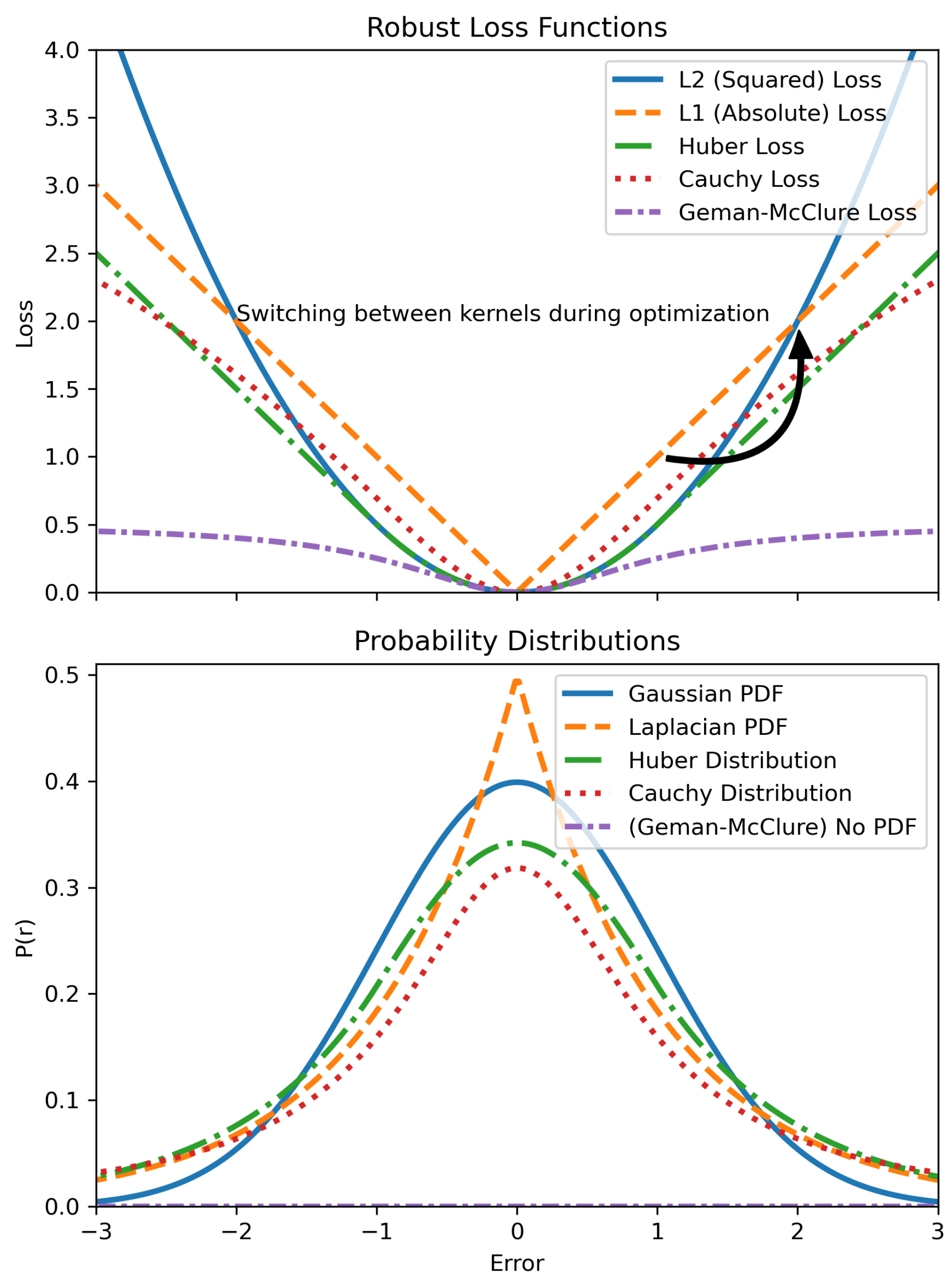

Table 1.
Summary of Model-Based Fault Detection and Exclusion Methods1.
| Reference | Algorithm | Fault Detection | Fault Exclusion | PL | Evaluation | Data | Sensor |
|---|---|---|---|---|---|---|---|
| [26,27,28] | EIF | Residual calculation using Mahalanobis distance | Compare residual with Chi-square distribution | Adjust covariance for estimated error using Student t-distribution | Calculate and compare with | Data gathered for city Rambouillet | Odometry, GNSS, Camera, HD map |
| [41] | t-EIF | Residual calculation using Kullback-Leibler Divergence | Compare residual with Chi-square and F-distributions | Compute with minimum degree of freedom | Calculate and compare with | Data gathered for town of Compiegne | Odometry, GPS, Camera, HP map |
| [42] | Particle filter | Use selection vector to vote for faulty measurement | Exclude faulty measurements | Use GMM to calculate error probability | Compare PE with PL | Simulation and Chemnitz data | GNSS, Odometry |
| [37,38] | EKF | Compute state residual error and compare with Chi-square distribution | Weight sensors based on residual error | Use Chi-square distribution for misdetection probability | N/A | Data acquired in urban context | Wheel speed sensors, yaw rate gyroscope, GPS |
| [36] | EKF | Feature-based approach | Dynamic thresholding | Use EKF error bound for error covariance | Miss detection and false alarm rate | Data acquired in urban canyons in Beijing | GNSS, INS, LiDAR |
| [43,44] | GraphSLAM | Test statistic computation, RANSAC | Batch test statistic computation | Perform worst-case failure slope analysis | Compare PE with PL | Data collected in alleyway of Stanford and semi-urban area of Champaign, Illinois | GPS, Fish eye camera |
| [45] | UKF | Hotelling’s test, Student t-distribution | Compare with a threshold | N/A | Compare with the standard UKF, adaptive UKF, adaptive UKF with the proposed FDE, and t-student adaptive UKF with the proposed FDE | Simulation and Highway experimental scenario | GNSS, IMU, velocity wheel sensor, steer angle, and position and azimuth using a SLAM |
| [31] | EKF | Parity space test | Compare residual with Chi-square distribution | Perform worst-case failure slope analysis | Compare slope of position error with respect to test statistics of parity space test | Simulation data | INS, Camera |
| [46] | CMRNet | Outlier weighting | N/A | Cumulative distribution function of a GMM | Bound gap, false alarm rate and failure rate | KITTI visual odometry dataset [47] | Camera |
1 All Vehicles are Ground Vehicles.
Table 2.
Summary of Model-Based Fault Detection and Exclusion Methods1.
| Reference | Algorithm | Fault Detection | Fault Exclusion | PL | Evaluation | Data | Sensor |
|---|---|---|---|---|---|---|---|
| [48] | RBPF + CNN | Detection of localization failure using CNN | N/A | N/A | Compare the results with AMCL2 | Simulation data and real indoor experiments | LiDAR |
| [49] | RBPF + CNN + LFM | Detection of localization failure using CNN | N/A | N/A | Compare the results with AMCL | Experimental environment and simulation environment | LiDAR |
| [50] | Free-space feature + MCL + IS | Detection of localization failure using MAE | N/A | N/A | Compare the results with AMCL | Simulation environment, Robotics 2D-Laser Datasets3 | LiDAR |
| [51] | VO-EKF | FDE using hierarchical clustering | Distance threshold between the pseudo range and the class center | N/A | Compare the result to the same system but without the FDE step | Field test Nanjing, Jiangsu, China, with the raw GNSS measurement | GPS, IMU, and binocular depth stereo camera |
| [52] | B-CIIF | Decision tree | Random forest | N/A | Accuracy of the decision tree and random forest | Experimental environment | Wheel encoders, IMU, LiDAR, and Marvelmind system |
1 All Vehicles are Ground Vehicles. 2 Augmented MCL [53,54,55]. 3 https://www.ipb.uni-bonn.de/datasets/
Table 3.
Summary of Model-Based Fault Detection and Exclusion Methods1.
| Reference | Algorithm | Fault Detection | Fault Exclusion | PL | Evaluation | Data | Sensor |
|---|---|---|---|---|---|---|---|
| [32,33] | ORB-SLAM2 | Parity space test | Compare residual with Chi-square distribution | Weighted covariance for sensor noise | Compare PL with | EuRoC dataset | Camera |
| [56] | B-CIIF | MLP | MLP | N/A | Accuracy of the MLPs | Experimental environment | Wheel encoders, IMU, LiDAR and marvelmind system |
| [57] | EIF | GKLD measure between prediction and update distribution | Use EIF bank for fault exclusion | N/A | Compare FDE with ground truth trajectory | Indoor environment | Wheel encoders, gyroscope, Kinect, LiDAR |
| [58] | EIF | Jensen Shannon divergence compared to Youden index of ROC curve | Signature matrix-based exclusion | Not specified | Data acquired by three Turtlebot3 | Experimental environment | Wheel encoders, IMU, LiDAR, marvelmind system |
Table 4.
Summary of Coherence-Based Fault Detection and Exclusion Methods1.
| Reference | Algorithm | Coherency Check | PL | Evaluation | Data | Sensor |
|---|---|---|---|---|---|---|
| [34] | Particle filter based map-matching | FG cell’s weight is used to weight each source and a threshold is applied to detect the incoherent source | HPL determined by the variances of particle distributions from each sensor combination used in the localization algorithm | Compare the HPL calculated by this method with historical values in [99] | KITTI with different scenarios | Cameras, LiDAR, GPS |
| [78] | 3D-NDT | MRF that exploits the full correlation between the sensor measurement | N/A | Root Mean Square error | SemanticKITTI dataset, and data acquired in Japanese public roads | LiDAR |
| *[85] | EKF | Cumulative Sum test | N/A | Observing when a faulty localization system is detected | Data acquired by the vehicle | Odometry and LiDAR |
| [87] | EKF-SLAM | Euclidean distances between positions from the EKFs and MarvelMind are measured and compared to a predetermined threshold | N/A | Compare the obtained pose with the ground truth trajectory | Acquired data through an experimental environment | EKF1 (encoder and LiDAR), EKF2 (encoder and gyroscope), MarvelMind |
| [35] | EKF | Euclidean distance between the two EKF systems output is calculated and compared with a threshold | N/A | False positive rate, no detection rate, detected errors rate, etc. | Data acquired in the city of Compiègne, France. Also, a simulation environment by using real data processed offline | INS, GPS, Wheels sensors, gyro-meter, and steering angle sensor |
| [88] | EKF | 8 residuals are generated and the one that exceeds for a specific number of time steps is excluded | N/A | False alarm | Simulation models | Gyroscopes and Wheels encoders |
| [89] | UIF | Extended NIS test where the sensor of increased residual is excluded | N/A | Compare with the ground truth trajectory | Real data acquired by an experimental vehicle | GPS, Stereoscopic System, LiDAR |
| [91,92] | Maximum Consensus | A consensus set for each pose candidate | Subset of grid cells that together account for a probability | N/A | Measurement data was recorded in an inner-city area with a dense building structure | LiDAR |
1 All Vehicles are Ground Vehicle
Table 5.
Summary of Robust Algorithms1.
| Reference | Algorithm | PL | Evaluation | Data | Sensor |
|---|---|---|---|---|---|
| [130] | RBPF R−EKF | Compute the maximum quantile for a specific TIR | Compare with base lines such as EKF with GNSS measurements only, EKF with MD-VO2 only and EKF with GNSS measurements and MD-VO | Hong Kong UrbanNav dataset [134] | GNSS, LiDAR, camera, and IMU |
| [114] | Factor Graph+ SC | N/A | Compare with the ground truth | Synthetic, like Manhattan, and real-world datasets, eg. Intel | Odometry and Camera |
| [115] | Factor Graph + SC | N/A | Compare with the ground truth | real data set | Odometry and GNSS receiver |
| [118] | Factor Graph+ DCS | N/A | Compare with the results of SC [115] | Synthetic, like Manhattan, and real-world datasets, eg. Intel | Odometry and Camera |
| [124] | Factor Graph + Self tuning M-Estimator | N/A | Compare the normalized squared error for different M-estimators | real data | Four monocular fish-eye cameras |
| [126] | ICP + Bundle Adjustment | N/A | Compare with static kernels, with [125] as well as SuMa3[135] | KITTI for ICP and CARLA simulator[136] for bundle adjustment | LiDAR for ICP, and camera for bundle adjustment |
| [127] | Factor Graph + EM | N/A | Chemnitz City and smartLoc [137] data set | N/A | GNSS receiver and odometry |
1 All Vehicles are Ground Vehicle. 2 Monocular-Depth Visual Odometry (MD-VO). 3 A dense mapping approach called Surfel-based Mapping (SuMa)
Disclaimer/Publisher’s Note: The statements, opinions and data contained in all publications are solely those of the individual author(s) and contributor(s) and not of MDPI and/or the editor(s). MDPI and/or the editor(s) disclaim responsibility for any injury to people or property resulting from any ideas, methods, instructions or products referred to in the content. |
© 2024 by the authors. Licensee MDPI, Basel, Switzerland. This article is an open access article distributed under the terms and conditions of the Creative Commons Attribution (CC BY) license (http://creativecommons.org/licenses/by/4.0/).
Copyright: This open access article is published under a Creative Commons CC BY 4.0 license, which permit the free download, distribution, and reuse, provided that the author and preprint are cited in any reuse.


