Submitted:
16 December 2024
Posted:
17 December 2024
You are already at the latest version
Abstract
This study examined atmospheric mechanisms affecting the East Bay Hills Fire (1991) in Oakland, California, using the Advanced Weather Research and Forecasting numerical model (WRF) and North American Regional Reanalysis (NARR) dataset. High-resolution WRF simulations at 16km were downscaled to 4km and 1km to analyze primary and secondary circulations at synoptic and meso-α/meso-β scales before the fire. Findings indicate that a ridge over the Great Basin and a trough off the Pacific coast created a strong pressure gradient over northern California, resulting in favorable meso-α conditions for the hot, dry northeasterly winds, known as "Diablo winds," that initiated the wildfire. Additionally, mountain waves from the jet stream enhanced the sinking air on the Sierra Nevada's western side. The main conclusion is that jet circulations did not directly transport warm, dry air to the fire but established a vertical atmospheric structure conducive to wave amplification and breaking, and downward dry air fluxes, leading to the necessary warm and dry low-level air for the fire. The Hot-Dry-Windy (HDW) fire weather index also indicated how favorable the environment was for this tragic event.
Keywords:
Diablo Winds
; East Bay Hills Fire (1991)
; Hot-Dry-Windy (HDW)
; Hydraulic Mechanism
; Resonant Amplification Mechanism
; Weather Research and Forecasting (WRF)
1. Introduction
Terrain-induced winds often lead to major wildfires in California [1,2,3]. Diablo, Santa Ana, and Sundowner winds have caused major wildfires such as the East Bay Hills Fire (1991), Cedar Fire (2003), and Sherpa Fire (2016), respectively. This study will focus on the orographic effects of Diablo wind on the East Bay Hills Fire [4]. Diablo wind is a hot and dry northeasterly wind that occurs in the San Francisco Bay area during the fall [5], similar to Santa Ana winds in Southern California. Diablo winds result from a high-pressure system over the great basin of the inland western states and an offshore low-pressure system that causes the wind to flow from northeast to southwest, decreasing relative humidity and increasing wind speed [6].
In October 1991, the East Bay Hills Fire broke out in the Oakland-Berkeley Hills area near the San Francisco Bay. Before the fire, an easterly flow pattern produced high temperatures and low humidity levels. The fire was spread by gusty winds, leading to 25 deaths, 150 injuries, and at least 5,000 people without homes. Over 3,354 single-family dwellings, 456 apartments, and 2,000 cars were destroyed, making it the most expensive wildland-urban fire in US history at that time. Huang et al. [1] used data and simulations to study the synoptic-scale and mesoscale environment during the Cedar Fire (2009). They identified three stages of interaction: In stage I, dry air was transported from the upper troposphere to the surface due to a meso-alpha-scale subsidence region. In stage II, the jet streak intensified and caused strong northeast winds to move the dry air toward California's coast. In stage III, the interaction of a wave-induced critical level and strong upper-level sinking air motion led to the formation of Santa Ana winds. We will investigate whether a similar interaction occurred during the East Bay Hills Fire (1991) and whether a jet streak transported dry air to the surface. Huang et al. [1] used NHMASS data, while we used NARR data for backward trajectory. We aim to analyze synoptic-scale and mesoscale environments and test a new fire weather index (HDW) [7]. We calculated the HDW using WRF simulated results to identify the days when meso-α scale weather activity contributed to the East Bay Hill Fire (1991). The HDW uses fundamental principles of observed favorable fire weather environment to identify the best meteorological variables that control wildfires at the synoptic and meso-alpha scales.
Srock et al. [7] introduced a new variable for assessing the risk of heat and drought waves (HDW) by combining atmospheric heat and moisture. The fire community commonly uses relative humidity (RH), which includes temperature as a variable. The vapor pressure deficit (VPD) variable is used to assess the amount of possible evaporation for HDW. A larger difference between es and e at a given temperature implies higher evaporation rates in plant environments. The VPD variable has been widely used in environmental science for assessing evapotranspiration rates [8,9,10].
where VPD is the vapor pressure deficit, T is the temperature, q is the specific humidity es(T) is the saturation vapor pressure at temperature T, e(q) is the actual vapor pressure based on the specific humidity q. A larger (smaller) VPD directly correlates to a faster (slower) evaporation rate, which is, in turn, associated with a greater (lesser) potential for the atmosphere to affect a fire. Hence, they propose the equation to calculate the HDW as wind speed (U) times the VPD:
where HDW is the Hot-Dry-Windy Index, U is the wind speed, and VPD (T, q) is the vapor pressure deficit. Strong downslope winds are linked to wildfires, and their dynamics must be understood to manage and prevent related fires. Two major mechanisms that intensify downslope winds are the resonant amplification mechanism [11] (hereafter referred to as CP84) and the hydraulic mechanism [12] (hereafter referred to as S85). This study will investigate the formation mechanisms of downslope winds related to the East Bay Hills Fire (1991) using WRF simulation. The study will measure wave breaking with simulated winds and isentropes. Unlike Lin and Wang's [13] idealized simulation, this study uses actual simulated results. Most California wildfires occur due to strong downslope winds, like the Diablo wind, which caused the East Bay Hills Fire in 1991. The National Weather Service has a conceptual model explaining how Diablo winds cause wildfires (https://en.wikipedia.org/wiki/Diablo_wind).
VPD (T, q) = es(T) – e(q)
HDW = U * VPD (T, q)
Based on the conceptual model explained above for Diablo winds, we propose to enhance our understanding of the key processes that led to the mesoscale environment conducive to the formation of the East Bay Hills fire by addressing the following questions: (a) How does the high pressure circulation over the Great Basin force the air to go over the Sierra Nevada? (b) Could the downslope motion be (i) enhanced by the sinking air motion associated with an upper-level jet streak [1], (ii) produced by the resonant amplification mechanism [11] (CP84), and/or (iii) Smith's hydraulic jump mechanism? [12] (S85) and (c) Will the hot, dry, and windy air blowing from Sierra Nevada's downslope maintain the same thermodynamic characteristics over the Central Valley of California? This study aims to address these questions by utilizing analyzed data from the North American Regional Reanalysis (NARR) dataset, focusing on the interaction between the mesoscale and synoptic scale environments. We will employ the WRF model to investigate the hot, dry, and windy airmass affecting California's Central Valley. Both NARR and WRF will also aid in exploring the mechanisms behind the severe downslope winds in the western Sierra Nevada. Section 2 will cover the model description and experimental design, while section 3 will focus on examining the synoptic and mesoscale environments favorable for wildfire occurrence. In section 4, we will delve into the mechanisms of severe downslope winds on the lee slope of the Sierra Nevada. Next, section 5 will analyze how the hot, dry, and windy air propagates across California's Central Valley and estimate HDW. Lastly, section 6 will offer concluding remarks.
2. Simulation Methodology
The WRF model version 3.9 [14] was adopted for the East Bay Hills Fire (1991) numerical simulations in Oakland, California. The WRF model is a numerical weather prediction system designed to understand mesoscale weather phenomena better. To achieve this, the model incorporates either initial idealized data or real-time data for better operational weather prediction. WRF is a fully compressible, three-dimensional model that uses terrain-following vertical coordinates with stretched grid resolution. It also includes one-way or two-way multiple nesting capability, along with a variety of options for upper and lateral boundary conditions. To test the ability of the WRF model to simulate the East Bay Hills Fire event, the methodology of Huang et al. [1] was employed. In their study, Huang et al. [1] analyzed the October 2003 extreme fire event in Southern California using the non-hydrostatic (NHMASS) version 6.3 of the Mesoscale Atmospheric Simulation System (MASS). We performed sensitivity tests utilizing data from the National Centers for Environmental Prediction (NCEP), NARR, and the European Centre for Medium-Range Weather Forecasts (ECMWF) to initialize the WRF model. Our findings indicate that the model initialized with ECMWF data is more precise than the other two datasets compared to the observed data. As a result, we utilized the ERA-Interim reanalysis data from ECMWF to initialize the WRF model for the control simulation. The domain comprised of three grids with varying resolutions: 16 km (D1), 4 km (D2), and 1 km (D3). We utilized two-way interactions to facilitate interactions among the lateral boundary conditions for the D1 domain (16km) and nested grid two-way interactions at the D2 domain (4km) and D3 (1km) domains (Figure 1). D1 domain covers the western United States and part of Canada to reproduce the synoptic flow in which the mesoscale environment is embedded. The southwestern states, including California, Nevada, Utah, and Arizona, fall within the jurisdiction of the D2 domain. The purpose of the D3 domain is to collect data on the meso-β-scale characteristics of the airflow over the San Francisco Bay Area, which the fire has significantly impacted. The simulations for domains D1, D2, and D3 run in parallel, starting at 10/19/12Z, 10/20/00Z, and 10/20/12Z, respectively, and ending at 10/21/12Z. This approach mimics Huang et al.'s [1] study. To capture very fine vertical motions, we use a domain top of 10 hPa and 75 stretched vertical levels, and the domains have grid points of 260 x 277 (D1), 457 x 437 (D2), and 597 x 609 (D3). The time step intervals are 60, 15, and 3.7 s for domains D1, D2, and D3, respectively.
The simulations incorporate various options for physics parameterization, such as the Purdue Lin microphysics scheme [15], Kain-Fritsch cumulus scheme [16], Mellor-Yamada-Janjic scheme for the planetary boundary layer [17], Rapid Radiative Transfer Model (RRTM) longwave radiation physics scheme [18], RRTM for General Circulations Models (RRTMG), and shortwave radiation physics scheme [19]. RRTM is the most precise for single-column calculations, while RRTMG is efficient with minimal loss of accuracy for General Circulation Model (GCM) applications. The Noah Land-Surface Model is the chosen land surface model. It's an all-in-one scheme developed by NCEP/NCAR/AFWA, featuring a four-layer soil temperature and moisture function, fractional snow cover, and frozen soil physics. The surface layer utilizes the Monin-Obukhov (Janjic Eta) Similarity scheme, which is based on similarity theory and includes viscous sublayers over solid surfaces and water points.
3. Synoptic-Scale and Mesoscale Analyses
3.1. Synoptic Environment
During October 19 - 20, 1991, a strong upper-level ridge along the West Coast produced warm and dry weather conditions over northern California (Figure 2). Marine layer clouds are low-altitude stratus clouds that form over the adjacent ocean waters. They are formed due to ocean water’s cold surface temperatures, increasing air temperatures with height and producing temperature inversion. The air below the inversion is called the marine layer. The depth of the marine layer depends upon the large-scale weather patterns that pass high overhead. The marine layer clouds often reach their maximum extent around sunrise when the surface reaches a minimum temperature. The colder surface temperatures enhance the inversion layer and then increase the marine layer depth.
As the day progresses, sunlight penetrates the clouds and warms the surface and air above. This warming decreases the relative humidity of the cloudy air, and clouds begin to evaporate. Strong winds above the clouds can mix in drier air, leading to more evaporation, then the marine layer will dissipate [20].
The slow destruction of the marine layer gave rise to drier and warmer air near the coastal areas, and the increasing temperatures lowered mean sea level pressures (MSLP) along the coast. This lowering of the MSLP along the California coast produced an intensifying south to southwestward-directed pressure gradient across northern California through the weekend of October 19th and 20th (Figure 3). From the MSLP in Figure 3, the pressure difference between the San Francisco Bay (SFB) area and northern Nevada (NNV) was about 6-10 hPa from 10/19/00Z to 10/19/12Z. Twenty-four hours later, the MSLP along the California coast had fallen by 4 hPa or more. At the same time, the MSLP difference between the San Francisco Bay area and northern Nevada had increased to 10-14 hPa (Figure 3).
The Oakland radiosonde ascent (Figure 4) indicates the presence of extremely dry air, which can be attributed to subsidence on 10/20/00Z. There was a low-level maximum of approximately 18kts in the northeasterly wind at 4000 feet (approx. 900 hPa). During the early morning, 5:00 PDT October 20 (10/20/12Z), some marine air at the surface moved eastward near Oakland, but very dry conditions continued aloft, and the easterly winds increased (Figure 4). For the most part, over northern California, the MSLP continued to fall during the night until around 5:00 PDT on October 20 (10/20/12Z). During this period, the pressure difference between the San Francisco Bay area and northern Nevada reached a maximum of 14 hPa (Figure 3).
At 5:00 AM PDT on October 20th, a comparison was made between the 500mb heights over San Francisco Bay and those from October 19th at 5:00 PM PDT. The results showed that the heights were lower due to the retrogression of the upper ridge. This retrogression supported more north-to-northeasterly flow at upper levels, as evidenced by figures 4b and 4c. Consequently, the upper-level flow over the Great Basin became stronger. At the same time, the increasing Intermountain West MSLP gradient intensified the low-level winds generated by the low-level southwestward-directed/offshore pressure gradients. On October 20th at 11:00 AM PDT, the National Weather Service (NWS) reported that the shallow marine layer near Oakland's surface dissipated. This finding suggests that the observed changes in the 500mb heights over San Francisco Bay from the previous day's measurements may have contributed to the dissipation of the shallow marine layer. The surface wind increased drastically, the temperature increased ~13oC in one hour (the highest temperature recorded for the day), and the dew point temperature fell ~9oC [21]. These phenomena coincided with the initial blowup of the main fire complex at this time. The MSLP gradient lowered during the daytime as the northern Rockies and Great Basin surface pressures dropped. Eventually, as the MSLP gradient lowered around the San Francisco Bay (SFB) area, the support for northeasterly winds decreased during the day. Nevertheless, the strong winds continued in Oakland into the evening, and this can be seen in the observed Skew-T plot showing moderately strong winds (15-20 knots) at the surface and dissipation of the marine layer (Figure 4d). Afterward, the pressure gradient decreased, and the surface winds in the East Bay Hills area weakened substantially and turned to the west-northwest by 10/21/12Z (Figure 4e). Later, the west-northwesterly wind shifted to a southwesterly wind, causing a moist marine layer to enter the East Bay Hills fire area during the day, which helped lessen the fire (Figure 4f).
3.2. Mesoscale Environment
The WRF simulated 4km resolution grid variables are used to analyze how hot, dry, and windy the environment was during the East Bay Hills fire. First, we investigate how windy it is using isotach plots at different levels and times. According to the Oakland Fire Department [6], the fire started at around 10:53 PDT (1753 UTC) on Sunday, October 20, 1991. The fire continued to intensify until 19:30 PDT on October 20 (0230 UTC, Oct 21). The fire started to diminish as winds shifted from northeasterly to northwesterly. Concerning the fire start and end times, we analyze the WRF simulated data from 1200 UTC October 19, 1991, to 1200 UTC October 21, 1991. Figure 5 shows the wind speed at various levels during the fire event's start time (between 10/20/15Z and 10/20/18Z). At the fire location (denoted with a black dot), the winds from the surface up to 250 hPa are predominantly northeasterly. In connection with the observed Skew-T plot (Figure 4c and 4d), the winds are also northeasterly from the surface to about 200 hPa level during 10/20/12Z and 10/21/00Z, which the event’s start time falls within. According to the simulated data obtained from WRF, the surface winds were moderately strong (12-14 ms-1) from 10/20/15Z to 10/20/18Z, creating a highly favorable environment for the spread of fire (Figure 5).
Later, at the 850 and 700 hPa levels, the northeasterly wind flow changed southwesterly (Figure 6), which advected moisture to the fire location from 10/21/06Z to 10/21/12Z. Compared with the observed Skew-T plot, during 10/22/00Z from the surface to 700 hPa, the winds are primarily southwesterlies (Figure 4f). Although the southwesterly wind in the WRF simulation is seen earlier than in the observed Skew-T plot, both simulated and observed plots show similar wind directions during the start and end of the East Bay Hills Fire in Oakland. Between 10/21/06Z and 10/21/12Z, surface winds remain weak and variable, while southwest winds at 850 and 700 hPa introduce moisture to help extinguish the fire.
The RH profile near the fire site indicates a moist surface (RH at 60-70%) and drier conditions at 700 and 850 hPa on 10/20/15Z (Figure 7). This aligns with the presence of moist marine air near the surface, as depicted in the skew-T diagram (Figure 4d). Following the fire's intensification at 10/20/18Z, the surface humidity drops significantly to around 20-30%, with the 850 and 700 hPa levels also showing RH between 10-20% (Figure 7 and Figure 8). Consequently, the atmosphere became dry from the surface to the 700 hPa level, fostering a supportive environment for wildland fire formation. The surface temperature rose consistently from 22-28°C (72-82°F) between 10/20/15Z and 10/20/18Z, as illustrated in Figure 9, which coincided with the wildland fire event's intensification. On 10/21/06Z, warm surface temperatures (24-28°C) persisted until 10/21/12Z, when temperatures began to drop to 18-26°C (Figure 10), paralleled by a rise in surface relative humidity from 40-50% (Figure 8). The decrease in temperature and relative humidity increase can be partly linked to a change in wind direction from northeast to southwest, facilitating moisture movement into the fire area and reducing the fire's intensity.
4. The Formation Mechanisms of Severe Downslope Winds over the Lee Slope of Sierra Nevada
The synoptic-scale and mesoscale environment interaction is examined using backward trajectories from the NOAA Hybrid Single Particle Lagrangian Integrated Trajectory (HYSPLIT) model. The HYSPLIT model is a complete system for computing simple air parcel trajectories and complex transport, dispersion, chemical transformation, and deposition simulations. It is used for back trajectory analysis to determine the origin of air masses and establish source-receptor relationships. This study used the HYSPLIT model to compute the East Bay Hills fire trajectory at a particular location (37.86N, 122.22W) and date (10/18/12Z) where and when the fire occurred, respectively. We first discuss trajectories to indicate that air from the jet streak does not directly impact the fire location but does so indirectly by creating a more favorable mountain wave genesis and amplification environment. The trajectories are all initialized with NARR data starting at 1500 UTC Oct 20, 1991 (Figure 11a) and 1800 UTC October 20, 1991 (Figure 11b). They all end at 1200 UTC Oct 18, 1991. We use the backward trajectory analysis to describe the air parcels' source arriving at the location of interest.
Figure 11 shows the backward trajectory source at the fire location (37.86N, 122.22W), denoted with a star. The wind’s source is tracked during 10/20/15Z (Figure 11a) and 10/20/18Z (Figure 11b) to know the wind source that aided in the wildland fire. At 10/18/12Z, the air moves northwest at ~830 hPa and continues to move northwest until 10/18/18Z, the air starts to move northeast, and its pressure falls to a minimum of about 750 hPa at 10/19/00Z (Figure 11). The air keeps moving northeast, and its pressure (750 hPa) is maintained until 10/20/00Z when its direction changes to northerly. During this time, the air pressure increases sharply and reaches a maximum of 995 hPa at 10/20/09Z, and that same pressure is maintained till 10/20/18Z. In summary, the source of the air was northwest during 10/18/12Z – 10/18/18Z, it changed to northeast during 10/18/18Z-10/20/00Z, and finally during 10/20/00Z – 10/20/18Z changed to north. The northeast parcel motion corresponds with the hot, dry, and windy airflow directed toward the East Bay Hills area.
From the backward trajectory analyses, we suggest the air parcel was dry, and its source is not from the jet streak, considering the minimum pressure of ~730 hPa. We further analyzed the formation mechanisms related to the severe downslope winds over Sierra Nevada's lee slope. We used a cross-section from the WRF simulation that passes through the jet streak's right-exit region and the fire location (Figure 12). We selected when the fire started, intensified, and decreased to determine whether the downward motion from the jet streak directly influenced the sinking motion at the East Bay Hills' lee side. Figure 12 shows that the jet streak's downward motion is far from the fire location. This may not directly affect the East Bay Hills' lee side's downward motion. Huang et al.'s [1] study found that northeasterly winds from the right exit region of the jet streak directly enhanced the severe downslope winds. The difference is that we hypothesize that the jet streak right exit region creates a different wave organizational environment, i.e., vertical structure, in conjunction with the jet streak circulation above the Sierra Nevada. According to the general theory of straight jet streak (for example, the straight jet streak conceptual model, e.g., [22]), upper-level divergence is found on the right entrance and left exit regions of the jet streak, and upper-level convergence is found on the left entrance and right exit regions of the jet streak. Where convergence occurs in the upper levels, sinking motion results; where divergence occurs in the upper levels, rising motion results [23] (Figure 3). This explains why the wind from the right exit region of the jet streak is dry and warm, changing the vertical structure of the stability and wind shear above Sierra Nevada.
To control wildfire events associated with severe downslope winds, there is a need to understand the basic mountain wave amplification dynamics. The understanding can be gained from the two principal mechanisms, the resonant amplification mechanism [11] (CP84) and (b) the hydraulic mechanism [12] (S85), as proposed by Lin [24]. These two mechanisms are applied in this study to understand the behavior of severe downslope winds, which induced the East Bay Hills fire.
First, we investigate the resonant amplification mechanism by examining the three distinct stages for forming severe downslope winds that Scinocca and Peltier [25] found. The first stage in their study involves local static (buoyancy) instability. This instability occurs when the wave steepens and overturns, resulting in a pool of well-mixed air aloft. Our study focuses on the severe downslope mechanism at the lee side of Sierra Nevada. Figure 13 shows the wave steepening at around 2 km over the Sierra Nevada's slope during 10/20/06Z. As a result of this wave steepening, local static instability occurs, leading to wave overturning and forming a pool of well-mixed air aloft. The well-mixed region can be identified by large turbulent kinetic energy (TKE), visible at 10/20/06Z (Figure 13c)
The second stage is a well-defined large-amplitude stationary disturbance formed over the Lee slope. Afterward, small-scale secondary Kelvin-Helmholtz (K-H) (shear) instability develops in local regions of enhanced shear associated with flow perturbations caused by the large amplitude disturbance. From our WRF simulated results at this stage, we observe the well-mixed layer deepening, evidenced by an increase in the TKE at 10/20/09Z (Figure 13c). Also, the internal hydraulic jump's depth becomes greater, and the hydraulic jump (HJ) forms over the lee slope, as seen at 10/20/09Z (Figure 13a).
The third stage is on the lee slope. The enhanced wind region expands downstream and eliminates the perturbative structure linked with the large amplitude stationary disturbance. Using the WRF simulated results of this study, we observe that after the formation of a hydraulic jump, severe downslope winds develop at the lee slope during 10/20/15Z and 10/20/18Z (Figure 13a). As per Lin's [24] research, the K-H instability is the primary factor controlling the flow during a windstorm's mature stage. Static instability, however, plays a crucial role in initiating a wave-induced critical level at the beginning stage and facilitating the downstream expansion of the severe winds on the lee slope.
In Figure 14, the vertical cross-section goes through the Sierra Nevada on the right-hand side and the East Bay Hills on the left-hand side. You can see the vertical cross-section profile in the upper-left corner. The red dashed lines indicate where wind reversal occurs, also known as the wave-induced critical level. The critical level (CL) is where the mean wind speed and the wave's phase speed coincide. The CL corresponds to the wind reversal level for a stationary mountain wave because the phase speed is zero (U = 0).
Therefore, in the WRF output, CL is calculated by setting U = 0. The two blue horizontal lines show the CL heights calculated using the resonant amplification (zc – upper) and the hydraulic (zc and zs – lower and upper) mechanisms.
Based on the resonant amplification mechanism by CP84 [11], the lowest wave-induced critical level starts to develop at the height z = 3λz/4+n. Using the WRF simulated results, the lowest wave-induced critical level at times 10/20/03Z, 10/20/06Z, 10/20/09Z, 10/20/15Z, 10/20/18Z, 10/20/21Z, 10/21/00Z and 10/21/03Z are 1585, 2651, 3199, 3554, 5159, 4925, 3621 and 1709 m, respectively (Figure 14). The CL height is estimated by first calculating the hydrostatic vertical wavelength (λz).
where U is the wind speed (ms-1), and N is the Brunt Vaisala Frequency . On the other hand, the hydraulic mechanism predicts CL heights falling within the range of z = 3λz/4+n to 3λz/4+n (n is an integer) [12] (S85). Since the CL height falls within a range, it is represented by the two (2) blue horizontal lines. From the WRF simulated results, the CL height at z = λz/4+n at times 10/20/03Z, 10/20/06Z, 10/20/09Z, 10/20/15Z, 10/20/18Z, 10/20/21Z, 10/21/00Z and 10/21/03Z are 528, 884, 1066, 1185, 1720, 1642, 1207 and 570 m, respectively.
λz = 2πU/N
On 10/20/03Z, the wave above the slope steepens due to instability, then overturns and breaks to form a critical level (CL) (Figure 14a). According to CP84 [11], the wave-breaking region aloft acts as an internal boundary that reflects the upward propagating waves to the ground and produces the severe-wind state through partial resonance with the upward propagating mountain waves. Similarly, the WRF simulated results show this phenomenon from 10/20/06Z to 10/20/18Z. At 10/20/06Z, wave breaking is evidenced by wind reversal on top of it. Below the wave-breaking region, there is severe downslope wind over the lee slope of Sierra Nevada. Afterward, the depth of the internal hydraulic jump increases (Figure 14b, c). The lower layer flow is more disturbed than the flow above the initial wave-induced critical level (seen at 10/20/09Z). Subsequently, severe downslope winds are formed through resonance between the upward and downward waves during 10/20/15Z and 10/20/18Z (Figure 14d, e). This period coincides with when the East Bay Hills fire started and indicated the effect of severe downslope winds that generated the wildfire. Furthermore, considering where the critical level formed, both mechanisms can identify where the severe wind state exists. Thus, with CP84 [11], the severe wind state will develop if the critical level is located at the height of z = 3λz/4+n, while in S85 [12], the severe wind state exists over the whole range of critical level height between z = λz/4+n to 3λz/4+n (n is an integer).
At the severe downslope winds stage (Figure 14d, e), strong winds are seen at the lee side of the Sierra Nevada, which transports the hot and dry air over the Central Valley of California to the East Bay Hills area (Figure 15 and Figure 16). This process corresponds with when the East Bay Hills fire was uncontrollable at 11:04 PDT (1804 UTC) on October 20, 1991 [6]. The WRF simulation with a 1 km resolution (Figure A1) provides more details on how strong winds are transported over the lee slope of Sierra Nevada towards the East Bay Hills area. Figure A1 shows that the East Bay Hills Fire (1991) was caused by the resonant amplification and hydraulic jump mechanisms that resulted in downward motion at the East Bay Hills. This implies that the resonant amplification and hydraulic jump mechanisms were responsible for the tragic event in Oakland, California.
5. Propagation of the Hot, Dry, and Windy Air over the Central Valley of California
Once Sierra Nevada wave mechanisms have created a hot, dry, and windy airmass, the propagation of this airmass over the Central Valley of California is investigated using the WRF simulated results. One of the objectives of this study is to determine whether the hot, dry, and windy air from Sierra Nevada's downslope retains the same characteristics over the Central Valley. We used temperature, relative humidity (RH), and isotachs plots to investigate this objective.
From the temperature plots, the vertical cross-section of the WRF simulation shows high temperatures >30oC close to the surface at the Central Valley area from 10/20/03Z to 10/20/06Z (Figure 15). From 10/20/09Z to 10/20/18Z, the air temperature becomes relatively colder at the surface than the air aloft (about 2km above the surface), which could be related to the moist marine air layer (Figure 15). As described in the synoptic overview in section 3, the sinking air motion associated with the high-pressure system extending southwestwards from the Great Basin offshore decreases the depth of the marine layer. This destruction leads to warmer and drier air at the surface, as seen in Figure 15 and Figure 16. The WRF simulation of temperature and RH at a high 1km resolution clearly shows the warm and dry surface during the fire event over and near the Bay region (Figures A2, A3). In addition, in Figure 16, we see that RH ranges between 30-50% at the Central Valley's surface during 10/20/09Z and 10/20/15Z. Later, from 10/20/18Z, the RH decreased below 30% when the fire started and kept falling with time. One significant finding is that during 10/20/15Z, the cold air at the surface behaves like a virtual mountain (stable layer) linking the Sierra Nevada and East Bay Hills. Thus, the hot, dry, and windy air passed over the virtual mountain to the coastal mountain range (Figures 15, 16). The virtual mountain phenomenon is also seen in the 1 km resolution of the WRF simulation of RH (Figure A3).
With the wind speed decrease, there is a wave-induced critical level above the lee side of Sierra Nevada at 10/20/03Z, leading to mixing during 10/20/06Z and 10/20/09Z. Later, HJ features form, which produces severe downslope winds from 10/20/15Z to 10/20/18Z (Figure 14, Figure A1). This hot, dry, and strong downslope wind creates favorable conditions for wildfire, resulting in the fiery conflagration at the East Bay Hills. The above analysis shows that the hot, dry, and windy air from Sierra Nevada's downslope maintains the same characteristics over the Central Valley and intensifies when it passes over the East Bay Hills' lee side.
5.1. Estimate of Hot-Dry-Wind Index (HDW)
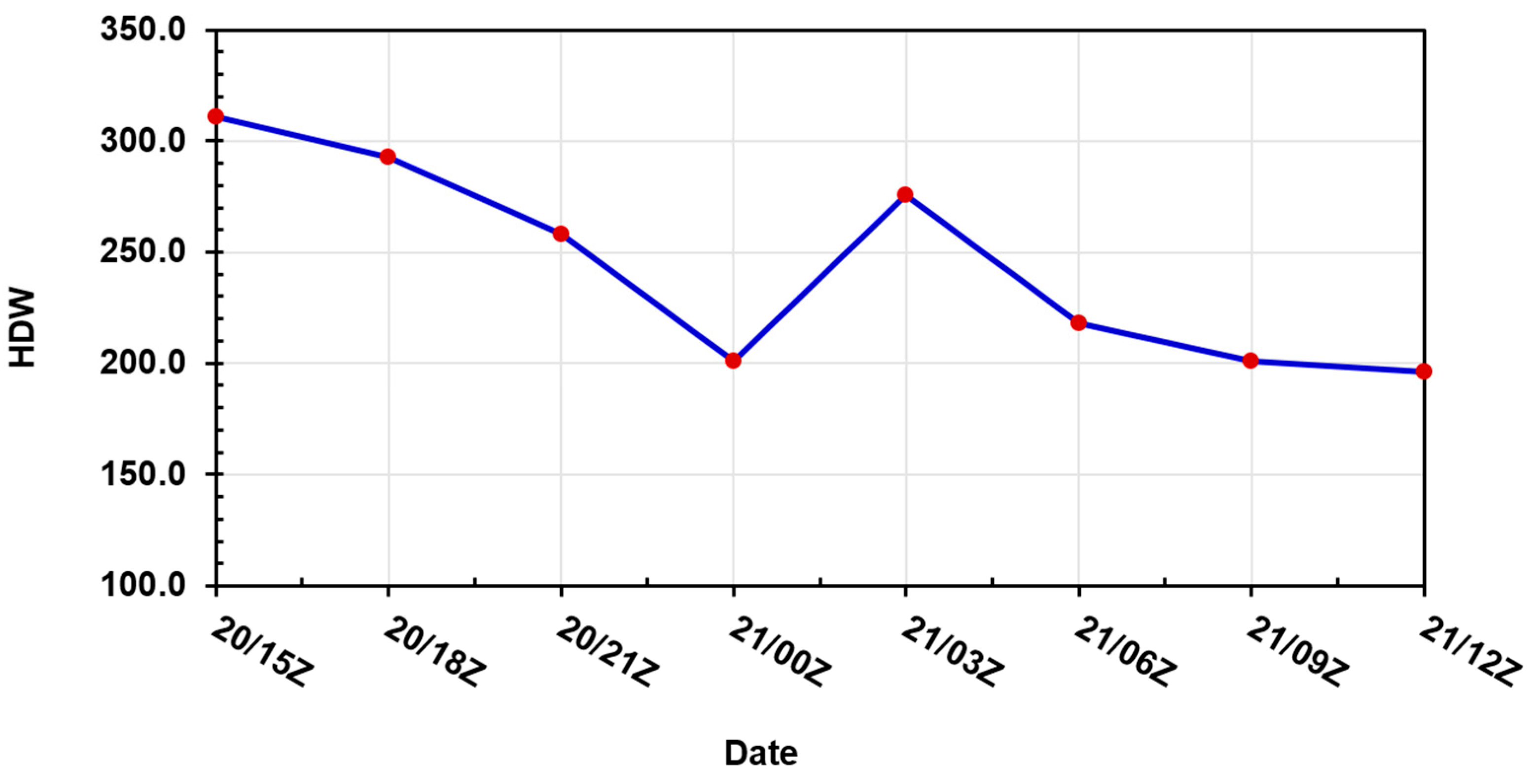
The mesoscale analysis from the WRF simulation shows that the atmosphere was windy, dry, and hot, which are some of the key meteorological variables needed for wildfires to occur [26]. To diagnose more details about the meso-α scale weather activity that caused the East Bay Hills Fire (1991), we calculate the HDW (explained in section 1) using the WRF simulation (4km resolution - d02). For the East Bay Hills Fire event, the WRF simulation results show that the high HDW index is located between the surface and 800m level. Due to this, we selected the highest wind speed and vapor pressure deficit (VPD) from any level in the lowest 800m to the surface, unlike Srock et al. [7], who used the layer from the lowest 500m to the surface. We calculated HDW using our WRF simulated results by following the same approach Srock et al. [7] used in calculating their HDW. In Figure 17, the HDW is shown a few hours before the fire started through the time it abated. On 10/20/15Z, the highest HDW occurred at the fire location (black shaded circle). This high HDW set the pace for favorable wildfire conditions, which started around 10:40 PDT (1740 UTC) on October 20, 1991. At the southeastern and especially southwestern part of the fire location, there is high HDW, and this indicates how the fire moved and affected areas like Berkeley (west), Oakland City (east), Piedmont (southeast), and other nearby cities. In addition, the high HDW at the southwestern part of the fire location shows the winds were predominantly northeasterly, which moved the fire to the southwest of the fire location. Afterward, HDW decreased with time at the fire location until 17:00 PDT on October 20 (0000 UTC October 21). At 20:00 PDT October 20 (0003 UTC October 21), the HDW increased again, most likely due to daytime heating. Afterward, the HDW decreased again up to the end of the simulation period (Figure 18).
6. Concluding Remarks
This study tried to understand the basic atmospheric mechanisms responsible for the East Bay Hills fire (1991) in Oakland, California. In doing so, we examined the conceptual model proposed by the National Weather Service (https://en.wikipedia.org/wiki/Diablo_wind), which explained how the Diablo wind formed and produced the wildfire in northern California. We analyzed observational data using NARR reanalysis datasets and numerical simulations using the WRF model.
Based on our analyses of observed and numerical simulated data, we found a strong upper-level ridge along the West Coast, which induced warm temperatures and dry weather conditions over northern California on October 19 and 20, 1991. Sinking air related to the high pressure decreased the marine air layer thickness, leading to drier and warmer air along the coastal areas. On the other hand, the increasing temperatures induced low MSLP along the coast and produced a strong north-to-northeast pressure gradient across northern California. The strong pressure gradient was evidenced by the pressure difference increasing from 6 to 14 hPa between the San Francisco Bay area and northern Nevada during 10/19/00Z and 10/20/12Z. The strong pressure gradient forced northeasterly winds to accelerate toward the coastal mountain ranges in northern California. Also, cold air advection over the Great Basin supported sinking air motion over the lee side of Sierra Nevada.
We also analyzed whether the local downward motion was directly coupled with the sinking air motion associated with an upper-level jet streak. We tested this issue using the NOAA HYSPLIT model's backward trajectory code. The results indicate that the source of the air parcels that caused the severe winds on the lee side of the East Bay Hills was not directly from the jet streak, considering the minimum parcel pressure of 730 hPa. Instead, the jet streak's right exit region indirectly enhanced downward motion at the lee side of the Sierra Nevada by establishing a favorably discontinuous vertical atmospheric structure above the Sierra Nevada. This structure favored mountain wave amplification and downslope wind formation. The wave-induced descending Sierran Nevada lee side air dried, warmed, and interacted with warm air in the Central Valley. This ensemble airmass of dry and warm air was advected downstream. It generated severe downslope winds at the East Bay Hills' lee side, created hydraulic jump features, and caused wildfire in the East Bay Hills area of northern California. Our further investigation was done using a vertical cross-section of the WRF simulation. The results show that the jet streak's sinking motion was far from the fire location and might not directly influence the East Bay Hills' Lee side's downward motion.
Also, we investigated whether the downward motion at the East Bay Hills area is produced by the resonant amplification mechanism [11] (CP84) followed by Smith's hydraulic jump mechanism [12] (S85), as proposed by Lin [24]. The results verified that the resonant amplification – hydraulic jump mechanism produces severe downslope wind over the East Bay Hills' lee slopes, leading to hot, dry, and windy air, which was conducive to the formation of the East Bay Hills Fire.
Furthermore, we explored the hot, dry, and windy air from the lee side of Sierra Nevada over the Central Valley, which maintains its features. We used temperature, relative humidity (RH), and isotach plots for the analysis. The analysis showed that the hot, dry, and windy air coming from the lee side of Sierra Nevada maintained its characteristics over the Central Valley and intensified when it passed over the lee side of the East Bay Hills.
Finally, we used the HDW index approach Srock et al. [7] proposed to examine the East Bay Hills Fire event predictability. The HDW was used to identify how hot, dry, and windy the environment was during the East Bay Hills Fire (1991). From our results, the highest HDW occurred on 10/20/15Z. It is assumed that the high HDW created favorable weather conditions, which enhanced the potential for rapid and significant area fire spread on 10/20/18Z. After 10/20/18Z, the HDW decreased with time at the fire location until 10/21/03Z. The HDW increased again due to daytime heating. Afterward, the HDW dropped to the end of the simulation, coinciding with the fire abating time.
In addition to the above findings, complex terrain and canyons may have impacted the East Bay Hills Fire event. Further studies are needed to analyze canyons and complex terrain's sensitivity, which will help understand atmospheric mechanisms that affected the East Bay Hills Fire. This can be accomplished in part by conducting a series of idealized large eddy simulations (LES) with the WRF model, possibly in conjunction with an enhanced canyon-scale observational network.
Author Contributions
Dr. W. Agyakwah contributed to writing, computation, and visualization. Dr. Y.-L. Lin and Dr. M. Kaplan contributed to the conceptualization and funding acquisition.
Funding
This research was supported by the National Science Foundation Award AGS-1265783 and the National Center for Atmospheric Research (NCAR) Diversity Fund.
Data Availability Statement
Data processed and used can be available upon request.
Acknowledgments
This research is supported by the NSF Awards 1900621 and 2022961. The authors acknowledge NCAR CISL for supporting computing time on the Cheyenne supercomputer. The insightful discussions and comments on this paper by Drs. J. Zhang, A. Mekonnen, and L. Liu at North Carolina A&T State University are highly appreciated.
Conflicts of Interest
The authors declare no conflicts of interest.
Appendix A
Further figures provide insights into the transport of strong winds over the lee slope of the Sierra Nevada toward the East Bay Hills, using data collected on the meso-β-scale airflow characteristics over the San Francisco Bay Area, which are mainly influenced by the fire.
Figure A1.
Vertical cross-section from the WRF (d03) simulation of Isotachs (shaded; ms-1), isentropes (contour lines; K), and wind barbs from 10/20/15Z to 10/21/06Z. The cross-section is along line CD (denoted in Figure 14).
Figure A1.
Vertical cross-section from the WRF (d03) simulation of Isotachs (shaded; ms-1), isentropes (contour lines; K), and wind barbs from 10/20/15Z to 10/21/06Z. The cross-section is along line CD (denoted in Figure 14).
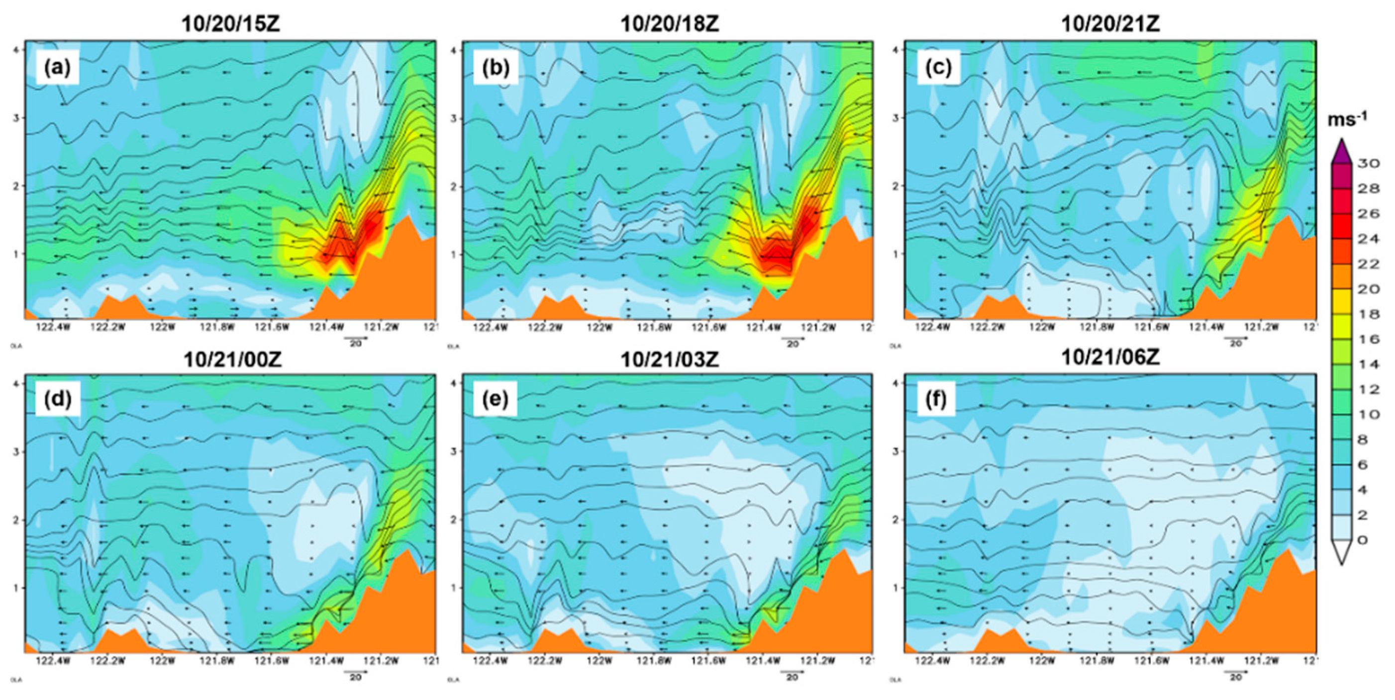
Figure A2.
Vertical cross-section from the WRF (d03) simulation of temperature (shaded; oC), isentropes (contour lines; K), and wind barbs from 10/20/15Z to 10/21/06Z. The cross-section is along line CD (denoted in Figure 14).
Figure A2.
Vertical cross-section from the WRF (d03) simulation of temperature (shaded; oC), isentropes (contour lines; K), and wind barbs from 10/20/15Z to 10/21/06Z. The cross-section is along line CD (denoted in Figure 14).
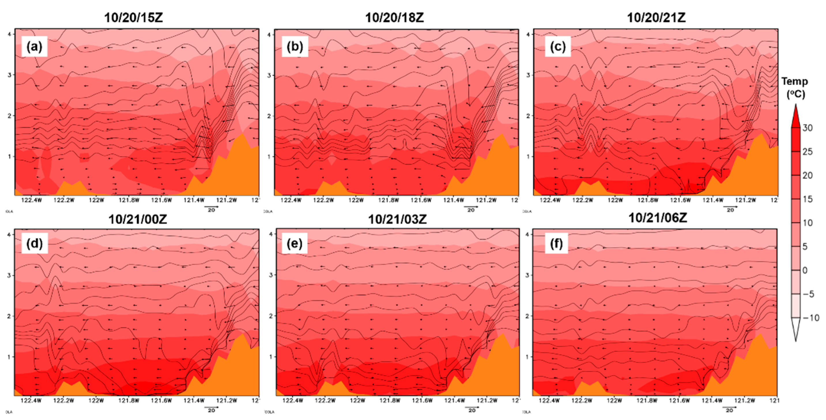
Figure A3.
Vertical cross-section from the WRF (d03) simulation of RH (shaded; %), isentropes (contour lines; K), and wind barbs from 10/20/15Z to 10/21/06Z. The cross-section is along line CD (denoted in Figure 14).
Figure A3.
Vertical cross-section from the WRF (d03) simulation of RH (shaded; %), isentropes (contour lines; K), and wind barbs from 10/20/15Z to 10/21/06Z. The cross-section is along line CD (denoted in Figure 14).

References
- Huang, C.; Lin, Y.-L.; Kaplan, M.L.; Charney, J.J. Synoptic-scale and mesoscale environments conducive to forest fires during the October 2003 extreme fire event in southern California. J. Appl. Meteorol. Climatol. 2009, 48, 553–579. [Google Scholar] [CrossRef]
- Smith, C.M.; Hatchett, B.J.; Kaplan, M.L. Characteristics of Sundowner winds near Santa Barbara, California, from a dynamically downscaled climatology: Environment and effects near the surface. J. Appl. Meteorol. Climatol. 2018, 57, 589–606. [Google Scholar] [CrossRef]
- Kaplan, M.L.; Tilley, J.S.; Hatchett, B.J.; Smith, C.M.; Walston, J.M.; Shourd, K.N.; Lewis, J.M. The Record Los Angeles Heat Event of September 2010: 1. Synoptic-Scale-Meso-β-Scale Analyses of Interactive Planetary Wave Breaking, Terrain- and Coastal-Induced Circulations. J. Geophys. Res. Atmos. 2017, 122, 10–729. [Google Scholar] [CrossRef]
- Sharples, J.J. An overview of mountain meteorological effects relevant to fire behavior and bushfire risk. Int. J. Wildland Fire 2009, 18, 737–754. [Google Scholar] [CrossRef]
- Smith, C.; Hatchett, B.J.; Kaplan, M. A surface observation-based climatology of Diablo-like winds in California's wine country and western Sierra Nevada. Fire 2018, 1, 25. [Google Scholar] [CrossRef]
- Routley, J.G. East Bay Hills fire Oakland-Berkeley, California. Emmitsburg, MD: United States Fire Administration 1991.
- Srock, A.F.; Charney, J.J.; Potter, B.E.; Goodrick, S.L. The hot-dry-windy index: A new fire weather index. Atmosphere 2018, 9, 279. [Google Scholar] [CrossRef]
- Simard, A.J.; Haines, D.A.; Blank, R.W.; Frost, J.S. The Mack Lake fire. General Technical Report NC-83. St. Paul, MN: US Dept. of Agriculture, Forest Service, North Central Forest Experiment Station 1983, 83.
- Haines, D.A. A lower atmospheric severity index for wildland fire. Natl. Weather Dig. 1988, 13, 23–27. [Google Scholar]
- Pechony, O.; Shindell, D.T. Fire parameterization on a global scale. J. Geophys. Res. Atmos. 2009, 114, D16. [Google Scholar] [CrossRef]
- Clark, T.L.; Peltier, W.R. Critical level reflection and the resonant growth of nonlinear mountain waves. J. Atmos. Sci. 1984, 41, 3122–3134. [Google Scholar] [CrossRef]
- Smith, R.B. On severe downslope winds. J. Atmos. Sci. 1985, 42, 2597–2603. [Google Scholar] [CrossRef]
- Lin, Y.-L.; Wang, T.A. Flow regimes and transient dynamics of two-dimensional stratified flow over an isolated mountain ridge. J. Atmos. Sci. 1996, 53, 139–158. [Google Scholar] [CrossRef]
- Skamarock, W.C.; Klemp, J.B.; Dudhia, J.; Gill, D.O.; Barker, D.; Duda, M.G.; Huang, X.-Y.; Wang, W.; Powers, J.G. A Description of the Advanced Research WRF Version 3. University Corporation for Atmospheric Research 2008. [Google Scholar] [CrossRef]
- Lin, Y.-L.; Farley, R.D.; Orville, H.D. Bulk parameterization of the snow field in a cloud model. J. Appl. Meteorol. Climatol. 1983, 22, 1065–1092. [Google Scholar] [CrossRef]
- Kain, J.S. The Kain-Fritsch convective parameterization: An update. J. Appl. Meteorol. 2004, 43, 170–181. [Google Scholar] [CrossRef]
- Janjic, Z.I. The step-mountain Eta coordinate model: Further developments of the convection, viscous layer, and turbulence closure schemes. Mon. Weather Rev. 1994, 122, 927–945. [Google Scholar] [CrossRef]
- Mlawer, E.J.; Taubman, S.J.; Brown, P.D.; Iacono, M.J.; Clough, S.A. Radiative transfer for inhomogeneous atmospheres: RRTM, a validated correlated-k model for the longwave. J. Geophys. Res. Atmos. 1997, 102, 16663–16682. [Google Scholar] [CrossRef]
- Iacono, M.J.; Delamere, J.S.; Mlawer, E.J.; Shephard, M.W.; Clough, S.A.; Collins, W.D. Radiative forcing by long-lived greenhouse gases: Calculations with the AER radiative transfer models. J. Geophys. Res. Atmos. 2008, 113, D13. [Google Scholar] [CrossRef]
- US Department of Commerce, NOAA, NWS. The marine layer. NWS JetStream 2019. https://www.noaa.gov/jetstream/ocean/marine-layer.
- National Oceanic and Atmospheric Administration (NOAA). "Tunnel" wildfire Oakland-Berkeley hills October 20–23, 1991. Natural Disaster Survey Report. US Department of Commerce, NOAA, NWS 1992.
- Uccellini, L.W.; Johnson, D.R. The Coupling of Upper and Lower Tropospheric Jet Streaks and Implications for the Development of Severe Convective Storms. Mon. Weather Rev. 1979, 107, 682–703. [Google Scholar] [CrossRef]
- Uccellini, L.W.; Kocin, P.J. The interaction of jet streak circulations during heavy snow events along the east coast of the United States. Weather Forecasting 1987, 2, 289–308. [Google Scholar] [CrossRef]
- Lin, Y.-L. Mesoscale Dynamics; Cambridge University Press: Cambridge, UK, 2007. [Google Scholar] [CrossRef]
- Scinocca, J.F.; Peltier, W.R. The instability of Long's stationary solution and the evolution toward severe downslope windstorm flow. Part I: Nested grid numerical simulations. J. Atmos. Sci. 1993, 50, 2245–2263. [Google Scholar] [CrossRef]
- Erickson, M.J.; Charney, J.J.; Colle, B.A. Development of a Fire Weather Index Using Meteorological Observations within the Northeast United States. J. Appl. Meteorol. Climatol. 2016, 55, 389–402. [Google Scholar] [CrossRef]
Figure 1.
Domain set up for the East Bay Hills Fire (1991) with three nested domains with grid resolutions of 16km (d01), 4km (d02), and 1km (d03). On the left-hand side is the zoomed-in of the San Francisco Bay area and the East Bay Hills Fire location.
Figure 1.
Domain set up for the East Bay Hills Fire (1991) with three nested domains with grid resolutions of 16km (d01), 4km (d02), and 1km (d03). On the left-hand side is the zoomed-in of the San Francisco Bay area and the East Bay Hills Fire location.
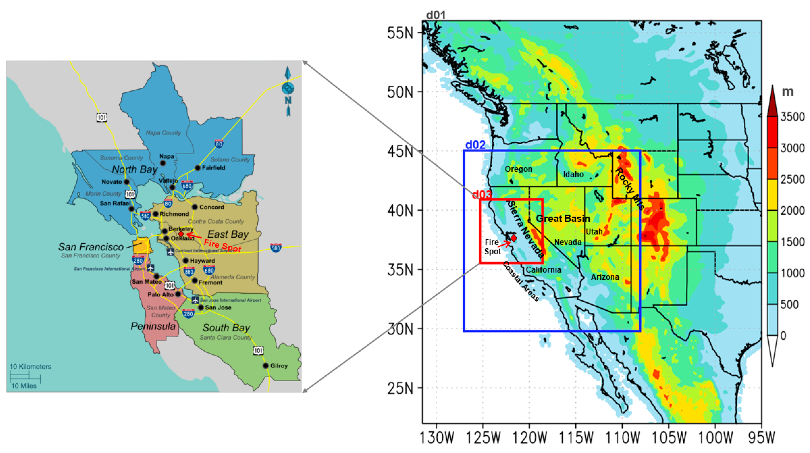
Figure 2.
North American Regional Reanalysis (NARR) data of 500 hPa geopotential height (shaded) and wind barbs valid at (a) 10/19/00Z, (b) 10/19/12Z, (c) 10/20/00Z, and (d) 10/20/12Z. NNV indicates northern Nevada, and SFB is San Francisco Bay.
Figure 2.
North American Regional Reanalysis (NARR) data of 500 hPa geopotential height (shaded) and wind barbs valid at (a) 10/19/00Z, (b) 10/19/12Z, (c) 10/20/00Z, and (d) 10/20/12Z. NNV indicates northern Nevada, and SFB is San Francisco Bay.
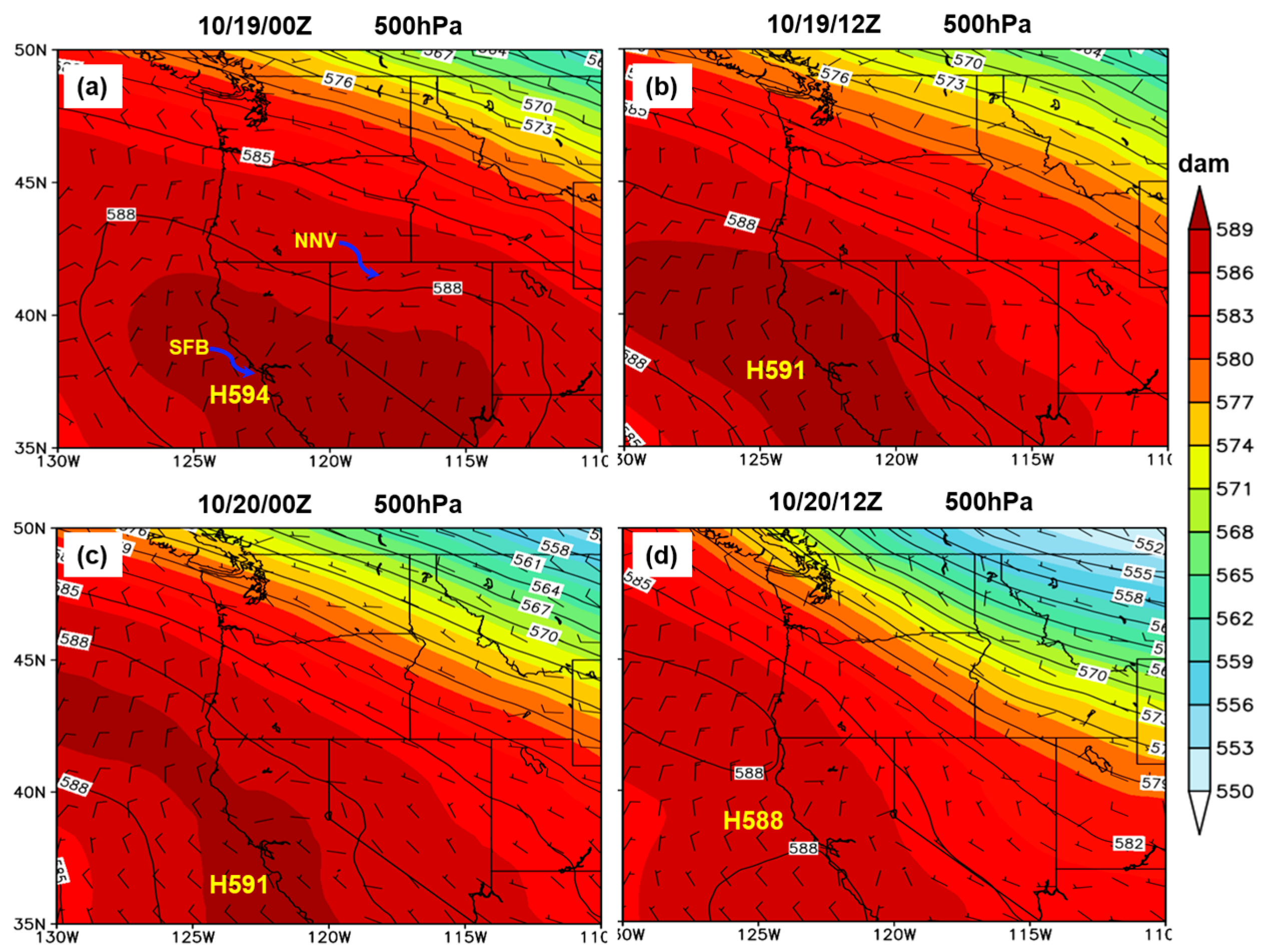
Figure 3.
North American Regional Reanalysis (NARR) data of MSLP (shaded and contour lines; hPa) and wind barbs at (a) 10/19/00Z, (b) 10/19/12Z, (c) 10/20/00Z, and (d) 10/20/12Z. NNV indicates northern Nevada, and SFB is San Francisco Bay.
Figure 3.
North American Regional Reanalysis (NARR) data of MSLP (shaded and contour lines; hPa) and wind barbs at (a) 10/19/00Z, (b) 10/19/12Z, (c) 10/20/00Z, and (d) 10/20/12Z. NNV indicates northern Nevada, and SFB is San Francisco Bay.
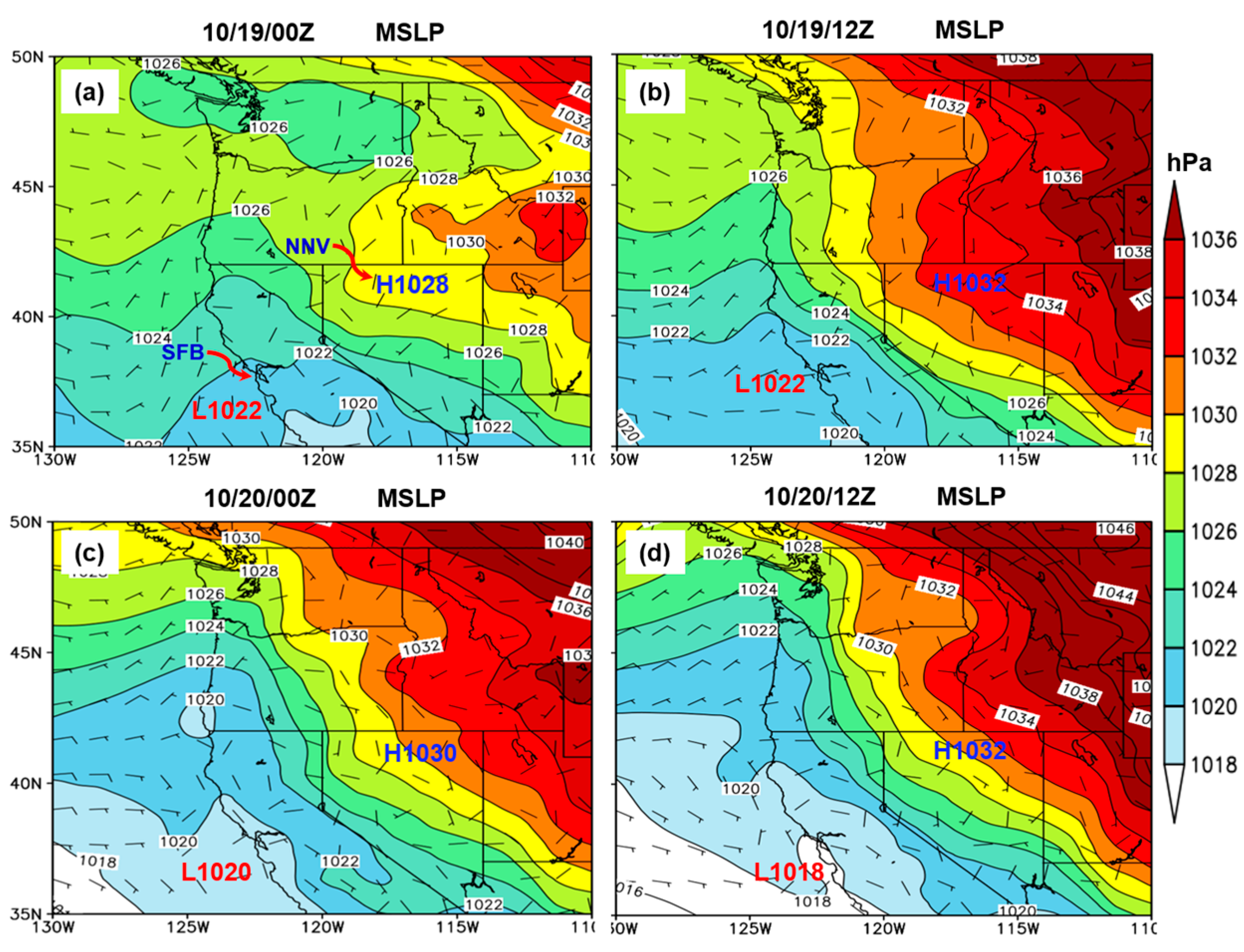
Figure 4.
Observed thermodynamic diagram for Oakland International Airport valid at (a) 1200 UTC Oct 19, (b) 0000 UTC Oct 20, (c) 1200 UTC Oct 20, (d) 0000 UTC Oct 21 and (e) 1200 UTC Oct 21 and (f) 0000 UTC Oct 22. The solid line on the left denotes dewpoint temperature, and on the right is temperature.
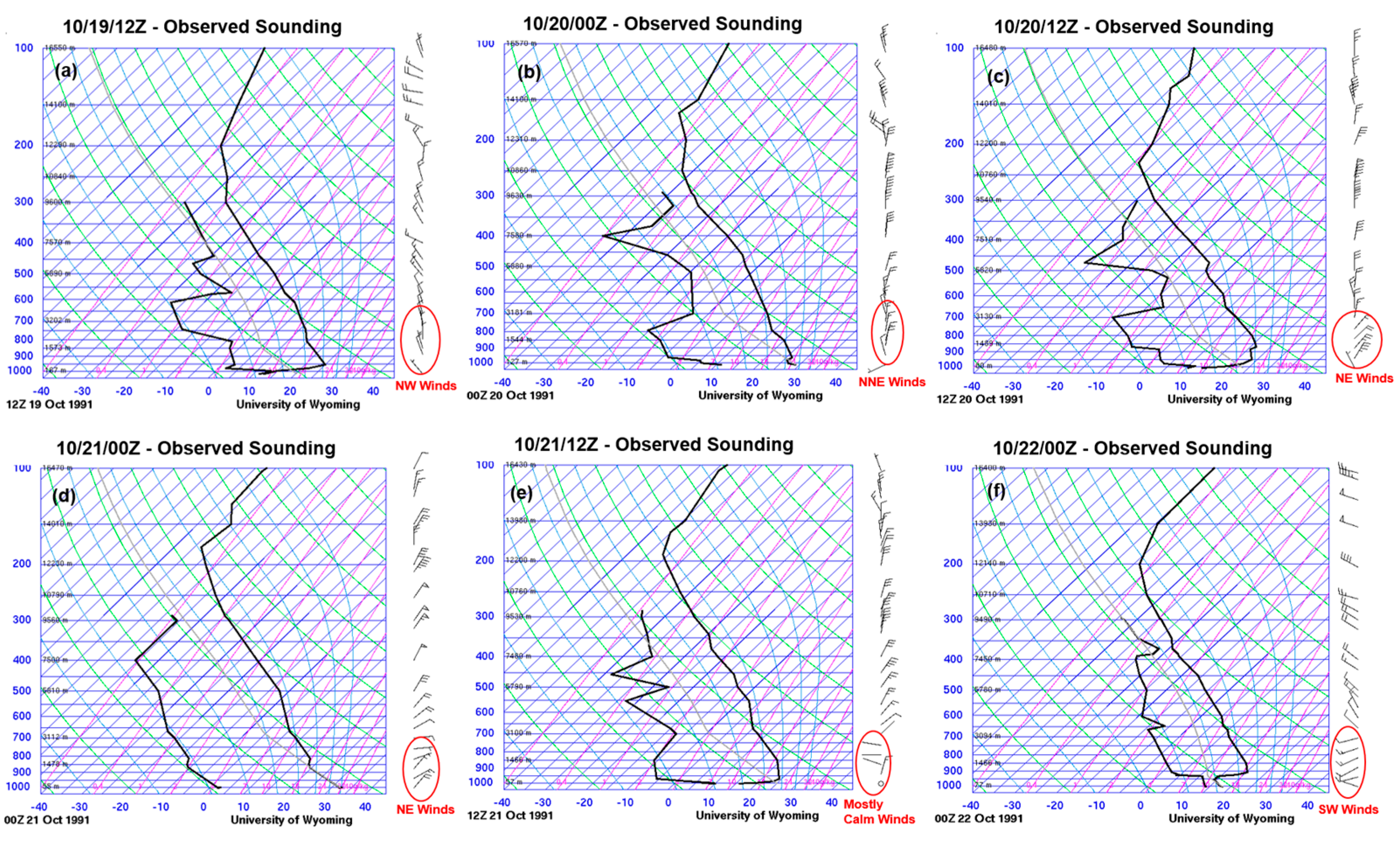
Figure 5.
WRF (d02) simulation of isotachs (shaded; ms-1) and wind barbs at (a),(b) 250 hPa, (c),(d) 700 hPa, (e),(f) 850 hPa and (g),(h) 10m above ground level at (left) 1500 UTC Oct 20 and (right) 1800 UTC Oct 20.
Figure 5.
WRF (d02) simulation of isotachs (shaded; ms-1) and wind barbs at (a),(b) 250 hPa, (c),(d) 700 hPa, (e),(f) 850 hPa and (g),(h) 10m above ground level at (left) 1500 UTC Oct 20 and (right) 1800 UTC Oct 20.
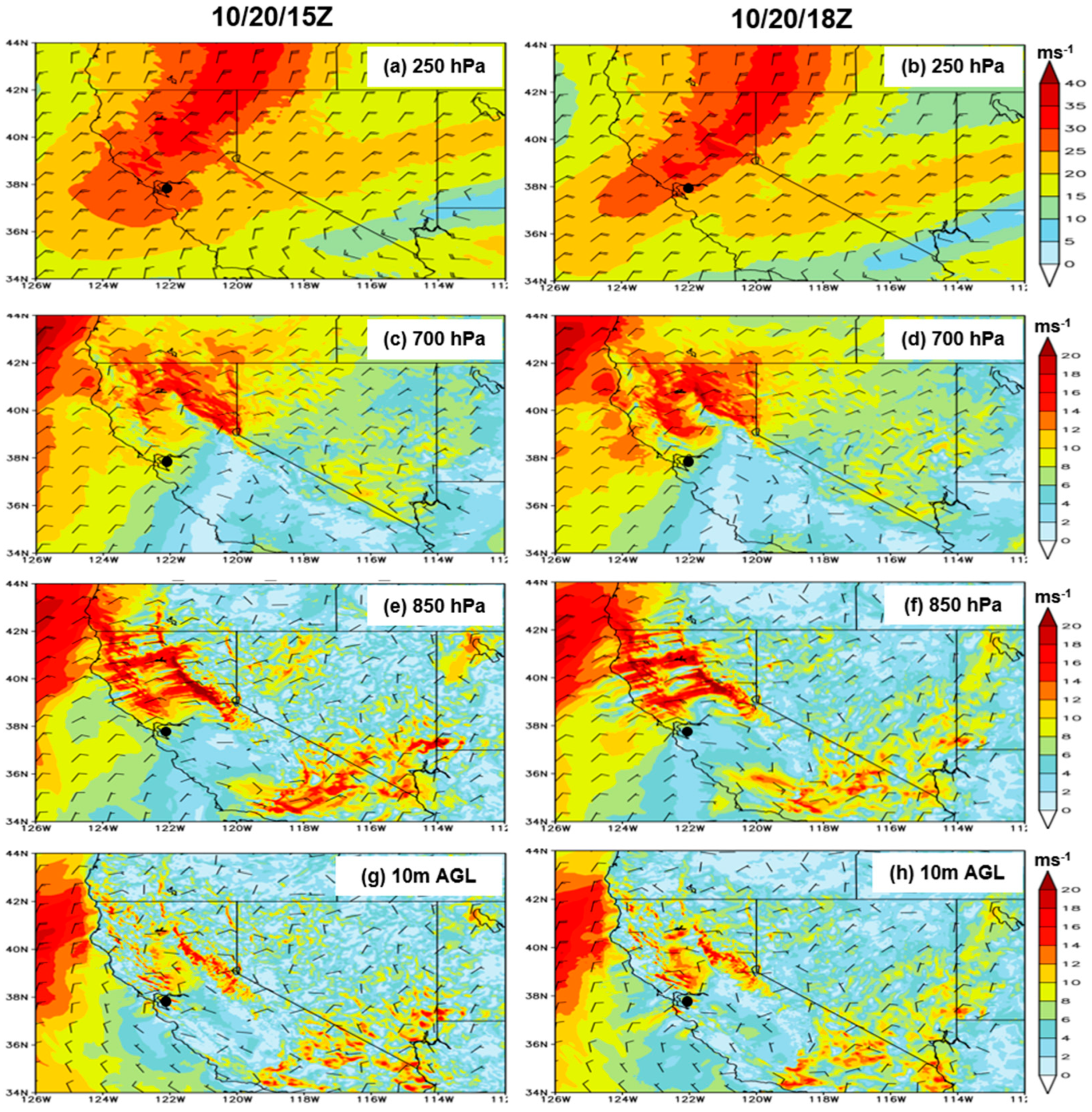
Figure 6.
WRF (d02) simulation of isotachs (shaded; ms-1) and wind barbs of (a),(b) 250 hPa, (c),(d) 700 hPa, (e),(f) 850 hPa and (g),(h) 10m above ground level at (left) 0600 UTC Oct 21 and (right) 1200 UTC Oct 21.
Figure 6.
WRF (d02) simulation of isotachs (shaded; ms-1) and wind barbs of (a),(b) 250 hPa, (c),(d) 700 hPa, (e),(f) 850 hPa and (g),(h) 10m above ground level at (left) 0600 UTC Oct 21 and (right) 1200 UTC Oct 21.
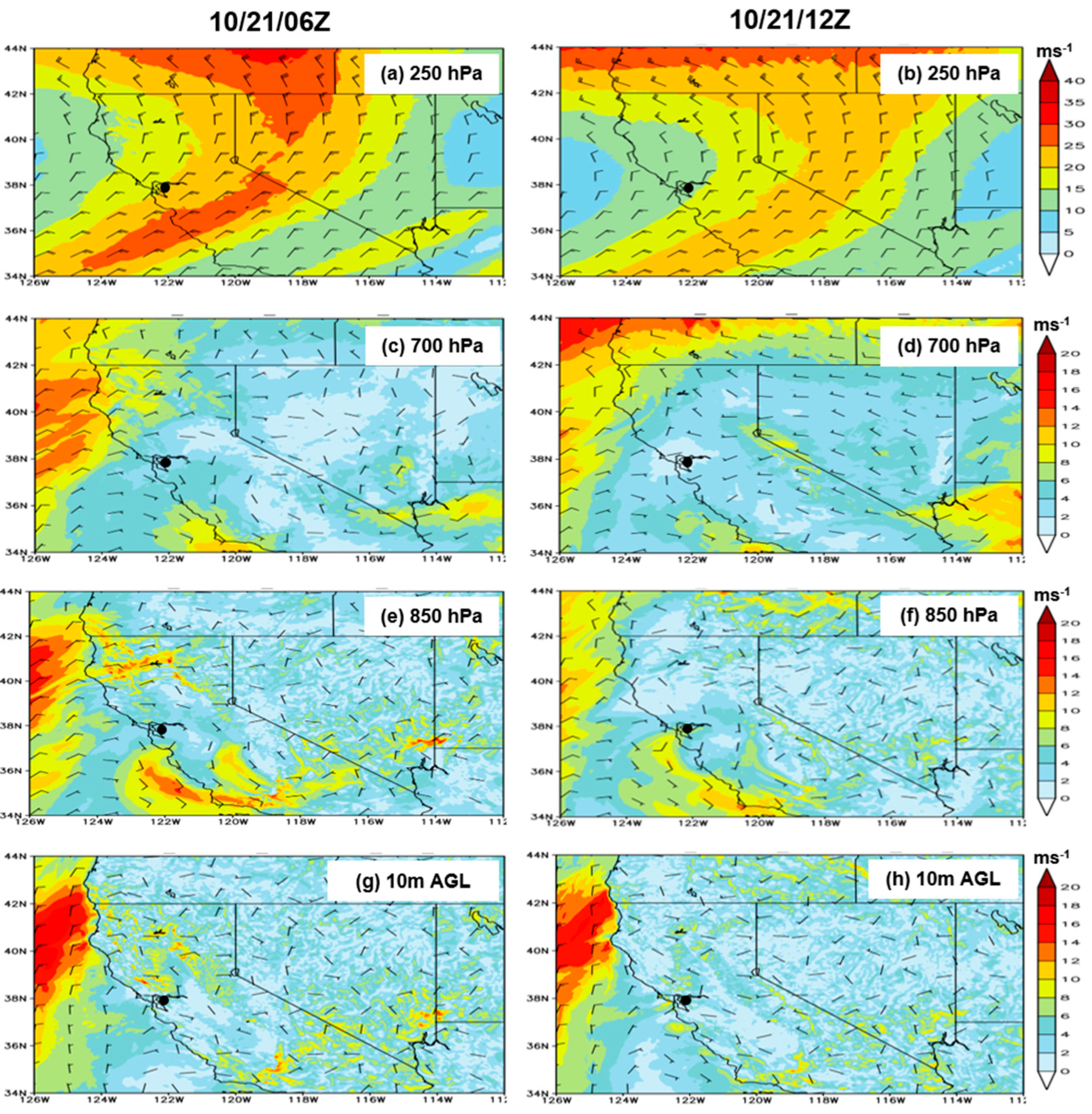
Figure 7.
WRF (d02) simulation of RH (shaded; %) and wind barbs of (a),(b) 250 hPa, (c),(d) 700 hPa, (e),(f) 850 hPa, and (g),(h) 10m above ground level at (left) 1500 UTC Oct 20 and (right) 1800 UTC Oct 20.
Figure 7.
WRF (d02) simulation of RH (shaded; %) and wind barbs of (a),(b) 250 hPa, (c),(d) 700 hPa, (e),(f) 850 hPa, and (g),(h) 10m above ground level at (left) 1500 UTC Oct 20 and (right) 1800 UTC Oct 20.
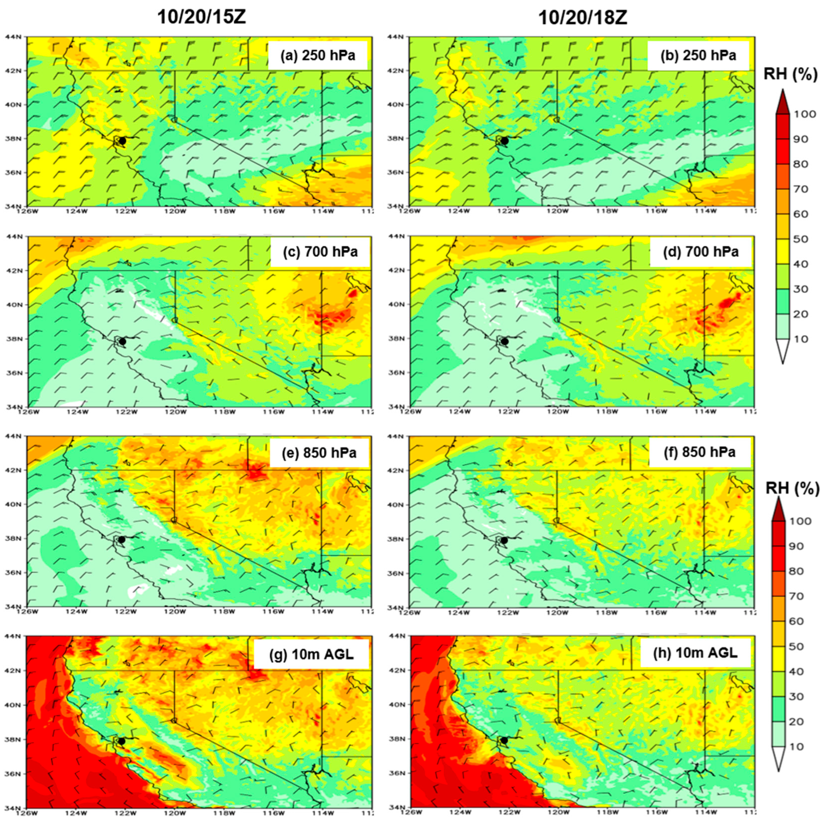
Figure 8.
WRF (d02) simulation of RH (shaded; %) and wind barbs of (a),(b) 250 hPa, (c),(d) 700 hPa, (e),(f) 850 hPa, and (g),(h) 10m above ground level at (left) 0600 UTC Oct 21 and (right) 1200 UTC Oct 21.
Figure 8.
WRF (d02) simulation of RH (shaded; %) and wind barbs of (a),(b) 250 hPa, (c),(d) 700 hPa, (e),(f) 850 hPa, and (g),(h) 10m above ground level at (left) 0600 UTC Oct 21 and (right) 1200 UTC Oct 21.

Figure 9.
WRF (d02) simulation of temperature (shaded; oC) and wind barbs of (a),(b) 250 hPa, (c),(d) 700 hPa, (e),(f) 850 hPa, and (g),(h) 10m above ground level at (left) 1500 UTC Oct 20 and (right) 1800 UTC Oct 20.
Figure 9.
WRF (d02) simulation of temperature (shaded; oC) and wind barbs of (a),(b) 250 hPa, (c),(d) 700 hPa, (e),(f) 850 hPa, and (g),(h) 10m above ground level at (left) 1500 UTC Oct 20 and (right) 1800 UTC Oct 20.
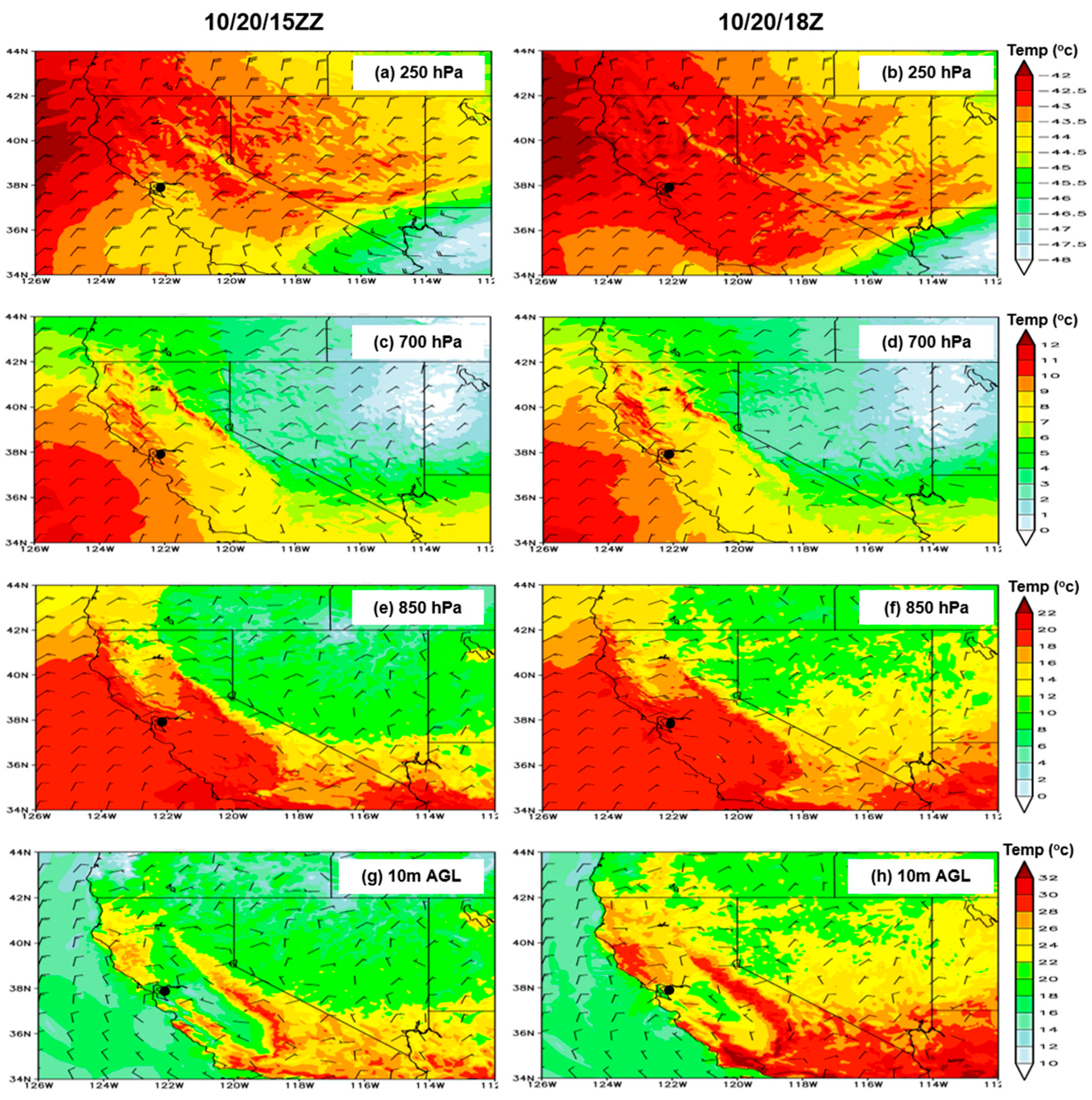
Figure 10.
WRF (d02) simulation of temperature (shaded; oC) and wind barbs of (a),(b) 250 hPa, (c),(d) 700 hPa, (e),(f) 850 hPa, and (g),(h) 10m above ground level at (left) 0600 UTC Oct 21 and (right) 1200 UTC Oct 21.
Figure 10.
WRF (d02) simulation of temperature (shaded; oC) and wind barbs of (a),(b) 250 hPa, (c),(d) 700 hPa, (e),(f) 850 hPa, and (g),(h) 10m above ground level at (left) 0600 UTC Oct 21 and (right) 1200 UTC Oct 21.
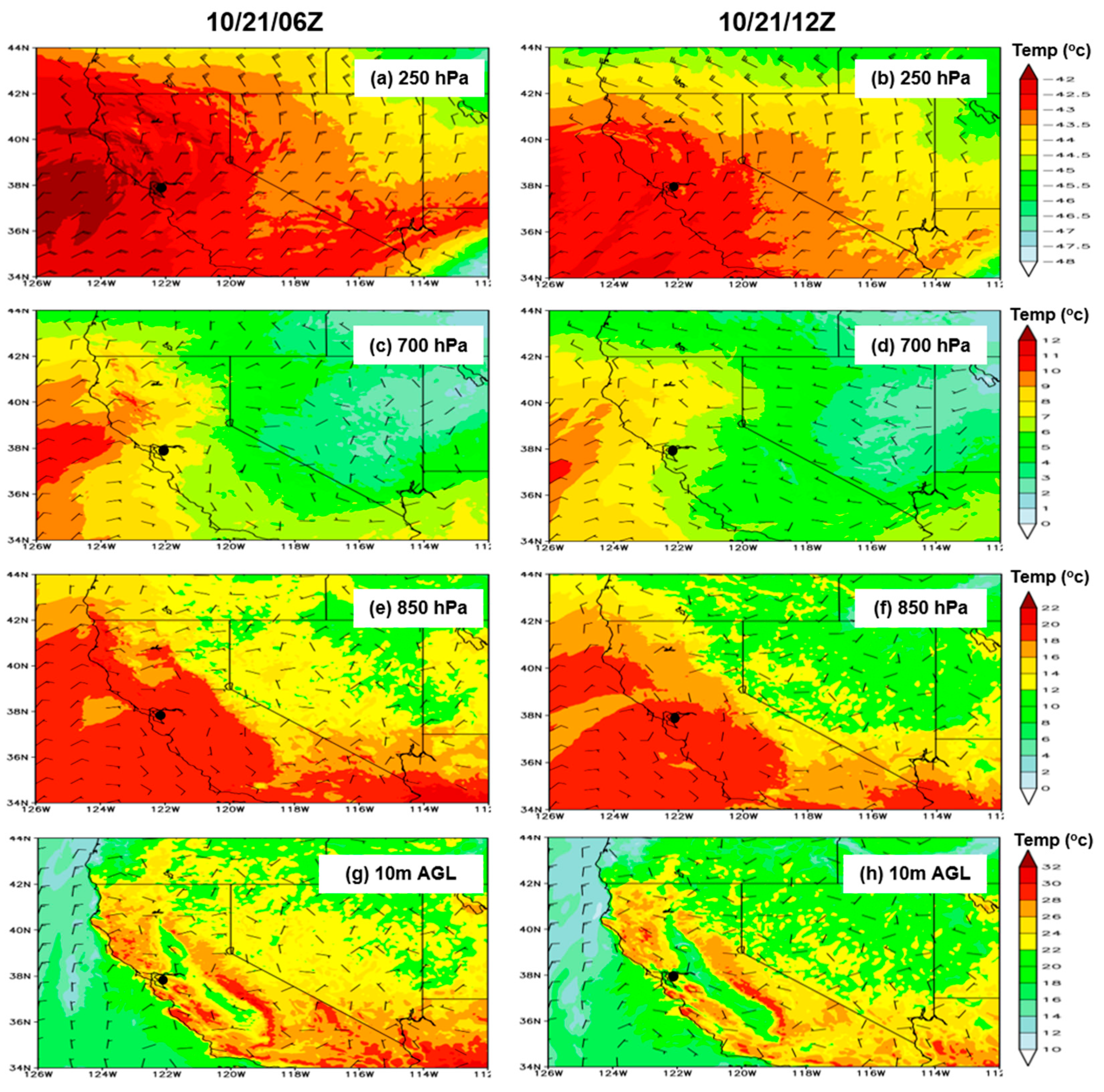
Figure 11.
Backward trajectory analysis of winds from the NARR meteorological data starting from the fire location (37.86oN, 122.22oW) starting at 1500 UTC Oct 20, 1991 (a) and 1800 UTC October 20, 1991 (b). They all end at 1200 UTC Oct 18, 1991. .
Figure 11.
Backward trajectory analysis of winds from the NARR meteorological data starting from the fire location (37.86oN, 122.22oW) starting at 1500 UTC Oct 20, 1991 (a) and 1800 UTC October 20, 1991 (b). They all end at 1200 UTC Oct 18, 1991. .
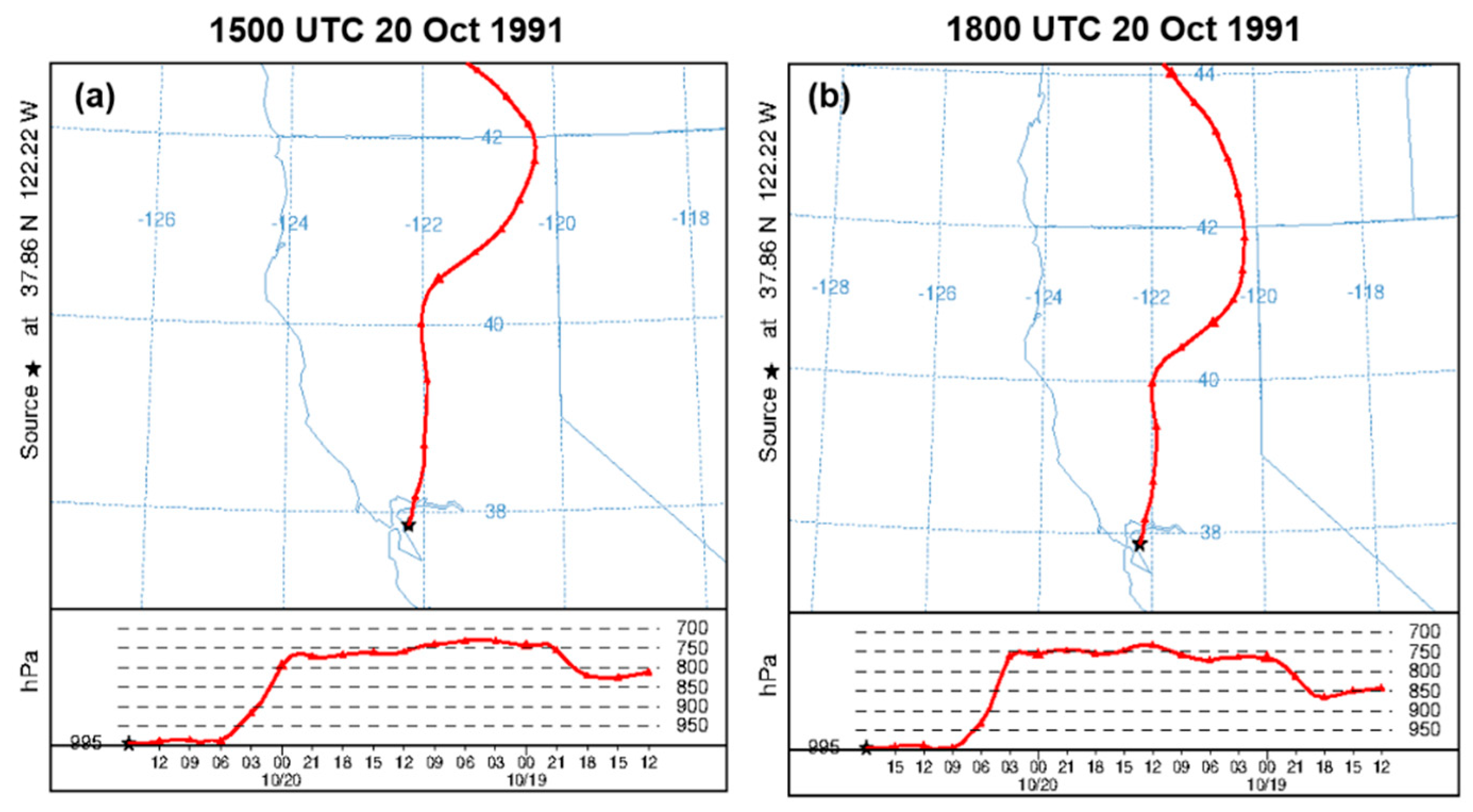
Figure 12.
Cross-section along AB (denoted in the upper-right corner) from the WRF (d01) simulation of isotachs (shaded; ms-1), isentropes (contour lines; K), and wind barbs. The cross-section line passes through the jet streak's right exit region and the fire location at 250 hPa level.
Figure 12.
Cross-section along AB (denoted in the upper-right corner) from the WRF (d01) simulation of isotachs (shaded; ms-1), isentropes (contour lines; K), and wind barbs. The cross-section line passes through the jet streak's right exit region and the fire location at 250 hPa level.
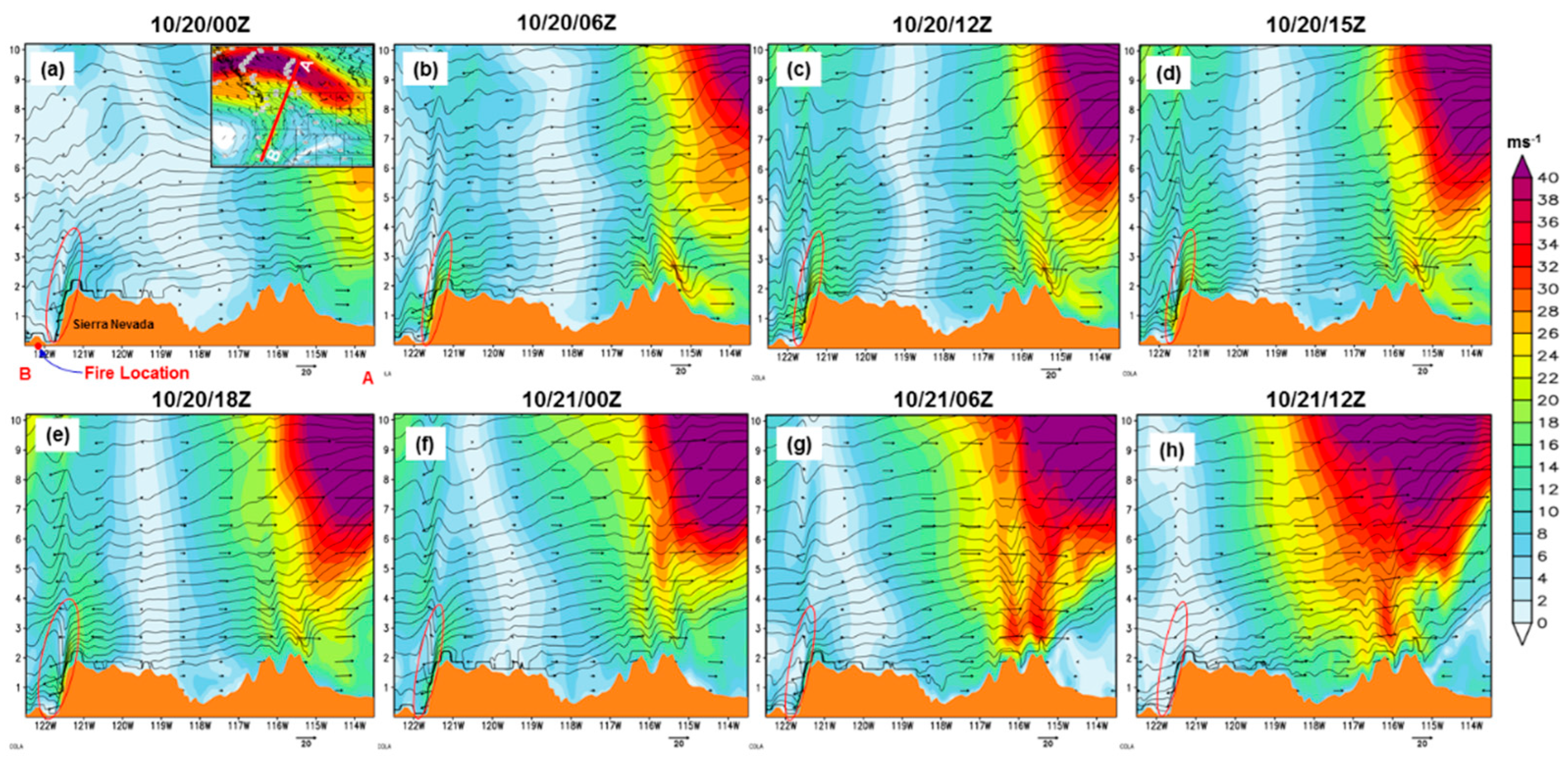
Figure 13.
Vertical cross-section at the lee side of Sierra Nevada using the WRF (d02) simulation of (a) isotachs (shaded; ms-1) and isentropes (contour lines; K), (b) isentropes (shaded; K), and (c) TKE (shaded; m2s-2) and isentropes (contour lines; K) from 10/20/06Z to 10/20/18Z. CL represents a critical level, and HJ means hydraulic jump.
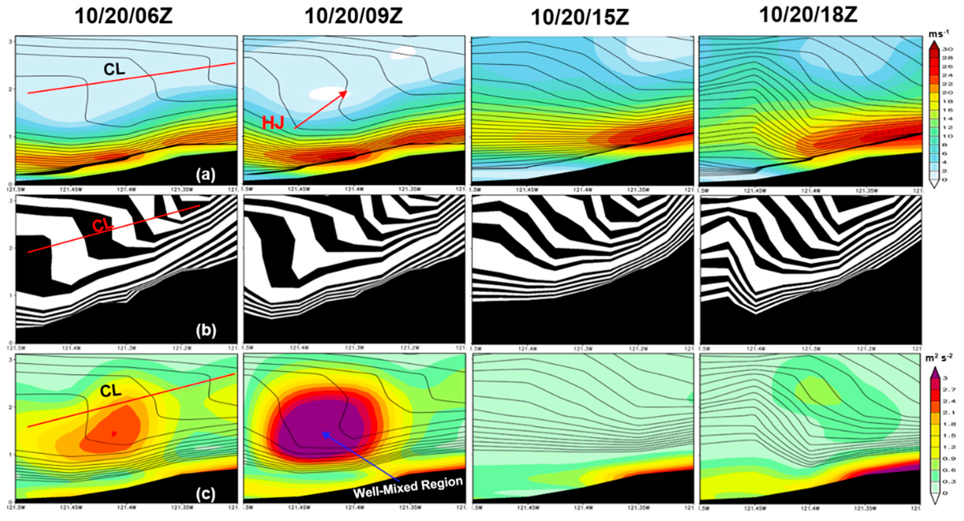
Figure 14.
Cross-section along line CD (indicated in the upper-left panel) from the WRF (d02) simulation of isotachs (shaded; ms-1), isentropes (contour lines; K), and wind barbs. The red dashed lines represent the level where wind reversal occurs. The two horizontal lines are critical level heights calculated using Clark and Peltier's resonant amplification (upper) and Smith's hydraulic mechanisms (upper & lower).
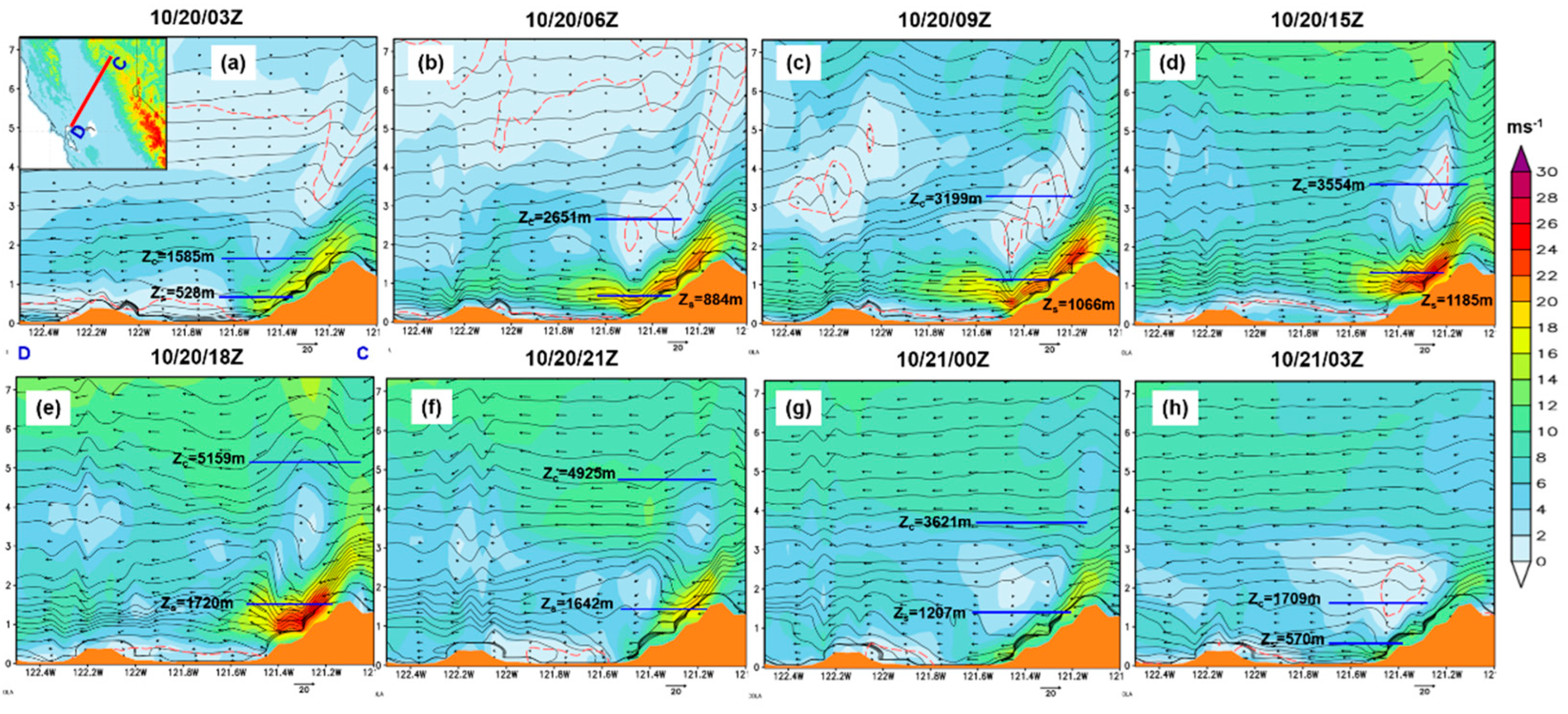
Figure 15.
Cross-section along line CD (denoted in Figure 14) from the WRF (d02) simulation of temperature (shaded; oC), isentropes (contour lines; K), and wind barbs from 10/20/03Z to 10/21/03Z.
Figure 15.
Cross-section along line CD (denoted in Figure 14) from the WRF (d02) simulation of temperature (shaded; oC), isentropes (contour lines; K), and wind barbs from 10/20/03Z to 10/21/03Z.
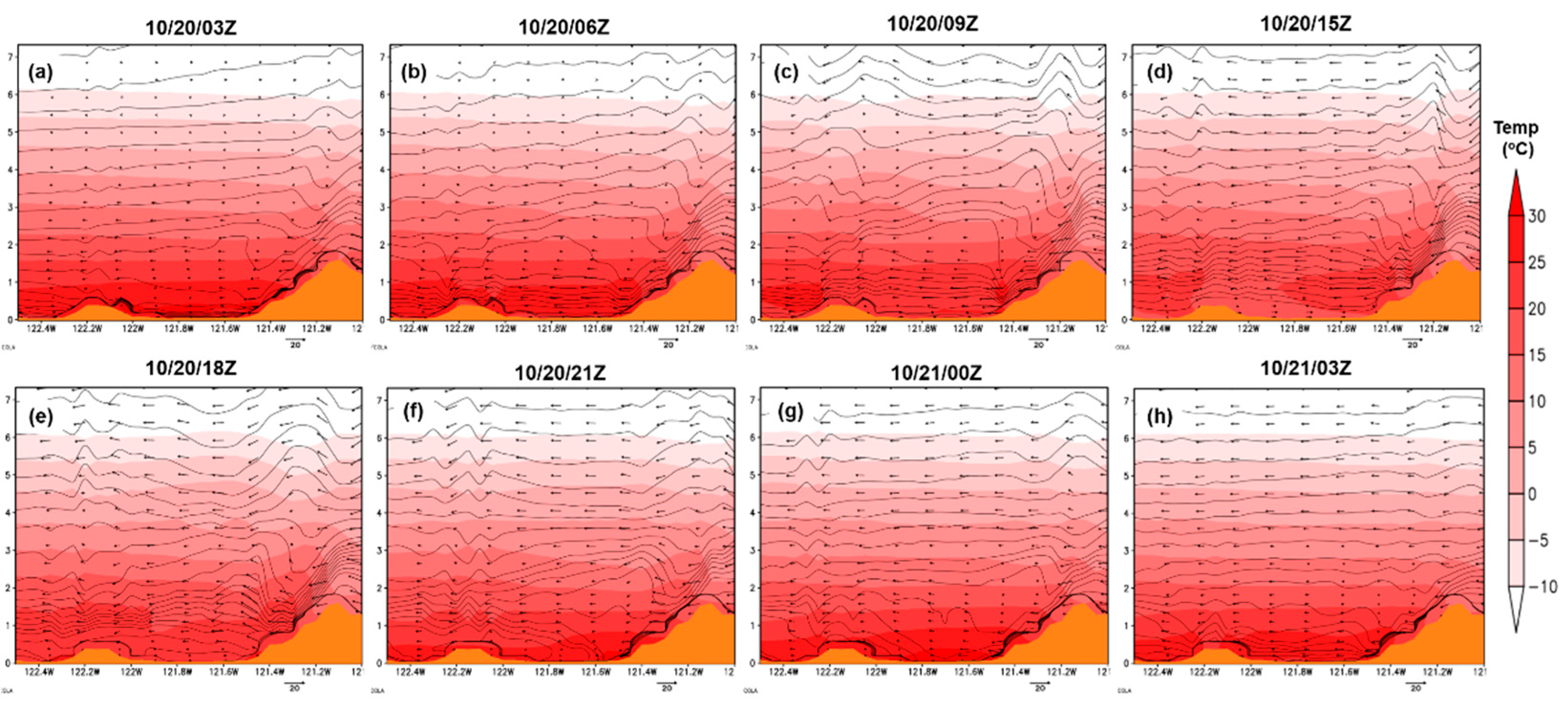
Figure 16.
Cross-section along line CD (denoted in Figure 14) from the WRF (d02) simulation of RH (shaded; %), isentropes (contour lines; K), and wind barbs from 10/20/03Z to 10/21/03Z.
Figure 16.
Cross-section along line CD (denoted in Figure 14) from the WRF (d02) simulation of RH (shaded; %), isentropes (contour lines; K), and wind barbs from 10/20/03Z to 10/21/03Z.
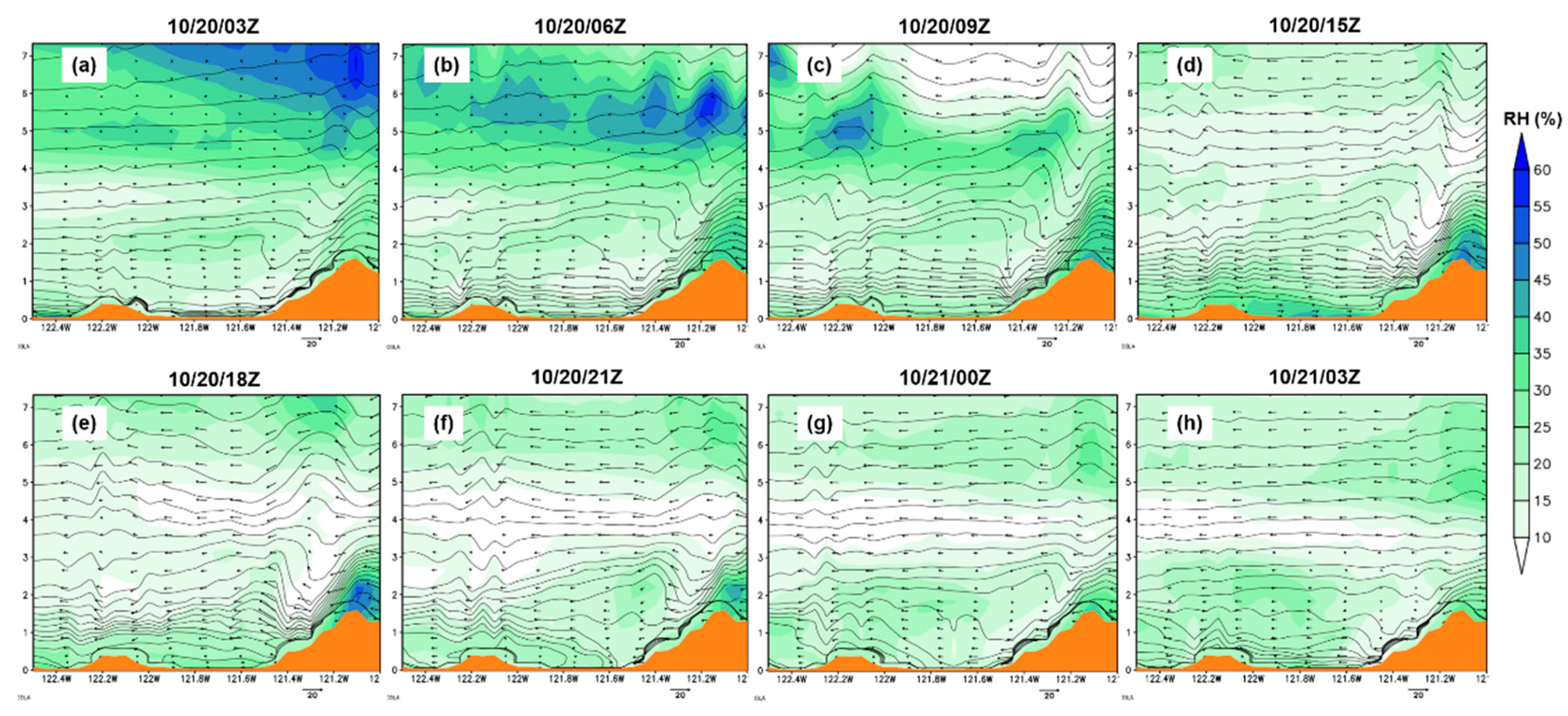
Figure 17.
Maximum HDW (shaded) using WRF (d02) simulated data from 10/20/15Z to 10/21/12Z. The black dot indicates the fire location (37.86 N latitude and 122.22 W longitude). .
Figure 17.
Maximum HDW (shaded) using WRF (d02) simulated data from 10/20/15Z to 10/21/12Z. The black dot indicates the fire location (37.86 N latitude and 122.22 W longitude). .

Figure 18.
Time series of the HDW using WRF (d02) simulated data at the fire location (37.86o N latitude and 122.22o W longitude) from 10/20/15Z to 10/21/12Z.
Figure 18.
Time series of the HDW using WRF (d02) simulated data at the fire location (37.86o N latitude and 122.22o W longitude) from 10/20/15Z to 10/21/12Z.
Disclaimer/Publisher’s Note: The statements, opinions and data contained in all publications are solely those of the individual author(s) and contributor(s) and not of MDPI and/or the editor(s). MDPI and/or the editor(s) disclaim responsibility for any injury to people or property resulting from any ideas, methods, instructions or products referred to in the content. |
© 2024 by the authors. Licensee MDPI, Basel, Switzerland. This article is an open access article distributed under the terms and conditions of the Creative Commons Attribution (CC BY) license (http://creativecommons.org/licenses/by/4.0/).
Copyright: This open access article is published under a Creative Commons CC BY 4.0 license, which permit the free download, distribution, and reuse, provided that the author and preprint are cited in any reuse.


