
Submitted:
16 December 2024
Posted:
17 December 2024
You are already at the latest version
Abstract
Mineral resources and metals are integral to modern society, with growing demand driven by recent technological advancements. Life Cycle Assessment (LCA) provides a valuable framework for assessing resource use, and numerous methodologies have been developed to address both midpoint and endpoint levels of life cycle impact assessment (LCIA). This review aims to provide a comprehensive overview of the existing LCIA methodologies related to minerals and metals, with a focus on recent developments, progress made, and potential future directions. It examines these LCIA methods in terms of resources considered, underlying assumptions, data sources and identified limitations. Particularly, a central focus is placed on Rare Earth Elements (REEs), designated as critical raw materials by the European Union and other regions or governments. These REEs are mainly used in electrical and electronic components (e.g. electric vehicle motors) and in various renewable energy technologies (e.g. wind turbines) due to their unique properties that make them difficult to substitute. However, their supply is constrained by limited global reserves and their concentration in a few countries. This situation highlights the need for more reliable and accurate data on resource production and recycling. Additionally, this review presents case studies that apply LCIA methods to real-world scenarios, illustrating current capabilities as well as areas where further research and refinement are needed.
Keywords:
Life Cycle Assessment
; Life Cycle Impact Assessment
; Resource Depletion
; Minerals
; Metals
; Rare Earth Elements
1. Introduction
Mineral resources have long been fundamental to human society, and their importance continues to grow. Minerals and metals are found in varying quantities on the earth, but all are susceptible to depletion, and their extraction has intensified significantly in recent years. This escalation is partly due to the growing demand for materials essential to emerging technologies related to IT equipment, clean energy (e.g. photovoltaic panels, wind turbines), electric vehicles, semiconductors and batteries. Particular attention must be paid to those raw materials that have been identified as critical by the European Union (EU) and various national governments. For example, a study on critical raw materials for the EU in 2023 [1], resulted in 34 critical resources, while the United States Geological Survey (USGS) published 50 critical minerals in 2022 [2]. Resource criticality is influenced by several factors, including economic and strategic importance, potential supply chain disruption, geopolitical risk and absence of suitable substitutes. Therefore, understanding the Environmental, Social and Governance (ESG) impacts associated with the extraction, processing, and consumption of these resources is a key objective in pursuing the United Nations’ 2030 Agenda and its 17 Sustainable Development Goals (SDGs). Particularly, the mining industry can be directly or indirectly linked to several SDGs, including SDG 6 (Clean Water and Sanitation), SDG 7 (Affordable and Clean Energy), SDG 8 (Work and Economic Growth), SDG 9 (Industry, Innovation and Infrastructure), SDG 11 (Sustainable Cities and Communities), SDG 12 (Responsible Production and Consumption), SDG 13 (Climate Action) and SDG 15 (Life on Land) [3]. As such, the responsible management of mineral resources is crucial to advancing global sustainability objectives.
Life Cycle Assessment (LCA) [4,5] offers a systematic framework to assess the extraction, use and potential environmental impacts of mineral resource extraction across its life cycle. Meanwhile, different methods are used for assessing impacts and their characterization factors (CFs) have been proposed over the past three decades. As reported in Sonderegger et al. [6], such various methods can be broadly grouped into 4 families: “Depletion methods”, “Supply Risk methods”, “Future Effort methods” and “Thermodynamic methods”. Taking inspiration from this classification, this review firstly synthesizes the main life cycle impact assessment (LCIA) methods developed for mineral resource extraction since the early 1990s, focusing on their mathematical formulation, the elements considered and the main limitations. This work is carried out using the Scopus database and building upon prior review studies, pays particular attention to critical materials—specifically, Rare Earth Elements (REEs). The goal of this analysis is to clarify the data requirements necessary for implementing more precise methodologies that can better support LCA practitioners in decision-making processes. In most of the LCIA methodologies examined, REEs are either considered collectively as a single group or treated individually under strong simplifying assumptions due to data constraints, to derive data. To complement LCA, some studies have incorporated Material Flow Analysis (MFA), which provides a more refined understanding of the quantities of raw materials currently in circulation at various geographical scales, from national to provincial levels. In addition to summarizing the main characterization models related to minerals and metals, this review also includes selected case studies that demonstrate how these impact assessment methods are applied in practical, real-world scenarios.
2. Overview of Characterization Models and Factors for Minerals and Metals: Past, Current and Future Developments
LCA is a useful tool for assessing potential environmental impacts associated with products, services and organizations. LCA, following ISO 14040 and ISO 14044 published by International Standard Organization (ISO) [4,5] consists of 4 steps: goal and scope definition, inventory analysis, impact assessment and interpretation. Once the inventory results have been obtained for each substance in relation to the chosen functional unit, one moved on the next stage of impact assessment, where these results are assigned to relevant impact and arrive at a category indicator using an appropriate characterization model.
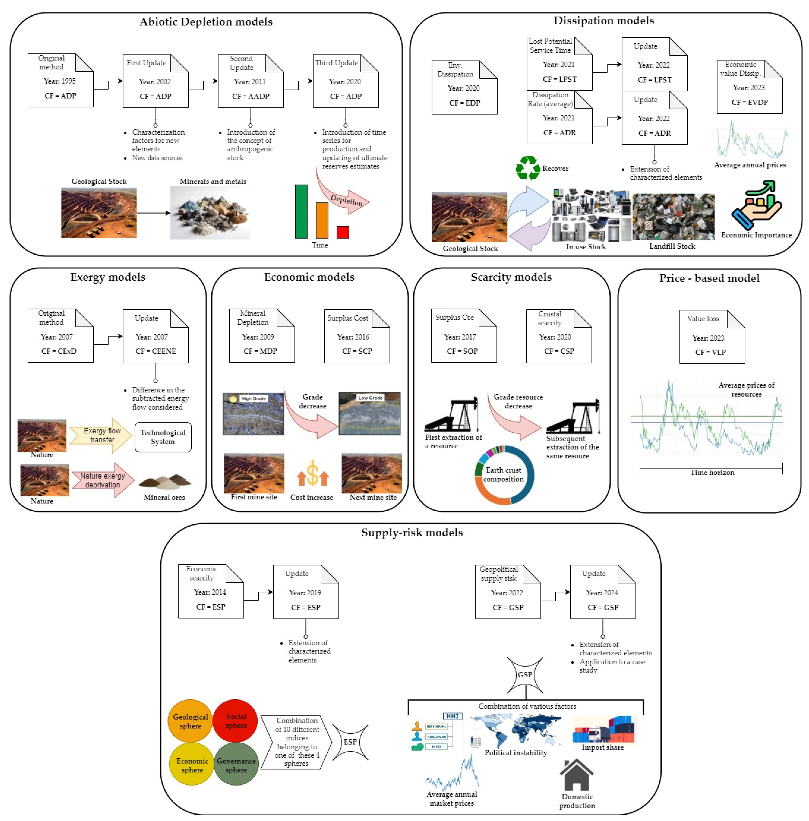
In the following sections, we will focus on the main characterization models for the use, depletion, scarcity, and criticality of mineral and metallic resources. Since the 1990s, researchers have increasingly focused on integrating the concept of mineral resources into LCA. The characterization models and their factors developed by different authors are described below, highlighting their mathematical formulation, main assumptions, data sources and limitations. Error! Reference source not found. list the CFs examined and related number of elements considered, while Error! Reference source not found. makes clear the boundaries of the analysis, distinguishing the methodologies into different families.
2.1. Abiotic Resource Depletion
The first major family of characterization models considered is abiotic resource depletion, which has been developed since the second half of the 1990s. The following paragraphs describe the original model and all subsequent updates and implementations.
2.1.1. Original Characterization Model
In a 1995 paper, Guinée and Heijungs [7] first approached the concept of resource depletion in LCA by developing equivalence factors per unit extracted. In the case of depletion, a distinction could be made between biotic and abiotic resources. Biotic factors are the living parts of an ecosystem (plant, trees, bacteria, etc.), while abiotic factors are non-living factors that affect an ecosystem (e.g. water, minerals and metals). In the original document, to quantify its depletion, they proposed a simple relationship calculated by summing the products of equivalence factors and the extraction amounts of different resources. Focusing on abiotic resources, the equivalence factors, called Abiotic Depletion Potentials (ADPs) are expressed by Eq. (1).
Where and respectively represent the production and the reserves of the resource “i” in a given period, while and production and reserve of a reference substance, which is antimony (Sb). In Eq. 1, the reserve term is squared to give greater weight, in terms of depletion, to those elements with a lower reserve for the same reserve-to-production ratio.
Figure 1.
Framework of characterization models considered in this review, grouped into families and developed by several authors.
Figure 1.
Framework of characterization models considered in this review, grouped into families and developed by several authors.
In the case of reserves, there are several terms with different definitions:
- “Reserve base”: part of an identified resource that meets certain minimum physical and chemical criteria related to current mining and production practices, including grade, quality, thickness and depth [2];
- “Economic reserve”: part of reserve base that can be extracted or produce economically at the time of determination [2];
- “Ultimate reserves”: reserves estimated by multiplying the concentrations of chemical elements in the Earth’s crust by its mass. It is also possible to add reserves in the oceans, and in the atmosphere to cover all primary means of extraction [7]; and
- “Ultimately extractable reserves”: technically extractable reserves [7].
Reference have referred to “Ultimate reserves”, calculated by considering the mass and the concentration of the Eart’s crust, the volume and concentrations of the oceans, and the mass and concentration of the atmosphere. The source of the element production data is a 1993 Report by the U.S. Department of the Interior [8], although specific data for some elements were missing. In case of completely missed data, rhenium (Re) was used as a reference. Yet, for the 6 Platinum Group Metals (PGMs), there was only one aggregate value, evenly distributed over the different elements. Finally, for compound mineral resources (e.g. TiO2, B2O3), the production data were allocated to the individual constituent elements according to their relative molecular weights. Given its relatively simple mathematical modeling, this method can be used to characterize the potential environmental impacts of various products in terms of resource depletion. However, many assumptions, including strong ones, have been made to obtain element-specific data. The updates to the methodology are discussed below, highlighting differences and improvements.
2.1.2. First Update of Characterization Model
In a study commissioned by the Dutch Ministry of Transport [9], an updated inventory was developed to implement the original abiotic resource depletion assessment method. Several changes were made to the original method:
- Calculation of characterization factors (CFs) using different estimates of extractable resources;
- Calculation of CFs for aggregates (such as lime, gypsum, etc.);
- Distinction between element depletion and fossil fuel depletion;
- Consideration of the multi-output process of refining metals after their extraction; and
- New data sources for reserve estimates.
Compared to the baseline method, ADP values were provided for individual elements in the case of ultimate reserves, reserve base and reserves, using 1999 as the base year. The estimation of ultimate reserves was done similarly to Guinée [10], while USGS data were used for reserve base and reserves. In the 1999 USGS Report [11], extraction and reserve values of various aggregates were given, and it was therefore possible to derive a CF for them. However, due to the absence of extraction rate data for certain elements, Guinée (1995) assumed they were extracted at the same rate as Re; these elements were not included in the update analysis. The ADPs obtained when considering three different resource types differ. Significant differences were found between reserve and reserve base, while similarities between reserves and reserve base. Given the uncertainty about which type of reserve is most appropriate for inclusion in LCA studies, the authors suggested considering multiple characterization models and conducting a sensitivity analysis to explore the impact on the results. The problem of moving from elemental CFs to mineral ones and vice versa has also been considered. Since ore may contain several elements, the problem arises of allocating the various energy and material inputs to the various outputs of the mining and refining processes. The allocation can be based on physical quantities (e.g. mass) or it can be economic. Another key aspect that emerged is the existence of reserves of elements in products within the Technosphere (especially in landfill) that could be recycled, avoiding the extraction of primary resources. This could be performed in the development of new models for assessing depletion in LCA.
This update of the original model has made some improvements and highlighted concepts for future implementation. Although the number of CFs is reduced compared to previous study – which might be seen as a limitation – the current approach employs more robust data without relying on strong assumptions.
2.1.3. Second Update of Incorporating the Anthropogenic Stock Concept
In the model that considers anthropogenic stock for the assessment of resource depletion [12], new CFs were introduced. The term anthropogenic stock refers to the amount of an element present in society, regardless of its chemical form [13]. First, resources were considered in the formulation of ADPs instead of ultimate reserves, defined by the USGS as: “concentrations of naturally occurring solid, liquid, or gaseous material in or on the Earth’s crust in such form and quantity that economic extraction of a commodity is currently or potentially feasible” [13].
In Eq. (2) and represent the extraction rate of the element “i” and of antimony, respectively. and the resource of the element “i” and antimony respectively.
Once the ADPs for the resource had been formulated, the anthropogenic stock was added to them, resulting in the following relationship of new CFs (see Eq. 3).
A technique often used to assess element stock is Materia Flow Analysis (MFA). However, at the time the Anthropogenic stock extended Abiotic Depletion Potential (AADP) factors were developed, anthropogenic stock data derived from MFA were only available for a very limited number of elements. To overcome this limitation, these stocks were estimated as the cumulative extraction rate from 1990 to 2008 based on USGS data. It was assumed that the amounts of elements extracted before 1900 were negligible. Within the Technosphere, different types of anthropogenic stock can be distinguished: in use, hibernating, deposited or dissipated. The dissipated part of the stock, defined as the fraction lost through chemical reactions or leaching [14], should be subtracted from the total anthropogenic stock. In this study, the dissipate flow is neglected based on the results for copper (Cu) from a previous work [14]. However, because elements other than copper have different properties that may render their dissipated quantities non-negligible, an element-specific evaluation of dissipation is advisable for future implementations of the model. Furthermore, elements with a higher anthropogenic stock contribute less to depletion than those with low stock values. To compare the values of ADPs and AADPs, a fictitious inventory containing 1 kg of each metal considered has been proposed. The introduction of the anthropogenic stock has improved the overall assessment of depletion, but a major limitation is the development of CFs for only a few elements (10).
In a subsequent paper [15], a partial revision of the AADP model was proposed, allowing the number of elements for which a CF was available to be increased. This extension was made possible by a new estimate of the ultimate extractable reserves and consideration of the depth at which mining takes place. It was assumed that 0,01% of the total amount in the Earth’s crust down to 3 km is available for metals and 0,001% for co-elements [16]. Having calculated the volume of the continental crust to a depth of 3 km and knowing the crustal abundance, it is possible to calculate the amount of each element [17]. Although new factors have been developed, further improvements are possible, including:
- Consideration of resource dissipation;
- Distinction between base metals and precious metals; and
- Integration of the concept of quality loss of recovered materials in the definition of anthropogenic resource stocks.
2.1.4. Integrating Time-Series Production Data and Refining Ultimate Reserves Estimates
In a 2020 study [18], researchers aimed to expand the scope of the resources considered in the characterization model based on ADPs, as well as updating the production data and estimating global elemental reserves. To update the production data of different elements, reference was made to the 1900-2015 time series of the USGS [19] and the 1970-2016 time series of the British Geological Survey (BGS) [20]. For most elements, the USGS was used; when USGS data were unavailable, those from BGS report were considered. In the case of cerium (Ce), hafnium (Hf), ruthenium (Ru), and scandium (Sc) the reference is an European document developed in collaboration with Deloitte [21]. Compared to previous studies, a step forward was taken by considering disaggregated data for Rare Earth Elements (REEs) production, based on assumptions proposed in a 2019 paper [22]. Here, 11 large REEs deposits, in different geographical settings were considered, covering more than 80% of the total of these resources. The final reserves were derived using the composition of the upper continental crust in terms of major elements, as reported in Rudnick and Gao [23]. This document, considered the standard on geological science, also indicates the different thickness of the layers that make up the Earth’s crust.
The innovative contribution proposed by van Oers et al. [18] concerns the consideration of a fluctuation in ADP values due to variations in the production of individual elements. Two alternatives have been proposed to take account of fluctuations in production: one based on a moving average, and other on cumulative production up to a given year. In the case of the moving average, instead of annual production of an element, a 5-year average production is used, expressed as Eq. (4):
Where is the number of years considered in the average. The choice of a period of 5 years is a compromise between reducing fluctuations and identifying a trend. Using a longer period would solve the problem of fluctuations, but no trend line would be identified. The proposed relationship for cumulative production up to a given year is shown as Eq. (5):
They also proposed a calculation of the ADPs of individual elements by considering the production of a single year (2015), the average production over 5 years (up to 2015) and a cumulative production of 46 years (1970 to 2015). Comparing the ADP values for 2015 to those of the 5-year moving average, the latter are always lower or at most equal (only in case of two elements: antimony and barium) with a maximum percentage reduction of 35,3% for mercury (Hg). A comparison of the ADPs for 2015 to those of the cumulative production shows a maximum reduction of 75,3%, in the case of gallium (Ga), and a maximum percentage increase of 84,6% for arsenic (As).
In this update, the set of elements with an associated CF has been extended to include strategic commodities such as REEs. However, to derive the different ADPs, certain assumptions have been made, regarding both the extraction and the ultimate reserves of the different elements. To further improve the accuracy and completeness of the data used to construct factors, the assumptions should be reduced as much as possible or at least tested for validity after a certain period.
2.2. Resource Dissipation
Resource dissipation in LCA was first proposed by Rolf Frischknecht at the 55th Discussion Forum On Life Cycle Assessment (Zurich, Switzerland) in 2014 [24]. A fundamental question raised by scientists concerns the appropriate abiotic resource flow to be considered in LCA. Firstly, it is possible to assess separately the resources extracted from the natural environment and those used in a dissipative manner. In order to make this explicit in the impact assessment phase of LCA, an example was considered where aluminum is used only once and a case where it is recycled [24]. ADPs have been applied to the dissipative use of resources, derived as the difference between the resource actually extracted and those recycled. An issue that has remained open is the distinction between borrowing and dissipative use, although an economic feasibility approach based on recovering resources from waste has been proposed. Borrowing refers to the possibility of future use of a resource once it has been extracted, through recovery and recycling operation, whereas dissipative use is definitive.
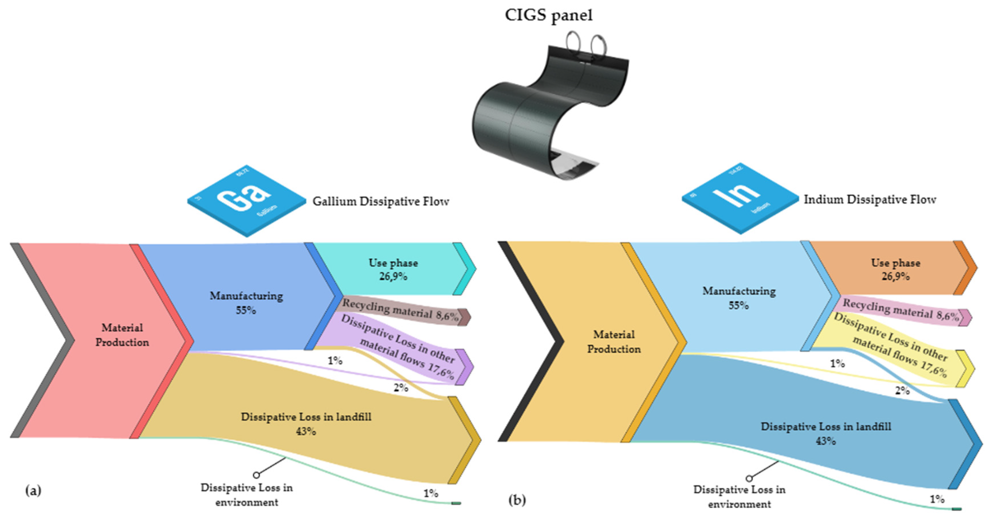
Ciacci et al. [25] evaluated the losses directly resulting from the design of various products for 56 metals and metalloids, distinguishing between: “dissipated in use”, “currently non-recyclable”, “potentially recyclable” and “unspecified”. A model based on economic allocation (global market share) to 4 material streams was proposed to measure the simultaneous loss of elements in the 4 identified groups. With this analysis, the dissipative concept was further refined and extended to numerous elements using the MFA technique. MFA approach to dissipative resource use is also applied in another 2016 study on products such as photovoltaic cells, catalysts and thermal barrier coating made in Germany [26]. The proposed methodology considers material inputs and outputs at all stages of the life cycle of the three products considered, based on industry data, literature data and expert considerations. For each product, key element flows have been considered, referring to a past year (2012) and to a future scenario (2030). Dissipative flows of indium (In) and gallium (Ga) were mapped for photovoltaic cells, germanium (Ge) for catalyst and yttrium (Y) for thermal barrier coating. The analysis of these fluxes allowed the identification of dissipation hotspots and recommendations for their reduction.
Figure 2.
Example of Gallium (a) and Indium (b) dissipative losses, in percent, for the 4 families identified by Zimmermann [26] in the 2012 scenario.
Figure 2.
Example of Gallium (a) and Indium (b) dissipative losses, in percent, for the 4 families identified by Zimmermann [26] in the 2012 scenario.
However, integrating the concept of dissipation into LCA databases is difficult by the need to quantify resource losses throughout the life cycle of products, as well as, the identification of contaminants in the waste stream. An initiative of the European Joint Research Centre (JRC) led to the development of a technical report in 2017 [27] with the aim of testing the feasibility of implementing dissipative resource use in LCA. To consider dissipation in LCA, it is necessary to act at two levels: at the level of Life Cycle Inventory (LCI) and of Life Cycle Impact Assessment (LCIA). In the case of the inventory, five alternatives were proposed:
- Identification of total, partial and null dissipation classes with possible partial dissipation subdivided into high, medium and low sub-classes;
- Consideration of resources in a binary “dissipated – non dissipated” (0-1) model;
- A “net approach” that avoids consideration of input and output flows for all unit processes;
- Determination of an average dissipated share and an average non-dissipated share; in practice, a simplification of the first alternative, where intermediate classes are not taken into account; and
- Identification of only dissipated flows with a net approach combined with a 0-1 approach.
Although each of these approaches has its own advantages and disadvantages, the fifth one was chosen in the feasibility analysis due to its practicality and the fact that it is essentially a synthesis of the first four. Once the approach was chosen, case studies were presented. One case starts with global copper stocks and flows in 2010 and arrives at the definition of dissipation rates that allow the construction of a specific inventory by life cycle phases (from extraction to end-of-life). The inventory obtained is compared with that of a “classical” depletion approach, which only considers mined copper and copper recycled at the end of its life. In both cases the ADP (ultimate reserves) factors are used to obtain results that show significant differences. The dissipative model allows a more precise identification by life cycle phase but does not show negative impacts compared to the depletion model. In conclusion, the report focuses exclusively on the inventory phase without considering the impact assessment phase. Although this paper does not focus on the impact assessment phase, it was considered consistent to present an initial overview of flow analysis to better clarify the concept of dissipation. We will now focus on the main characterization methods that have been developed to account for the dissipative effect.
2.2.1. Environmental Dissipation
The first approach to developing a comprehensive characterization method for assessing impacts in terms of dissipative flows has been carried out by a large group of researchers in 2020 [28]. The main objective of the work is to assess the future impact of current resource use by considering two time-horizons: short term (25 years) and very long term (500 years, from 2020 to 2520). The proposed system deals with naturally occurring stocks in nature and in the Technosphere and the material flows between them. Natural stocks are found in the earth, oceans and atmosphere, while those in the Technosphere are divided into stocks in use (in products) and stock in hibernation (in landfills, processing waste, or abandoned products). In the characterization model developed, the innovative element introduced concerns the variation in the accessibility caused by current use of resources. The proposed CF is constructed in a similar manner to the ADP, expressed with respect to a reference element (in this case copper), and is a function of two variables: the variation in the total accessible stock and the severity of making a resource inaccessible. The first variable is expressed by Eq. (6).
Where the term in the numerator represents the total global emission of a resource “i” at the time “t”, for the time horizon “T” considered. The term in the denominator is the total primary extraction added to the secondary supply of resource “i” in the year “t”.
The severity of the consequences resulting from the inaccessibility of a resource is presented by Eq. (7).
In this case, the denominator is the total accessible resource stock in the environment and Technosphere at the year “t+T” (i.e. the final year of the period considered).
Combining Eqs. (6) and (7) gives the CF for environmental dissipation, called Environmental Dissipation Potential (EDP):
In the very long-term case, it is possible to set equal to the current primary extraction (of 2020) and equal to the continental crust content of the resource “i”. Taking these assumptions into account, EDP is essentially analogous to ADP except that the first refers to total emission to the environment, while the latter to total extraction from the environment. If the same reference substance were considered, the two factors would be similar, but as they are different, there is a proportionality relationship (with a proportionality factor of 36,41). On the other hand, no CFs were proposed for short term (25 years) because of the large amount of data required (accessible stocks in nature and in the Technosphere, global flows of emitted, hibernated and occupied elements). But this could be an inspiration for future updates to the model.
Finally, in [28] a case study of two European copper companies is proposed, considering 1 kg of copper cathode as functional unit and system boundaries from cradle to gate. Both ADP and EDP factors were used to calculate the impacts, and the comparison showed a different relative contribution of the elements. Using the depletion method, almost all the impact is related to copper, while using the dissipation one, other elements, such as platinum, cadmium and silver contribute significantly. The two methods thus provide different perspectives: the depletion one focuses on the extraction of the resource that makes up the product under consideration, while the dissipation one considers emissions from all the processes that lead to the product (e.g. platinum contribute significantly to dissipation because it is used in explosive for mining).
2.2.2. Lost Potential Service Time and Average Dissipation Rate
A further development in the integration of dissipative flow of elements within LCIA methods was made in 2021 by Charpentier Poncelet et al. [29]. In their work, they proposed two methods based on Service Time (ST), defined as: “the service provided by a resource as a part of the stocks in use in the economy, after its extraction from nature and until its dissipation after one or more applications”. The total expected ST is the anthropogenic lifetime as reported by Helbig et al. [30].
The first method [29], called Lost Potential Service Time (LPST), considers the missed opportunity to use resources, once extracted, in relation to a target: the Optimum Service Time (OST). The choice of time horizon is crucial to reflect the possible interests of the various stakeholders and to be able to compare with other characterization methods. For this reason, three different time horizons were analyzed: 25, 100 and 500 years. In the case of short time horizon, a comparison with depletion potentials measured in terms of economic reserves may be of interest, while in the case of the long-time horizon, a comparison with depletion potentials in terms of ultimate reserves.
The second method [29], represented by the Average Dissipation Rate (ADR) indicator, refers to the overall annual dissipation rate of various metals, without considering any time horizon. For the calculation of the CFs in the two cases, data from 1997 to 2015 were screened, considering 29 end use sectors of the various metals, the yields of the main processes of each life cycle phase, and the dissipative uses. Charpentier Poncelet et al. [29] assumed the yield to be constant over time, and equal for all sectors. The mathematical formulations of the CFs in the two methods are given below, and starting with LPST, the factors are expressed with respect to a reference substance (iron) and refer to a precise time horizon (t.h.).
ST of a metal is calculating by summing its mass ratio in service, relative to time, over a given time horizon and relative to 1 kg of extraction. The OST is nothing other than the service time under theoretically optimal condition, i.e. with perfect yields.
In the case of ADR method, on the other hand, the factors are calculated as the inverse of the expected total service time of the metal “i” (see Helbig et al. [30]), with reference to an assumed infinite time horizon (which was 1000 years) and with reference to a substance (iron).
These two sets of CFs, calculated for 18 metals, provide a different interpretation of the total dissipation that occurs after an extraction. One considers the lost opportunity to use 1 kg of metal from the stocks in use in the economy, compared to a theoretical target of perfect yield (zero dissipation) and the other focuses on general extraction rates without considering a specific time horizon. The relative ranking of metals is essentially the same in both cases. The methods just described, apart from referring to a limited number of elements, are based on assumptions, some of which are very strong. For example, the yields of the different substances are not differentiated according to the production chains and applications. In addition, from the analysis of numerical factor values, it is not possible to distinguish the contributions of different dissipative processes along the life cycle of a product system. To overcome the problem of the limited number of resources considered, the same group of authors extended the number of metals characterized by dissipative flows, for both LPST and ADR factors, in a 2022 paper [31]. A further step in the work led to the assessment of the potential impact of resource dissipation in the socio-economic sphere, considering the fact that value and utility of a resource can be represented by its average price over a given time interval. Two new CFs have therefore been introduced at the damage level, which multiply for each resource its relative LPST and ADR by its average price over different time periods. A strength of the latter two factors is the possibility to obtain disaggregated data, with hypothesis, for 10 rare earths.
2.2.3. Dissipation Related to Economic Value
In the context of a framework for the development of LCIA methodologies, which is part of the broader SUPRIM project [32], it is possible to include a new method, developed in 2023, and related to the economic functions of abiotic resources [33]. This dissipative method, related to a short-term perspective (less than 10 years) focuses on two functions: recoverability function and value function. The first is expressed as a function of two variables and leads to the estimation of potentially dissipated resources, while the second determines the potential loss of value due to dissipation by assigning an economic value to the dissipated flows. The corresponding CFs are developed combining the two functions, which depend on the analyzed resource “a” and on the resource “x” in a given dissipative compartment.
The design of the recoverability function involved several steps and the analysis of several data sources. First, an overall average minimum grade was defined as the minimum concentration of resource derived from statistical analysis of data contained in a Standard and Poor’s database [34]. The minimum resource grade also varies depending on the dissipative compartment considered. The compartments include soil (earth’s crust), soil (upper continental crust), urban soil, air, water and landfill. The resulting recoverability function is dimensionless and varies between 0 (complete recovery) and 1 (complete dissipation).
When it comes to the value of a good, there is no consensus in economics on which quantitative indicator best represents it. For the structure of the value function, the price of a resource (understood as exchange value) and the economic importance, as defined by European Commission’s 2020 Criticality Study [35], were considered. Economic Importance (EI) depends on the share of a resource used (RS) in a given economic sector, the Value Added (VA) provided by the sector and the Substitution Index (SI), as shown below.
EI values vary between 0 (irrelevance of a resource for the EU economy) and 10 (irreplaceability for the EU). Once economic importance has been defined, it is possible to construct a value function that associates potential dissipation in mass terms with potential dissipation in monetary units.
Where “a” is the analyzed resource, “y” the year considered, the annual average price of a resource “a” (taken from USGS Report of 2021 [36]) and G a scaling factor. A criticality threshold is also set, based on expert judgment, corresponding to an EI of 2,8. The G factor is set precisely equal to 2,8 so that the potential dissipative loss of a resource with an EI of 2,8 is equal to the price. Sàntillan-Saldivar et al. [33] combined the values obtained for the two functions to develop a set of specific factors to environmental dissipation compartments and applied them to a case study on hydrometallurgical recycling of a lithium-ion battery. This work relates to a limited number of resources (15) and is based on various hypotheses, the most important of which relates to the recoverability of a resource. In fact, the study assumes that the main quantity for evaluating the potential recoverability of a resource is its concentration in a compartment and that recovery from a secondary source is like that from a primary source (mines). In addition, there is the way the value function is defined, a geographical limitation (reference to the EU), the need to update data for annual fluctuations in average resource prices and a possible revision of the indicators of economic importance in the case of new criticality studies.
2.3. Exergy Related Characterization Models
In thermodynamics, the term exergy first appears around the middle of the last century based on the concept of available energy. In the following years, the application potential of exergy was discovered in the context of assessing the environmental impact of resource exploitation using thermodynamics parameters. In 2007, researchers [37] proposed using exergy as an indicator of the energy quality of resources and to quantify the energy taken from the environment during product manufacturing. Exergy is thus inherent in resources and like energy, can be chemical, thermal, kinetic, potential, nuclear or radiative. For mineral resources and metals—which often consist of multiple chemical elements—they consider only chemical exergy. If the composition is known, chemical exergy can be calculated from the Gibbs free energy of formation and the exergy of the constituent elements. The CFs proposed for minerals and metals are none other than chemical exergy, expressed in energy per kg of substance “i”. For ores, since they often contain several extractable metals, an allocation factor is applied leading to the following formulation, as shown in Eq. (14).
Where is the chemical exergy, the mass fraction of the metal “i” in the ore, and the allocation factor for the element “i” (letters in brackets refer to the type of allocation performed: r stands for economic allocation based on revenue, while m stands for allocation based on mass). The main weakness of the methodology lies in the assumptions made to cover the lack of data on the composition of the resources and to solve the problem of the large variability of concentrations on a scale. An average composition was assumed for all ores, represented by the median exergy value of 0,63 MJ per kg of material. Thus, the difference between the CFs of metals contained in the ores is due to the metal concentration in the ores.
Meanwhile, another characterization model linked to the concept of exergy has been developed, called CEENE [38]. The developed idea combines the results of exergy analyses with product life cycle inventories from the Ecoinvent databases. This method is intended to be an implementation of the previous CExD method with some qualitative and quantitative variations. The main point of divergence between the two models lies in the subtracted energy flow considered. The CExD refers to the energy taken from the natural environment and transferred to a technological system, whereas CEENE assesses the energy flow deprived from nature. In the specific case of metals, different literature references are considered for the calculation of exergy, and quantitatively the first method considers the whole metal ore entering the Technosphere, while the second only takes into account ores containing metal fractions. CEENE consider 184 extraction flows from the natural environment (of which 79 related to minerals and metals) which can be divided into the following categories: fossil fuels, nuclear energy, renewable energies (wind, hydro and solar), metals, minerals and their aggregates, atmospheric resources, water resources and land use. The developed CF is defined as the exergy content per unit of specific flow (MJex/unit of flux). For some elements (e.g. aluminum), the total exergy involved in the extraction process is not fully accounted for because the materials are not completely pure and often consist of several chemical species. The different mineral species per element were obtained from industrial chemistry, extractive metallurgy handbooks, Ecoinvent database, and reports.
2.4. Economic Related Characterization Models
Extraction from a deposit always leads to the obtaining of several elements, given the simultaneous presence of different minerals. Mining operations, related to the obtaining of ore and metals, also have an economic aspect. To consider the potential impact of the depletion of a resource, previous studies [39] proposed a method focusing on the additional discounted cost that society incurs as a result of a mining operation. CFs were obtained for 20 elements, for a unit mass extracted, by combining various economic quantities, as can be seen in Eq. (15).
is the marginal cost increase in $/kg2, that is the ratio of the cost increase to the mass extracted that caused that price increase. on the other hand, represents the amount of resources produced in a certain period, while is the net present value, considering a specific time interval ΔT. Since a key quantity in the calculation of net present value is the discount rate, CFs have been proposed at four different discount rates: 2%, 3%, 4% and 5%.
In addition to the definition of the CFs at the damage or endpoint level (Eq. 15), they also proposed ones at midpoint level, named Mineral Depletion Potential (MDP) related to change in grade of a mineral, intended as a decrease in the concentration of a mineral caused by extraction [39]. As with most midpoint CFs, a reference substance was used (iron in this case). Due to the mathematical complexity of the model on underlying these midpoint factors, we do not present the formulas here and instead refer readers to the original document for detailed equations. This complexity, coupled with the extensive data required on global mineral deposits, explains why factors have been developed for a limited number of elements.
Another economic perspective on resource depletion considered co-production and the specific differences in costs between mines. In a 2016 study, Vieira et al. [40] reasoned about the average cost increase caused by future mining, since the first mines to be exploited are those with the lowest costs. To quantify the future economic scarcity of a resource associated with its extraction, the following factors were defined in Eq. (16).
Where is the determined operating cost derived from the cost-tonnage curve of metal “i” as a function of its extraction . the global maximum tonnage of metal “i” ever extracted and the current cumulative tonnage of metal “i” extracted. The cost-tonnage relationship can be approximated by a log-logistic distribution and refers to the period 2000 – 2012 or 2000 – 2013, depending on the metal. For this simplification authors followed their previous work [41] where the log-logistic distribution was applied to the grade-tonnage of copper.
The data needed to derive the characterization factors for 12 individual elements and one group of elements (Platinum Group Metals) are taken from a wide variety of sources, including: historical statistics of minerals in the U.S., reports from the Nuclear Energy Agency, reports from the U.S. Geological Survey and a UNEP document on long-term global metal stocks. Analysis of the CFs for the different metals showed a maximum variation of six orders of magnitude, with iron having the minimum value and rhodium the maximum value. The application of these factors, however, has several restrictions mainly related to the non-consideration of parameters such as the type of mines and minerals and the lack of attention to recent technological developments. Other weaknesses are inherent in the small number of characterized resources and the presence of a single aggregate value for Platinum Group Metals (PGM).
2.5. Scarcity Related Characterization Models
Often in the literature the terms scarcity and depletion are used indistinctly [42] even though they pertain to two different spheres: the first is more connected to the economic sphere, while the second to the geological one. In a 2010 paper, developed by the Hague Centre for Strategic Studies (a Netherlands study centre) [43], an attempt was made to clarify the concept of mineral scarcity by relating it not to the depletion of existing stocks but to the quantity extracted that becomes profitable in current market conditions. Scarcity therefore presupposes a dynamism of mineral reserves and its possible occurrence in the future depends not only on the quantity of these but on a series of related factors, including supply and demand, mining technology and the price of minerals. After this appropriate clarification, the main characterization methods proposed in the LCA field to consider the scarcity of resources are presented.
The first of these is related to the concept of the grade of a mineral, i.e. the concentration of desired material within it, and has been treated by Vieira et al. [44]. The developed CF considers the decrease in future grade after several extractions of a resource; therefore, to obtain the same amount of a material in the future, additional ore extraction will be necessary compared to the past. The expression of the factor, called Surplus Ore Potential (SOP), is completely analogous to that of the Surplus Cost Potential (SCP) factor illustrated above, except that the cost-tonnage relationship is replaced by the grade-tonnage relation, which is calculated by Eq. (17).
is the concentration of ore extracted for a certain amount of extracted resource . represents the maximum quantity to be extracted of a resource “i” and the currently known cumulative quantity (in tonnes) of the resource “i” extracted globally. As already done in the case of other CFs, it is possible to take a substance as a reference. The choice fell on copper, being the element for which the log-logistic distribution was originally applied to the grade-tonnage relationship.
With this methodology, 18 resources were characterized, and given the presence of several reserve definitions, two sets of factors were developed. The first referred to global reserves, as specified by the USGS, while the second referred to ultimate recoverable resources, defined by UNEP as 0,01% of the total amount of resources within the Earth's crust, considering a depth of 3 km. In both cases, the final analysis revealed differences between elements of 5 orders of magnitude (where manganese and iron have the lowest values while gold the highest). For the calculation of the mineral extracted for each resource, an economic allocation was made based on revenues, intended as the average price of resources for a period of 5 years. This time interval was chosen with the aim of reducing the influence of price variability as much as possible. Among the various points that can be improved there is certainly the limited coverage of resources and the consideration of the grade alone as a determining quantity for the exploitation of a mine. In addition to this, there are also intrinsic limitations related to the choice of the type of resource considered.
A further study developed based on the idea of scarcity is that of Arvidsson et al. [45]. In this case, however, the focus was on the concentrations within the Earth's crust of the various resources with the intention of creating a proxy for long-term global scarcity. The importance of the crustal content is related to the fact that it is stable over time and is associated with various measures of reserves and deposits. The crustal concentration, for these reasons, has been chosen as the only quantity for the mathematical relationship expressing the Crustal Scarcity Potential (CSP) factors, as shown in Eq. (19).
The choice of reference substance fell on silicon, the most abundant of those considered. A simple relationship such as Eq. (19) leads to several advantages, including the fact that it can include lots of materials with minimal effort in terms of data and information retrieval. It was possible to obtain disaggregated data for two important groups of metals: Rare Earth Elements (REEs) and Platinum Group Metals (PGMs). This is of fundamental importance for LCA practitioners who intend to approach the study of the life cycle of products containing these elements. Modeling simplicity can also be seen as a barrier since it means that not all aspects related to the use of a resource are considered. In addition, the long-term perspective may not consider possible short-term variations in the quantities of resources extracted, based on technological and economic needs.
2.6. Supply Risk-Based Characterization Models
The problem of insecurity linked to the supply of some strategic raw materials has always attracted the attention of companies and world governments. Since the early years of the twenty-first century, various scholars have tried to quantify this risk by proposing different indicators. In a 2013 review, Achzet and Helbig [46] considered 20 different indicators, both qualitative and quantitative, developed for the assessment of supply risk. A ranking was drawn up based on the frequency of use of these indicators, which saw the "country concentration" expressed by the Herfindahl-Hirschman Index (HHI) at its peak. This concentration index ranges between 0 and 1 and is a metric of the competition within the market. A value of zero indicates perfect competition, while a unit value indicates a monopoly. Other commonly used indicators include recycling potential, substitutability, dependence on imports and commodity prices.
In LCA, the first risk-based approach to resource supply was developed by Schneider et al. [47]. Compared to the conventional assessment of resource depletion, from a geological point of view, the integration of economic aspects allows a more complete analysis of industrial production with the opportunity to identify impediments in the supply chain. Unlike the CFs analyzed, the Economic Scarcity Potential (ESP) is presented as a dimensionless aggregate indicator, a combination of 10 different indices. These indices encompass geological, economic, social and governance spheres, and for each, a critical threshold is defined; exceeding this threshold implies an assumed supply risk. The supply risk is therefore expressed in Eq. (20) for each resource at the global average level.
Where subscript “i” indicates the various resources accounted for, and subscript “j” refers to the 10 indices relating to the various areas. The fact of including various areas in the evaluation is a strength of this methodology. In any case, it is also necessary to underline the limitations regarding the definition of critical values and the need for periodic updating of data, given the extreme changeability of global structures. In this analysis, equal importance is attributed to the various indices in the aggregation, while it could be of interest to an operator to assign different weights, considering the fact that the choice would imply additional uncertainty. Considering the above restrictions and emphasizing REEs due to their economic importance and the criticality related to possible supply disruptions, scholars [48] have analyzed and updated the various ESP factors for certain metals. The proposed methodological approach is very similar to that of Schneider et al. [47] except for the elements included in the analysis. In addition to including another set of elements, more up-to-date data sources were used where possible to better reflect the reality of the time. The result, in terms of ESP with equal weighting of the various indices, showed a predominance of REEs and PGMs, compared to elements such as gold, copper, iron and lithium. They also investigated the effect of changing the weighting of the indices. It was chosen to give greater weight to economic importance, so that it represents half of the final ESP score. In this different scenario, the ranking of the elements has varied compared to the base case of equal weighting. This highlights the relevance of choosing a weighing set in the decision-making process. In any case, the calculation to obtain a value of economic significance is very simplified and considers a limited number of variables. In addition, the production chain of the final elements is significantly streamlined, excluding some processing phases that it would be interesting to deepen.
Supply risk can also only be seen from a purely geopolitical point of view. In this context, characterization methods have been proposed. A first approach to integrating the geopolitical dimension in the LCA was introduced by Gemechu et al. [49]. The scope of the developed method is, in fact, identified in the LCSA, outside the present review but fundamental for the understanding of subsequent models. A calculation of geopolitical risk was proposed, differentiated by country, and based on import data and not on global production of materials. For the quantification of this risk, a factor expressed as a product between the HHI, and a risk mitigation factor was used, as indicated in Eq. (21).
HHI for the country “j” is evaluated by squaring each country’s market share of the global production of a specific commodity and then adding the resulting values. The mitigation factor, on the other hand, is expressed by summing the products of each country’s indicators of political instability (derived from the World Bank’s WGI) by , which is the import share of country “c” in the country’s market “j”. Eq. (21) was applied to 12 individual elements and 2 groups of elements (REEs and PGMs), considering the main global economies and the so-called emerging countries. The work of Gemechu et al. [49] was the starting point for the alignment of the geopolitical risk method with other typical midpoint indicators used in LCA, to which a mass flow can be associated.
In 2022, scholars [50] have operated this association, with the aim of harmonizing geopolitical risk assessment and LCA practices. Being a first attempt in this direction, a model was developed starting from a case study relating to four elements contained within a particular system produced: a lithium-ion battery. Eq. (21) has been appropriately modified by introducing both considerations relating to recycling as a risk mitigation factor and a new term, the average annual price in dollars of a certain raw material. As a result of these changes, the new CF, called Geopolitical Supply risk Potential (GSP), has been expressed as a function of resource "i" and a country "c" in a given year as in Eq. (22).
is the Herfindahl-Hirschman for raw material “i”, the geopolitical instability of country “j”, the import share of the resource “i” from country “j” to country “c”, the domestic production (with an estimate of recycled material included) of resource “i” in the country “c”. represents the total import of resource “i” into country “c” while the average annual market price of a given raw material “i”. The calculation of these factors was carried out on a very limited number of resources and in a geographical context limited to the European Union. Furthermore, as in the case of ESP, a periodic update of the data is essential given the changing geopolitical and economic scenarios worldwide. On the other hand, the structure of the geopolitical risk method makes it particularly versatile in providing valuable information related to specific places and time periods.
A further step in updating the geopolitical risk method was completed by researchers in a paper presented in July 2024 [51]. The main intention of the study was to demonstrate the potential of the method by expanding the number of resources characterized from a spatial and temporal point of view. To align the GSPs with other CFs implemented, copper was chosen as the reference to which the other elements were compared. In this way, GSPs are expressed in kg Cueq / kg of resource, as in the case of the SOP. Once the methodological choices were clarified, the results were presented, in terms of percentage contributions to the geopolitical risk of the individual elements contained within a photovoltaic laminate. The analysis of the results showed that some elements, although present in modest quantities within a product, can instead be dominant in terms of potential associated geopolitical risk. With this latest implementation of the method, a mature development of the concept of risk assessment of possible interruption of the supply chain of resources in the LCA field has been reached. However, research must not stop but must be oriented towards continuous improvement. Two possible directions of future research could be related to the evaluation of the uncertainty of the method and the investigation of the variations in terms of impact deriving from the choice of different data sources.
2.7. Price-Based Chracterization Model
In this section, a methodology for assessing future accessibility to mineral and metallic resources will be presented, developed by three authors [52] and not precisely attributable to any of the previous families. This method considers the value linked to the functions of minerals and metals within man-made products, assuming that the market price is a good approximation of this functional value. This assumption greatly simplifies the calculation of CFs, allowing them to be implemented for a wide range of resources. The mathematical expression behind the model is relatively simple and relates the average price of a certain resource, in a given time interval, with that of a reference substance (such as copper), as Eq. (23).
The prices of resources undergo, in the short term, fluctuations caused by a multitude of factors not necessarily related to their usefulness. To minimize these oscillations, they considered several time horizons of several decades, also conducting a sensitivity analysis to highlight variations in the results. In case copper is chosen as a reference and a 50-year perspective is considered, the elements with the highest factor are precious metals (such as gold and silver) and elements of the platinum group. A comparative analysis between Value Loss Potentials (VLPs) and ADPs (ultimate reserves) showed a weak correlation, given that the aspects related to resources in the two cases are different. For example, although germanium has a very low ADP, due to its relative abundance in the Earth's crust, it exhibits a high VLP because of its substantial price driven by strong demand in strategic applications such as photovoltaic cells, optical fibers and special glass. Although this methodology is based on limited assumptions and requires minimal data sources, it faces significant limitations concerning data completeness and uncertainty, as well as potential uninvestigated effects. Finally, given the recent implementation of this model and its limited application in case studies, potential critical issues may not yet have been identified.

Table 1.
Overview of the main characterization factors developed to account for the use of mineral resources in LCA and numbers of elements to which are associated.
Table 1.
Overview of the main characterization factors developed to account for the use of mineral resources in LCA and numbers of elements to which are associated.
| Characterization factor | Year | N° of elements1 | Authors |
|---|---|---|---|
| ADP (Abiotic Depletion Potential) | 1995 | 84 | Guinée [7] |
| ADP - first updating | 2002 | 41 + 14 aggregates | van Oers et al. [9] |
| AADP (Anthropogenic Abiotic Depletion Potential) | 2011 | 10 | Schneider et al. [12] |
| AADP - updating | 2015 | 35 | Schneider et al. [15] |
| ADP – second updating | 2020 | 76 | van Oers et al. [18] |
| EDP (Environmental Dissipation Potential) | 2020 | 76 | van Oers et al. [28] |
| LPST (Lost Potential Service Time) | 2021 | 18 | Charpentier Poncelet et al. [29] |
| ADR (Average Dissipation Rate) | 2021 | 18 | Charpentier Poncelet et al. [29] |
| LPST and ADR update | 2022 | 61 | Charpentier Poncelet et al. [31] |
| EVDP (Economic Value Dissipation Potential) | 2023 | 15 | Santillàn-Saldivar et al. [33] |
| CExD (Cumulative Exergy Demand) | 2007 | 107 | Bösch et al. [37] |
| CEENE (Cumulative Exergy Extraction from the Natural Environment) | 2007 | 79 | Dewulf et al. [38] |
| MDP (Mineral Depletion Potential) | 2009 | 20 | Goedkop et al. [39] |
| SCP (Surplus Cost Potential) | 2016 | 12 elements + 1 group of elements | Vieira et al. [40] |
| SOP (Surplus Ore Potential) | 2017 | 18 | Vieira et al. [44] |
| CSP (Crustal Scarcity Potential) | 2020 | 76 | Arvidsson et al. [45] |
| ESP (Economic Scarcity Potential) | 2014 | 17 | Schneider et al. [47] |
| ESP - updating | 2019 | 19 elements + 1 group of elements | Pell et al. [48] |
| GSP (Geopolitical Supply-risk Potential) | 2022 | 4 | Santillàn-Saldivar et al. [50] |
| GSP - updating | 2024 | 46 | Koyamparambath et al. [51] |
| VLP (Value Loss Potential) | 2023 | 66 | Ardente et al. [52] |
3. Focus on Rare Earth Elements
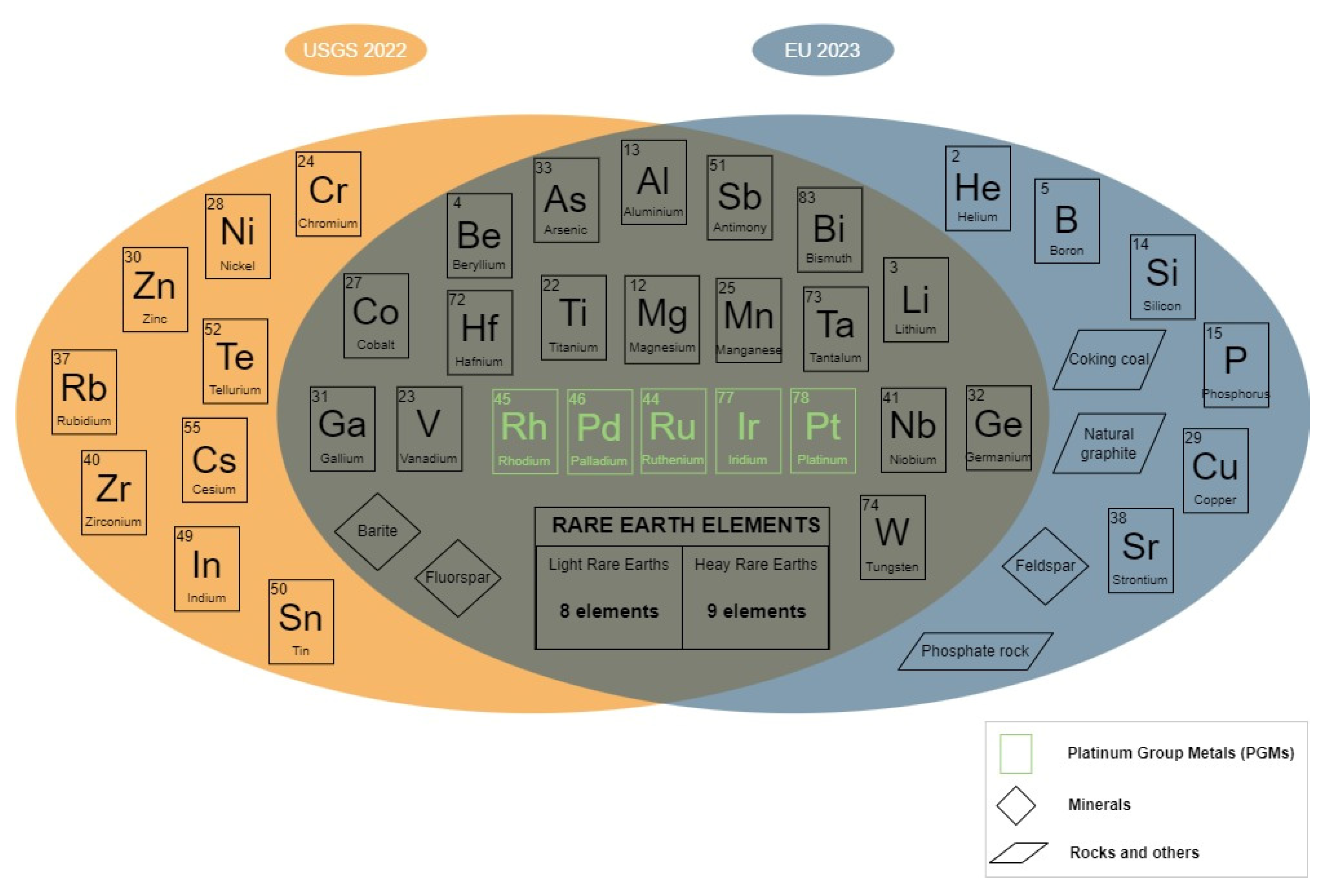
Rare Earth Elements (REEs) are considered critical raw materials by the European Union and various other national governments due to potential supply limitations arising from scarce availability and geopolitical instabilities, as well as their high economic importance stemming from their strategic role in high-tech applications. To clarify what these critical raw materials are and to monitor any changes, various efforts have been made at a global level, leading organizations like the EU and the U.S. Geological Survey to publish lists of these raw materials. The most recent series have been published in a 2023 European document [1] and a 2022 U.S. Department of the Interior report [53], and as shown in Error! Reference source not found. there are some elements in common.
Figure 3.
List of Critical Raw Materials by EU 2023 [1] and by USGS 2022 [53], showing common elements.
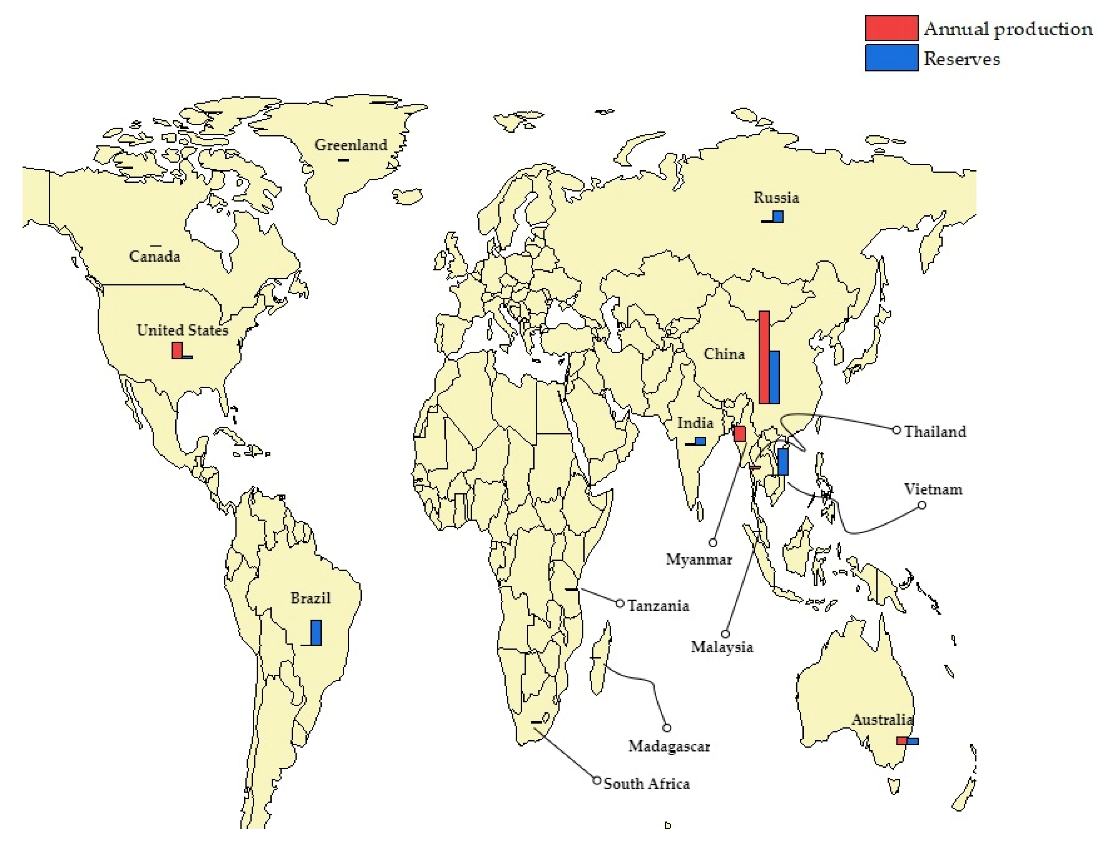
Among the common elements essential for many hi-tech applications, there are certainly REEs, used in technologies such as permanent magnets for electric motors, consumer electronics, batteries, LED screens and other high-performance materials. REEs include 17 chemical elements that are generally divided, based on atomic weight, into two groups: Light Rare Earth Elements (LREE) and Heavy Rare Earth Elements (HREE). The first group includes scandium (Sc), lanthanum (La,) cerium (Ce), praseodymium (Pr), neodymium (Nd), promethium (Pm), samarium (Sa) and europium (Eu) while the second group includes yttrium (Y), gadolinium (Gd), terbium (Tb), dysprosium (Dy), holmium (Ho), erbium (Er), thulium (Tm), ytterbium (Yb) and lutetium (Lu). These raw materials have a unique combination of properties that makes it difficult to replace them with other materials in many applications. This strategic importance is accompanied, however, by high costs associated with extraction and production, which over the years has led to a geographical confinement of processing in Asian countries, with China in the first position. As for global reserves, the largest holders are China, followed by Vietnam, Brazil, Russia, India and Australia. Error! Reference source not found. shows, the shares of annual production and reserves of rare earths in percentage terms, as reported in the 2024 USGS report [2]. As shown in Error! Reference source not found., countries, like Brazil, Russia and Vietnam potentially have a large amount of reserves but mainly due to the lack of suitable processing techniques the production is not so high. On the contrary, the United States ranks second in terms of global production despite having only one mine still operational.
Figure 4.
Annual production and reserves of REEs in the world, as reported in [2].
Figure 4.
Annual production and reserves of REEs in the world, as reported in [2].
To justify the focus on rare earths, the European Commission's 2023 report on critical raw materials [1] is considered. This document explains the methodology adopted for the criticality assessment, which essentially consists of identifying two thresholds for the parameters called Supply Risk (SR) and Economic Importance (EI). For SR, the threshold value is set at 1, while for EI at 2,8; and both must be exceeded to bring a raw material to be defined as critical. Both parameters, as reported in [54], are the result of the combination of various indices (including Herfindahl-Hirschman Index, Import Reliance, Substitution Index, Recycling Rate, Value Added of raw materials produced in the EU by economic sector, etc.). Error! Reference source not found. shows the values of SR and EI, present in [1], including copper and nickel due to their strategic importance. Although these metals do not exceed the SR threshold and therefore, strictly speaking, should not be classified as critical materials. Error! Reference source not found. demonstrates that the highest values are recorded in terms of SR (highlighted in red) for REEs. Conversely, regarding EI, only a subset of REEs—dysprosium, terbium, neodymium, praseodymium, and samarium—are relevant, while palladium, rhodium (both PGMs) and tungsten have the highest values. Finally, when combining the two factors discussed earlier, REEs emerge as the most critical, with dysprosium and neodymium occupying the top two positions in terms of criticality.
Table 2.
Supply Risk (SR) and Economic Importance (EI) of Critical Raw Materials [1].
Table 2.
Supply Risk (SR) and Economic Importance (EI) of Critical Raw Materials [1].
| Raw Material | Supply risk (SR) | Economic Importance (EI) | SR*EI |
|---|---|---|---|
| Aluminium | 1,20 | 5,80 | 6,96 |
| Antimony | 1,80 | 5,40 | 9,72 |
| Arsenic | 1,90 | 2,90 | 5,51 |
| Baryte | 1,30 | 3,50 | 4,55 |
| Beryllium | 1,80 | 5,40 | 9,72 |
| Bismuth | 1,90 | 5,70 | 10,83 |
| Boron | 3,60 | 3,90 | 14,04 |
| Cobalt | 2,80 | 6,80 | 19,04 |
| Coking coal | 1,00 | 3,10 | 3,10 |
| Feldspar | 1,50 | 3,20 | 4,80 |
| Fluorspar | 1,10 | 3,80 | 4,18 |
| Gallium | 3,90 | 3,70 | 14,43 |
| Germanium | 1,80 | 3,60 | 6,48 |
| Hafnium | 1,50 | 4,30 | 6,45 |
| Helium | 1,20 | 2,90 | 3,48 |
| Dysprosium | 5,60 | 7,80 | 43,68 |
| Erbium | 5,60 | 3,50 | 19,60 |
| Europium | 5,60 | 3,30 | 18,48 |
| Gadolinium | 3,30 | 3,30 | 10,89 |
| Holmium | 5,60 | 3,20 | 17,92 |
| Lutetium | 5,60 | 5,00 | 28,00 |
| Terbium | 4,90 | 6,40 | 31,36 |
| Thulium | 5,60 | 3,20 | 17,92 |
| Ytterbium | 5,60 | 3,20 | 17,92 |
| Yttrium | 3,50 | 2,90 | 10,15 |
| Lithium | 1,90 | 3,90 | 7,41 |
| Cerium | 4,00 | 4,90 | 19,60 |
| Lanthanum | 3,50 | 2,90 | 10,15 |
| Neodymium | 4,50 | 7,20 | 32,40 |
| Praseodymium | 3,20 | 7,00 | 22,40 |
| Samarium | 3,50 | 7,70 | 26,95 |
| Magnesium | 4,10 | 7,40 | 30,34 |
| Manganese | 1,20 | 6,90 | 8,28 |
| Natural graphite | 1,80 | 3,40 | 6,12 |
| Niobium | 4,40 | 6,50 | 28,60 |
| Iridium | 3,90 | 6,40 | 24,96 |
| Palladium | 1,50 | 8,10 | 12,15 |
| Platinum | 2,13 | 6,90 | 14,70 |
| Rhodium | 2,40 | 8,60 | 20,64 |
| Ruthenium | 3,80 | 5,50 | 20,90 |
| Phosphate rock | 1,00 | 6,40 | 6,40 |
| Copper | 0,10 | 4,00 | 0,40 |
| Phosphorus | 3,30 | 4,70 | 15,51 |
| Scandium | 2,40 | 3,70 | 8,88 |
| Silicon metal | 1,30 | 4,90 | 6,37 |
| Strontium | 2,60 | 6,50 | 16,90 |
| Tantalum | 1,30 | 4,80 | 6,24 |
| Titanium metal | 1,60 | 6,30 | 10,08 |
| Tungsten | 1,20 | 8,70 | 10,44 |
| Vanadium | 2,30 | 3,90 | 8,97 |
| Nickel | 0,50 | 5,70 | 2,85 |
Returning to LCA, as seen in the previous paragraphs, most of the resource characterization models either did not consider REEs or presented aggregated data. To overcome this issue, it is essential to map new mining projects and the flow of materials even at a regional level. In this sense, some studies have recently been conducted both globally and regionally. A first work was conducted by a group of researchers from Peking University [55] on an analysis of the flow of Nd material in China in 2016. In addition to primary production, imports and exports, consumption and loss of the resource during processing were also considered for a quantification of the change in stock. Another aim of the work was to separate aggregated data from rare earth mining production statistics into specific data relating to Nd alone. This was possible thanks to data on the composition of REEs contained in the various Chinese mineral deposits and the annual production of these sites.
In 2023, another group of researchers [56] conducted an analysis of mining projects reported by listed companies and governments, distinguishing between active mines and projects in an advanced stage of development. The distribution of resources is very diversified globally in terms of the quality and tonnage of the deposit, with sites defined as huge, such as Bayan Obo in China, Olympic Dam in Australia and Mountain Pass in the U.S., providing a contribution of more than half of the total resources. Advanced rare earth projects are distributed all over the world, but the continent with great potential in terms of deposits and therefore production is the African one, rich in carbonatites that are a possible source of REE deposits. If these processes were to be completed, there would be a diversification of the supply chain of REEs, which would no longer be almost exclusively the prerogative of China.
The two cases just presented could be taken as a starting point for the updating and implementation of the existing CFs related to individual REEs in LCA studies. A first attempt in this regard, in fact, has already been proposed in 2019 [22], exploring various data sources in terms of total reserves, extraction rates and average grade to obtain estimates for each element, considering 11 giant rare earth deposits. This served to achieve the goal of having single values in terms of ADPs based on less strong assumptions than those made, for example, by Guinèe [7] in the original depletion model.
Another key factor to be integrated into rare earth depletion impact assessment studies, in the LCA context, is certainly recycling, which can fill their growing demand and diversify the supply chain. In this way, by quantifying the potential recoverable resources, import-dependent countries could increase their autonomy with a lower risk of being exposed to market turbulence. Zhao et al. [57] evaluated the anthropogenic stock in use of REEs in 31 Chinese provinces, to quantify the end-of-life recycling potential of 9 products containing REEs. Old end-of-life technological products (such as wind turbines, electric vehicles, smartphones and e-bikes) constitute the so-called urban mines and the recovery of materials from them would allow the reduction of primary extraction with a series of environmental, economic and social benefits. The concept of urban mining refers to the possibility of recovering critical materials from the so-called stock in us, i.e. from old technological products, to reduce primary extraction and mitigate the environmental impacts deriving from the production of raw materials. A barrier to this potential is the absence, for the moment, of economically feasible technologies for the recycling of critical raw materials such as REEs.
4. Conclusions
This paper provides an overview of the main characterization models for mineral and metal resources in the LCA field, highlighting the methodological decisions and the main gaps to be filled. The various LCIA methods can be grouped into different families, depending on whether the underlying considerations relate to depletion, dissipation, scarcity, exergy, economic value, or supply risk. Although each LCIA methodologies adopts specific time horizons and emphasizes important aspects of resource use, there remains no international consensus on the most appropriate criterion for LCA studies. A persistent challenge across all LCIA models is the lack of complete, precise and up-to-date data on production, and on both natural and anthropogenic resource reserves.
An increasingly used technique to support the construction of CFs is Material Flow Analysis (MFA). By systematically evaluating material flows and inventories through mass balances, and accounting for spatial and temporal limitations, MFA could provide more granular and regionally specific data acquired both at regional and provincial level. This enhanced detail is crucial for accurately reflecting current conditions and guiding the sustainable management of mineral and metal resources. Such efforts align with the UN SDGs, underscoring the growing significance of both MFA and LCA in quantifying environmental impacts and identifying strategic intervention points. Although numerous characterization models currently exist for minerals and metals (abiotic resources), future research should explore the development of new indicators that integrate economic, social, and environmental dimensions. Such holistic approaches could facilitate decision-making by addressing sustainability more comprehensively. Additionally, updating existing models—both in terms of data and mathematical formulation—could improve their accuracy and relevance.
Furthermore, this review examines the issue of raw materials classified as critical by the EU and the U.S., specifying those considered critical in both contexts. Criticality is dynamic, influenced by market demand, supply constraints, and the availability of suitable substitutes. Among the critical raw materials, this review selects REEs as a focal point given their increasingly widespread use in many technologies, including permanent magnets used in hard-disk drives and in wind turbine generators, consumer electronics, batteries and high-performance materials for aerospace applications. Rapid growth in the production of electrical and electronic equipment in recent years has resulted in higher end-of-life concentrations of REEs in urban environments, prompting interest in “urban mining.” However, the economic feasibility of REE recovery from secondary sources remains limited, representing a significant barrier to unlocking their full circular economy potential.
In conclusion, strengthening data quality, exploring integrative indicators, and improving recovery technologies for critical resources like REEs are vital steps toward more sustainable and resilient resource management. Through continuous refinement and innovation, LCA complemented with MFA can more accurately capture resource dynamics and guide policy, research, and industry toward long-term global sustainability.
Author Contributions
Conceptualization, M.J. and A.M.; methodology, M.J.; validation, J.W., S.F. and A.M.; formal analysis, J..W.; data curation, M.J..; writing—original draft preparation, M.J.; writing—review and editing, J.W., S.F. and A.M.; supervision, J.W.; and A.M.; project administration, A.M.; funding acquisition, A.M. All authors have read and agreed to the published version of the manuscript.”.
Funding
This research is funded by the National Recovery and Resilience Plan (NRRP) and Ministero dell’Università e della Ricerca (MUR).
Institutional Review Board Statement
Not applicable.
Informed Consent Statement
Not applicable.
Data Availability Statement
Not applicable.
Acknowledgments
Conflicts of Interest
The authors declare no conflict of interest.
List of abbreviations
| 1. AADP | 2. Anthropogenic stock extended Abiotic Depletion Potential |
| 3. ADP | 4. Abiotic Depletion Potential |
| 5. ADR | 6. Average Dissipation Rate |
| 7. BGS | 8. British Geological Survey |
| 9. CEENE | 10. Cumulative Exergy Extraction from the Natural Environment |
| 11. CExD | 12. Cumulative Exergy Demand |
| 13. CF | 14. Characterization Factor |
| 15. CSP | 16. Crustal Scarcity Potential |
| 17. EDP | 18. Environmental Dissipation Potential |
| 19. EI | 20. Economic Importance |
| 21. ESG | 22. Environmental, Social and Governance |
| 23. ESP | 24. Economic Scarcity Potential |
| 25. EU | 26. European Union |
| 27. EVDP | 28. Economic Value Dissipation Potential |
| 29. GSP | 30. Geopolitical Supply risk Potential |
| 31. HHI | 32. Herfindahl-Hirschman Index |
| 33. HREEs | 34. Heavy Rare Earth Elements |
| 35. JRC | 36. Joint Research Centre |
| 37. LCI | 38. Life Cycle Inventory |
| 39. LCIA | 40. Life Cycle Impact Assessment |
| 41. LCSA | 42. Life Cycle Sustainability Assessment |
| 43. LPST | 44. Loss Potential Service Time |
| 45. LREEs | 46. Light Rare Earth Elements |
| 47. MCI | 48. Marginal Cost Increase |
| 49. MDP | 50. Mineral Depletion Potential |
| 51. MFA | 52. Material Flow Analysis |
| 53. NPV | 54. Net Present Value |
| 55. OST | 56. Optimum Service Time |
| 57. PGMs | 58. Platinum Group Metals |
| 59. REEs | 60. Rare Earth Elements |
| 61. SCP | 62. Surplus Cost Potential |
| 63. SDGs | 64. Sustainable Development Goals |
| 65. SI | 66. Substitution Index |
| 67. SOP | 68. Surplus Ore Potential |
| 69. SR | 70. Supply Risk |
| 71. ST | 72. Service Time |
| 73. USGS | 74. United States Geological Survey |
| 75. VA | 76. Value Added |
| 77. VLP | 78. Value Loss Potential |
References
- Study on the Critical Raw Materials for the EU, 2023. European Commission, Brussels.
- Mineral Commodity Summaries, 2024. U.S. Geological Survey, Washington.
- The 17 Goals | Sustainable Development. Available online: https://sdgs.un.org/goals (accessed on 04/12/2024).
- ISO – International Organization for Standardization, 2006. ISO 14040:2006 Environmental Management – Life Cycle Assessment – Principles and Framework. Geneva, Switzerland.
- ISO – International Organization for Standardization, 2006. ISO 14044:2006 Environmental Management – Life Cycle Assessment – Requirements and Guidelines. Geneva, Switzerland.
- Sonderegger, T.; Berger, M.; Alvarenga, R.; Bach, V.; Cimprich, A.; Dewulf J.; Frischknecht, R.; Guinée, J.; Helbig, C., Huppertz, T.; Jolliet, O.; Motoshita, M.; Northey S.; Rugani, B.; Schrijers, D.; Schulze, R.; Sonnemann, G.; Valero, A.; Weidema, B.P.; Young, S.B. Mineral resources in life cycle impact assessment – part I: a critical review of existing methods. Int J Life Cycle Assess 2020, 25(4), 784-797. [CrossRef]
- Guinée, J.B.; Heijungs, R. A proposal for the definition of resource equivalency factors for use in product life cycle assessment. Environ. Toxicol. Chem. 1995, 14(5), 917–925. [Google Scholar] [CrossRef]
- Mineral Commodity Summaries, 1993. U.S. Department of Interior – Bureau of Mines, Washington.
- van Oers, L.; de Koning, A.; Guinée, J.B.; Huppes, G. Abiotic resource depletion in LCA. Improving characterization factors for abiotic resource depletion as recommended in the new Dutch LCA Handbook; Road and Hydraulic Engineering Institute of the Dutch Ministry of Transport: Amsterdam, 2002; pp. 1-75.
- Guinée, J.B. Development of a methodology for the environmental life-cycle assessment of products: with a case study on margarines. PhD thesis, Leiden University, Leiden, March 2, 1995 https://hdl.handle.net/1887/8052.
- Mineral Commodity Summaries, 1999. U.S. Geological Survey, Washington.
- Schneider, L.; Berger, M.; Finkbeiner, M. The anthropogenic stock extended abiotic depletion potential (AADP) as a new parameterization to model the depletion of abiotic resources. Int J Life Cycle Assess 2011, 16(9), 929–936. [Google Scholar] [CrossRef]
- Mineral Commodity Summaries, 2010. U.S. Geological Survey, Washington.
- Kapur, A.; Graedel, T.E. Copper mines above and below the ground. Environ. Sci. Technol. 2006, 40(10), 3135–3141. [Google Scholar] [CrossRef] [PubMed]
- Schneider, L.; Berger, M.; Finkbeiner, M. Abiotic resource depletion in LCA – background and update of the anthropogenic stock extended abiotic depletion potential (AADP) model. Int J Life Cycle Assess 2015, 20(5), 709–721. [Google Scholar] [CrossRef]
- Skinner, B.J. A second iron age ahead? Am. J. Sci. 1976, 64(3), 158–169. [Google Scholar]
- Rankin, W.J. Minerals, Metals and Sustainability. Meeting Future Material Needs, 1st ed.; CSIRO: Calyton South VIC, Australia, 2011. [CrossRef]
- van Oers, L.; Guinée, J.B.; Heijungs, R. Abiotic resource depletion potentials (ADPs) for elements revisited – updating ultimate reserve estimates and introducing time series for production data. Int J Life Cycle Assess 2020, 25(2), 294–308. [Google Scholar] [CrossRef]
- Minerals information, 2018. U.S. Geological Survey, Washington https://minerals.usgs.gov/minerals/pubs/historical-statistics.
- World minerals statistics data, 2018. British Geological Survey, Keyworth (Nottinghamshire) https://www.bgs.ac.uk/mineralsuk/statistics/wms.cfc?method=searchWMS.
- Deloitte Sustainability; British Geological Survey; Bureau de Recherches Géologiques et Minières ; Netherlands Organisation for Applied Scientific Research. Study on the review of the list of Critical Raw Materials. Executive summary, 2017. European Commission, Brussels.
- Adibi, N.; LafhaJ, Z.; Payet, J. New resource assessment characterization factors for rare earth elements: applied in NdFeB permanent magnet case study. Int J Life Cycle Assess 2019, 24, 712–724. [Google Scholar] [CrossRef]
- Rudnick, R.; Gao, S. Composition of the continental crust. In Treatise on geochemistry, 2nd ed.; Holland, H., Turekjan, K., Eds.; Elsevier: Oxford, 2014; pp. 1–51. [Google Scholar]
- Vadenbo, C.; Rǿrbech, J.; Haupt, M.; Frischknecht, R. Abiotic resources: new impact assessment approaches in view of resource efficiency and resource criticality – 55th Discussion Forum on Lie Cycle Assessment, Zurich, Switzerland, April 11, 2014. Int J Life Cycle Assess 2014, 19, 1686–1692. [Google Scholar] [CrossRef]
- Ciacci, L.; Reck, B.K.; Nassar, N.T.; Graedel, T.E. Lost by design. Environ. Sci. Technol. 2015, 49, 9443–9451. [Google Scholar] [CrossRef] [PubMed]
- Zimmermann, T. Uncovering the Fate of Critical Metals. Tracking Dissipative Losses along the Product Life Cycle. J. Ind. Ecol. 2016, 21(5), 1198–1211. [Google Scholar] [CrossRef]
- Zampori, L.; Sala, S. Feasibility study to implement resource dissipation in LCA. Joint Research Centre (JRC) report, 2017. European Commission, Luxembourg. [CrossRef]
- van Oers, L.; Guinée, J.B.; Heijungs, R.; Schulze, R.; Alvarenga, R.A.F.; Dewulf, J.; Drielsma, J.; Sanjuan-Delmàs, D.; Kapmann, T.C.; Bark, G.; Uriarte, A.G.; Menger, P.; Lindblom, M.; Alcon, L.; Ramos, M.S.; Escobar Torres, J.M. Top-down characterization of resource use in LCA: from problem definition of resource use to operational characterization factors for dissipation of elements to the environment. Int J Life Cycle Assess 2020, 25, 2255–2273. [Google Scholar] [CrossRef]
- Charpentier Poncelet, A.; Helbig, C.; Loubet, P.; Beylot, A.; Muller, S.; Villeneuve, J.; Laratte, B.; Thorenz, A.; Tuma, A.; Sonnemann, G. Life cycle impact assessment methods for estimating the impacts of dissipative flows of metals. J. Ind. Ecol. 2021, 25, 1177–1193. [Google Scholar] [CrossRef]
- Helbig, C.; Thorenz, A.; Tuma, A. Quantitative assessment of dissipative losses of 18 metals. Resources, Conservation and Recycling 2020, 153. [CrossRef]
- Charpentier Poncelet, A.; Loubet, P.; Helbig, C.; Beylot, A.; Muller, S.; Villeneuve, J.; Laratte, B.; Thorenz, A.; Tuma, A.; Sonnemann, G. Midpoint and endpoint characterization factors for mineral resource dissipation: methods and application to 6000 datasets. Int J Life Cycle Assess 2022, 27, 1180–1198. [Google Scholar] [CrossRef]
- Schulze, R.; Guinée, J.; van Oers, L.; Alvarenga, R.; Dewulf, J.; Drielsma, J. Abiotic resource use in life cycle impact assessment – part II – linking perspectives and modelling concepts. Resources, Conservation and Recycling 2020, 155. [Google Scholar] [CrossRef]
- Santillàn-Saldivar, J.; Beylot, A.; Cor, E.; Monnier, E.; Muller, S. Economic value dissipation potential (EVDP): an improved method to estimate the potential economic value loss due to resource dissipation in life cycle assessment. Int J Life Cycle Assess 2023, 28, 1400–1418. [Google Scholar] [CrossRef]
- S&P Global Market Intelligence, 2022 S&P Capital IQ Online Database https://www.capitaliq.spglobal.com/.
- Study on the EU’s list of critical raw materials, 2020. European Commission, Brussels.
- Mineral Commodity Summaries, 2021. U.S. Geological Survey, Washington.
- Bösch, M.E.; Hellweg, S.; Huijbregts, M.; Frischknecht, R. Applying Cumulative Exergy Demand (CExD) Indicators to the ecoinvent Database. Int J Life Cycle Assess 2007, 12(3), 181–190. [Google Scholar] [CrossRef]
- Dewulf, J.; Bösch, M.E.; De Meester, B.; Van der Vorst, G.; Van Langenhove, H.; Hellweg, S.; Huijbregts, M. Cumulative exergy extraction from the natural environment (CEENE): a comprehensive life cycle impact assessment method for resource accounting. Environ. Sci. Technol. 2007, 41(24), 8477–8483. [Google Scholar] [CrossRef] [PubMed]
- Goedkop, M.; Heijungs, R.; Huijbregts, M.; De Schryver, A.; Struijs, J.; Van Zelm, R. A life Cycle Impact Assessment Method Which Comprises Harmonised Category Indicators at the Midpoint and the Endpoint level, first ed. Report; Ministerie van VROM: Den Haag, Netherlands, 2009 http://www.leidenuni.nl/cml/ssp/publications/recipecharacterisation.pdf.
- Vieira, M.; Ponsioen, T. , Goedkoop, M.; Huijbregts, M. Surplus Cost Potential as a Life Cycle Impact Indicator for Metal Extraction. Resources 2016, 5(2), 1–12. [Google Scholar] [CrossRef]
- Vieira, M.; Goedkoop, M.; Storm, P.; Huijbregts, M. Ore Grade Decrease As Life Cycle Impact Indicator for Metal Scarcity: The Case of Copper. Environ. Sci. Technol. 2012, 46(23), 12772-12778. [CrossRef]
- André, H.; Ljunggren, M. Towards comprehensive assessment of mineral resource availability? Complementary roles of life cycle, life cycle sustainability and criticality assessments. Resources, Conservation and Recycling 2021, 167, 1-12. [CrossRef]
- Kooroshy, J.; Meindersma, C.; Podkolinski, R.; Rademaker, M.; Sweijs, T.; Diederen, A.; Beerthuizen, M.; de Goede, S. Scarcity of Minerals. A strategic security issue, first ed. Report; The Hague Centre for Strategic Studies: Den Haag, Netherlands, 2010.
- Vieira, M.; Ponsioen, T. , Goedkoop, M.; Huijbregts, M. Surplus Ore Potential as a Scarcity Indicator for Resource Extraction. J.Ind.Ecol. 2017, 21(2), 381–390. [Google Scholar] [CrossRef]
- Arvidsson, R.; Ljunggren Söderman M.; Sandén, B.A.; Nordelöf, A.; André, H.; Tillman, A-M. A crustal scarcity indicator for long-term global elemental resource assessment in LCA. Int J Life Cycle Assess 2020, 25, 1805-1817.
- Achzet, B.; Helbig, C. How to evaluate raw material supply risks – an overview. Resour.Policy 2013, 38, 435–447. [Google Scholar] [CrossRef]
- Schneider, L.; Berger, M.; Schüler-Hainsch, E.; Knöfel, S.; Ruhland, K.; Mosig, J.; Bach, V.; Finkbeiner, M. The economic resource scarcity potential (ESP) for evaluating resource use based on life cycle assessment. Int J Life Cycle Assess 2014, 19, 601–610. [Google Scholar] [CrossRef]
- Pell, R.S.; Wall, F.; Yan, X.; Bailey, G. Applying and advancing the economic resource scarcity potential (ESP) method for rare earth elements. Resour.Policy 2019, 62, 472–481. [Google Scholar] [CrossRef]
- Gemechu, E.D.; Helbig, C.; Sonnemann, G.; Thorenz, A.; Tuma, A. Import-based Indicator for the Geopolitical Supply Risk of Raw Materials in Life Cycle Sustainability Assessment. J. Ind. Ecol. 2015, 20(1), 154–165. [Google Scholar] [CrossRef]
- Santillàn-Saldivar, J.; Gemechu, E.D.; Muller, S.; Villeneuve, J.; Young, S.B.; Sonnemann, G. An improved resource midpoint characterization method for supply risk of resources: integrated assessment of Li-ion batteries. Int J Life Cycle Assess 2022, 27, 457–468. [Google Scholar] [CrossRef]
- Koyamparambath, A.; Loubet, P.; Young, S.B.; Sonnemann, G. Spatially and temporally differentiated characterization factors for supply risk of abiotic resources in life cycle assessment. Resources, Conservation and Recycling 2024, 209, 1-9. [CrossRef]
- Ardente, F.; Beylot, A.; Zampori, L. A price-based life cycle assessment method to quantify the reduced accessibility to mineral resources value. Int J Life Cycle Assess 2023, 28, 95–109. [Google Scholar] [CrossRef]
- Final List of Critical Minerals 2022. U.S. Geological Survey, Washington.
- Methodology for establishing the EU list of critical raw materials – Guidelines, 2017. European Commission, Brussels.
- Geng, J.; Hao, H.; Sun, X.; Xun, D.; Liu, Z.; Zhao, F. Static material flow analysis of neodymium in China. J. Ind. Ecol. 2021, 25, 114–124. [Google Scholar] [CrossRef]
- Liu, S-L. ; Fan, H-R.; Liu, X.; Meng, J.; Butcher, A.R.; Yann, L.; Yang, K-F.; Li, X-C. Global rare earth elements projects. New developments and supply chains. Ore Geol. Rev. 2023, 157, 1–11. [Google Scholar] [CrossRef]
- Zhao, S.; Wang, P.; Wang, L.; Chen, W-Q. Quantifying provincial in-use stocks of rare earth to identify urban mining potentials in the Chinese mainland. J. Clean. Prod. 2024, 453, 1-13. [CrossRef]
Disclaimer/Publisher’s Note: The statements, opinions and data contained in all publications are solely those of the individual author(s) and contributor(s) and not of MDPI and/or the editor(s). MDPI and/or the editor(s) disclaim responsibility for any injury to people or property resulting from any ideas, methods, instructions or products referred to in the content. |
© 2024 by the authors. Licensee MDPI, Basel, Switzerland. This article is an open access article distributed under the terms and conditions of the Creative Commons Attribution (CC BY) license (http://creativecommons.org/licenses/by/4.0/).
Copyright: This open access article is published under a Creative Commons CC BY 4.0 license, which permit the free download, distribution, and reuse, provided that the author and preprint are cited in any reuse.


