Scour Near Offshore Monopiles, Jacket-Type and Caisson-Type Structures

1. Introduction

1.1. General

Many countries in coastal regions plan to utilize their offshore wind potential by developing offshore wind farms in water depths of 20 to 50 m. On a global level, Europe is still a market leader in offshore wind project construction (about 50%), followed by Asia (about 45%) and the US (5%). Various types of foundation structures of offshore wind turbines are used: monopiles, gravity-based structures and jacket/tripod structures.

The monopile is the most applied foundation type in shallow waters with a sandy soil covered with migrating sand waves. Gravity-based structures (GBS; caisson type foundation structures) are suitable for wind turbines in shallow water (up to 30 m) with sandy and rocky type soils. These types of structures generally have long skirts (often equal to the foundation height) under the foundation structures to prevent undermining. Jacket type structure can be used in deeper waters with depths up to 50 m. The scour near various types of structures is discussed in Section 1.2 to Section 1.4. Experimental and numerical methods are presented in Section 2. The new experimental results are analyzed in Section 3 and Section 4. Scour models and prediction results are given in Section 5. Summary and conclusions in Section 6.

1.2. Scour Around Monopiles

Many data sets of free scour around monopiles in laboratory and field conditions are available. Early work on this by Breusers et al. [1], Melville [2], Melville-Sutherland [3], Kothyari et al. [4], Melville [5], Lim [6], Melville and Coleman [7] goes back to current-related scour near circular bridge piers. They have found maximum scour depth values (d_s,max) in the range of 0.6 to 1.2 of the pile diameter (D_pile) expressed as: d_s,max=0.6 to 1.2 D_pile, depending on water depth, flow conditions, sediment size, and other factors. Cefas [8] measured maximum scour depth up to 5 m around the monopiles (D_pile=4.2 m; d_s,max=1.1 D_pile) of an offshore wind farm within coastal waters, on Scroby Sands, off Great Yarmouth (east coast of England). Similar values are reported by Rudolph et al. [9] for Q7 wind farm at 20 km offshore Holland coast and Raaijmakers et al. [10] for wind farm Luchterduinen, offshore the Holland coast.

1.3. Scour Around Gravity-Based Structures

Assessments on scour depth around circular gravity-based structures in laboratory conditions were done by [11,12,13,14,15,16]. Whitehouse [11] measured maximum scour depth values of 0.2 to 0.5 times the base foundation diameter (d_s,max/D_base=0.2-0.5) along circular caisson structures with long skirts (9.5 m) for high current velocities (u_o/u_cr=4 to 6) where u_o = the free-stream velocity upstream the structure and u_cr = the critical current velocity of motion of the sand seabed. Tavouktsoglu [15] measured values of d_s,max/D_base=0.3-0.65 for low current velocities (u_o/u_cr≅1.2). Sarmiento et al. [16] measured a maximum scour depth along a caisson structure of about d_s,max=0.125D_base after 5 hours in a movable bed scale model (d₅₀=0.15 mm) with water depth of 1 m and current velocity of 0.42 m/s (u_o/u_cr≅ 2). Whitehouse et al. [12] have summarized scour data for two field cases with gravity-based structures (GBS). The values of d_s,max/D_base are in the range of 0.05 to 0.12 for u_o,max/u_cr=4 to 5. Overall, the measured range is d_s,max/D_base=0.05 to 0.65, which is a rather large range indicating that the scour near GBS is sensitive to the precise structure dimensions, flow and sediment conditions.

1.4. Scour Around Jacket-Type Structures

Scour data near jacket-type structures are relatively scarce. Rudolph et al. [17] studied the scour near a jacket structure (open structure of multiple piles/legs) at block L9 of the Dutch North Sea sector, which was installed in summer 1997. The piles resting in the seabed (d₅₀ = 0.2 mm) have a diameter of D_pile in the range of 1.2 to 1.5 m. Typical depth-averaged peak flow velocities are 0.5 m/s during spring tide. Maximum far-field scour depths were measured in the range of 1.5 to 5.0 m and the near-field scour near the legs/piles (D_pile) was in the range of 2.0 to 3.5 m (about 1.5 to 2.5D_pile). The far-field scour hole (extent of bathymetrical changes relative to the undisturbed situation) had a radius of roughly 2.5 to 3 times the pile spacing. Bolle et al. [18] and Baelus et al. [19] analyzed scour depth around the jacket-structure at Thorton Bank offshore wind park in the southern North Sea. The maximum scour depth was in the range d_s,max=0.3 to 0.9D_pile. Welzel et al. [20] studied near-field and far-field scour around a jacket structure in a wave-current basin with water depth of 0.67 m (scale 1 to 30) and sand d₅₀ of 0.19 mm. The structure has four legs with pile diameter of 1.2 m. Current velocities varied between 0.1-0.4 m/s. The maximum far-field scour depth around the structure was about 1 m or d_s,max=0.8D_pile for sole current conditions. The maximum near-field scour depths around the least and the most exposed piles was d_s,max=1.3 to 1.75 D_pile for sole current conditions. Zhang et al. 2025 [21] used a 3D flow model to compute the near-bed flow and turbulence characteristics around a jacktet structure. An overview of most relevant and recent scour-related research of various types of offshore structures are given by Chambel et al. [22] and Sarmiento et al. [16].

2. Experimental and Numerical Methods

The prediction of the scour depth around these types of foundation structures in offshore conditions requires the application of numerical simulation models in combination with experiments in physical scale models. Both types of modelling tools are discussed in this paper.

New exploring experiments in a wide recirculating flume with steady flow conditions have been performed to determine the scour hole dimensions around a monopile, a jacket structure with 4 legs and a gravity structure (caisson type structure with monopile on top). The experiments have been performed in a small basin (10 by 2.5 m²) of the WaterProof laboratory. The hydrodynamic data (flow field) have been measured above a fixed model bottom (non-mobile). The water depth was about 0.35 m. The depth-averaged approach current velocity was about 0.26 m/s. The velocity profile at various locations around each structure was measured using a 3D NORTEK Vectrino instrument. In addition, streamlines were visualized by surface floats consisting of a small piece of wood with an aluminium body (cross) at a short line of 5 cm. All dimensions and conditions are given in Table 1.

After the flow experiments with a fixed bed, clear-water scour experiments were performed in the basin with a mobile sediment bed consisting of medium fine sand (d₅₀= 0.1 mm; d₉₀=0.18 mm; critical depth-averaged velocity for initiation of motion; u_cr=0.2 m/s). Each test was run until the maximum scour depth had reached equilibrium (after 5 to 20 hours). The scour depth data were derived from 3D-photographs after drying the model and from mechanical pointer gages.

The flow field and the scour details of these experiments are presented and used for validation of the scour models. Two types of scour prediction models have been used: 1) semi-empirical scour model SEDSCOUR and 2) the sophisticated SUSTIM2DV-model. Both models are explained in Section 5.

3. Experimental Results of Flow Around Monopile, Jacket Structure and Gravity-Based Structure

Figure 1, Figure 2 and Figure 3 show the measured velocity profiles at various locations for the monopile, GBS and jacket-type structure, respectively. The most characteristic features are:

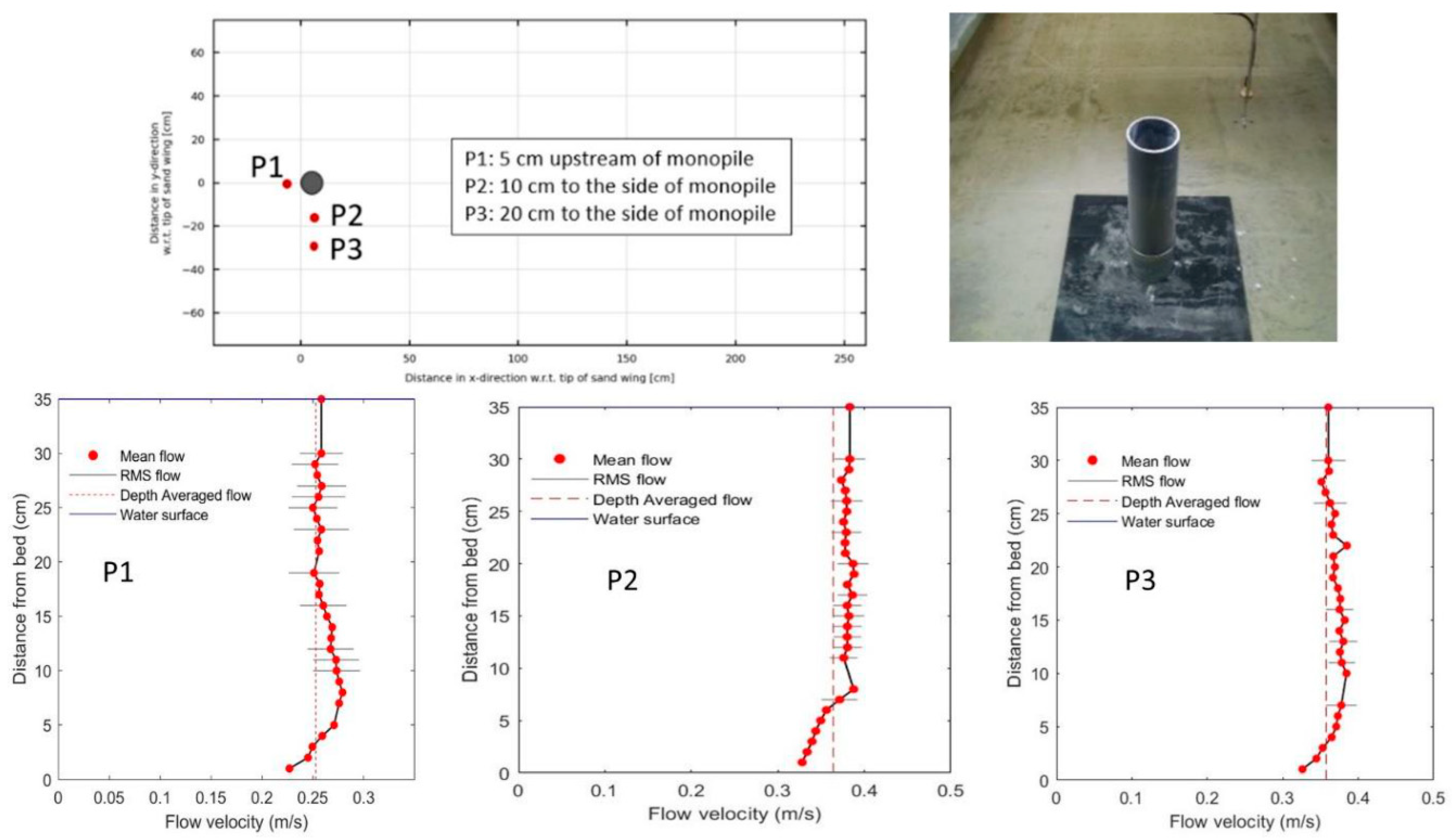
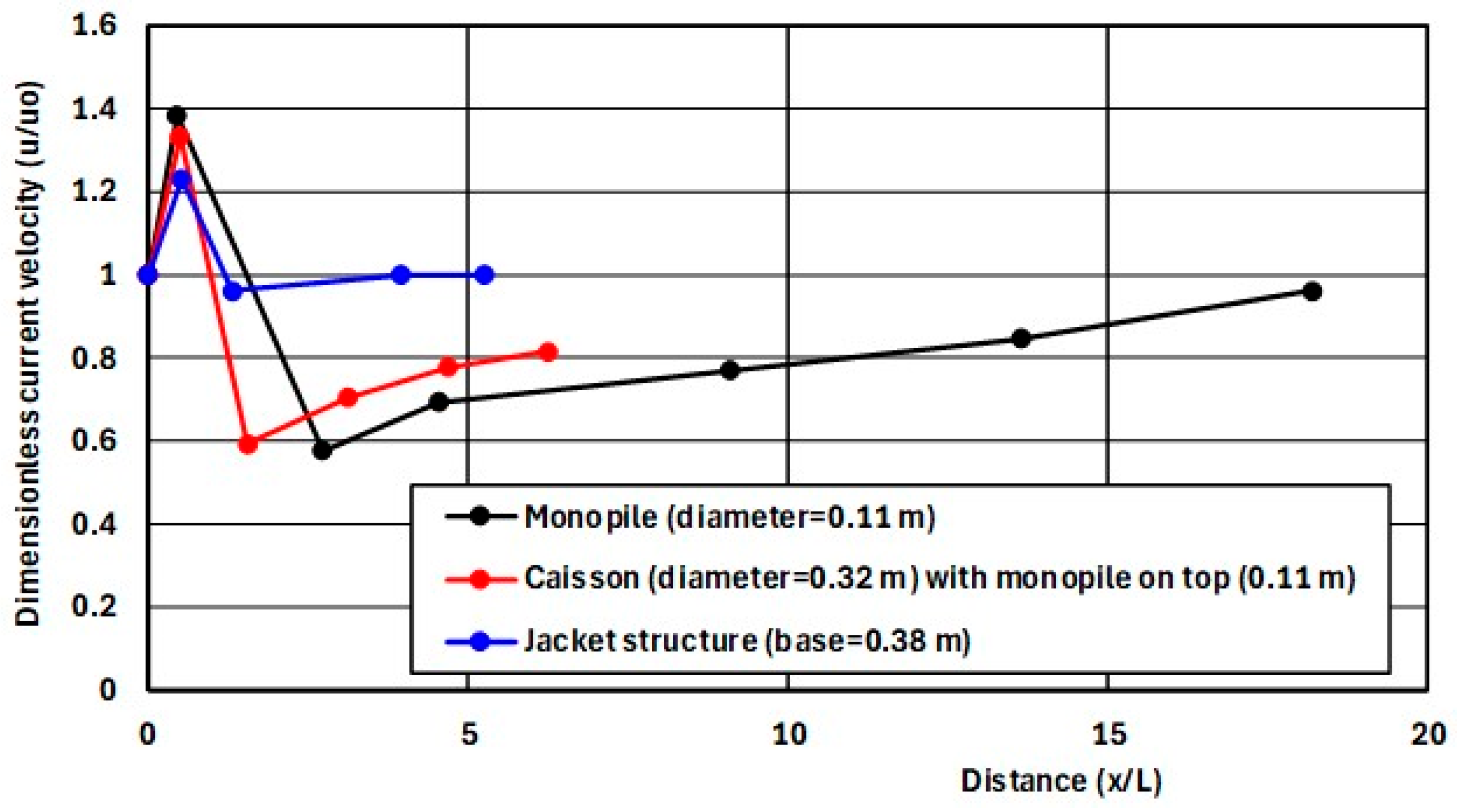
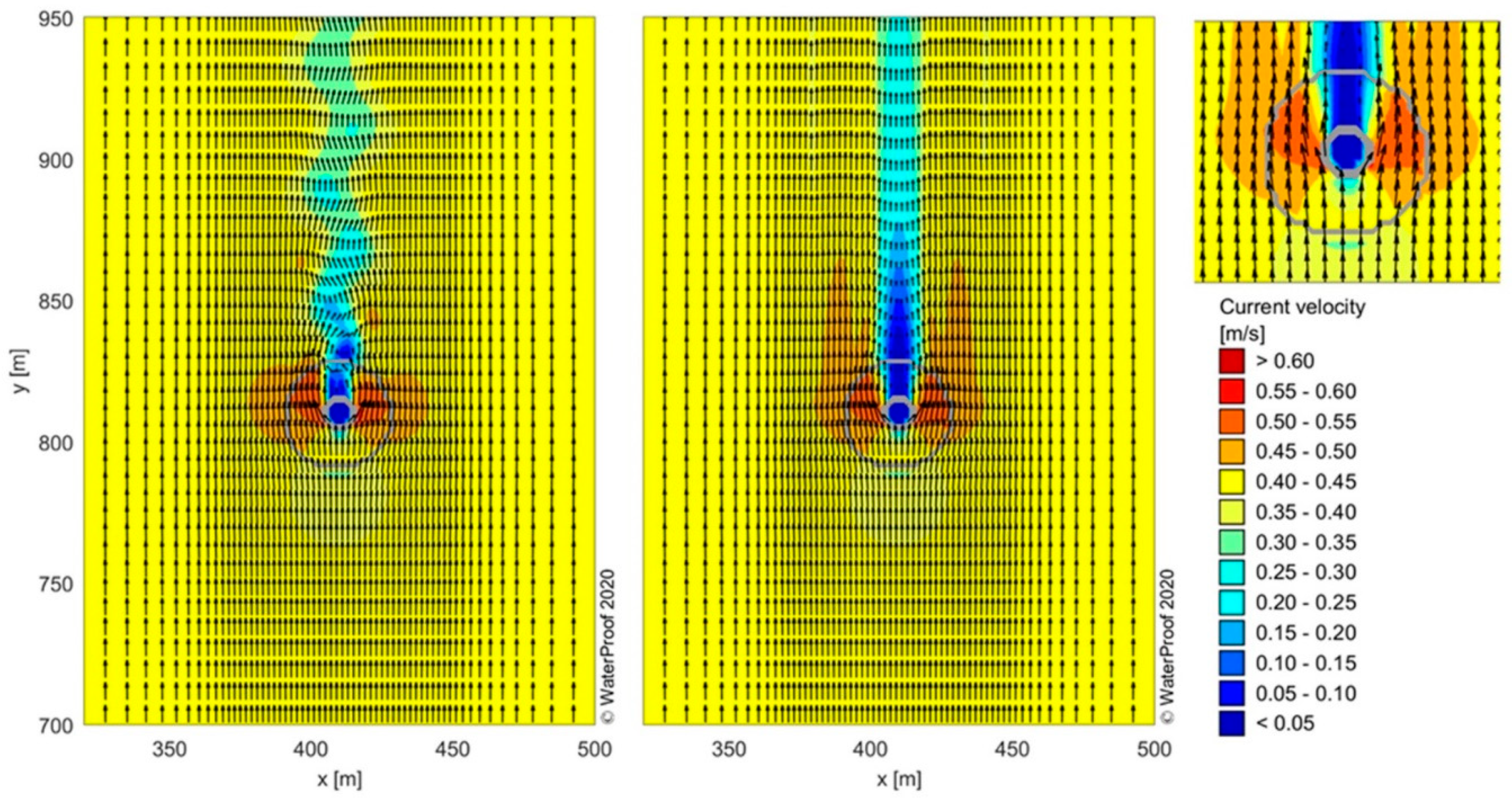
• monopile: significant increase of the approach depth-averaged flow velocity from 0.26 m/s at P1 to about 0.35 m/s at the flanks of the pile at P2 and P3; velocity profile is quite uniform over depth (accelerated flow);
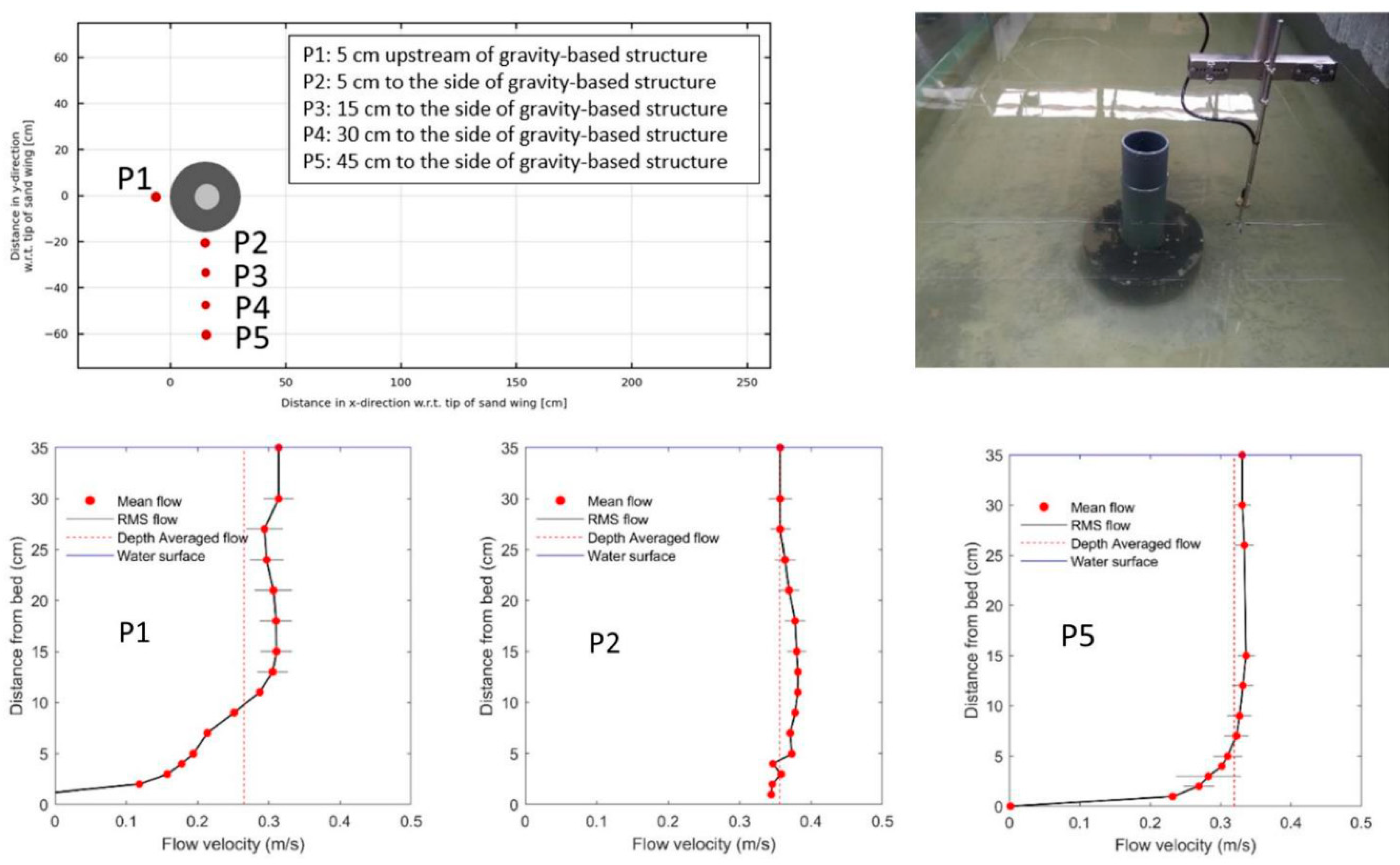
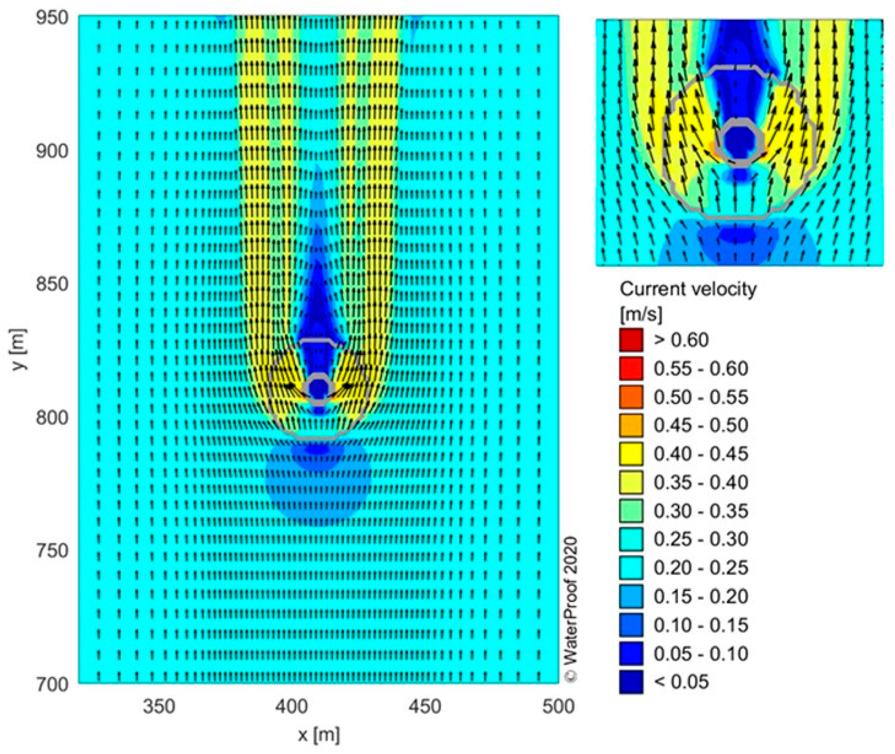
• caisson with monopile on top: significant increase of the approach depth-averaged flow velocity from 0.26 m/s at P1 to about 0.35 m/s on the flank of the caisson at P2; in turn, decreasing for larger lateral distances (0.32 m/s at P5); the velocity profile is rather uniform at P2, the velocity profile at P1 is slightly distorted, most likely due to effect of the downward-directed flow at the base of the structure.
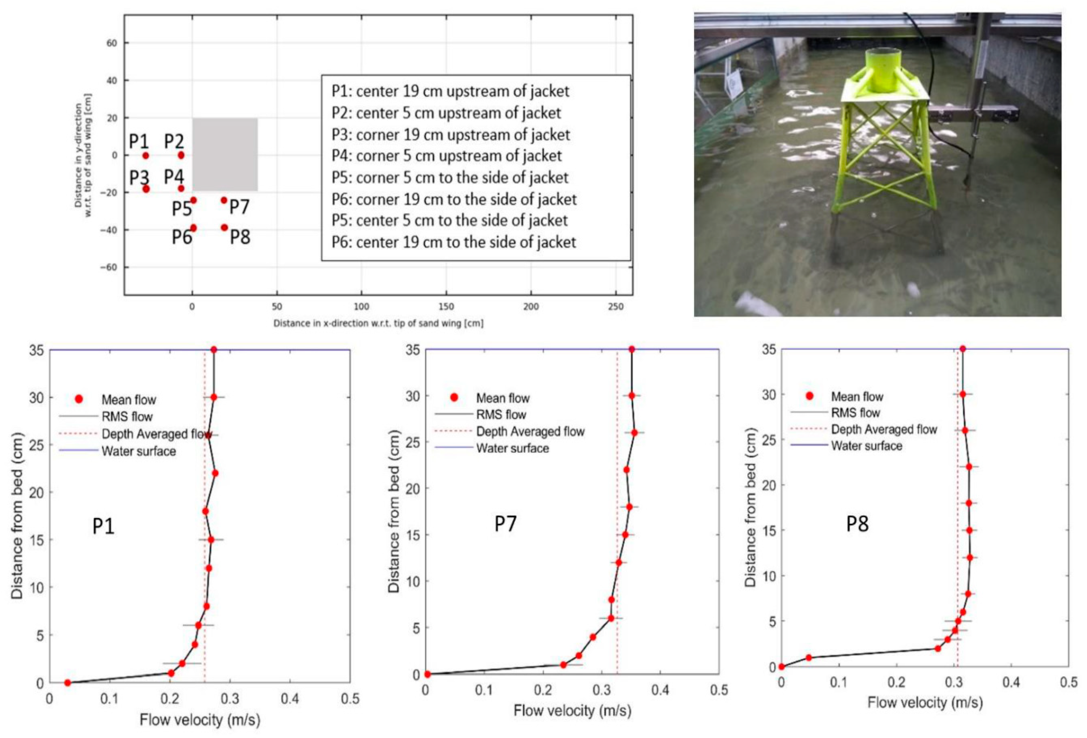
• jacket structure: increase of approach depth-averaged flow velocity from 0.26 m/s at P1 to about 0.30-0.33 m/s at P7 and P8, lateral of the structure; the vertical distribution of the flow velocities is rather similar.

Figure 1. Flow velocity field around monopile (D_pile=0.11 m).

Figure 1. Flow velocity field around monopile (D_pile=0.11 m).

Figure 2. Flow velocity field around caisson structure (D_caisson=0.32 m) with monopile on top (D_pile=0.11 m).

Figure 2. Flow velocity field around caisson structure (D_caisson=0.32 m) with monopile on top (D_pile=0.11 m).

Figure 3. Flow velocity field around jacket structure (D_leg=0.02 m; distance between legs=0.365 m).

Figure 3. Flow velocity field around jacket structure (D_leg=0.02 m; distance between legs=0.365 m).

Figure 4 shows flow lines based on near-surface floats. The flow lines are fairly straight for the open jacket structure and more curvy for the monopile and the caisson with pile on top.

Figure 5 shows the dimensionless depth-averaged velocity along the structure (monopile and caisson) and in the axis downstream of the jacket-structure. L is the structure length being L=0.11 m for the monopile, L=0.32 m (base diameter) for the caisson structure and L=0.38 m (base length) for the jacket structure. The upstream depth-averaged current velocity is 0.26-0.27 m/s for all structures. The current velocity strongly increases in the acceleration zone (0<x/L<0.5) with maximum value of about u/u_o≅1.4 for the monopile and decreases in the lee zone of the structures. The re-adjustment distance to free-stream velocities downstream of the monopile is about x/L≅20. A similar re-adjustment distance x/L≅15-20 seems present for the caisson-type structure. For the jacket-type structure this re-adjustment seems much shorter, because the flow interference is much less.

Figure 4. Flow lines for the 3 main experiments, obtained from tracking the position of near-surface floats.

Figure 4. Flow lines for the 3 main experiments, obtained from tracking the position of near-surface floats.

(flow from top to bottom).

Figure 5. Dimensionless depth-averaged velocity as function of dimensionless distance along structure.

Figure 5. Dimensionless depth-averaged velocity as function of dimensionless distance along structure.

4. Experimental Results of Scour near Monopile, JACKET structure and Gravity-Based Structure

4.1. Experimental Scour Results

The scour results for the three structures are presented in Table 2 and in Figure 6, Figure 7, Figure 8 and Figure 9. The most important scour characteristics are:

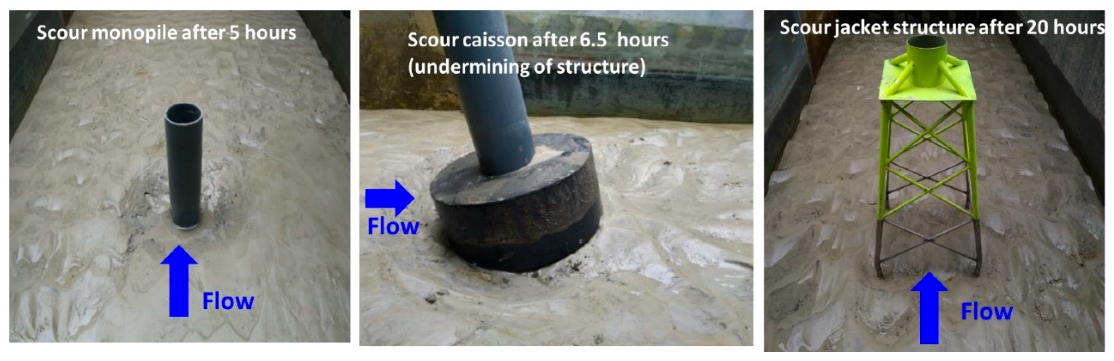
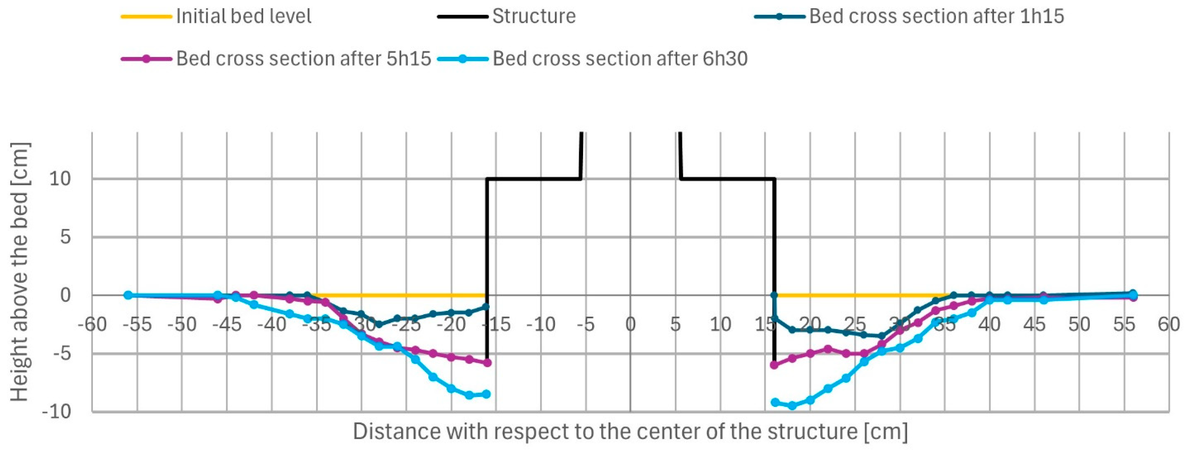
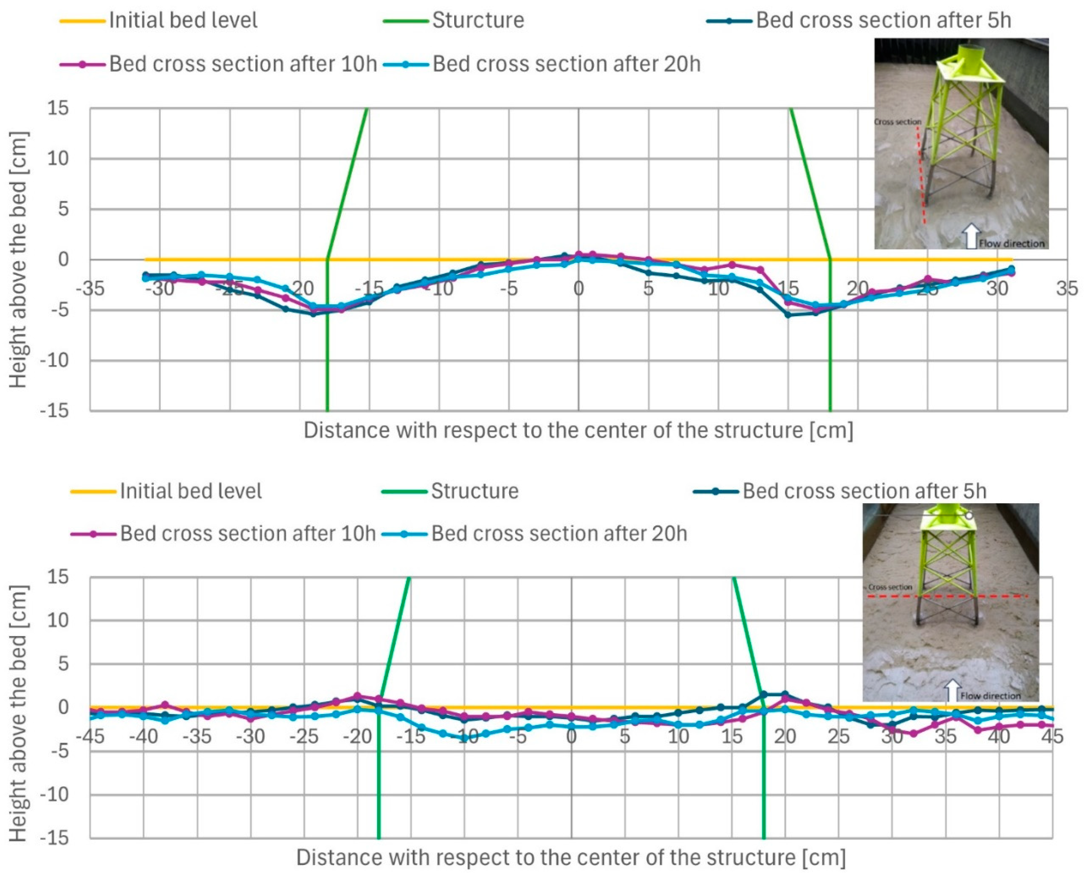
• monopile: maximum scour depth is d_s,max≅1.1D_pile after 5 hours with a maximum scour length L_s,max≅3D_pile at both sides;
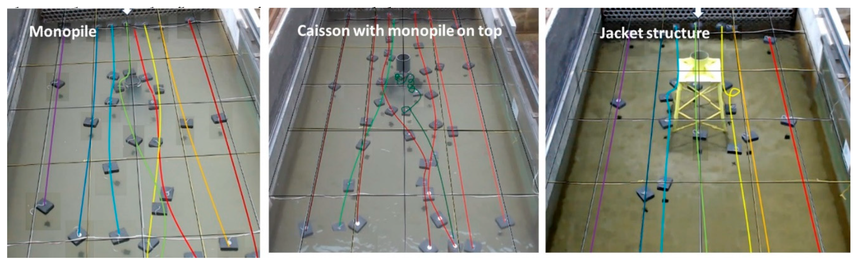
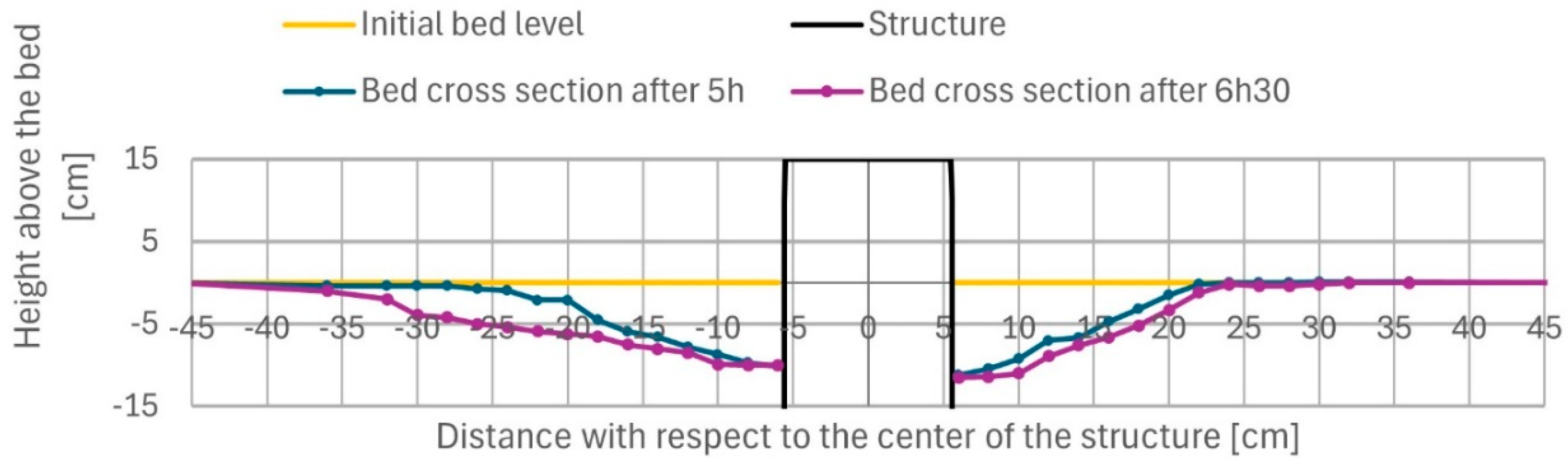
• caisson with monopile on top: maximum scour depth is d_s,max≅1 h_caisson (height of caisson) after 6.5 hours (at which the structure tipped over due to scour undermining, see Figure 6); maximum scour length L_s,max≅1 D_caisson at both sides;
• jacket structure: maximum scour depth near legs is d_s,max≅ 2.5D_leg after 20 hours; maximum scour length L_s,max≅10 D_leg at both sides; scour in center part under structure is lower (≅ 50% of scour depth near legs).

Table 2. Measured data from scour experiments; d₅₀=0.1 mm.

Parameter	Monopile	Caisson with monopile (GBS)	Jacket structure
Maximum scour depth	0.12 m (≅1.1Dpile)	0.10 m (≅1.0 hcaisson) (0.3 Dcaisson)	0.05 m near legs (≅ 2.5 Dleg) 0.03 m (≅ 1.5 Dleg) in middle structure
Maximum scour length	0.35 m (≅3 Dpile) on both sides of pile	0.3 m (1Dcaisson) on both sides	0.20 m (≅10Dleg) on both sides of leg

Table 2. Measured data from scour experiments; d₅₀=0.1 mm.

Parameter	Monopile	Caisson with monopile (GBS)	Jacket structure
Maximum scour depth	0.12 m (≅1.1Dpile)	0.10 m (≅1.0 hcaisson) (0.3 Dcaisson)	0.05 m near legs (≅ 2.5 Dleg) 0.03 m (≅ 1.5 Dleg) in middle structure
Maximum scour length	0.35 m (≅3 Dpile) on both sides of pile	0.3 m (1Dcaisson) on both sides	0.20 m (≅10Dleg) on both sides of leg

Figure 6. Scour near pile foundation structures.

Figure 6. Scour near pile foundation structures.

Figure 7. Scour near monopile.

Figure 7. Scour near monopile.

Figure 8. Scour near caisson with monopile.

Figure 8. Scour near caisson with monopile.

Figure 9. Scour near legs of jacket structure (2 cross-sections, see insets).

Figure 9. Scour near legs of jacket structure (2 cross-sections, see insets).

4.2. Discussion

Monopile structure: The maximum scour depth of the present tests with a monopile (d_s,max=1.1 D_pile) is of the correct order of magnitude compared to scour data from the literature (d_s,max=0.6 to 1.2 D_pile), thereby confirming the validity of the experimental setup.

Caisson structure with monopile (GBS): The maximum scour depth d_s,max=0.3 D_base for u_o/u_cr=1.3 is in the middle of the literature data range (d_s,max=0.05-0.65 D_base). Whitehouse [11] measured much larger scour depths of 0.2 to 0.5 times the base foundation diameter (d_s,max/D_base=0.2-0.5) for high current velocities (u_o/u_cr=4 to 6). Tavouktsoglu [15] also measured much higher scour values of d_s,max/D_base=0.3-0.65 for low current velocities (u_o/u_cr≅1.2). Sarmiento et al. [16] measured a maximum scour depth along a caisson structure of about d_s,max=0.125D_base after 5 hours in a movable bed (d₅₀=0.15 mm) scale model with water depth of 1 m and current velocity of 0.42 m/s (u_o/u_cr≅ 2).

Jacket structure: The absolute scour depth is much less (factor 2) than that around the other two types of structures see Table 2. The maximum scour depth near the leg of a jacket-structure is d_s,max=2.5D_leg while that near a monopile is about d_s,max=1.1D_pile, This means that the extra effect of the overall jacket structure on the scour near the legs is of the same order of magnitude. The scour depth d_s,max=2.5D_leg value measured during the present test (d₅₀=0.1 mm) is higher than the scour depth d_s,max=1.3 to 1.75 D_pile measured in the tests (d₅₀=0.19 mm) of Welzel et al. (2019) [20], which may be related to the somewhat coarser sand used by Wenzel et al.

5. Scour Modelling and Results

5.1. General

Two scour models are presented: semi-analytical 1D scour model (SEDSCOUR) for monopiles and jacket structure and numerical 2DV-model (SUSTIM2DV; [23,24]) for caisson type structures.

5.2. Scour near Monopile and Jacket Structure; Description of SEDSCOUR-Model

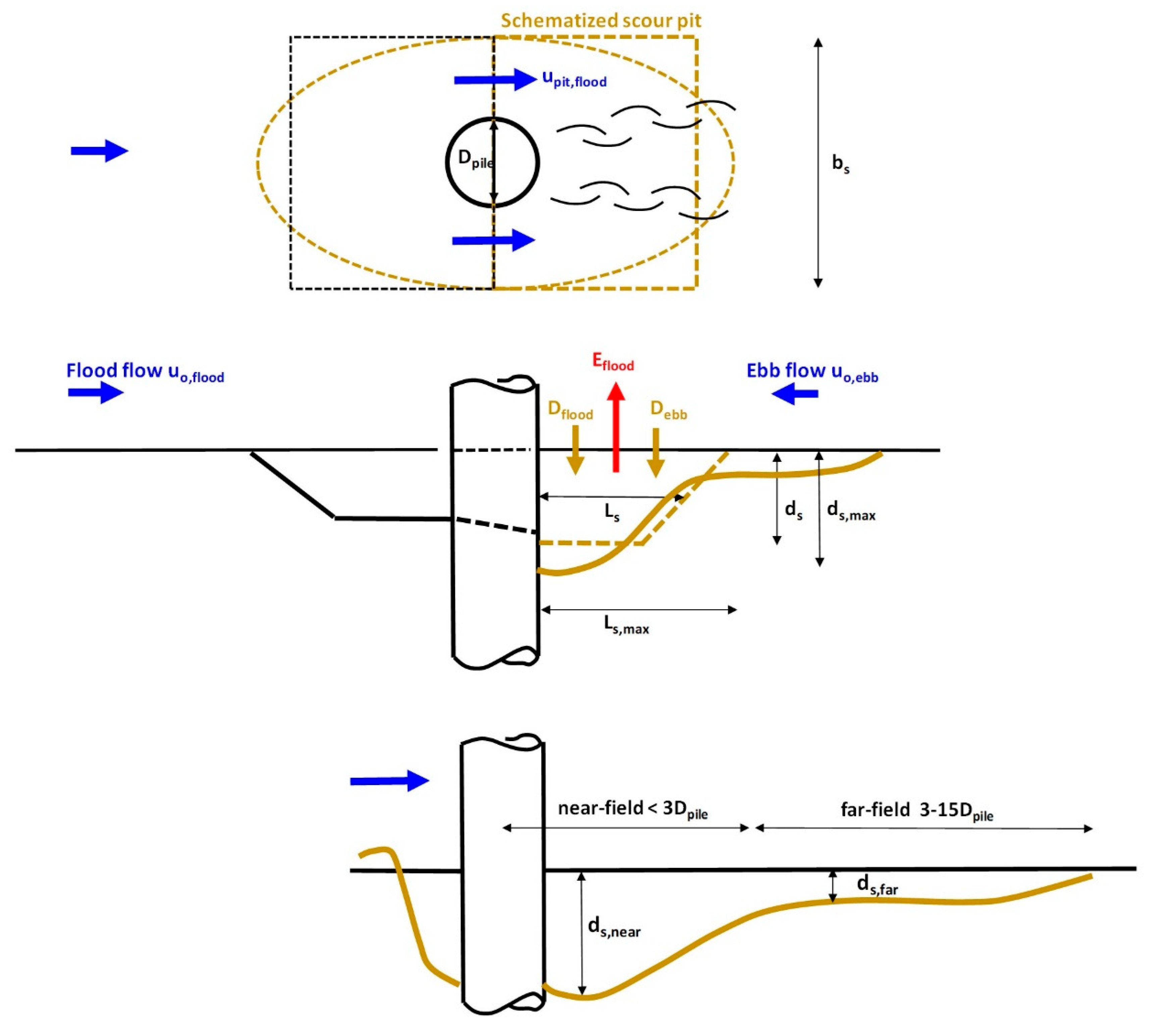
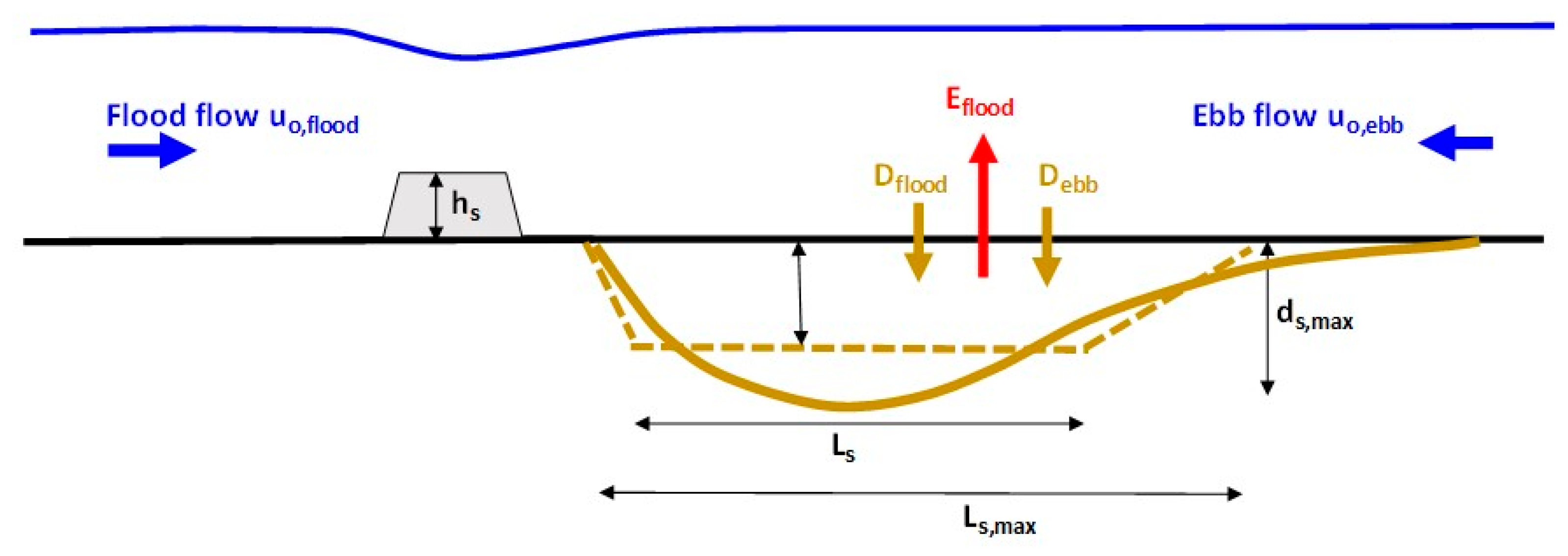
5.2.1. General Schematization

The free scour hole/pit generated around a pile-type structure (without scour protection) is schematized into two separated scour pits on the upstream and downstream sides of the pile, as shown in Figure 10. The deepest scour pit is generated in the lee of the pile downstream of the highest peak tidal current velocity (assuming a slight velocity asymmetry; u_flood>u_ebb). Both scour holes are similar in shape. Herein, it assumed that the flood current is dominant with the highest peak current velocity. Only the deepest scour hole (with scour depth d_s and length L_s) is considered (on the right in Figure 10). This scour pit consists of a deep scour pit near the pile and a shallow scour pit further away from the pile.

The tidal current is assumed to be perpendicular (normal) to the structure. Two tidal periods are considered: flood period of about 6 hours with one flood-averaged and depth-averaged velocity u_flood and similarly an ebb period of about 6 hours with one ebb-averaged and depth-averaged velocity u_ebb. Thus, each tidal phase (flood/ebb) is represented by one representative velocity. The variation of the flow velocity over the tidal cycle is not represented. The neap-spring variation of the velocities is represented by a sinusoidal variation based on input values. The scour pit erosion developing downstream of the pile over a tidal cycle of 12 hours is the net result of the following tide-averaged sand transport processes:

• flood: erosion of sand (E_flood) from the bed in the lee of the pile due to flow accelerations and increased turbulence levels; and deposition of sand (D_flood) from the incoming flood flow;
• ebb: deposition of sand (D_ebb) from the incoming ebb flow (after reversal of the tidal current).

The SEDSCOUR-model can also be used to compute the free scour downstream of a structure (obstacle) on the seabed such as a rock protection on a pipeline or a weir/sill in a river bed, see Figure 11. The trapping of sand from the incoming sediment load (if present) is taken into account.

The scour process is assumed to be a two-dimensional process. Therefore, the scour width normal to the tidal current is set to b_s=1 m (unit width). The mean scour length in the direction of the tidal current is assumed to be L_s=α_L h_s with h_s= upstream structure or obstacle height; α_L =input value.

5.2.2. General Model Equations

The deep part of near-field scour pit is represented in the SEDSCOUR-model as a rectangular box with dimensions: d_s=mean scour depth, b_s=mean scour width and L_s=mean scour length. The maximum scour depth is set to d_s,max=α_sd_s with α_s =input value (range 1.2 to 1.5). The scour volume at time t is: V_s,t=d_s,t L_s b_s.

The net volume change per tide of 12 hours is given by:

$$\mathsf{\Delta }{V}_s=\left(E_{flood}-D_{flood}-D_{ebb}\right)\left({\displaystyle \frac{\mathsf{\Delta }{t}_{tide}}{\left(1-p\right){\varrho }_s}}\right)$$

(1)

The scour volume at time t is:

$$V_{s,t}=\sum \mathsf{\Delta }{V}_s=\sum \left(E_{flood}-D_{flood}-D_{ebb}\right){\displaystyle \frac{{\mathsf{\Delta }\mathrm{t}}_{\mathrm{tide}}}{\left(1-p\right){\rho }_s}}$$

(2)

The scour depth at time t is given by:

$$d_{s,t}={\displaystyle \frac{V_{s,t}}{b_s{L}_s}}$$

(3)

The erosion (E) and deposition (D) parameters during each time step of Δt_tide=12 hours are:

$$E_{flood}=b_s[\left(q_{b,flood,pit}-q_{b,flood,o }\right) +{\alpha }_p\left(q_{s,flood,pit}-q_{s,flood,o}\right)]$$

(4)

$$D_{flood}=b_s\left[{\alpha }_{D,b}{q}_{b,flood,o}+{\alpha }_{D,s}{q}_{s,flood,o}\right]$$

(5)

$$D_{ebb}=b_s\left[{\alpha }_{D,b}{q}_{b,ebb,o}+{\alpha }_{D,s}{q}_{s,ebb,o}\right]$$

(6)

with:

• q_b,flood,o=flood-averaged equilibrium bed load transport outside pit based on undisturbed velocity u_flood,o;
• q_s,flood,o=flood-averaged equilibrium suspended load transport outside pit based on undisturbed u_flood,o;
• q_b,ebb,o=ebb-averaged equilibrium bed load transport outside pit based on undisturbed velocity u_ebb,o;
• q_s,ebb,o=ebb-averaged equilibrium suspended load transport outside pit based on undisturbed u_ebb,o;
• q_b,flood,pit=flood-averaged equilibrium bed load transport in scour pit area based on u_flood,pit;
• q_s,flood,pit=flood-averaged equilibrium suspended load transport in scour pit area on u_flood,pit;
• α_P= pickup coefficient of equilibrium suspended load transport (α_p<1 for suspended load); α_p=1 for bed load;
• α_D,b= trapping coefficient of equilibrium bed load transport (α_D=1 for bed load transport);
• α_D,s= trapping coefficient of equilibrium suspended load transport (α_D<1);
• tanα=downstream slope gradient of near-field scour pit (1 to 7);
• Δt_tide = α_tide T_tide=effective time step of 1 tide; T_tide=duration of tidal cycle (≅ 12 hours); α_tide =efficiency coefficient (velocities around slack tide are too small to cause substantial erosion; α_tide≅ 0.4-0.6; this coefficient only affects the short term scour depth; it does not affect the long term scour depth).

It is noted that the pickup of sand particles in the scour pit is related to the excess sand transport rate (difference between sand transport in pit and upstream sand transport) which ensures that the pickup is zero for a plane bed without structure (α_u =1 and r_o=0).

The equilibrium sand transport values are computed by the formulations proposed by Van Rijn [25,26,27], which depend on the depth-averaged velocity, the depth-averaged critical velocity for initiation of motion, the water depth, wave height (H_s), wave period (T_p) and sediment parameters (d₅₀). The equilibrium transport rates are reduced if mud is present in the bed. The bed load transport equation [26] is:

$$q_b=0.015 {\gamma }_b\left(1-p_{mud}\right) {\rho }_s u h M_e^{1.5}{\left({\displaystyle \frac{d_{50}}{h}}\right)}^{1.2}$$

(7)

with:

$$M_e={\displaystyle \frac{\left[u_e-\left(1+0.01p_{mud}\right)u_{cr,o }\right]}{{\left[\left(s-1\right)g{d}_{50}\right]}^{0.5}}}; U_w={\displaystyle \frac{\pi H_s}{\left[T_p\sinh \left(kh\right)\right]}}; \mathrm{kh}={\mathrm{Y}}^{0.5}[1+0.166\mathrm{Y}+0.031{\mathrm{Y}}^2]; Y={\displaystyle \frac{4.02h}{{\left(T_p\right)}^2}}$$

q_b= bed-load transport (kg/m/s); h= water depth; d₅₀= particle size (m); p_mud= percentage of mud/clay in bed (0 to 30%); M_e= mobility parameter; u_e= u + γU_w= effective velocity with γ=0.4 to 0.5 for irregular waves; u= depth-averaged flow velocity; s=ρ_s/ρ_w= relative density; ρ_s=sediment density; ρ_w =fluid density; U_w= peak orbital velocity (based on linear wave theory); H_s=significant wave height; T_p=peak wave period, u_cr,o= critical depth-averaged velocity for initiation of motion of a pure sand bed; γ_b=calibration factor (default=1).

The suspended load transport equation [27] is:

$$q_s=0.012 {\gamma }_s\left(1-p_{mud}\right) {\varrho }_s u h M_e^{2.4}\left({\displaystyle \frac{d_{50}}{h}}\right)D_{*}^{-0.6}$$

(8)

with:

• $D_{*}=d_{50}{\left[{\displaystyle \frac{\left(s-1\right)g}{{\nu }^2}}\right]}^{0.333}$; q_s= suspended load transport (kg/m/s); D_*=dimensionless particle size; ν=kinematic viscosity coefficient; γ_s=calibration factor (default=1).

The flood and ebb velocity outside (u_flood,o and u_ebb,o) are input values.

The depth-averaged flow velocity inside the scour pit/hole during the flood period is computed as:

$$u_{flood,pit}={\alpha }_u{\alpha }_r{\left[{\displaystyle \frac{h_{flood,o }}{h_{flood,o }+d_{s,t}}}\right]}^n{u}_{flood,o}$$

(9)

with:

• ${\alpha }_r=1+r_o{\left(1-{\displaystyle \frac{{\alpha }_s{d}_s}{h_o}}\right)}^{0.5}$; α_u= velocity increase factor related to structure (range 1-1.3; input value);
• n=exponent (range 0.5-1; continuity gives n=1; lower n-value gives higher velocity in pit and thus more pickup);
• α_r= turbulence factor related to structure; r_o= initial turbulence effect close to structure (input); r decreases weakly for increasing scour depth (r_o=0.1, 0.2, 0.3 for D_pile/h_o or h_structure/h_o=0.1, 0.3, 0.5; r_o,max=0.3); α_s=coefficient influencing turbulence factor (r_o≅0.3 reduction in scour pit; r_o=0=turbulence factor is constant).

The trapping coefficient is given by:

$${\alpha }_D=1-\exp \left(-{\displaystyle \frac{A L_{eff} d_{s,t}}{h_{pit}^2}}\right)$$

(10)

with:

$$A={\gamma }_{D1}\left[{\displaystyle \frac{w_s}{u_{\ast ,pit}}}\right][1+{\displaystyle \frac{2w_s}{u_{\ast ,pit}}}]\cong {\gamma }_{D2}{\left[{\displaystyle \frac{w_s}{u_{\ast ,pit}}}\right]}^{1.5};u_{\ast ,pit}={\displaystyle \frac{g^{0.5}{u}_{pit}}{C}};C=18\mathrm{l}\mathrm{o}\mathrm{g}\left({\displaystyle \frac{12h_{pit}}{k_s}}\right);$$

γ_D1= calibration coefficient (input value 0.2 to 1; trapping α_D =0 for γ_D1=0; trapping α_D is higher for higher γ_D1) used in earlier version of the model; γ_D2= calibration coefficient (input value 0.1 to 0.7) used in latest model version; L_eff = effective settling length; L_eff =0.5L_s+D_pile for flood and ebb flow; d_s,t = scour depth at time t; h_pit = h_o+ d_s,t +/- η_max=water depth in pit during flood/ebb; η_max=tidal amplitude; h_o= water depth to MSL; u_*,pit= bed-shear velocity inside pit; C= Chézy-coefficient; k_s= bed roughness height; w_s=fall velocity suspended sand.

The pickup coefficient is given by:

$${\alpha }_p={\alpha }_{P,1}\left[1-0.01p_{mud}\right]\left[1-{\displaystyle \frac{d_{s,t}}{h_o}}\right]{\left[{\displaystyle \frac{u_{\ast ,pit}}{w_s}}\right]}^{0.3}$$

(11)

with: α_P,1=calibration coefficient (0.5 to 1); u_*,pit= bed-shear velocity in pit.

The sand transport capacity (equilibrium transport) downstream of the structure in the flood period is much higher than the sand transport capacity upstream of the pile, which is caused by the velocity increase and extra turbulence generation in the lee zone of the pile (vortex shedding). The actual sand transport in the lee zone close to the pile is somewhat smaller than the sand transport capacity due to the space lag effect (growing effect of suspended load by upward transport processes). This effect is represented by a pickup coefficient (α_P<1), which depends on the fall velocity (w_s) of the sand and the strength of the turbulence in the scour pit area (u_*,pit). The pickup coefficient gradually decreases for increasing scour depth, because the pickup of sand is more difficult in a deep scour pit. The pickup coefficient is lower if mud is present in the bed.

Free scour around pile without bed protection: The maximum scour depth is set to d_s,max=α_sd_s with α_s =1.3 for laboratory cases (more triangular scour profile) and α_s =1.2 for field cases. The scour width is assumed to be b_s=3D_pile. The mean scour length is assumed to be L_s=α_Ld_s with input value α_L =3 for laboratory scour pits and α_L =7 for field scour pits. The maximum scour length is assumed to be L_s,max=L_s + 0.5 d_s/tanα.

Edge scour near pile with bed protection: In the case of a protected monopile, the scour processes develop at the edge of the scour protection and are similar to that of free scour, but the effects of velocity increase and extra turbulence production are much less (further away from the pile). A similar approach as for local scour can be used to compute the pickup and trapping of the sand particles.

Scour near piles of jacket structure: In the case of a Jacket-type structure, the main (tidal) flow will go through the open structure with slightly increased velocities (say 10% to 15% depending on the blocking effect of the structure). The additional turbulence generated by the structure can be taken into account by a turbulence coefficient (r_o). The mean scour depth (d_s) follows from the net volume change per tide over the global scour area, which is defined as A_global=1.5b_Jacket x 1.5 L_jacket. The maximum scour depth (d_s,max) is set to d_s,max=α_s d_s with α_s ≅1.2.

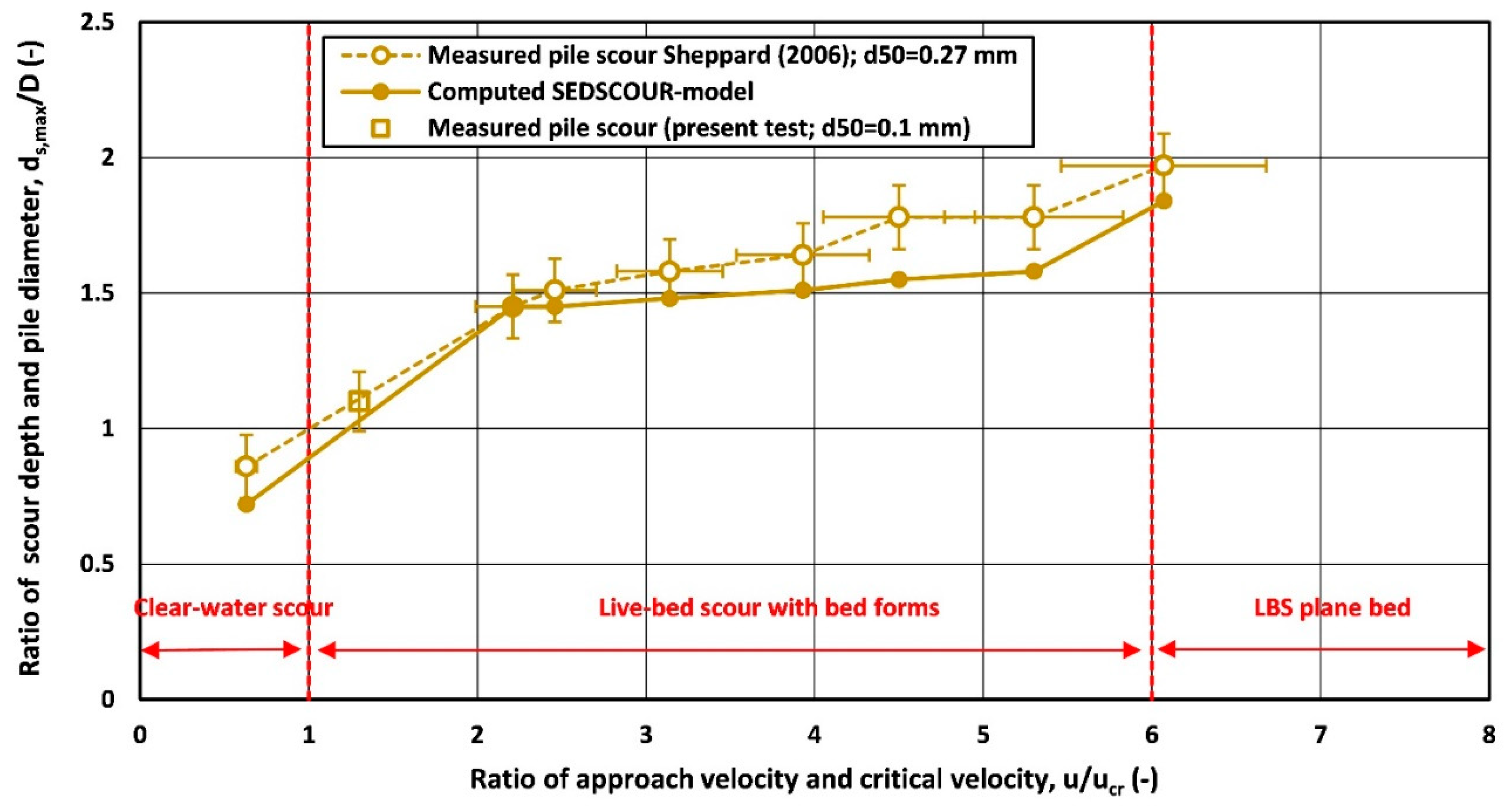
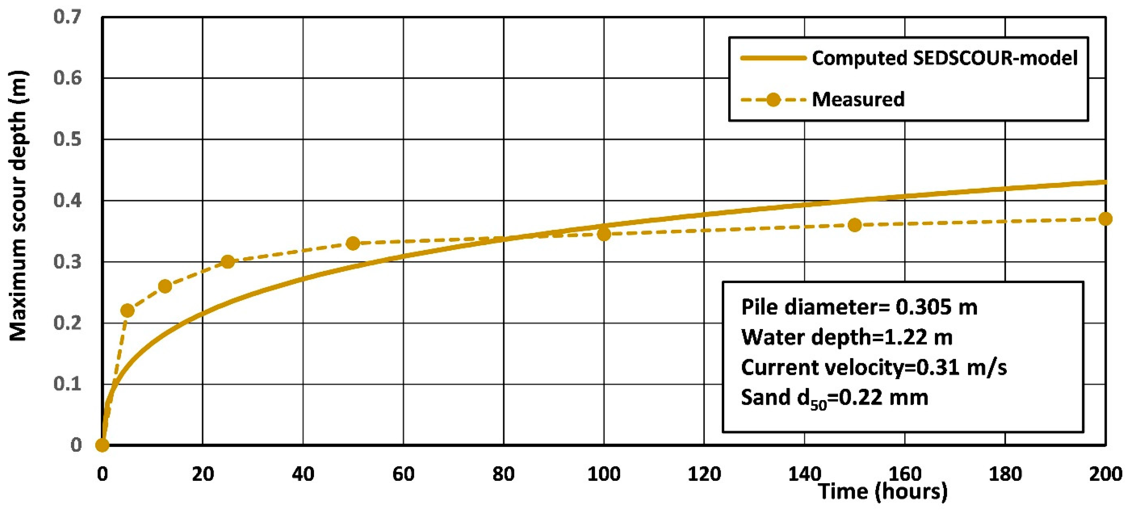
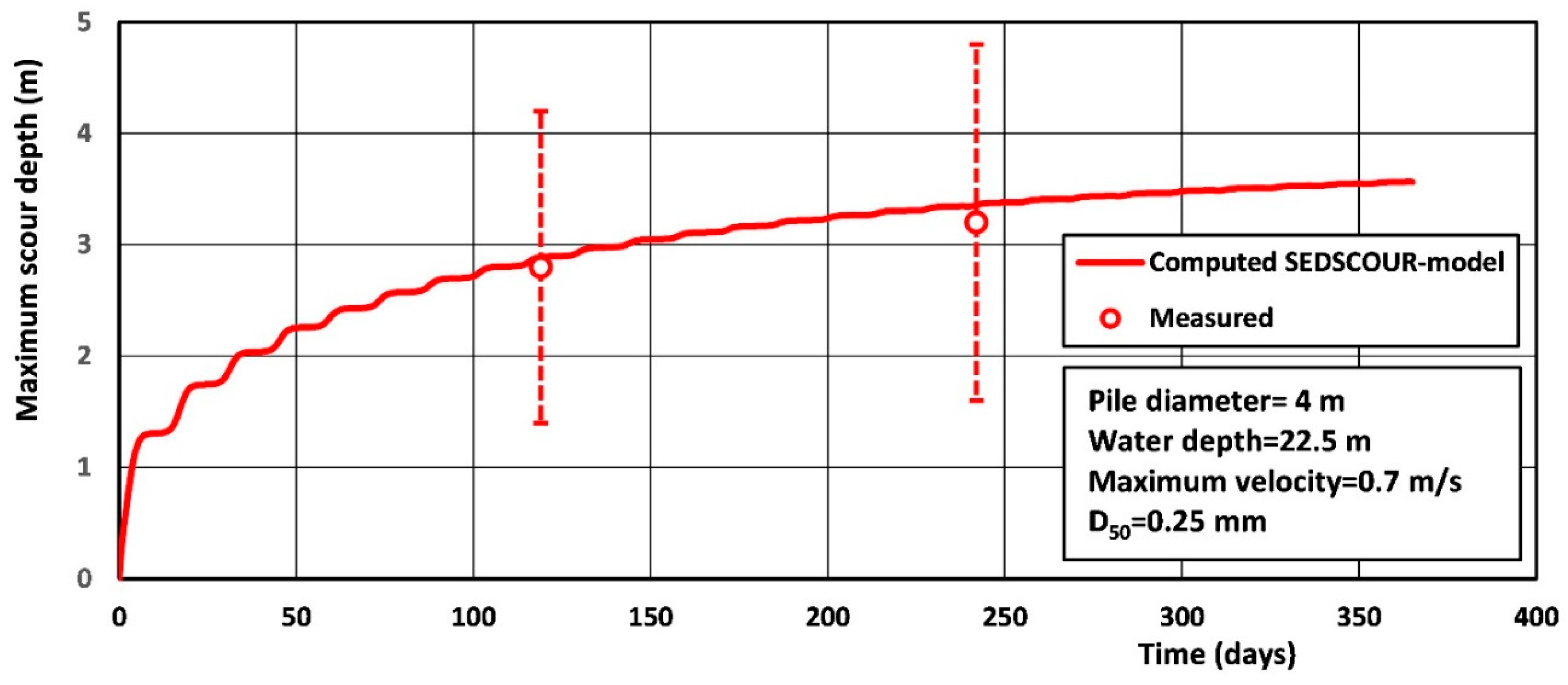
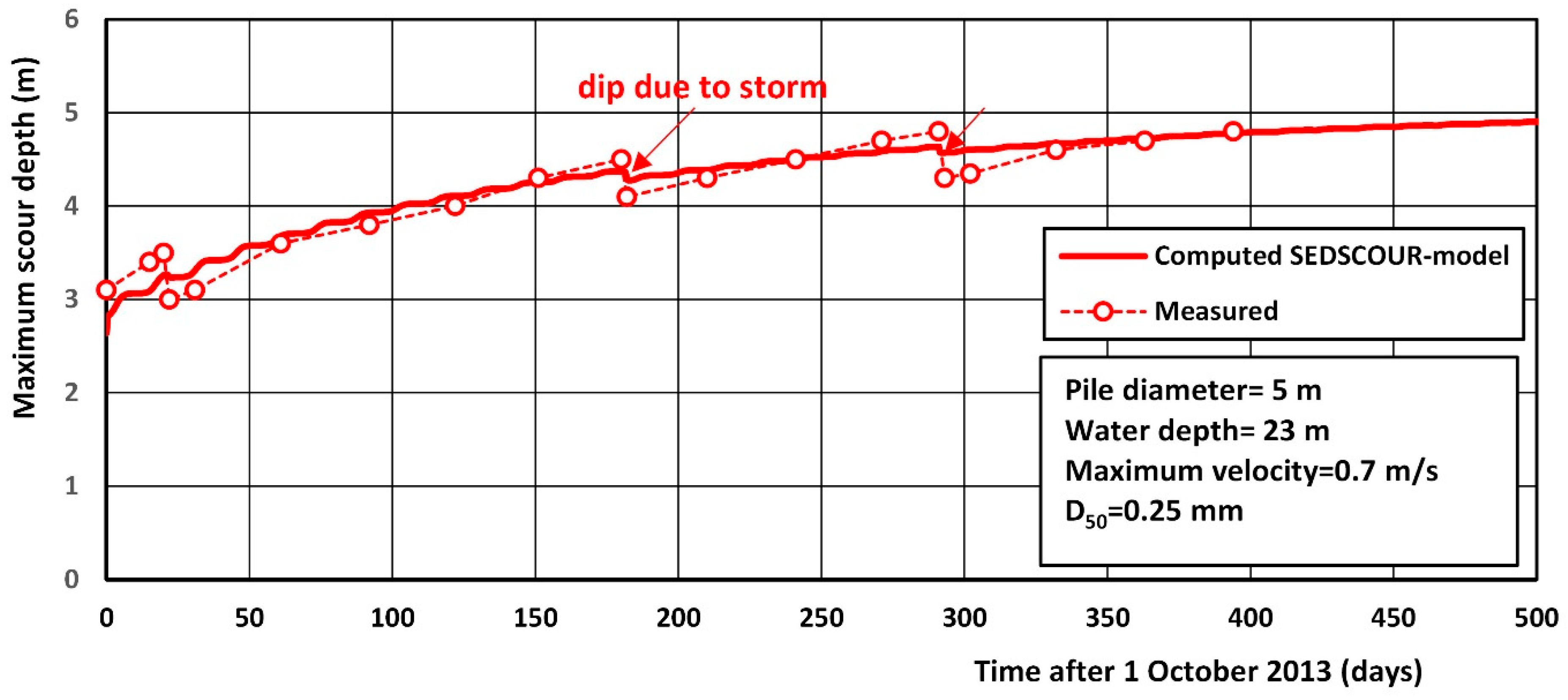
5.3. Free Scour near Monopile; SEDSCOUR-Model Results (Case A to D)

Two laboratory data sets of free scour (without bed protection) and two field cases are considered:

A.

free scour around monopile in flume experiments of Sheppard and Miller [28];

B.

free scour around monopile in flume experiments of Sheppard [29];

C.

free scour around monopiles Q7 wind park (NL) in 2006-2007;

D.

free scour around monopiles windpark Luchterduinen (NL) in 2013.

Case A: Sheppard and Miller [28] measured the scour depth around a monopile in a laboratory flume with a sand bed (d₅₀=0.27 mm, fall velocity=0.03 m/s; u_cr=0.27 m/s, porosity=0.4; sediment density=2650 kg/m³). The water depth was about 0.42 m. The pile diameter was 0.152 m. The approach current velocity was varied in the range of 0.17 to 1.64 m/s. The test with velocity of 017 m/s is a clear-water scour tests (no sediment load in upstream current); the other tests are live-bed scour tests with recirculation of the sediment load. The basic data and model input coefficients are given in Table 3. The velocity increase-coefficient is set to α_u=1.4 for all cases, the turbulence coefficient is in the range of r_o=0.3 to 0.4. The pickup and trapping coefficients are the same for all cases (α_P=1 and α_D=0.5). The measured and computed dimensionless scour depths (d_s,max/D_pile) are shown on the vertical axis of Figure 12. The horizontal axis refers to the ratio of the current velocity and critical velocity for initiation of motion (u/u_cr). The computed values show rather good agreement (about 10% too small) with measured values for all live-bed scour test results, but the computed value is too high (20%) for the clear-water-scour test result.

The time scale is 200 hours for the clear-water scour tests and less than 1 hour for most of the live-bed scour tests.

Figure 12 also shows the maximum scour depth data of the monopile test of the present tests (square symbol; data of Table 2). The results are in good agreement with the other data.

Case B: Sheppard [29] measured the scour around a monopile in a long, wide flume with water depth of 1.22 m above a short sand bed with d₅₀=0.22 mm, fall velocity≅0.025 m/s, critical velocity u_cr≅0.3 m/s, bed porosity=0.3, sediment density=2650 kg/m³. The current velocity was 0.31 m/s. The model settings are given in Table 4.

Figure 13 shows the measured and computed maximum scour depth as function of time. The computed maximum equilibrium scour depth is about 0.43 m, which is somewhat higher (15%) than the measured values of 0.37 m (≅1.2 D_pile). The time scale of the measured equilibrium scour depth is about 50 hours, which is much shorter than that of the computed value of 150 to 200 hours. Most likely, the strong effect of the near-bed horseshoe-type vortices is not sufficiently well represented in the SEDSCOUR-model.

Case C: The offshore wind park Q7 Princess Amalia was built in 2006/2007 at about 20 km off the Dutch coast. The water depths were between 20 and 25 m. The bed consisted of medium fine sand (0.2 to 0.3 mm). The monopiles (diameter of 4.0 m) were exposed to waves and currents for several months without scour protection. The tidal range was about 2 m. The main direction of the tidal current was SSW-NNE. The maximum tidal current during a spring tide was about 0.9 m/s (depth-averaged). The basic data are given by [9].

The measured maximum scour depths of 29 monopiles (without scour protection) were in the range 1.5 to 4.5 m (3±1.5 m), see also Figure 14. The variation is most likely related to variations of the hydrodynamic conditions, which are not exactly the same among the piles. The scour extent (radius of longest axis) was about 20 to 30 m. The shape of the scour hole was oval with a length ratio of 1.8 between the main axis (averaged radius 27 m) and the short axis (average radius 15 m). The side slopes of the scour pit were rather mild (1 to 10), which is very different from the steep side slopes often found in laboratory experiments (1 to 2 or 1 to 3). Measured and computed scour depth are shown in Figure 14. The measured values are those of Pile 48 [9]. The model input data are given in Table 5. The neap-spring tidal cycle is represented by a sinusoidal function with maximum (tide-averaged) velocity of 0.7 m/s during spring tide and 0.3 m/s during neap tide. The wave height is set to a value of 1 m (no storms). The agreement between measured and computed scour depths is rather good.

Case D: The wind park Luchterduinen (NL) consisting of 43 monopile foundation structures (D_pile=5 m) was built in 2013 at about 23 km off the Holland Coast between the beach villages of Noordwijk and Zandvoort, The Netherlands [30]. The local bed of medium fine sand (0.2 to 0.3 mm) was about 23 m below MSL. The tidal range was about 2 m. The maximum flood current to NNW was about 0.7 to 0.9 m/s; the maximum ebb current to the SSW was about 0.5 to 0.6 m/s. Wave heights in the winter period were between 2 and 6 m. Two monopile foundations were installed without scour protection to monitor the free scour development. Figure 15 shows the measured scour depth of the unprotected monopile as a function of time. The scour depth gradually increases from about 3 m on 1 October 2013 to about 4.5 m on 1 November 2014 (over period of about 400 days). The measured scour depth shows a pronounced dip around the period with storm waves, which is most likely caused by backfilling process in the deep scour with sand coming from upstream (outside). The scour pit extent was of the order of 25 m (≅5 D_pile). Computed scour depths are also shown in Figure 15. The model input data are given in Table 4. The neap-spring tidal cycle is represented by a sinusoidal function with maximum (tide-averaged) velocity of 0.7 m/s during spring tide and 0.3 m/s during neap tide. The wave height is set to a value of 1 m for daily conditions; three storms with waves gradually increasing from 1 to 6 m and decreasing from 6 to 1 m over a period of 3 days are included (superimposed on the tidal velocities of the neap-spring cycle). The overall agreement between measured and computed scour depths is rather good. The model computes small (underestimated) dips in the scour depth values.

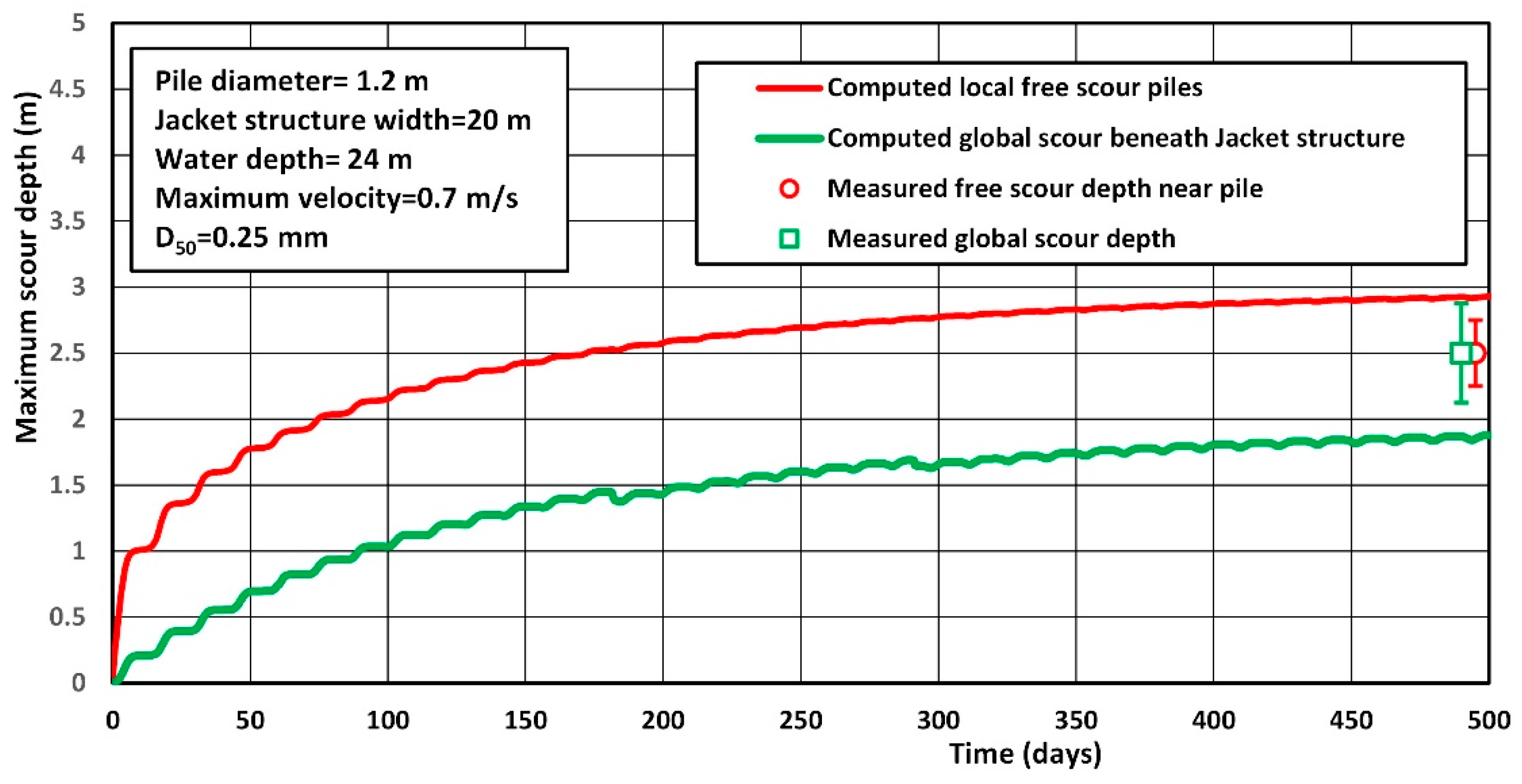
5.4. Free Scour near jacket Structure; SEDSCOUR-Model Results (Case E)

The free scour near the legs of a jacket structure and the overall global scour can also be predicted by the SEDSCOUR-model. One field case is considered herein: Case E which is a jacket structure with four legs installed without scour protection at location L9 in the North Sea, about 30 km north of the island of Texel (The Netherlands) in the summer of 1997 [17]. The bed level was about 24 m below LAT (about 27 below MSL). The jacket structure has four legs with diameter D_J = 1.1 m with a spacing of 20 m and 17 m. The diameter of the piles in the seabed is D_pile = 1.2 m. The bed consisted of fine sand (0.2 to 0.3 mm). Typical depth-averaged peak flow velocities were 0.5 m/s during spring tide and 0.35 m/s during neap tides. The maximum measured wave height and current velocity since installation in 1997 was: H_s = 7.8 m, T_p = 9.8 s and u = 1.0 m/s. Measured maximum global scour depths were in the range of 1.5 to 3 m. The extent of the global scour hole was of the order of 50 m (≅40 D_pile) in all directions. The maximum scour around the foundation pile B2 was found to be about 5 m consisting of global scour and local pile scour. Assuming a global scour depth of 2.5 m (50% based on the data of Table 2), the maximum local pile scour is about 2.5 m (about 2D_pile). The model input data are given in Table 4. Computed scour depth are shown in Figure 16. The neap-spring tidal cycle is represented by a sinusoidal function with maximum (tide-averaged) velocity of 0.7 m/s during spring tide and 0.3 m/s during neap tide. The wave height is set to a value of 1 m (no storms). The maximum computed global scour depth is of the order of 2 m after about 1.5 years. The local maximum scour depth near the pile (D_pile=1.2 m) of the structure is about 3 m after 1.5 years. The total maximum computed scour depth is 2+3=5 m after 1.5 years. The total maximum scour observed scour leg near leg B2 is about 5 m after 3 years (pile scour ≅2.5 m and global scour ≅2.5 m). Hence, computed and measured values are in good agreement, see Figure 16.

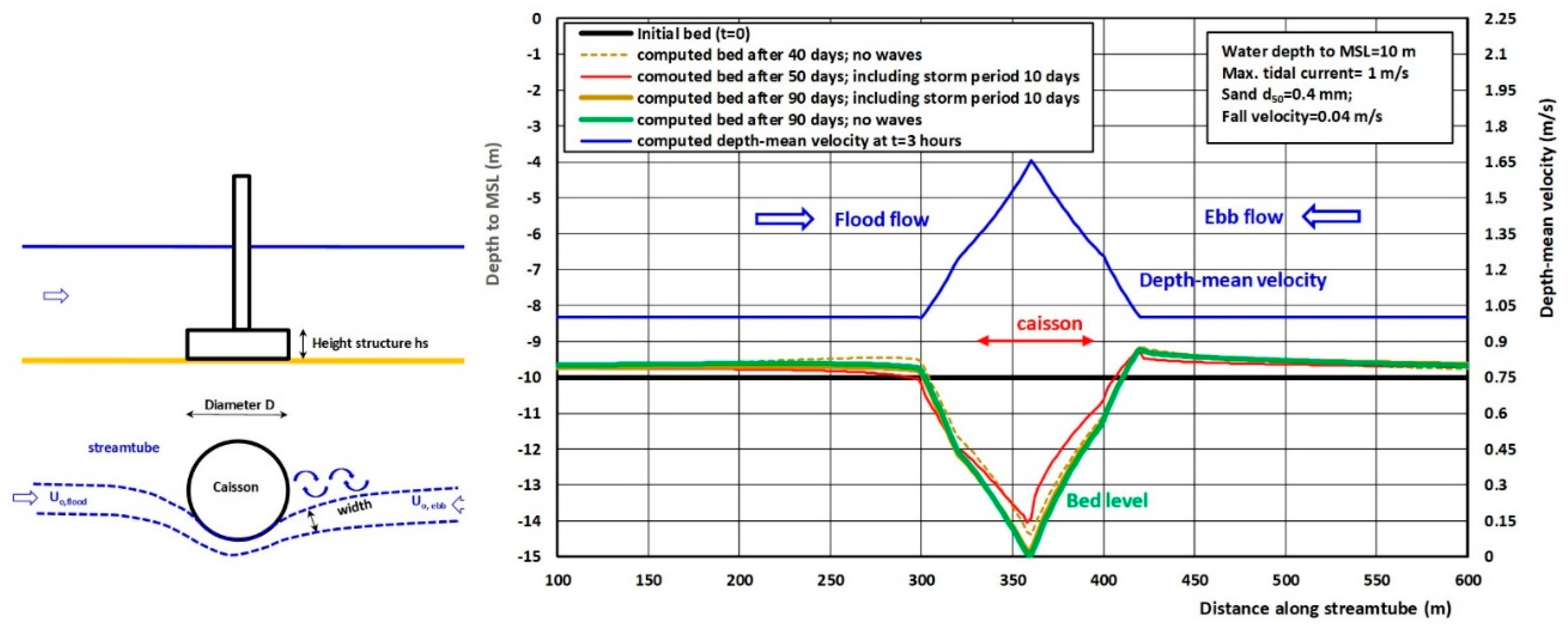
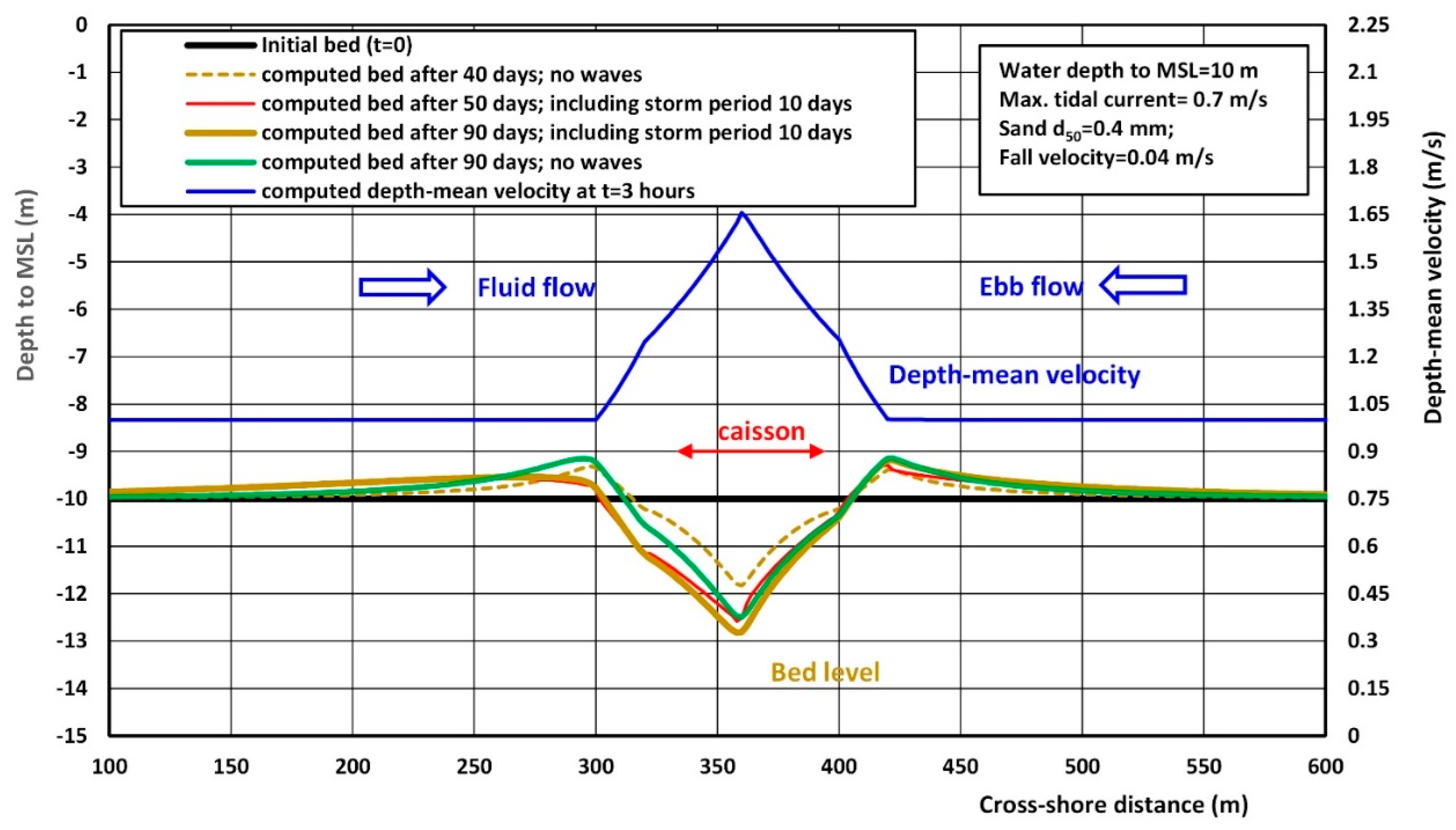
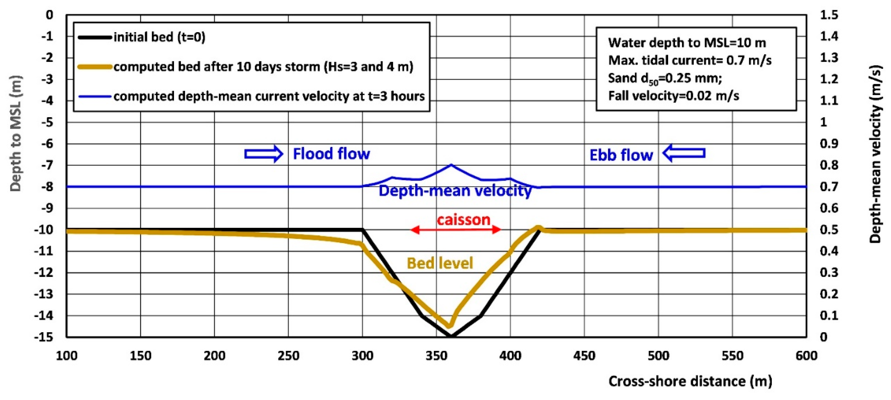
5.5. Free Scour Along Caisson Type Structure; SUSTIM2DV-Model Results (Case F)

5.5.1. General

This example (Case F) considers the scour near a caisson-type structure with diameter of 40 m and a height of 8.8 m. The monopile on top of the structure has a diameter of 11 m. The prediction of scour around the flanks of a large-scale caisson type structure with a monopile on top of it essentially requires the use of a 3D morpho-dynamic model. Given the complexity and long run times of 3D-models, herein a more pragmatic approach is used based on a combination of a depth-averaged flow model (DELFT3D) and a two-dimensional vertical morpho-dynamic model (SUSTIM2DV [23,24]). This latter model can simulate the scour processes and the long-term bed development in a stream tube (Figure 20) along the perimeter of the caisson-structure. The stream tube width is derived from 2DH model results and is assumed to be constant in time.

5.5.2. Computed Flow Field of DELFT3D-Model

The DELF3D-model was operated in 2DH (1 layer) and 3D-mode (8 layers) to compute the flow field. A rectangular computational grid was constructed. The grid was nonuniform in both directions, with a gradual transition in grid cell size, in order to obtain the highest resolution close to the structure. In total, the grid comprises 347 cells in the streamwise direction and 107 cells in the spanwise direction. Accordingly, the grid spans approximately 1600 m and 800 m in either direction, respectively. Close to the structure, the cells have a resolution of 2 m in both directions.

To obtain a unidirectional current in the far-field part of the spatial domain, an open boundary was defined at the upstream boundary where a constant current velocity is prescribed. At the downstream end of the spatial domain, another open boundary was defined where a constant water level was prescribed. At the lateral closed boundaries, a free-slip condition was applied, implying that the tangential shear stress is zero. Basic input parameters are: Chézy-coefficient C=60 m^0.5/s.; k-epsilon model for vertical turbulent viscosity and horizontal large eddy simulation (HLES) for horizontal turbulent viscosity, time step=0.3 s. Figure 17 shows depth-averaged flow velocity vectors for 2DH and 3D mode. The depth-averaged current velocities are quite similar, except for the wake region. Figure 18 shows the flow velocity vectors in the near-bottom layer of the 3D run. The approach velocity in the near-bottom layer is about 0.15 m/s. The distribution of the relative depth-averaged current velocity along the flank of the base structure based on 2DH and 3D model runs is shown in Figure 19 left. It follows that the acceleration computed by the 2DH and 3D models is very similar, based on the depth-averaged current velocity. The maximum increase of the depth-averaged velocity is about 20% with respect to the approach current velocity. Figure 19 right shows the computed relative velocity close to the bottom based on the 3D model run along the structure (black line of inset). Most apparent is that the computed acceleration at this height along the flank is significantly stronger (unearbed,flank≅1.8 unearbed, approach).

Figure 17. Case F: depth-averaged flow field based on 2DH-mode (left) and 3D-mode (right) and HLES;.

Figure 17. Case F: depth-averaged flow field based on 2DH-mode (left) and 3D-mode (right) and HLES;.

depth-averaged approach velocity U_o=0.42 m/s

Figure 18. Case F: flow field in near-bottom layer of 3D model run; U_o=0.42 m/s.

Figure 18. Case F: flow field in near-bottom layer of 3D model run; U_o=0.42 m/s.

Figure 19. Left: depth-averaged flow velocity of 2DH and 3D model runs along structure (black line of inset);.

Figure 19. Left: depth-averaged flow velocity of 2DH and 3D model runs along structure (black line of inset);.

Right: flow velocity 2DH along structure (black line) and 3D in bottom layer along structure (black line)

(u_o=0.42 m/s for depth-averaged flow; u_o=0.15 m/s near-bottom for 3D model; Case F)

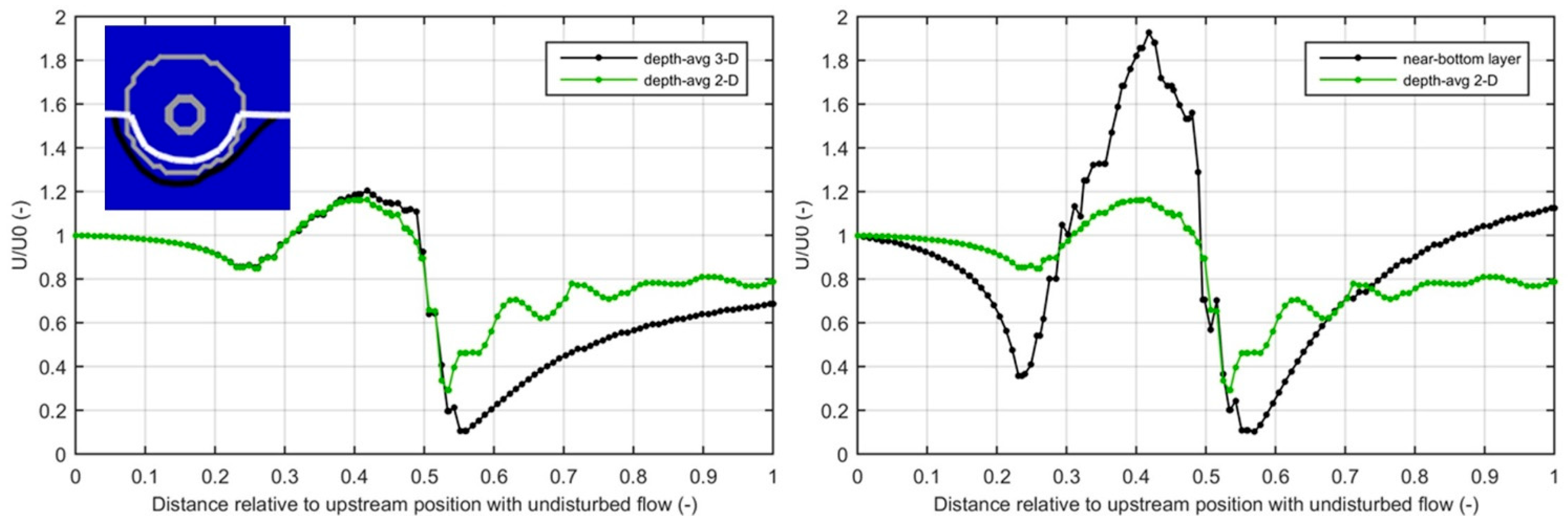
5.5.3. Computed Erosion in Stream Tube along Flank of Caisson

As an example, the sand transport in accelerating and decelerating flow along a caisson structure (diameter D=40 m and height h=10 m; effective water depth=10 m) with a monopile on top of it is considered, see Figure 20. The maximum flow velocity along the flank is assumed to be 1.7 times the upstream approach velocity (u_flank≅1.7u_o ) based on the 3D-results of Figure 19 right. The minimum width of the stream tube at the flank is set to 0.6 of the width at entrance (b_minimum≅0.6b_o). The basic input data are: water depth upstream of trench (10 m to MSL); tidal current with amplitude of 1 m and peak current of 1 and 0.7 m/s; sand with d₅₀=0.4 mm; computation period=90 days; time step =8 s, NZ=25=number of vertical points over the depth.

The computed scour results are shown in Figure 20. The maximum scour depth is about 4.5 m after 40 days (no waves). The maximum scour depth decreases to 4 m after 50 days due to deposition during the storm period of 10 days (H_s=3 and 4 m between t=40 to 50 days). The maximum scour depth increases to 5 m after 90 days due to current (no waves between t=50 and 90 days). Often, it is necessary to install scour protection. The structure may also be placed in a dredged pit with depth of 2 to 3 m to reduce the scour depth. Steel skirts can be attached to the foundation structure to prevent undermining of the caisson structure in conditions with strong flows.

Figure 21 shows the computed scour hole over 90 days for a lower peak tidal flow velocity of 0.7 m/s (in stead of 1 m/s) resulting in a lower sand transport value at peak tidal flow conditions. The maximum scour depth is about 1.8 m after 40 days (tidal flow without waves), which increases to about 2.6 m after 50 days for tidal flow and a storm period of 10 days (t=40 to 50 days) with H_s between 3 and 4 m. The maximum scour depth increases to about 2.8 m after 90 days due to tidal current (no waves between t=50 and 90 days). The maximum scour depth after 90 days is slightly smaller (2.5 m) in conditions without a storm period. The scour on the left slope is lower and the deposition on the left side is somewhat higher.

Figure 22 shows the effect of a storm period of 10 days with H_s between 3 and 4 m on the deposition in the deep scour hole around the base caisson structure with maximum depth of 5 m in a sand bed of d₅₀=0.25 mm. The flow velocity in the deepest part of the scour hole increases due to flow contraction around the structure, but the flow decreases due to flow expansion (larger water depth in scour hole). Overall, the flow velocity increases slightly (10%). The maximum upstream depth-mean velocity at t=3 hours (peak tidal flow) is about 0.7 m/s, which increases slightly to 0.8 m/s. Deposition of sand occurs in the storm period, mostly at the right slope due to higher sand transport during ebb flow when the water depth is smallest. Erosion occurs on the left slope. Thus, deposition prevails in a scour hole during a storm period (Figure 20 and Figure 22). Overall, the computed maximum scour depth near the base caisson structure is in the range of 3 to 5 m, which is of the right order of magnitude based on the physical model study of Sarmiento et al. (2024) [16].

6. Summary and Conclusions

The scour near various offshore structures (monopile, caisson foundation, jacket structure) has been studied by performing laboratory tests in a wide flume and numerical model runs with a semi-empirical model (SEDSCOUR) and a sophisticated 2DV-model (SUSTIM2DV). Measured and computed results have also been compared to scour data from the international Literature. The laboratory test results show that the maximum free scour depth (d_s,max) around a monopile without bed protection is slightly higher than the pile diameter (d_s,max=1.1 D_pile).

The maximum scour depth along the flank of a circular caisson foundation structure is found to be related to the base diameter of the structure (d_s,max≅0.25 D_base). The skirt under the caisson structure should be relatively long, otherwise it may easily be undermined due to erosion causing the tip over of the total structure.

The maximum scour consisting of pile scour and global scour around an open jacket structure standing on 4 piles is found to be much lower than the scour near the other structures (monopile and caisson).

The main cause of the scour near these types of structures is the increase of the velocity along the flanks of the structure (pile, caisson). Detailed velocity measurements showed a significant increase of the depth-averaged velocity up to 40%. The increase of the near-bed velocity may be even higher (up to 70%) based on DELFT3D-model runs resulting in a strong increase of the pickup and transport of sediments and associated erosion.

The measured scour depth values of the physical model tests with the monopile and the open jacket structure of this study are in reasonable agreement with other scour data from the Literature. The dimensionless scour parameters are also in reasonable agreement with measured field scour data of monopiles and jacket structures. Hence, the many available scour data sets are sufficiently reliable to be used for scour predictions of similar structures. It is more difficult to evaluate the measured scour data of a circular caisson foundation. The measured maximum scour depth along the flank of the caisson of the present laboratory tests is much higher (factor 2) than that measured by Sarmiento et al. (2024) [16] for a similar structure, but much lower (factor 2) than some of the test results of Whitehouse (2004) [11] and Tavouktsoglu (2017) [15]. Obviously, the maximum scour depth along a large-scale caisson structure is strongly dependent on the precise geometry and dimensions of the structure and the prevailing flow and sediment conditions. At present stage of research, scour predictions for a circular gravity based structure (GBS) should always be based on the results of physical scale model tests in a laboratory basin in combination with numerical modelling.

Various empirical scour models (relationships) are available for the scour prediction around monopiles and jacket structures. However, many of these models/relationships are based on laboratory scour data only resulting in unreliable time-scale predictions. The semi-empirical SEDSCOUR-model proposed in this paper is based on well-known sediment transport predictors for bed load and suspended load transport in laboratory and field conditions resulting in a reliable time scale prediction, as shown by the successful scour predictions for various laboratory and field cases with monopiles and jacket structures. It has been shown that the SEDSCOUR-model can be used for the reliable prediction of free scour, edge scour and global scour near monopiles and jacket structures in a sandy bed (even with some mud), but not for large scale caisson-type foundation structures.

The prediction of scour along the flank of a caisson structure requires the use of a more sophisticated morpho-dynamic model, preferably a 3D-model operated on a very fine grid. At present stage of computer power, these models cannot be used for realistic long term predictions. Therefore, herein another approach using a detailed 2DV-model with a fine grid along a stream tube following the contour of the caisson was explored. The dimensions of the stream tube can be derived from a 3D-flow model. The SUSTIM2DV-model [22,23] simulates the sediment transport in 50 to 100 points over the depth along the stream tube and can be run at a time-scale of 1 year. An application for a caisson with base diameter of 40 m shows a realistic maximum scour depth of about 5 m on a time scale of a few months. Model runs with storm waves included show that the scour depth is slightly reduced due to sediment deposition in the scour pit during storm, which has also been observed in field conditions (Luchterduinen wind park, The Netherlands).

References

1. Breusers, H.N.C., Nicollet, G. and Shen, H.W., 1977. Local scour around cylindrical piers. J.. Hydr. Res. Vol. 15. [CrossRef]
2. Melville, B.W., 1988. Scour at bridge sites., p. 327-362. Technomic Publishing Company, USA, Civil Engineering Practice, 2.
3. Melville, B.W. and Sutherland, A.J., 1988. Design method for local scour at bridge piers. Journal of Hydraulic Engineering, ASCE, Vol. 114, No. 10. [CrossRef]
4. Kothyari, U.C. et al., 1992. Live-bed scour around cylindrical bridge piers. J. of Hydr. Res., IAHR, Vol. 30 (5). [CrossRef]
5. Melville, B.W., 1997. Pier and abutment scour: integrated approach. Journal of Hydraulic Engineering, Vol. 123 (2). [CrossRef]
6. Lim, S.Y., 1997. Equilibrium clear-water scour around an abutment. J. of Hydraulic Engineering, Vol. 123, No. 3. [CrossRef]
7. Melville, B.W. and Coleman, S.E., 2000. Bridge scour. Water resources Publications. Littleton, Colorado, USA.
8. Cefas, 2006. Scroby sands offshore wind farm; coastal processes monitoring. Cefas Lowestoft Laboratory, UK.
9. Rudolph, D., Raaijmakers, T. and Stam, C.J., 2008. Time-dependent scour development under combined current and wave conditions; hindcast of field measurements. 4th International Conference on scour and erosion, Tokyo.
10. Raaijmakers, T.C., Van Velzen, G. and Riezebos, H.J., 2014. Dynamic scour prediction for offshore monopiles. Proceedings of 7th Int. Conf. Scour and Erosion. 2-4 December 2014, Perth, Australia.
11. Whitehouse, R.S.J., 2004. Marine scour at large foundations. 2snd Int.l Conference on Scour and Erosion, Singapore.
12. Whitehouse, R., Harris, J., Sutherland, J. and Rees, J., 2008. An assessment of field data for scour at offshore wind turbine foundations. Fourth International Conference on scour and erosion, Tokyo.
13. Whitehouse, R., Harris, J. and Sutherland, J., 2012. Evaluating scour at marine gravity structures. HR Wallingford; ICE-Maritime Engineering, Vol. 164, 143-157.
14. Simons, R.R., Weller, J. and Whitehouse, R.J.S. 2009. Scour development around truncated cylindrical structures. Coastal Structures 2007, Proceedings of the 5th Coastal Structures International Conference, CSt07, Venice, Italy, 2-4 4 July 2007, (Eds) Franco, L., Tomasicchio, G.R. and Lamberti, A., 1881-1891. World Scientific.
15. Tavouktsoglu, N.S., 29017. Scour and scour protection around offshore gravity-based foundations. Doctoral Thesis, University College, London,UK.
16. Sarmiento, J., Guanche, R., Losada, I.J. and Serna, J. 2024.Experimental analysis of scour around an offshore wind gravity base foundation. Ocean Engineering Vol. 308, Doi.org/10.1016/j.oceaneng.2024.118330. [CrossRef]
17. Rudolph, R., Bos, K.J., Luijendijk, A.P., Rietema, K. and Out, J.M.M., 2004. Scour around offshore structures; analysis of field measurements, Deltares, Delft, The Netherlands.
18. Bolle, A., de Winter, J., Goossens, W., Haerens, P. and Dewaele, G., 2012. Scour monitoring around offshore jackets and gravity based foundations. In Proceedings of the Sixth International Conference on Scour and Erosion, ICSE 6, Paris, France, 27–31 August 2012.
19. Baelus, L., Bolle, A. and Szengel, V., 2018 Long term scour monitoring around offshore jacket foundations on a sandy seabed. In Proceedings of the Ninth International Conference on Scour and Erosion, ICSE 9, Taipei, Taiwan, 5–8 November 2018.
20. Welzel, M., Schendel, A., Schlurmann, T. and Hildebrandt, A., 2019. Volume-based assessment of erosion patterns around a hydrodynamic transparent offshore structure. Energies, Vol. 12. [CrossRef]
21. Zhang, J., Zhang, P., Guo, Y., Ji, Y. and Fu, R., 2025. Large eddy simulation of the flow field characteristics around a jacket foundation under unidirectional flow actions. Ocenan Engineering, Vol. 137. [CrossRef]
22. Chambel, J., Fazeres-Ferradosa, T., Miranda, F., Bento, A.M, Taveiro-Pinto, F. and Lomonaco, P., 2024. A Comprehensive Review on Scour and Scour Protections for Complex Bottom-Fixed Offshore and Marine Renewable Energy Foundations. Ocean Engineering, Vol. 304 (8). [CrossRef]
23. Van Rijn, L.C., Meijer, K., Dumont, K. and Fordeyn, J.,2024a. Practical 2DV modelling of deposition and erosion of sand and mud in dredged channels due to currents and waves. Journal of Waterway, Port, Coastal and Ocean Engineering. [CrossRef]
24. Van Rijn, L.C., Meijer, K., Dumont, K. and Fordeyn, J., 2024b. Simulation of sand and mud transport processes in currents and waves by time-dependent 2DV model. International Journal of Sediment Reserch. [CrossRef]
25. Van Rijn, L.C., 1993, 2012. Principles of sediment transport in rivers, estuaries and coastal seas. Aqua Publications, Amsterdam, The Netherlands. Available online: www.aquapublications.nl.
26. Van Rijn, L.C., 2007a. Unified view of sediment transport by currents and waves, I: Initiation of motion, bed roughness, and bed-load transport. Journal of Hydraulic Engineering, Vol. 133 (6),649-667. [CrossRef]
27. Van Rijn, L.C., 2007b. Unified view of sediment transport by currents and waves, II: Suspended transport. Journal of Hydraulic Engineering, Vol. 133 (6), 668-389. [CrossRef]
28. Sheppard, D.M. and Miller, W., 2006. Live-Bed local pier scour experiments. Journal of Hydraulic Engineering, ASCE, Vol. 132, No.7 , 635-642. [CrossRef]
29. Sheppard, D.M., 2003. Large scale and live bed local pier scour experiments (phase 1). Final Report Florida Department of Transportation FDOT, USA.
30. Deltares 2017. Scour and scour mitigation; Hollandse Kust Zuid Wind Farm Zone. Delft, The Netherlands.
Figure 10. Plan view and cross-section of scour pit due to tidal flow.
Preprints 143052 g010
Figure 11. Scour downstream of a hard structure (obstacle) on the sea bed.
Preprints 143052 g011
Figure 12. Case A: scour depth as function of current velocity; tests Sheppard and Miller [28].
Preprints 143052 g012
Figure 13. Case B; measured and computed scour depth as function of time; test Sheppard (2003).
Preprints 143052 g013
Figure 14. Case C: measured and computed free scour depth as function of time; Q7 windpark (NL).
Preprints 143052 g014
Figure 15. Case D: measured and computed free scour depth as function of time; Luchterduinen wind park (NL).
Preprints 143052 g015
Figure 16. Case E: Computed scour depth as function of time; Jacket structure L9, North Sea (NL).
Preprints 143052 g016
Figure 20. Case F: flow and scour around caisson (diameter= 40 m; height= 10 m ; seabed 0.4 mm sand).
Preprints 143052 g020
Figure 21. Case F: flow velocity and scour along stream tube ; maximum velocity= 0.7 m/s ; d50=0.4 mm.
Preprints 143052 g021
Figure 22. Case F: flow velocity and scour along stream tube; maximum upstream velocity= 0.7 m/s ; d50=0.25 mm.
Preprints 143052 g022