
Submitted:
13 April 2025
Posted:
15 April 2025
You are already at the latest version
Abstract
Inflammatory bowel disease (IBD) is a chronic inflammatory condition of the gastrointestinal tract characterized by the deregulation of immuno-oncology markers. IBD includes ulcerative colitis and Chron disease. Chronic active inflammation is a risk factor for the development of colorectal cancer (CRC). Deep learning is a form of machine learning that is applicable to computer vision, and it includes algorithms and workflows used for image processing, analysis, visualization, and algorithm development. This technical note of data descriptor and methods type describes a dataset of histological images of ulcerative colitis, CRC (adenocarcinoma), and colon control. The samples were stained with hematoxylin and eosin (H&E), and immunohistochemically analyzed for LAIR1 and TOX2 markers. The methods used for collecting, processing, and analyzing scientific data using convolutional neural networks (CNNs), where the dataset can be found, and information about its use is also described. This note is a companion to the DOI: 10.3390/cancers16244230.
Keywords:
ulcerative colitis
; colorectal cancer
; adenocarcinoma
; artificial intelligence
; deep learning
; convolutional neural network
; transfer learning
; TOX2
; LAIR1
; H&E
; whole-slide images
; ResNet-18
1. Summary
1.1. Background of Ulcerative Colitis
Inflammatory bowel disease (IBD) is a chronic inflammatory condition of the gastrointestinal tract with systemic repercussions that is characterized by relapsing and remitting episodes of inflammation [1,2]. IBD includes 2 types: ulcerative colitis, which affects the colon, and Chron disease, which can affect any part of the gastrointestinal tract from the mouth until the perianal area [1,2,3,4,5,6,7,8,9].
The causes and pathogenesis of IBD are unclear. However, it appears to be a combination of factors from the environment, including the microbiome [10,11], genetic susceptibility [12,13], and immune system (both systemic and gut) [13,14,15,16]. The prevalence of IBD has increased globally in recent decades, particularly in industrialized countries [17,18,19,20,21]. Clinical risk factors include smoking [22], low physical activity, low fiber intake, high fats, and low vitamin D [23], sleep deprivation, previous acute gastroenteritis, antibiotic use, and early life exposures [24].
In normal and healthy conditions, the intestinal barrier is maintained by the mucus layer and epithelial cells, which create bonds using tight junctions. This barrier is supported by the presence of IgA and several antimicrobial factors. The immune response is initiated by dendritic cells, which acquire, process, and present antigens to B and T lymphocytes [25]. The cause of ulcerative colitis is still not completely understood. Ulcerative colitis is associated with mucosal barrier damage, microflora alteration, and an uncontrolled immune reaction. Several subsets of CD4-positive T cells are believed to participate in the pathogenesis of UC, including Th1, Th2, Th9, Th17, Th22, TFh lymphocytes, and Tregs [26,27].Th9 are associated with enterocyte apoptosis and inhibit mucosal healing [25,28]. IL-13 and NK/T cells are also involved in epithelial injury [25]. Innate immune cells contribute to cytokine production and continuous inflammation [14,15,29]. Injury of the mucosa is associated with dysbiosis [30], which is defined by an alteration of the composition of the mucosa, with changes of the diversity, increased potentially pathogenic bacteria, and reduced beneficial bacteria [31]. Figure 1 and Figure 2 show examples of ulcerative colitis and IHC of the cells of the microenvironment involved in the pathogenesis.
The disease activity of ulcerative colitis is being recorded to properly treat patients and perform clinical trials. Usually, the severity is classified as mild, moderate, or severe. The available classifications include the Mayo [32], Montreal [33], Truelove, and Witts classifications [34]. The grade of mucosal inflammation can be assessed using endoscopy to record the degree of mucosal ulceration and the extent of disease. This can be graded using the Mayo score [32] and Baron score. The degree of histological severity can be evaluated using the Geboes score [35].
Microscopic (histologic) evaluation of ulcerative colitis shows active chronic colitis in patients with untreated disease. Disease activity is defined by neutrophil infiltration of the lamina propria, cryptitis, crypt abscess, and ulceration. The inflammation is limited to the mucosa and submucosa. Compared with Crohn disease, this condition is associated with a lack of transmural inflammation, granuloma, and fissuring ulcers. Dysplasia may be present in patients with long-term disease [36,37,38].
Disease activity can be evaluated using various parameters. Inactive disease lacks neutrophils. If the activity affects less than 50% of the mucosa, it is called mild. When it is >50% and there are crypt abscesses, it is called moderate. Finally, severe activity is characterized by surface ulcerations and erosion [39].
The first-line therapy for the induction and maintenance of remission of mild to moderate UC is 5-aminosalicylic acid [40]. The initial therapy for ulcerative colitis is topical mesalamine, which is available as a suppository or enema, and it is recommended for ulcerative proctitis or proctosigmoiditis. If topical mesalamine is not tolerated, an alternative therapy is topical glucocorticoids (i.e. hydrocortisone). A combination of 5-ASA and rectal mesalamine may be used for left-sided or extensive colitis. The 5-ASA formulations include mesalamine, sulfasalazine, and diazo-bonded 5-ASA. Patients who do not respond may subsequently be treated with glucocorticoids such as budesonide, which may escalate to prednisone or biological agents (anti-TNF, anti-integrin, anti-IL12/23, S1P modulators, JAK inhibitors) [40,41,42,43]. Patients who do not respond to oral glucocorticoids may require intravenous glucocorticoids. In some cases, surgery is performed [40,41,42,43]. Fecal microbiota transplantation is also available [44].
1.2. Background of Colorectal Cancer
Colorectal cancer (CRC) is a common disease characterized by environmental and genetic factors. It is the third most frequently diagnosed cancer worldwide [45]. There are several factors associated with early onset of CRC, including hereditary syndromes (familial adenomatous polyposis and Lynch syndrome), metabolic dysregulation, history of CRC in first-degree relative; alcohol consumption, lack of regular use of nonsteroidal anti-inflammatory drugs (NSAIDs), and vitamin D intake. Other known risk factors of CRC include inflammatory bowel disease (ulcerative colitis and Crohn disease), abdominopelvic radiation, obesity, diabetes mellitus, insulin resistance, red and processed meat, and tobacco [46,47,48,49]. The diagnosis is usually made by colonoscopy, and treatment includes surgical resection, adjuvant chemotherapy, and postoperative radiation therapy [46]. Adenocarcinoma is the most common histological subtype of CRC. Adenocarcinoma is a glandular neoplasm. Most CRC cases are moderately differentiated with simple, complex, or slightly irregular tubules and loss of nuclear polarity. The glands are often cribriform, with necrosis, inflammatory cells, and marked desmoplasia [50,51,52] (Figure 3).
1.3. Background of Computer Vision for Deep Learning Image Classification
Image processing involves the algorithms and workflows of image processing, analysis, visualization, and algorithm development. Computer vision workflows [53] with deep learning include several types of functions, such as image classification, object detection, and instance segmentation, automated visual inspection, semantic segmentation, and video classification [54,55,56].
A pretrained neural network that has already learned how to extract the characteristics of natural images can be used as a starting point to handle new images. Using a pretrained image classification network [57], the learning time is shorter, and training is usually easier. The transfer learning process takes layers from an already trained neural network and calibrates the parameters on a new dataset [54,55,56,58,59,60,61,62,63,64,65]. The analysis includes a series of steps, including preprocessing the data, import pretrained networks from platforms such as TensorFlow 2 [66], TensorFlow-Keras [67], Pythorch [68], and ONNX [69], building the network, selecting training options, improving the network performance by tuning hyperparameters, visualizing and verifying network behavior during and after training, and exporting the network to other platforms if necessary[54,55,56,58,59,60,61,62,63,64,65].
The most important features of a neural network are accuracy, speed, and size. A good neural network is characterized by being fast and having good performance (i.e. accurate). Neural networks that are accurate in ImageNet can be used to classify other images using transfer learning or feature extraction. The best examples of neural networks, the best examples are GoogLeNet, ResNet-18, NobileNet, ResNet-50, ResNet-101, and Inception-v3 [56]. Figure 4 shows the general design of the CNN, and Figure 5 shows the original RestNet-18 architecture [70].
1.4. Dataset and Research Project Description
Ulcerative colitis is a chronic inflammatory bowel disease associated with a high risk of colorectal cancer. This study used convolutional neural networks and computer vision to classify histological images of ulcerative colitis, colorectal cancer (adenocarcinoma), and colon control.
The series included 35 patients with ulcerative colitis, 18 with colorectal cancer, and 21 with colon control. Hematoxylin and eosin (H&E) glass slides were converted into high-resolution digital data by high-speed scanning. The whole-tissue slides were split into image patches of 224×224 pixels at 200× magnification and 150 dpi, and the ResNet-18 network was retrained to classify the 3 types of diagnosis. This transfer learning experiment also used other pretrained CNNs for performance comparison, and the gradient-weighted class activation mapping (Grad-CAM) heatmap technique was used to understand the classification decisions.
Additionally, immunohistochemical analysis of 2 new immuno-oncology markers, LAIR1 and TOX2 were analyzed in ulcerative colitis to differentiate between mesalazine-responsive and steroid-requiring patients. LAIR1 an inhibitory receptor that plays a constitutive negative regulatory role in the cytolytic function of natural killer (NK) cells, B lymphocytes and T lymphocytes [71,72,73]. TOX2 is a new marker similar to PD-1 in the coinhibitory pathway [71,74].
Statistical analyses showed that steroid-requiring ulcerative colitis was characterized by higher endoscopic Baron and histologic Geboes scores and LAIR1 expression, and lower TOX2 expression in isolated lymphoid follicles. The CNN managed to classify the 3 diagnoses with >99% accuracy, and the Grad-CAM confirmed which parts of the images were relevant for the classification. In conclusion, the study proposed that CNNs are essential tools for deep learning image recognition.
These results were published as preprints [75].
This paper is a companion manuscript of the recently published article “Ulcerative Colitis, LAIR1 and TOX2 Expression, and Colorectal Cancer Deep Learning Image Classification Using Convolutional Neural Networks” published in Cancers 2024, 16, 4230. https://doi.org/10.3390/cancers16244230.
2. Data Description
The dataset contains image patches of ulcerative colitis, colorectal cancer, and colon control. The image patches were split from whole-tissue images and had a size of 224 × 224 × 3. The original magnification of the images was 200× and a dpi of 150. The image patches are anonymized. After splitting the images, the patches were filtered. The criteria were as follows: (1) image patches of only 243×243 size; (2) image patches of more than 5-31 KB that contain tissue at least 20-30% of viable tissue; (3) image patches with diagnostic areas; (4) image patches without artifacts, including broken tissue, folded areas, incorrectly stained tissue, and smashed/crushed tissue. Steps 3 and 4 were manually curated by a pathology specialist (MD PhD).
The investigations were carried out according to the Declaration of Helsinki (website: https://www.wma.net/policies-post/wma-declaration-of-helsinki/; last accessed on December 12, 2024). Approval from an ethics committee was obtained before undertaking the research (protocol code IRB14R-080, IRB20-156, and 13R-119).
3. Methods
3.1. Formalin Tissue Fixation and Paraffin Embedding
Samples were fixed and embedded for long-term storage and immunostaining using fixatives to preserve tissues. The protocol included neutral buffered formalin, 80% alcohol, 95% alcohol, 100% alcohol, xylene, and paraffin pellets. Processing was performed using a HistoCore Peloris 3 premium tissue processing system (#13B2X10268PELOR3, Leica Biosystems K.K., Tokyo, Japan) (Figure 6).
The processed tissue was embedded in paraffin, forming paraffin blocs ready for sectioning using a tissue embedder (Tissue-Tek® TEC™ 6 Embedding Console System, Sakura Finetek Japan Co., Ltd., Tokyo, Japan) (Figure 7).
3.2. Sectioning of Paraffin-Embedded Tissue
Paraffin blocks were trimmed at 2μm using a Yamato REM-710 microtome (Yamato Kohki Industrial Inc., Saitama, Japan) (Figure 8). The paraffin ribbons were placed in 40-50 warmed water bath and mounted onto slides. The sections were later air dried and baked 45-50 ºC in an oven overnight.
3.3. Hematoxylin and Eosin (H&E) Staining
H&E staining is widely used in histological and cytological applications, both in fixed paraffin-embedded and frozen tissue sections. Hematoxylin produces an intense blue staining of the nuclei. Eosin stains the cytoplasm, collagen, muscle, and erythrocytes in light pink/rose. A standard H&E staining protocol includes deparaffinizing with xylene, rehydrating in decreasing concentrations of alcohol (100%, 90%, 80%, 70%, and distilled water), staining with hematoxylin, differentiating, bluing, eosin, dehydration, clearing, and coverslipping. Staining was performed using an automated slide stainer, a Tissue-Tek Prisma® Plus (Sakura Finetek Japan Co., Ltd.,) (Figure 9).
Glass coverslipping of histopathological slide sections was performed using a Tissue-Tek® Glas™ g2 Glass Coverslipper (Sakura Finetek Japan Co., Ltd.).
3.4. Score Evaluation
The endoscopic scores for chronic inflammatory bowel disease were evaluated using the Baron Score, which classifies mucosal changes into 4 grades: grade 0 (normal); grade 1 (abnormal non-hemorrhagic), 2 (moderately hemorrhagic), and 3 (severely hemorrhagic).
Ulcerative colitis histological assessment was performed using the Geboes score: grade 0 (no abnormality), grade 1 (chronic inflammatory infiltrate), grade 2 (lamina propria neutrophils and eosinophils), grade 3 (neutrophils in epithelium), and grade 4 (crypt destruction) (Figure 10).
3.5. Immunohistochemistry
The immunohistochemistry of LAIR1 and TOX2 was performed using a Bond-Max fully automated immunohistochemistry and in situ hybridization staining system following the manufacturer’s instructions (Leica Biosystems K.K.) (Figure 11).
Visualization of the primary antibody bound to the tissue sections was performed using BOND Polymer Refine Detection (DS9800, Leica Biosystems K.K.). The BOND staining mode was single, i.e. a single marker and chromogen were applied to a single slide. Bond Polymer Refine Detection is a biotin-free, polymeric horseradish peroxidase (HRP)-linker antibody conjugate system for the detection of tissue bonding mouse and rabbit antibodies. This detection avoids the use of streptavidin and biotin; as a result, nonspecific staining is reduced.
The protocol sequence was the following: preparation (removal of wax using BOND Dewax Solution, 100% alcohol, and wash solution), heat-induced epitope retrieval (HIER; using BOND Epitope Retrieval ER2 solution), protein block (optional animal-free blocking solution), probe application, probe removal (wash solution), post-primary mouse linker, secondary detection (refine detection kit polymer), visualization (refine detection mixed DAB), and counterstain (hematoxylin). In summary, the staining protocol included the following steps: marker, post primary, polymer, mixed DAB, and BOND-PRIME hematoxylin.
Coverslipping was achieved using a Leica CV5030 fully automated glass coverslipper (Leica Biosystems K.K.) (Figure 12).
The primary antibody targeted the leukocyte-associated immunoglobulin-like receptor (LAIR1/CD305) created by the Monoclonal Antibodies Core Unit, located at the Spanish National Cancer Research Center (CNIO: Centro Nacional de Investigaciones Oncologicas; C/ Melchor Fernandez Almagro, 3, E-28029 Madrid, Spain). LAIR1 is a rat monoclonal antibody, clone JAVI82A, antigen used: RBL-1-LAIR1-MYCDDK transfected cells and last booster with LAIR1 recombinant (Gln22-His163, with a C-terminal 6-His tag); isotype IgG2a; reactivity, human; localization, membrane.
The primary antibody TOX2 targeted the TOX High Mobility Group Box Family Member 2 and was also developed by CNIO. Properties: clone name TOM924D, rat monoclonal, IgG2b K, antigen HIS-SUMO-hTOX2-Strep-tag2 full-length protein, human reactivity, nuclear localization.
Rabbit Anti-Rat IgG Antibody (H+L), Mouse Adsorbed, Unconjugated (#AI-4001-.5, Vector Laboratories, Inc., Newark, CA 94560, United States) was used as a linker between primary antibodies and BOND Polymer Refine Detection.
The immunohistochemistry of both antibodies was first tested in reactive lymphoid tissue (tonsils) and small and large intestinal tissue controls. Four examples of biopsies of the colon of ulcerative colitis stained with TOX2 and LAIR1 and with high infiltration of positive cells are shown in Figure 13, Figure 14, Figure 15 and Figure 16.
Before digitalization, the H&E and immunohistochemical slides were visualized using an Olympus upright microscope for quick evaluation and quality control purposes (Olympus BX63, Olympus K.K., Hachioji, Tokyo, Japan) (Figure 17).
3.6. Whole-Slide Imaging
Whole-slide imaging was performed using a Hamamatsu NanoZoomer S360 scanner (Hamamatsu Photonics K.K., Hamamatsu City, 431-3196, Japan) that rapidly scanned glass slides to convert them to digital data, NZAcquire 1.2.0 software (Hamamatsu Photonics K.K.), and a Dell Precision 5820 Tower equipped with an Intel(R) Xeon(R) W-2135 CPU @ 3.70 GHz 3.70 GHz, 32.0 GB RAM, 64 bits workstation system. The operating system was Windows 10 Pro for Workstations (version 1803, build 17134.1) (Figure 18).
The acquisition method was performed following the manufacturer’s instructions. The scan was batch scan-type, at 400× magnification, and single z stack. The number of focus points was defined automatically using NZAcquire software (Figure 19).
3.7. Digital Image Quantification
Conventional immunohistochemical analysis was performed using digital image quantification with Fiji software, as previously described [76,77,78,79]. In summary, quantification was performed in the blue stack, min and max thresholds were set, pixels were measured, and percentages were calculated (Figure 20).
3.8. Image Classification using CNNs
A convolutional neural network (CNN) was designed based on transfer learning from ResNet-18; and trained to classify the 3 types of image patches; ulcerative colitis (n= 9,281), colon control (n=12,246), and colorectal cancer (n=63,725). The CNN was designed in MATLAB (R2023b, update 9, 23.2.0.2668659). The CNN was also trained to differentiate between mesalazine-responsive and steroid-requiring ulcerative colitis based on H&E, LAIR1, and TOX2 staining (Figure 21 and Figure 22).
The data were partitioned into a training set (70% of the image patches) to train the network, a validation set (10%) to test the performance of the network during training, and a test set (20%) as a holdout (new data) to test the performance on new data.
The arrangement of the images was randomized to ensure that the CNN learned the classes at an even rate. Transfer learning, which involves reusing and adjusting a pretrained network, was performed on ResNet-18. For this purpose, the fully connected and classification layers of ResNet-18 were deleted and replaced with new layers. These new layers had an output size of 2. The training did not employ the augmentation technique. To avoid overfitting, the initial learning rate was set to 0.001. The maximum number of epochs was five [75].
Data normalization was applied to the input images. A detailed description of the data normalization process is provided in Appendix Table A3 [80,81].
The trained network was characterized by 71 layers. The first layer was the “ImageInputLayer”, and the last one the “ClassificationOutputLayer” (Figure 23). The parameters are listed in Table 3.
The code used is shown in Table A4 in the Appendix
In the analysis setup, the image patches of the 3 diagnoses were pooled in 3 different folders. The content of each folder was then split into training, validation, and testing sets. As a result, no image patches were repeated in different folders. Nonetheless, some researchers believe that this strategy could lead to information leakage. Therefore, an additional and independent test set of 10 cases of colorectal cancer (adenocarcinoma) was used to confirm the performance of the trained CNN. Each patient was analyzed independently [75].
Of note, other types of CNNs were tested in this study. The LAIR1 and TOX2 biomarkers were included in the CNN training in an independent analysis of H&E staining. A differentiation between steroid-requiring (SR) and mesalazine-responsive ulcerative colitis using LAIR1 and TOX2 immunohistochemistry.
The performance parameters were the following: accuracy, precision, recall, F1 Score, specificity, and false positive rate.
The performance of ResNet-18 was compared to that of other CNNs under the same experimental conditions, including DenseNet-201, ResNet-50, Inception-v3, ResNet-101, ShuffleNet, MobileNet-v2, NasNet-Large, GoogLeNet-Places365, VGG-19, EfficientNet-b0, AlexNet, Xception, VGG-16, GoogLeNet, and NasNet-Mobile.
3.9. Computational Requirements
All analyses were performed using a desktop computer equipped with an AMD Ryzen 9 7950X CPU, 128 Gb of RAM (Crucial Desktop DDR5-4800 UDIMM 1.1V CL40, CT2K32G48C40U5 x2), and an Nvidia GeForce RTX 4090 graphics card (ASUS ROG Strix GeForce RTX® 4090 OC Edition 24GB GDDR6X). The specifications of the GPU were 16384 Nvidia Cuda® cores, 4th Generation 1321 AI TOPS Tensor cores, 2.23 GHz base and 2.52 GHz boost clock, 24 GB GDDR6X memory, 384-bit memory interface width, Ada Lovelace architecture (Figure 24).
4. Results
This paper of Methods type is a companion manuscript to a recently published article entitled “Ulcerative Colitis, LAIR1 and TOX2 Expression, and Colorectal Cancer Deep Learning Image Classification Using Convolutional Neural Networks”. Published in Cancers (Basel); Published 2024 Dec 19. doi:10.3390/cancers16244230 [75].
In summary, steroid-requiring ulcerative colitis was characterized by higher endoscopic Baron and histologic Geboes scores, higher LAIR1 immunohistochemical expression in the lamina propria, and lower TOX2 in the isolated lymphoid follicles (ILFs). The CNN successfully classified ulcerative colitis, colorectal cancer, and colon control with high performance. The classification was also validated using an independent test sample.
5. Discussion
Artificial Intelligence (AI) is the science and engineering that allows computers and machines to simulate human learning and problem solving. The development of AI follows a series of steps since 1950s, when the term AI was first postulated as human intelligence exhibited by machines. In the 1980s, machine learning was developed as an AI system that could learn from historical data. In the 2010s, deep learning was introduced as a machine learning model that simulated human brain function. From 2020 generative AI (Gen AI) was developed as a deep learning model (foundation models) that creates original content [82,83,84].
There are many techniques or algorithms of machine learning such as logistic regression, decision trees, random forest, and k-nearest neighbor (KNN) [79,80]. Deep learning is based on neural networks (deep neural networks) that are designed as input, hidden, and output layers. Deep learning enables semi-supervised, self-supervised, reinforcement, and transfer learning [82,83,84].
This technical note manuscript described a dataset and computer vision method that allows software and machines to understand and classify visual data in the context of artificial narrow AI. Narrow AI is also referred to as Weak AI, and it is the only type of AI that exists today. Narrow AI can be trained to perform a single task, and it can perform faster and better than the human mind. However, it cannot perform tasks outside its defined scope.
6. Conclusions
Convolutional neural networks are suitable for image classification in the context of narrow artificial intelligence. This paper describes a technical note on a method for collecting, processing, managing, and analyzing scientific data from intestinal histological images. Related source code is provided in the Appendix, and examples of image patches are provided in the Supplementary Material.
Supplementary Materials
Image_patches_examples_datav2-3439728.
Author Contributions
Conceptualization, J.C.; methodology, J.C., G.R. and R.H.; software, J.C.; formal analysis, J.C.; primary antibodies, J.C. and G.R.; writing—original draft preparation, J.C.; writing—review, J.C. and R.H.; funding acquisition, J.C. and R.H. All authors have read and agreed to the published version of the manuscript.
Funding
This research was funded by the Ministry of Education, Culture, Sports, Science, and Technology of Japan; and KAKEN grants 23K06454, 18K15100, and 15K19061. R.H. is funded by the University of Sharjah (grant no: 24010902153) and ASPIRE, the technology program management pillar of Abu Dhabi’s Advanced Technology Research Council (ATRC), via the ASPIRE Precision Medicine Research Institute Abu Dhabi (VRI-20–10).
Institutional Review Board Statement
The study was conducted in accordance with the Declaration of Helsinki, and approved by the Institutional Review Board (Ethics Committee) of TOKAI UNIVERSITY, SCHOOL OF MEDICINE (protocol code IRB14R-080, IRB20-156, and 13R-119).
Informed Consent Statement
Informed consent was obtained from all participants.
Data Availability Statement
All data are available from Zenodo CERN and OpenAIRE Open Science repository: Carreras, J. (2024). Image dataset (Version 1) [Data set]. Zenodo. https://doi.org/10.5281/zenodo.14429385. All raw data and methodology are available upon request from Joaquim Carreras (joaquim.carreras@tokai.ac.jp).
Acknowledgments
None.
Conflicts of Interest
The authors declare no conflict of interest.
Appendix Table A

Table A1.
Endoscopic Baron score.
| 0 | Normal: matte mucosa, ramifying vascular pattern clearly visible, no spontaneous bleeding, no bleeding to light touch. |
| 1 | Abnormal, but non-hemorrhagic: appearance between 0 and 2. |
| 2 | Moderately hemorrhagic: bleeding to light touch, but no spontaneous bleeding ahead of the instrument on initial inspection |
| 3 | Severely hemorrhagic: spontaneous bleeding ahead of instrument at initial inspection and bleeding to light touch |
Table A2.
Histologic Geboes score.
| Grade 0 | Structural (architectural changes) |
| Subgrades | |
| 0 | No abnormality |
| 0.1 | Mild abnormality |
| 0.2 | Mild or moderate diffuse or multifocal abnormalities |
| 0.3 | Severe diffuse or multifocal abnormalities |
| Grade 1 | Chronic inflammatory infiltrate |
| Subgrades | |
| 1 | No increase |
| 1.1 | Mild but unequivocal increase |
| 1.2 | Moderate increase |
| 1.3 | Marked increase |
| Grade 2 | Lamina propria neutrophils and eosinophils |
| 2A Eosinophils | |
| 2A.0 | No increase |
| 2A.1 | Mild but unequivocal increase |
| 2A.2 | Moderate increase |
| 2A.3 | Marked increase |
| 2B Neutrophils | |
| 2B.0 | No increase |
| 2B.1 | Mild but unequivocal increase |
| 2B.2 | Moderate increase |
| 2B.3 | Marked increase |
| Grade 3 | Neutrophils in epithelium |
| Subgrades | |
| 3.0 | None |
| 3.1 | <5% Crypts involves |
| 3.2 | <50% Crypts involves |
| 3.3 | >50% Crypts involves |
| Grade 4 | Crypt destruction |
| Subgrades | |
| 4.0 | None |
| 4.1 | Probable — local excess of neutrophils in part of crypt |
| 4.2 | Probable — marked attenuation |
| 4.3 | Unequivocal crypt destruction |
| Grade 5 | Erosion or ulceration |
| Subgrades | |
| 5.0 | No erosion, ulceration, or granulation tissue |
| 5.1 | Recovering epithelium + adjacent inflammation |
| 5.2 | Probable erosion focally stripped |
| 5.3 | Unequivocal erosion |
| 5.4 | Ulcer or granulation tissue |
Table A3.
Data normalization.
| Data normalization was applied to the input images: imageInputLayer (an image input layer inputs 2-D images to a neural network and applies data normalization), and batchNormalizationLayer (a batch normalization layer independently normalizes a mini-batch of data across all observations for each channel. To accelerate the training of the CNN and reduce the sensitivity to network initialization, batch normalization layers are used between the convolutional layers and nonlinearities, such as ReLU layers. Layer = batchNormalizationLayer (Name, Value) creates a batch normalization layer and sets the optional TrainedMean, TrainedVariance, Epsilon, Parameters and Initialization, Learning Rate and Regularization, and Name properties using one or more name-value pairs. After normalization, the layer scales the input with a learnable scale factor γ and shifts it by a learnable offset β) [80,81] |
Table A4.
Code.
| Ⓐ To load training setup data: trainingSetup = load("…”) Ⓑ Import data: imdsTrain = trainingSetup.imdsTrain; imdsValidation = trainingSetup.imdsValidation; Ⓒ Resize the images to match the network input layer: augimdsTrain = augmentedImageDatastore([224 224 3],imdsTrain); augimdsValidation = augmentedImageDatastore([224 224 3],imdsValidation); Ⓓ Set training options: opts = trainingOptions("sgdm",... "ExecutionEnvironment","auto",... "InitialLearnRate",0.001,... "MaxEpochs",5,... "Shuffle","every-epoch",... "Plots","training-progress",... "ValidationData",augimdsValidation); Ⓔ Create layer graph: lgraph = layerGraph(); Ⓕ Add layer branches: tempLayers = [ imageInputLayer([224 224 3],"Name","data","Normalization","zscore","Mean",trainingSetup.data.Mean,"StandardDeviation",trainingSetup.data.StandardDeviation) convolution2dLayer([7 7],64,"Name","conv1","BiasLearnRateFactor",0,"Padding",[3 3 3 3],"Stride",[2 2],"Bias",trainingSetup.conv1.Bias,"Weights",trainingSetup.conv1.Weights) batchNormalizationLayer("Name","bn_conv1","Offset",trainingSetup.bn_conv1.Offset,"Scale",trainingSetup.bn_conv1.Scale,"TrainedMean",trainingSetup.bn_conv1.TrainedMean,"TrainedVariance",trainingSetup.bn_conv1.TrainedVariance) reluLayer("Name","conv1_relu") maxPooling2dLayer([3 3],"Name","pool1","Padding",[1 1 1 1],"Stride",[2 2])]; lgraph = addLayers(lgraph,tempLayers); tempLayers = [ convolution2dLayer([3 3],64,"Name","res2a_branch2a","BiasLearnRateFactor",0,"Padding",[1 1 1 1],"Bias",trainingSetup.res2a_branch2a.Bias,"Weights",trainingSetup.res2a_branch2a.Weights) batchNormalizationLayer("Name","bn2a_branch2a","Offset",trainingSetup.bn2a_branch2a.Offset,"Scale",trainingSetup.bn2a_branch2a.Scale,"TrainedMean",trainingSetup.bn2a_branch2a.TrainedMean,"TrainedVariance",trainingSetup.bn2a_branch2a.TrainedVariance) reluLayer("Name","res2a_branch2a_relu") convolution2dLayer([3 3],64,"Name","res2a_branch2b","BiasLearnRateFactor",0,"Padding",[1 1 1 1],"Bias",trainingSetup.res2a_branch2b.Bias,"Weights",trainingSetup.res2a_branch2b.Weights) batchNormalizationLayer("Name","bn2a_branch2b","Offset",trainingSetup.bn2a_branch2b.Offset,"Scale",trainingSetup.bn2a_branch2b.Scale,"TrainedMean",trainingSetup.bn2a_branch2b.TrainedMean,"TrainedVariance",trainingSetup.bn2a_branch2b.TrainedVariance)]; lgraph = addLayers(lgraph,tempLayers); tempLayers = [ additionLayer(2,"Name","res2a") reluLayer("Name","res2a_relu")]; lgraph = addLayers(lgraph,tempLayers); tempLayers = [ convolution2dLayer([3 3],64,"Name","res2b_branch2a","BiasLearnRateFactor",0,"Padding",[1 1 1 1],"Bias",trainingSetup.res2b_branch2a.Bias,"Weights",trainingSetup.res2b_branch2a.Weights) batchNormalizationLayer("Name","bn2b_branch2a","Offset",trainingSetup.bn2b_branch2a.Offset,"Scale",trainingSetup.bn2b_branch2a.Scale,"TrainedMean",trainingSetup.bn2b_branch2a.TrainedMean,"TrainedVariance",trainingSetup.bn2b_branch2a.TrainedVariance) reluLayer("Name","res2b_branch2a_relu") convolution2dLayer([3 3],64,"Name","res2b_branch2b","BiasLearnRateFactor",0,"Padding",[1 1 1 1],"Bias",trainingSetup.res2b_branch2b.Bias,"Weights",trainingSetup.res2b_branch2b.Weights) batchNormalizationLayer("Name","bn2b_branch2b","Offset",trainingSetup.bn2b_branch2b.Offset,"Scale",trainingSetup.bn2b_branch2b.Scale,"TrainedMean",trainingSetup.bn2b_branch2b.TrainedMean,"TrainedVariance",trainingSetup.bn2b_branch2b.TrainedVariance)]; lgraph = addLayers(lgraph,tempLayers); tempLayers = [ additionLayer(2,"Name","res2b") reluLayer("Name","res2b_relu")]; lgraph = addLayers(lgraph,tempLayers); tempLayers = [ convolution2dLayer([3 3],128,"Name","res3a_branch2a","BiasLearnRateFactor",0,"Padding",[1 1 1 1],"Stride",[2 2],"Bias",trainingSetup.res3a_branch2a.Bias,"Weights",trainingSetup.res3a_branch2a.Weights) batchNormalizationLayer("Name","bn3a_branch2a","Offset",trainingSetup.bn3a_branch2a.Offset,"Scale",trainingSetup.bn3a_branch2a.Scale,"TrainedMean",trainingSetup.bn3a_branch2a.TrainedMean,"TrainedVariance",trainingSetup.bn3a_branch2a.TrainedVariance) reluLayer("Name","res3a_branch2a_relu") convolution2dLayer([3 3],128,"Name","res3a_branch2b","BiasLearnRateFactor",0,"Padding",[1 1 1 1],"Bias",trainingSetup.res3a_branch2b.Bias,"Weights",trainingSetup.res3a_branch2b.Weights) batchNormalizationLayer("Name","bn3a_branch2b","Offset",trainingSetup.bn3a_branch2b.Offset,"Scale",trainingSetup.bn3a_branch2b.Scale,"TrainedMean",trainingSetup.bn3a_branch2b.TrainedMean,"TrainedVariance",trainingSetup.bn3a_branch2b.TrainedVariance)]; lgraph = addLayers(lgraph,tempLayers); tempLayers = [ convolution2dLayer([1 1],128,"Name","res3a_branch1","BiasLearnRateFactor",0,"Stride",[2 2],"Bias",trainingSetup.res3a_branch1.Bias,"Weights",trainingSetup.res3a_branch1.Weights) batchNormalizationLayer("Name","bn3a_branch1","Offset",trainingSetup.bn3a_branch1.Offset,"Scale",trainingSetup.bn3a_branch1.Scale,"TrainedMean",trainingSetup.bn3a_branch1.TrainedMean,"TrainedVariance",trainingSetup.bn3a_branch1.TrainedVariance)]; lgraph = addLayers(lgraph,tempLayers); tempLayers = [ additionLayer(2,"Name","res3a") reluLayer("Name","res3a_relu")]; lgraph = addLayers(lgraph,tempLayers); tempLayers = [ convolution2dLayer([3 3],128,"Name","res3b_branch2a","BiasLearnRateFactor",0,"Padding",[1 1 1 1],"Bias",trainingSetup.res3b_branch2a.Bias,"Weights",trainingSetup.res3b_branch2a.Weights) batchNormalizationLayer("Name","bn3b_branch2a","Offset",trainingSetup.bn3b_branch2a.Offset,"Scale",trainingSetup.bn3b_branch2a.Scale,"TrainedMean",trainingSetup.bn3b_branch2a.TrainedMean,"TrainedVariance",trainingSetup.bn3b_branch2a.TrainedVariance) reluLayer("Name","res3b_branch2a_relu") convolution2dLayer([3 3],128,"Name","res3b_branch2b","BiasLearnRateFactor",0,"Padding",[1 1 1 1],"Bias",trainingSetup.res3b_branch2b.Bias,"Weights",trainingSetup.res3b_branch2b.Weights) batchNormalizationLayer("Name","bn3b_branch2b","Offset",trainingSetup.bn3b_branch2b.Offset,"Scale",trainingSetup.bn3b_branch2b.Scale,"TrainedMean",trainingSetup.bn3b_branch2b.TrainedMean,"TrainedVariance",trainingSetup.bn3b_branch2b.TrainedVariance)]; lgraph = addLayers(lgraph,tempLayers); tempLayers = [ additionLayer(2,"Name","res3b") reluLayer("Name","res3b_relu")]; lgraph = addLayers(lgraph,tempLayers); tempLayers = [ convolution2dLayer([3 3],256,"Name","res4a_branch2a","BiasLearnRateFactor",0,"Padding",[1 1 1 1],"Stride",[2 2],"Bias",trainingSetup.res4a_branch2a.Bias,"Weights",trainingSetup.res4a_branch2a.Weights) batchNormalizationLayer("Name","bn4a_branch2a","Offset",trainingSetup.bn4a_branch2a.Offset,"Scale",trainingSetup.bn4a_branch2a.Scale,"TrainedMean",trainingSetup.bn4a_branch2a.TrainedMean,"TrainedVariance",trainingSetup.bn4a_branch2a.TrainedVariance) reluLayer("Name","res4a_branch2a_relu") convolution2dLayer([3 3],256,"Name","res4a_branch2b","BiasLearnRateFactor",0,"Padding",[1 1 1 1],"Bias",trainingSetup.res4a_branch2b.Bias,"Weights",trainingSetup.res4a_branch2b.Weights) batchNormalizationLayer("Name","bn4a_branch2b","Offset",trainingSetup.bn4a_branch2b.Offset,"Scale",trainingSetup.bn4a_branch2b.Scale,"TrainedMean",trainingSetup.bn4a_branch2b.TrainedMean,"TrainedVariance",trainingSetup.bn4a_branch2b.TrainedVariance)]; lgraph = addLayers(lgraph,tempLayers); tempLayers = [ convolution2dLayer([1 1],256,"Name","res4a_branch1","BiasLearnRateFactor",0,"Stride",[2 2],"Bias",trainingSetup.res4a_branch1.Bias,"Weights",trainingSetup.res4a_branch1.Weights) batchNormalizationLayer("Name","bn4a_branch1","Offset",trainingSetup.bn4a_branch1.Offset,"Scale",trainingSetup.bn4a_branch1.Scale,"TrainedMean",trainingSetup.bn4a_branch1.TrainedMean,"TrainedVariance",trainingSetup.bn4a_branch1.TrainedVariance)]; lgraph = addLayers(lgraph,tempLayers); tempLayers = [ additionLayer(2,"Name","res4a") reluLayer("Name","res4a_relu")]; lgraph = addLayers(lgraph,tempLayers); tempLayers = [ convolution2dLayer([3 3],256,"Name","res4b_branch2a","BiasLearnRateFactor",0,"Padding",[1 1 1 1],"Bias",trainingSetup.res4b_branch2a.Bias,"Weights",trainingSetup.res4b_branch2a.Weights) batchNormalizationLayer("Name","bn4b_branch2a","Offset",trainingSetup.bn4b_branch2a.Offset,"Scale",trainingSetup.bn4b_branch2a.Scale,"TrainedMean",trainingSetup.bn4b_branch2a.TrainedMean,"TrainedVariance",trainingSetup.bn4b_branch2a.TrainedVariance) reluLayer("Name","res4b_branch2a_relu") convolution2dLayer([3 3],256,"Name","res4b_branch2b","BiasLearnRateFactor",0,"Padding",[1 1 1 1],"Bias",trainingSetup.res4b_branch2b.Bias,"Weights",trainingSetup.res4b_branch2b.Weights) batchNormalizationLayer("Name","bn4b_branch2b","Offset",trainingSetup.bn4b_branch2b.Offset,"Scale",trainingSetup.bn4b_branch2b.Scale,"TrainedMean",trainingSetup.bn4b_branch2b.TrainedMean,"TrainedVariance",trainingSetup.bn4b_branch2b.TrainedVariance)]; lgraph = addLayers(lgraph,tempLayers); tempLayers = [ additionLayer(2,"Name","res4b") reluLayer("Name","res4b_relu")]; lgraph = addLayers(lgraph,tempLayers); tempLayers = [ convolution2dLayer([3 3],512,"Name","res5a_branch2a","BiasLearnRateFactor",0,"Padding",[1 1 1 1],"Stride",[2 2],"Bias",trainingSetup.res5a_branch2a.Bias,"Weights",trainingSetup.res5a_branch2a.Weights) batchNormalizationLayer("Name","bn5a_branch2a","Offset",trainingSetup.bn5a_branch2a.Offset,"Scale",trainingSetup.bn5a_branch2a.Scale,"TrainedMean",trainingSetup.bn5a_branch2a.TrainedMean,"TrainedVariance",trainingSetup.bn5a_branch2a.TrainedVariance) reluLayer("Name","res5a_branch2a_relu") convolution2dLayer([3 3],512,"Name","res5a_branch2b","BiasLearnRateFactor",0,"Padding",[1 1 1 1],"Bias",trainingSetup.res5a_branch2b.Bias,"Weights",trainingSetup.res5a_branch2b.Weights) batchNormalizationLayer("Name","bn5a_branch2b","Offset",trainingSetup.bn5a_branch2b.Offset,"Scale",trainingSetup.bn5a_branch2b.Scale,"TrainedMean",trainingSetup.bn5a_branch2b.TrainedMean,"TrainedVariance",trainingSetup.bn5a_branch2b.TrainedVariance)]; lgraph = addLayers(lgraph,tempLayers); tempLayers = [ convolution2dLayer([1 1],512,"Name","res5a_branch1","BiasLearnRateFactor",0,"Stride",[2 2],"Bias",trainingSetup.res5a_branch1.Bias,"Weights",trainingSetup.res5a_branch1.Weights) batchNormalizationLayer("Name","bn5a_branch1","Offset",trainingSetup.bn5a_branch1.Offset,"Scale",trainingSetup.bn5a_branch1.Scale,"TrainedMean",trainingSetup.bn5a_branch1.TrainedMean,"TrainedVariance",trainingSetup.bn5a_branch1.TrainedVariance)]; lgraph = addLayers(lgraph,tempLayers); tempLayers = [ additionLayer(2,"Name","res5a") reluLayer("Name","res5a_relu")]; lgraph = addLayers(lgraph,tempLayers); tempLayers = [ convolution2dLayer([3 3],512,"Name","res5b_branch2a","BiasLearnRateFactor",0,"Padding",[1 1 1 1],"Bias",trainingSetup.res5b_branch2a.Bias,"Weights",trainingSetup.res5b_branch2a.Weights) batchNormalizationLayer("Name","bn5b_branch2a","Offset",trainingSetup.bn5b_branch2a.Offset,"Scale",trainingSetup.bn5b_branch2a.Scale,"TrainedMean",trainingSetup.bn5b_branch2a.TrainedMean,"TrainedVariance",trainingSetup.bn5b_branch2a.TrainedVariance) reluLayer("Name","res5b_branch2a_relu") convolution2dLayer([3 3],512,"Name","res5b_branch2b","BiasLearnRateFactor",0,"Padding",[1 1 1 1],"Bias",trainingSetup.res5b_branch2b.Bias,"Weights",trainingSetup.res5b_branch2b.Weights) batchNormalizationLayer("Name","bn5b_branch2b","Offset",trainingSetup.bn5b_branch2b.Offset,"Scale",trainingSetup.bn5b_branch2b.Scale,"TrainedMean",trainingSetup.bn5b_branch2b.TrainedMean,"TrainedVariance",trainingSetup.bn5b_branch2b.TrainedVariance)]; lgraph = addLayers(lgraph,tempLayers); tempLayers = [ additionLayer(2,"Name","res5b") reluLayer("Name","res5b_relu") globalAveragePooling2dLayer("Name","pool5") fullyConnectedLayer(3,"Name","fc") softmaxLayer("Name","prob") classificationLayer("Name","classoutput")]; lgraph = addLayers(lgraph,tempLayers); Ⓖ Clean up helper variable: clear tempLayers; Ⓗ Connect layer branches: lgraph = connectLayers(lgraph,"pool1","res2a_branch2a"); lgraph = connectLayers(lgraph,"pool1","res2a/in2"); lgraph = connectLayers(lgraph,"bn2a_branch2b","res2a/in1"); lgraph = connectLayers(lgraph,"res2a_relu","res2b_branch2a"); lgraph = connectLayers(lgraph,"res2a_relu","res2b/in2"); lgraph = connectLayers(lgraph,"bn2b_branch2b","res2b/in1"); lgraph = connectLayers(lgraph,"res2b_relu","res3a_branch2a"); lgraph = connectLayers(lgraph,"res2b_relu","res3a_branch1"); lgraph = connectLayers(lgraph,"bn3a_branch2b","res3a/in1"); lgraph = connectLayers(lgraph,"bn3a_branch1","res3a/in2"); lgraph = connectLayers(lgraph,"res3a_relu","res3b_branch2a"); lgraph = connectLayers(lgraph,"res3a_relu","res3b/in2"); lgraph = connectLayers(lgraph,"bn3b_branch2b","res3b/in1"); lgraph = connectLayers(lgraph,"res3b_relu","res4a_branch2a"); lgraph = connectLayers(lgraph,"res3b_relu","res4a_branch1"); lgraph = connectLayers(lgraph,"bn4a_branch2b","res4a/in1"); lgraph = connectLayers(lgraph,"bn4a_branch1","res4a/in2"); lgraph = connectLayers(lgraph,"res4a_relu","res4b_branch2a"); lgraph = connectLayers(lgraph,"res4a_relu","res4b/in2"); lgraph = connectLayers(lgraph,"bn4b_branch2b","res4b/in1"); lgraph = connectLayers(lgraph,"res4b_relu","res5a_branch2a"); lgraph = connectLayers(lgraph,"res4b_relu","res5a_branch1"); lgraph = connectLayers(lgraph,"bn5a_branch2b","res5a/in1"); lgraph = connectLayers(lgraph,"bn5a_branch1","res5a/in2"); lgraph = connectLayers(lgraph,"res5a_relu","res5b_branch2a"); lgraph = connectLayers(lgraph,"res5a_relu","res5b/in2"); lgraph = connectLayers(lgraph,"bn5b_branch2b","res5b/in1"); Ⓘ Train network: [net, traininfo] = trainNetwork(augimdsTrain,lgraph,opts); |
This code was used in the MATLAB release R2023b.
References
- Hodson, R. Inflammatory bowel disease. Nature 2016, 540, S97. [Google Scholar] [CrossRef] [PubMed]
- Sairenji, T.; Collins, K.L.; Evans, D.V. An Update on Inflammatory Bowel Disease. Prim Care 2017, 44, 673–692. [Google Scholar] [CrossRef] [PubMed]
- Bruner, L.P.; White, A.M.; Proksell, S. Inflammatory Bowel Disease. Prim Care 2023, 50, 411–427. [Google Scholar] [CrossRef]
- Din, S.; Wong, K.; Mueller, M.F.; Oniscu, A.; Hewinson, J.; Black, C.J.; Miller, M.L.; Jimenez-Sanchez, A.; Rabbie, R.; Rashid, M.; et al. Mutational Analysis Identifies Therapeutic Biomarkers in Inflammatory Bowel Disease-Associated Colorectal Cancers. Clin Cancer Res 2018, 24, 5133–5142. [Google Scholar] [CrossRef]
- Halliday, G.; Porter, R.J.; Black, C.J.; Arends, M.J.; Din, S. c-MET immunohistochemical expression in sporadic and inflammatory bowel disease associated lesions. World J Gastroenterol 2022, 28, 1338–1346. [Google Scholar] [CrossRef] [PubMed]
- Hemmer, A.; Forest, K.; Rath, J.; Bowman, J. Inflammatory Bowel Disease: A Concise Review. S D Med 2023, 76, 416–423. [Google Scholar]
- Khor, B.; Gardet, A.; Xavier, R.J. Genetics and pathogenesis of inflammatory bowel disease. Nature 2011, 474, 307–317. [Google Scholar] [CrossRef]
- Porter, R.J.; Arends, M.J.; Churchhouse, A.M.D.; Din, S. Inflammatory Bowel Disease-Associated Colorectal Cancer: Translational Risks from Mechanisms to Medicines. J Crohns Colitis 2021, 15, 2131–2141. [Google Scholar] [CrossRef]
- Zhang, Y.Z.; Li, Y.Y. Inflammatory bowel disease: pathogenesis. World J Gastroenterol 2014, 20, 91–99. [Google Scholar] [CrossRef]
- Singh, N.; Bernstein, C.N. Environmental risk factors for inflammatory bowel disease. United European Gastroenterol J 2022, 10, 1047–1053. [Google Scholar] [CrossRef]
- Qiu, P.; Ishimoto, T.; Fu, L.; Zhang, J.; Zhang, Z.; Liu, Y. The Gut Microbiota in Inflammatory Bowel Disease. Front Cell Infect Microbiol 2022, 12, 733992. [Google Scholar] [CrossRef]
- Jarmakiewicz-Czaja, S.; Zielinska, M.; Sokal, A.; Filip, R. Genetic and Epigenetic Etiology of Inflammatory Bowel Disease: An Update. Genes (Basel) 2022, 13. [Google Scholar] [CrossRef] [PubMed]
- Graham, D.B.; Xavier, R.J. Pathway paradigms revealed from the genetics of inflammatory bowel disease. Nature 2020, 578, 527–539. [Google Scholar] [CrossRef] [PubMed]
- Saez, A.; Gomez-Bris, R.; Herrero-Fernandez, B.; Mingorance, C.; Rius, C.; Gonzalez-Granado, J.M. Innate Lymphoid Cells in Intestinal Homeostasis and Inflammatory Bowel Disease. Int J Mol Sci 2021, 22. [Google Scholar] [CrossRef] [PubMed]
- Saez, A.; Herrero-Fernandez, B.; Gomez-Bris, R.; Sanchez-Martinez, H.; Gonzalez-Granado, J.M. Pathophysiology of Inflammatory Bowel Disease: Innate Immune System. Int J Mol Sci 2023, 24. [Google Scholar] [CrossRef]
- Lu, Q.; Yang, M.F.; Liang, Y.J.; Xu, J.; Xu, H.M.; Nie, Y.Q.; Wang, L.S.; Yao, J.; Li, D.F. Immunology of Inflammatory Bowel Disease: Molecular Mechanisms and Therapeutics. J Inflamm Res 2022, 15, 1825–1844. [Google Scholar] [CrossRef]
- Kaplan, G.G.; Windsor, J.W. The four epidemiological stages in the global evolution of inflammatory bowel disease. Nat Rev Gastroenterol Hepatol 2021, 18, 56–66. [Google Scholar] [CrossRef]
- Agrawal, M.; Jess, T. Implications of the changing epidemiology of inflammatory bowel disease in a changing world. United European Gastroenterol J 2022, 10, 1113–1120. [Google Scholar] [CrossRef]
- Narula, N.; Wong, E.C.L.; Dehghan, M.; Mente, A.; Rangarajan, S.; Lanas, F.; Lopez-Jaramillo, P.; Rohatgi, P.; Lakshmi, P.V.M.; Varma, R.P.; et al. Association of ultra-processed food intake with risk of inflammatory bowel disease: prospective cohort study. BMJ 2021, 374, n1554. [Google Scholar] [CrossRef]
- Burisch, J.; Zhao, M.; Odes, S.; De Cruz, P.; Vermeire, S.; Bernstein, C.N.; Kaplan, G.G.; Duricova, D.; Greenberg, D.; Melberg, H.O.; et al. The cost of inflammatory bowel disease in high-income settings: a Lancet Gastroenterology & Hepatology Commission. Lancet Gastroenterol Hepatol 2023, 8, 458–492. [Google Scholar] [CrossRef]
- Buie, M.J.; Quan, J.; Windsor, J.W.; Coward, S.; Hansen, T.M.; King, J.A.; Kotze, P.G.; Gearry, R.B.; Ng, S.C.; Mak, J.W.Y.; et al. Global Hospitalization Trends for Crohn's Disease and Ulcerative Colitis in the 21st Century: A Systematic Review With Temporal Analyses. Clin Gastroenterol Hepatol 2023, 21, 2211–2221. [Google Scholar] [CrossRef]
- Wijnands, A.M.; Elias, S.G.; Dekker, E.; Fidder, H.H.; Hoentjen, F.; Ten Hove, J.R.; Maljaars, P.W.J.; van der Meulen-de Jong, A.E.; Mooiweer, E.; Ouwehand, R.J.; et al. Smoking and colorectal neoplasia in patients with inflammatory bowel disease: Dose-effect relationship. United European Gastroenterol J 2023, 11, 612–620. [Google Scholar] [CrossRef] [PubMed]
- Ham, N.S.; Hwang, S.W.; Oh, E.H.; Kim, J.; Lee, H.S.; Park, S.H.; Yang, D.H.; Ye, B.D.; Byeon, J.S.; Myung, S.J.; et al. Influence of Severe Vitamin D Deficiency on the Clinical Course of Inflammatory Bowel Disease. Dig Dis Sci 2021, 66, 587–596. [Google Scholar] [CrossRef] [PubMed]
- Mark A Peppercorn, Adam S Cheifetz. Definitions, epidemiology, and risk factors for inflammatory bowel disease. In: UpToDate, Sunanda V Kane (Ed), Wolters Kluwer. (Accessed on December 11, 2024.).
- Ungaro, R.; Mehandru, S.; Allen, P.B.; Peyrin-Biroulet, L.; Colombel, J.F. Ulcerative colitis. Lancet 2017, 389, 1756–1770. [Google Scholar] [CrossRef] [PubMed]
- Gomez-Bris, R.; Saez, A.; Herrero-Fernandez, B.; Rius, C.; Sanchez-Martinez, H.; Gonzalez-Granado, J.M. CD4 T-Cell Subsets and the Pathophysiology of Inflammatory Bowel Disease. Int J Mol Sci 2023, 24. [Google Scholar] [CrossRef]
- Cui, G.; Yuan, A.; Sorbye, S.W.; Florholmen, J. Th9 and Th17 Cells in Human Ulcerative Colitis-Associated Dysplastic Lesions. Clin Med Insights Oncol 2024, 18, 11795549241301358. [Google Scholar] [CrossRef]
- Gerlach, K.; Lechner, K.; Popp, V.; Offensperger, L.; Zundler, S.; Wiendl, M.; Becker, E.; Atreya, R.; Rath, T.; Neurath, M.F.; et al. The JAK1/3 inhibitor tofacitinib suppresses T cell homing and activation in chronic intestinal inflammation. J Crohns Colitis 2020. [Google Scholar] [CrossRef]
- Mitsialis, V.; Wall, S.; Liu, P.; Ordovas-Montanes, J.; Parmet, T.; Vukovic, M.; Spencer, D.; Field, M.; McCourt, C.; Toothaker, J.; et al. Single-Cell Analyses of Colon and Blood Reveal Distinct Immune Cell Signatures of Ulcerative Colitis and Crohn's Disease. Gastroenterology 2020, 159, 591–608. [Google Scholar] [CrossRef]
- Shmuel-Galia, L.; Humphries, F.; Lei, X.; Ceglia, S.; Wilson, R.; Jiang, Z.; Ketelut-Carneiro, N.; Foley, S.E.; Pechhold, S.; Houghton, J.; et al. Dysbiosis exacerbates colitis by promoting ubiquitination and accumulation of the innate immune adaptor STING in myeloid cells. Immunity 2021, 54, 1137–1153. [Google Scholar] [CrossRef]
- DeGruttola, A.K.; Low, D.; Mizoguchi, A.; Mizoguchi, E. Current Understanding of Dysbiosis in Disease in Human and Animal Models. Inflamm Bowel Dis 2016, 22, 1137–1150. [Google Scholar] [CrossRef]
- Schroeder, K.W.; Tremaine, W.J.; Ilstrup, D.M. Coated oral 5-aminosalicylic acid therapy for mildly to moderately active ulcerative colitis. A randomized study. N Engl J Med 1987, 317, 1625–1629. [Google Scholar] [CrossRef] [PubMed]
- Silverberg, M.S.; Satsangi, J.; Ahmad, T.; Arnott, I.D.; Bernstein, C.N.; Brant, S.R.; Caprilli, R.; Colombel, J.F.; Gasche, C.; Geboes, K.; et al. Toward an integrated clinical, molecular and serological classification of inflammatory bowel disease: report of a Working Party of the 2005 Montreal World Congress of Gastroenterology. Can J Gastroenterol 2005, 19 Suppl A, 5A–36A. [Google Scholar] [CrossRef]
- Truelove, S.C.; Witts, L.J. Cortisone in ulcerative colitis; final report on a therapeutic trial. Br Med J 1955, 2, 1041–1048. [Google Scholar] [CrossRef] [PubMed]
- Geboes, K.; Riddell, R.; Ost, A.; Jensfelt, B.; Persson, T.; Lofberg, R. A reproducible grading scale for histological assessment of inflammation in ulcerative colitis. Gut 2000, 47, 404–409. [Google Scholar] [CrossRef]
- Fabian, O.; Kamaradova, K. Morphology of inflammatory bowel diseases (IBD). Cesk Patol 2022, 58, 27–37. [Google Scholar] [PubMed]
- Feakins, R.M. Ulcerative colitis or Crohn's disease? Pitfalls and problems. Histopathology 2014, 64, 317–335. [Google Scholar] [CrossRef]
- El-Zimaity, H.; Shaffer, S.R.; Riddell, R.H.; Pai, R.K.; Bernstein, C.N. Beyond Neutrophils for Predicting Relapse and Remission in Ulcerative Colitis. J Crohns Colitis 2023, 17, 767–776. [Google Scholar] [CrossRef]
- Gupta, R.B.; Harpaz, N.; Itzkowitz, S.; Hossain, S.; Matula, S.; Kornbluth, A.; Bodian, C.; Ullman, T. Histologic inflammation is a risk factor for progression to colorectal neoplasia in ulcerative colitis: a cohort study. Gastroenterology 2007, 133, 1099–1105, quiz 1340-1091. [Google Scholar] [CrossRef]
- Gros, B.; Kaplan, G.G. Ulcerative Colitis in Adults: A Review. JAMA 2023, 330, 951–965. [Google Scholar] [CrossRef]
- Russell D Cohen, Adam C Stein. Management of moderate to severe ulcerative colitis in adults. In: UpToDate, Sunanda V Kane (Ed), Wolters Kluwer. (Accessed on December, 2024.).
- Jana Al Hashash, Miguel Regueiro.Medical management of low-risk adult patients with mild to moderate ulcerative colitis. In: UpToDate, Kristen M Robson (Ed), Wolters Kluwer. (Accessed on December 11, 2024.).
- Le Berre, C.; Honap, S.; Peyrin-Biroulet, L. Ulcerative colitis. Lancet 2023, 402, 571–584. [Google Scholar] [CrossRef]
- Marshall, D.A.; MacDonald, K.V.; Kao, D.; Bernstein, C.N.; Kaplan, G.G.; Jijon, H.; Hazlewood, G.; Panaccione, R.; Nasser, Y.; Raman, M.; et al. Patient preferences for active ulcerative colitis treatments and fecal microbiota transplantation. Ther Adv Chronic Dis 2024, 15, 20406223241239168. [Google Scholar] [CrossRef]
- Global Cancer Observatory. International Agency for Research on Cancer. World Health Organization. Available at: https://gco.iarc.fr/ (Accessed on December 13, 2023). Available online: (accessed on.
- Finlay A Macrae. Epidemiology and risk factors for colorectal cancer. In: UpToDate, Richard M Goldberg, David Seres (Eds), Wolters Kluwer. (Accessed on December 12, 2024.).
- Baidoun, F.; Elshiwy, K.; Elkeraie, Y.; Merjaneh, Z.; Khoudari, G.; Sarmini, M.T.; Gad, M.; Al-Husseini, M.; Saad, A. Colorectal Cancer Epidemiology: Recent Trends and Impact on Outcomes. Curr Drug Targets 2021, 22, 998–1009. [Google Scholar] [CrossRef] [PubMed]
- Dekker, E.; Tanis, P.J.; Vleugels, J.L.A.; Kasi, P.M.; Wallace, M.B. Colorectal cancer. Lancet 2019, 394, 1467–1480. [Google Scholar] [CrossRef] [PubMed]
- Patel, S.G.; Karlitz, J.J.; Yen, T.; Lieu, C.H.; Boland, C.R. The rising tide of early-onset colorectal cancer: a comprehensive review of epidemiology, clinical features, biology, risk factors, prevention, and early detection. Lancet Gastroenterol Hepatol 2022, 7, 262–274. [Google Scholar] [CrossRef]
- Sullivan, B.A.; Noujaim, M.; Roper, J. Cause, Epidemiology, and Histology of Polyps and Pathways to Colorectal Cancer. Gastrointest Endosc Clin N Am 2022, 32, 177–194. [Google Scholar] [CrossRef] [PubMed]
- Yokoyama, S.; Watanabe, T.; Fujita, Y.; Matsumura, S.; Ueda, K.; Nagano, S.; Kinoshita, I.; Murakami, D.; Tabata, H.; Tsuji, T.; et al. Histology of metastatic colorectal cancer in a lymph node. PLoS One 2023, 18, e0284536. [Google Scholar] [CrossRef]
- Nagtegaal, I.D.; Hugen, N. The Increasing Relevance of Tumour Histology in Determining Oncological Outcomes in Colorectal Cancer. Curr Colorectal Cancer Rep 2015, 11, 259–266. [Google Scholar] [CrossRef]
- Gulsoy, T.; Baykal Kablan, E. FocalNeXt: A ConvNeXt augmented FocalNet architecture for lung cancer classification from CT-scan images. Expert Systems with Applications 2025, 261. [Google Scholar] [CrossRef]
- Taatjes, D.J.; Bouffard, N.A.; Barrow, T.; Devitt, K.A.; Gardner, J.A.; Braet, F. Quantitative pixel intensity- and color-based image analysis on minimally compressed files: implications for whole-slide imaging. Histochem Cell Biol 2019, 152, 13–23. [Google Scholar] [CrossRef]
- Hofener, H.; Homeyer, A.; Weiss, N.; Molin, J.; Lundstrom, C.F.; Hahn, H.K. Deep learning nuclei detection: A simple approach can deliver state-of-the-art results. Comput Med Imaging Graph 2018, 70, 43–52. [Google Scholar] [CrossRef]
- MathWorks. MATLAB for Artificial Intelligence. Design AI models and AI-driven systems. Website: https://www.mathworks.com/ (Accessed on December 12, 2024). Available online: (accessed on.
- Ewaeed, N.A.; Abed, H.N.; Abed, S.N. Detecting and Classifying Household Insects in Iraq by using Transfer Learning Models. Journal of Advanced Research in Applied Sciences and Engineering Technology 2025, 50, 21–33. [Google Scholar] [CrossRef]
- Xu, H.; Usuyama, N.; Bagga, J.; Zhang, S.; Rao, R.; Naumann, T.; Wong, C.; Gero, Z.; Gonzalez, J.; Gu, Y.; et al. A whole-slide foundation model for digital pathology from real-world data. Nature 2024, 630, 181–188. [Google Scholar] [CrossRef] [PubMed]
- Das, N.; Das, S. Attention-UNet architectures with pretrained backbones for multi-class cardiac MR image segmentation. Curr Probl Cardiol 2024, 49, 102129. [Google Scholar] [CrossRef] [PubMed]
- Jiang, X.; Hu, Z.; Wang, S.; Zhang, Y. Deep Learning for Medical Image-Based Cancer Diagnosis. Cancers (Basel) 2023, 15. [Google Scholar] [CrossRef]
- Weller, J.H.; Scheese, D.; Tragesser, C.; Yi, P.H.; Alaish, S.M.; Hackam, D.J. Artificial Intelligence vs. Doctors: Diagnosing Necrotizing Enterocolitis on Abdominal Radiographs. J Pediatr Surg 2024, 59, 161592. [Google Scholar] [CrossRef]
- Khan, H.A.; Jue, W.; Mushtaq, M.; Mushtaq, M.U. Brain tumor classification in MRI image using convolutional neural network. Math Biosci Eng 2020, 17, 6203–6216. [Google Scholar] [CrossRef]
- Karimi, D.; Dou, H.; Gholipour, A. Medical Image Segmentation Using Transformer Networks. IEEE Access 2022, 10, 29322–29332. [Google Scholar] [CrossRef]
- Wang, X.; Yang, S.; Zhang, J.; Wang, M.; Zhang, J.; Yang, W.; Huang, J.; Han, X. Transformer-based unsupervised contrastive learning for histopathological image classification. Med Image Anal 2022, 81, 102559. [Google Scholar] [CrossRef]
- Lama, N.; Kasmi, R.; Hagerty, J.R.; Stanley, R.J.; Young, R.; Miinch, J.; Nepal, J.; Nambisan, A.; Stoecker, W.V. ChimeraNet: U-Net for Hair Detection in Dermoscopic Skin Lesion Images. J Digit Imaging 2023, 36, 526–535. [Google Scholar] [CrossRef]
- TensorFlow. Website: https://www.tensorflow.org/ (Accessed on December 12, 2024). Available online: (accessed on.
- TensorFlow Keras Basic image classification. Website: https://www.tensorflow.org/tutorials/keras/classification (Accessed on December 12, 2024). Available online: (accessed on.
- PyTorch, get started. Website: https://pytorch.org/ (Accessed on December 12, 2024). Available online: (accessed on.
- ONNX, open neural network exchange. Website: https://onnx.ai/ (Accessed on December 12, 2024). Available online: (accessed on.
- Kaiming He, Xiangyu Zhang, Shaoqing Ren, Jian Sun. Deep Residual Learning for Image Recognition. arXiv:1512.03385v1.
- UniProt, C. UniProt: the Universal Protein Knowledgebase in 2023. Nucleic Acids Res 2023, 51, D523–D531. [Google Scholar] [CrossRef]
- Peng, D.H.; Rodriguez, B.L.; Diao, L.; Chen, L.; Wang, J.; Byers, L.A.; Wei, Y.; Chapman, H.A.; Yamauchi, M.; Behrens, C.; et al. Collagen promotes anti-PD-1/PD-L1 resistance in cancer through LAIR1-dependent CD8(+) T cell exhaustion. Nat Commun 2020, 11, 4520. [Google Scholar] [CrossRef]
- Van Laethem, F.; Donaty, L.; Tchernonog, E.; Lacheretz-Szablewski, V.; Russello, J.; Buthiau, D.; Almeras, M.; Moreaux, J.; Bret, C. LAIR1, an ITIM-Containing Receptor Involved in Immune Disorders and in Hematological Neoplasms. Int J Mol Sci 2022, 23. [Google Scholar] [CrossRef] [PubMed]
- Xu, W.; Zhao, X.; Wang, X.; Feng, H.; Gou, M.; Jin, W.; Wang, X.; Liu, X.; Dong, C. The Transcription Factor Tox2 Drives T Follicular Helper Cell Development via Regulating Chromatin Accessibility. Immunity 2019, 51, 826–839. [Google Scholar] [CrossRef]
- Carreras, J.; Roncador, G.; Hamoudi, R. Ulcerative Colitis, LAIR1 and TOX2 expression and Colorectal Cancer Deep Learning Image Classification Using Convolutional Neural Networks. Preprints 2024, 2024110211. [Google Scholar] [CrossRef] [PubMed]
- Carreras, J.; Kikuti, Y.Y.; Bea, S.; Miyaoka, M.; Hiraiwa, S.; Ikoma, H.; Nagao, R.; Tomita, S.; Martin-Garcia, D.; Salaverria, I.; et al. Clinicopathological characteristics and genomic profile of primary sinonasal tract diffuse large B cell lymphoma (DLBCL) reveals gain at 1q31 and RGS1 encoding protein; high RGS1 immunohistochemical expression associates with poor overall survival in DLBCL not otherwise specified (NOS). Histopathology 2017, 70, 595–621. [Google Scholar] [CrossRef] [PubMed]
- Carreras, J.; Kikuti, Y.Y.; Hiraiwa, S.; Miyaoka, M.; Tomita, S.; Ikoma, H.; Ito, A.; Kondo, Y.; Itoh, J.; Roncador, G.; et al. High PTX3 expression is associated with a poor prognosis in diffuse large B-cell lymphoma. Cancer Sci 2022, 113, 334–348. [Google Scholar] [CrossRef]
- Carreras, J.; Yukie Kikuti, Y.; Miyaoka, M.; Hiraiwa, S.; Tomita, S.; Ikoma, H.; Kondo, Y.; Shiraiwa, S.; Ando, K.; Sato, S.; et al. Genomic Profile and Pathologic Features of Diffuse Large B-Cell Lymphoma Subtype of Methotrexate-associated Lymphoproliferative Disorder in Rheumatoid Arthritis Patients. Am J Surg Pathol 2018, 42, 936–950. [Google Scholar] [CrossRef]
- Carreras, J.; Kikuti, Y.Y.; Roncador, G.; Miyaoka, M.; Hiraiwa, S.; Tomita, S.; Ikoma, H.; Kondo, Y.; Ito, A.; Shiraiwa, S.; et al. High Expression of Caspase-8 Associated with Improved Survival in Diffuse Large B-Cell Lymphoma: Machine Learning and Artificial Neural Networks Analyses. BioMedInformatics 2021, 1, 18–46. [Google Scholar] [CrossRef]
- Carreras, J. Celiac Disease Deep Learning Image Classification Using Convolutional Neural Networks. J. Imaging 2024, 10, 200. [Google Scholar] [CrossRef]
- MathWorks. Batch normalization layer. Available online: https://www.mathworks.com/help/deeplearning/ref/nnet.cnn.layer.batchnormalizationlayer.html (accessed on 28 July 2024).
- Carreras, J.; Kikuti, Y.Y.; Miyaoka, M.; Roncador, G.; Garcia, J.F.; Hiraiwa, S.; Tomita, S.; Ikoma, H.; Kondo, Y.; Ito, A.; et al. Integrative Statistics, Machine Learning and Artificial Intelligence Neural Network Analysis Correlated CSF1R with the Prognosis of Diffuse Large B-Cell Lymphoma. Hemato 2021, 2, 182–206. [Google Scholar] [CrossRef]
- Carreras, J.; Nakamura, N. Artificial Intelligence, Lymphoid Neoplasms, and Prediction of MYC, BCL2, and BCL6 Gene Expression Using a Pan-Cancer Panel in Diffuse Large B-Cell Lymphoma. Hemato 2024, 5, 119–143. [Google Scholar] [CrossRef]
- Carreras, J.; Yukie Kikuti, Y.; Miyaoka, M.; Miyahara, S.; Roncador, G.; Hamoudi, R.; Nakamura, N. Artificial Intelligence Analysis and Reverse Engineering of Molecular Subtypes of Diffuse Large B-Cell Lymphoma Using Gene Expression Data. BioMedInformatics 2024, 4, 295–320. [Google Scholar] [CrossRef]
Figure 1.
Pathogenesis of ulcerative colitis and cells of the immune microenvironment. Ulcerative colitis is a chronic inflammatory condition affecting the colon. The incidence of ulcerative colitis has been increasing in the recent decades. The pathogenesis is multifactorial, including genetic predisposition, dysregulation of the immune tolerance, and mucosal homeostasis. Several immune cells are involved. This figure shows the immunohistochemical staining of CD3-positive T lymphocytes (cells), CD8-positive cytotoxic T lymphocytes, FOXP3-positive regulatory T lymphocytes (Tregs), PD-1-positive follicular T helper cells (TFH), and CD68-positive macrophages. H&E, hematoxylin and eosin staining.
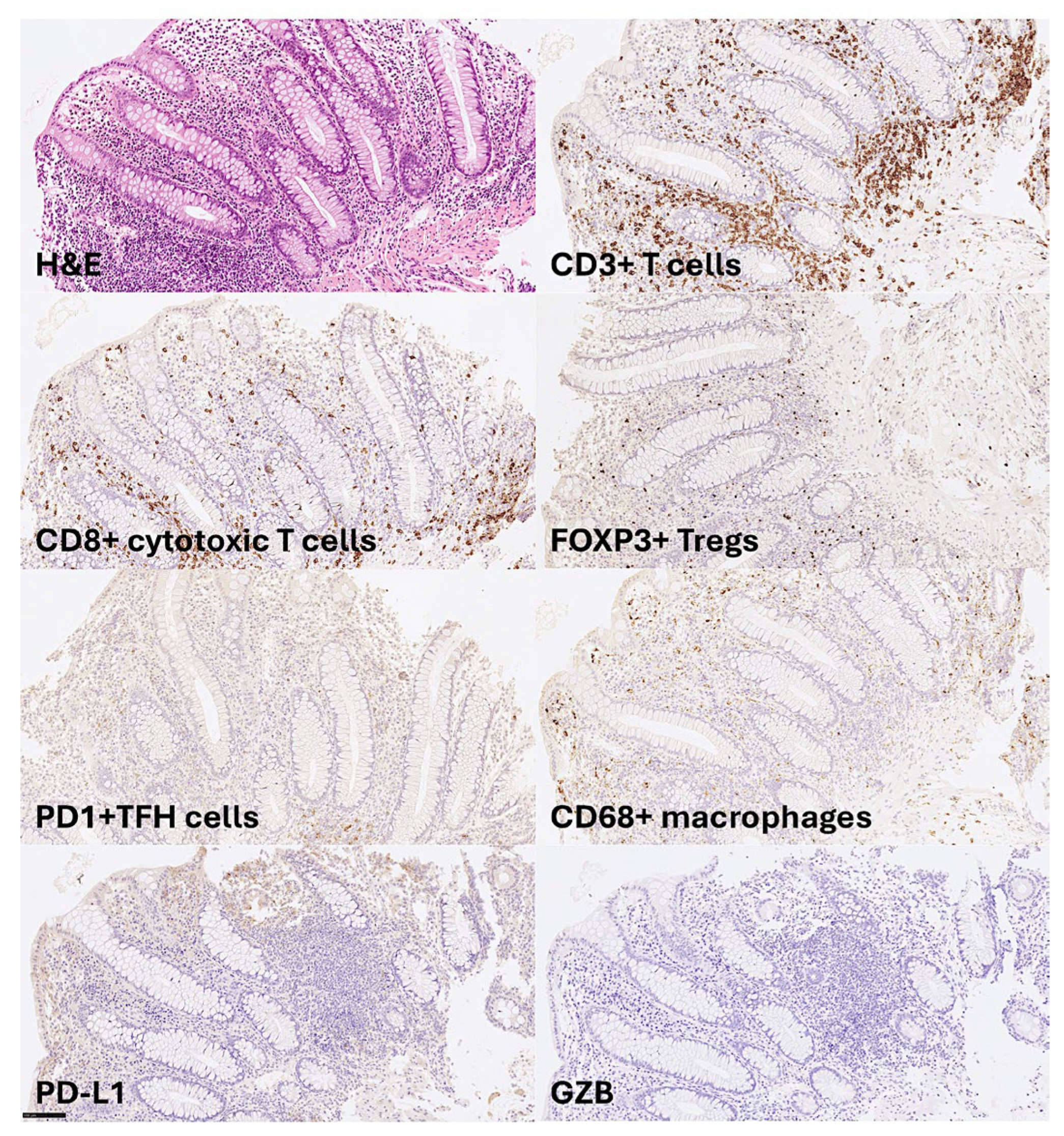
Figure 2.
Detailed visualization of some immune microenvironment components of ulcerative colitis. This figure shows the details of the tissue distribution of some of the immune microenvironment cells in ulcerative colitis at higher magnification. The lamina propria is characterized variable infiltration of CD3+T lymphocytes and CD68+macrophages. Within the CD3+T lymphocytes, cytotoxic CD8+T lymphocytes and FOXP3+regulatory T lymphocytes (Tregs) are easily found.
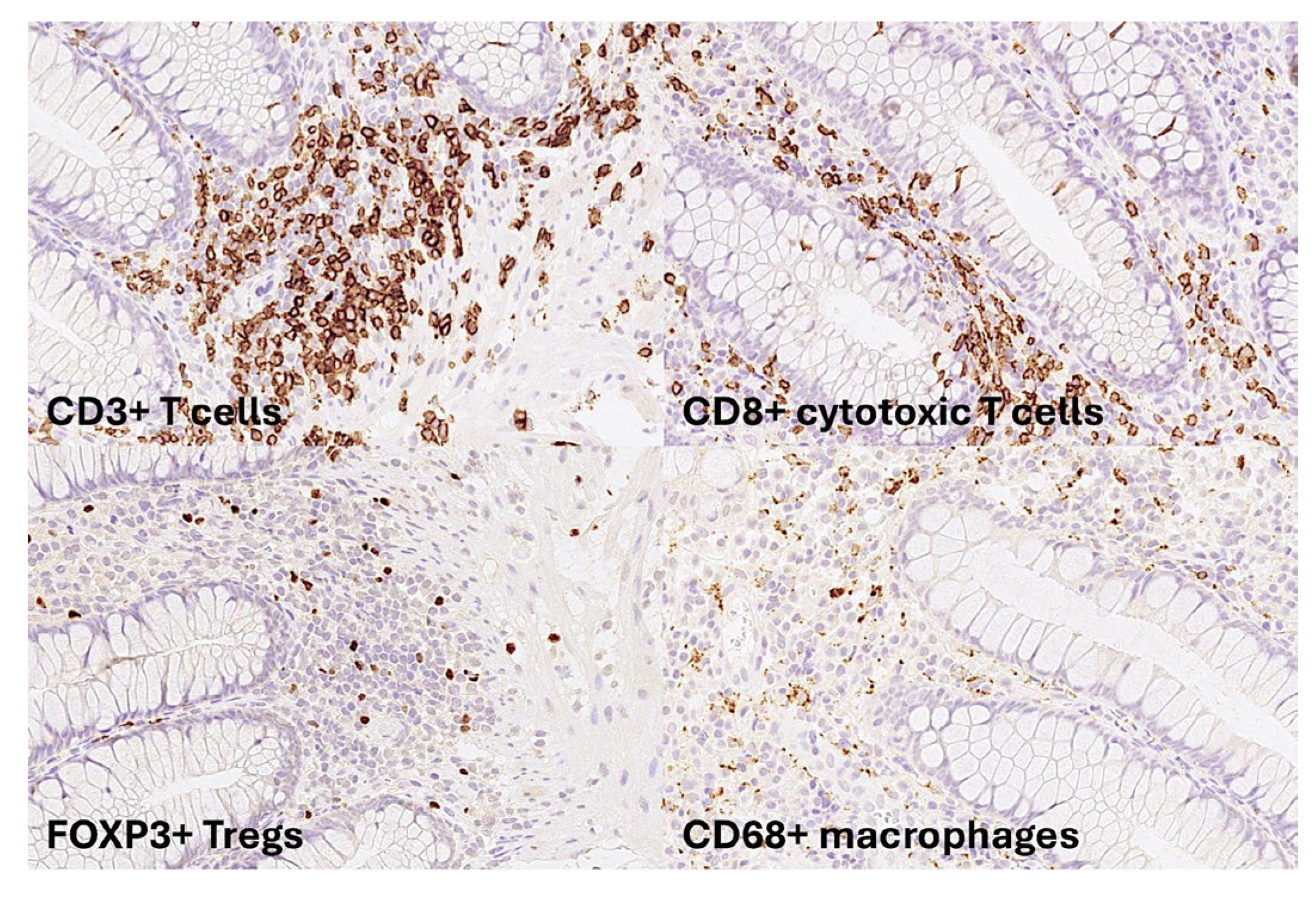
Figure 3.
Histological features of colorectal cancer. The most common histological subtype of colorectal cancer is adenocarcinoma.
Figure 3.
Histological features of colorectal cancer. The most common histological subtype of colorectal cancer is adenocarcinoma.
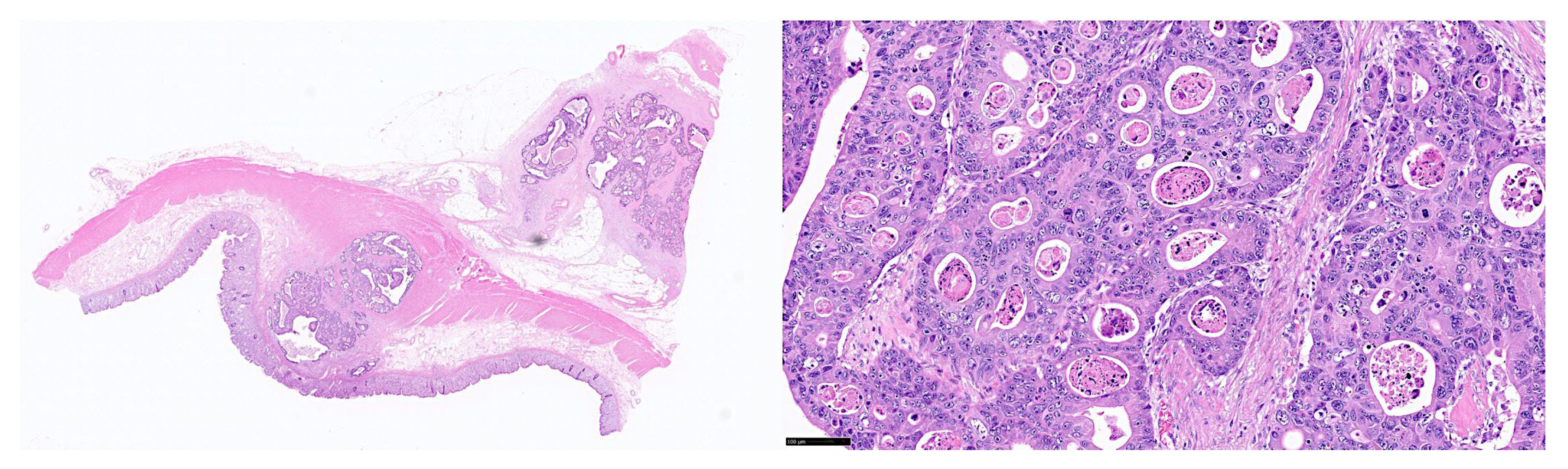
Figure 4.
Structure of a convolutional neural network (CNN). The CNN algorithm is characterized by taking an input image and assigning weights and biases to different components. Then, the deep learning algorithm performs image classification. The CNN comprises of 3 main layers: the convolutional, pooling, and fully connected layers.
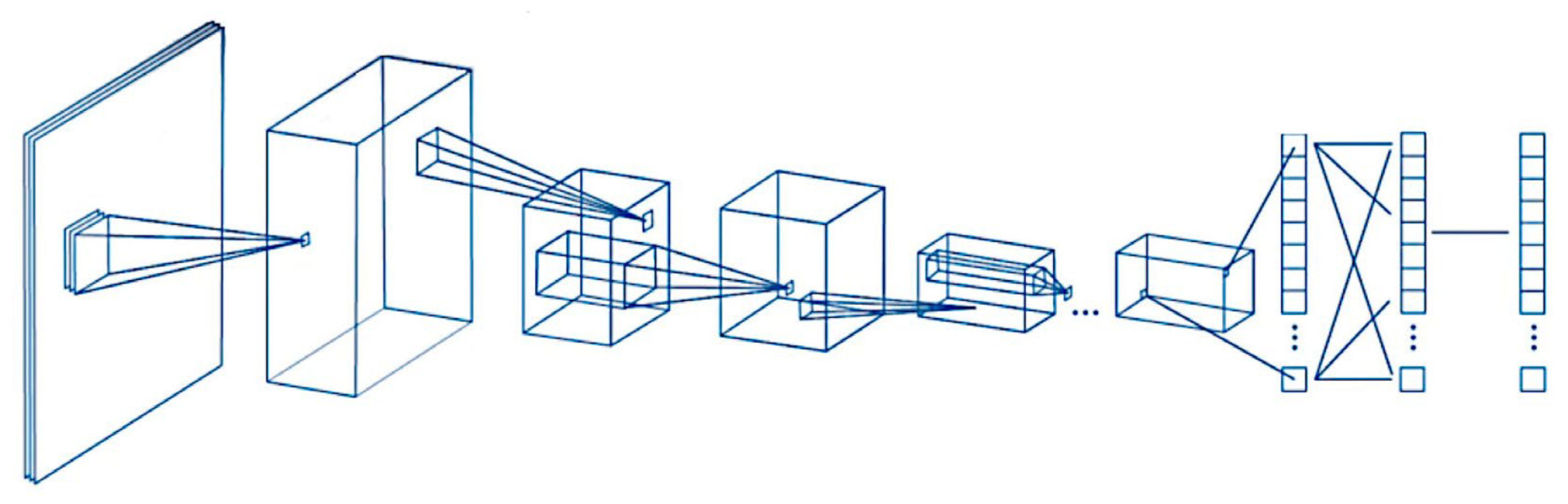
Figure 5.
Original ResNet-18 architecture.
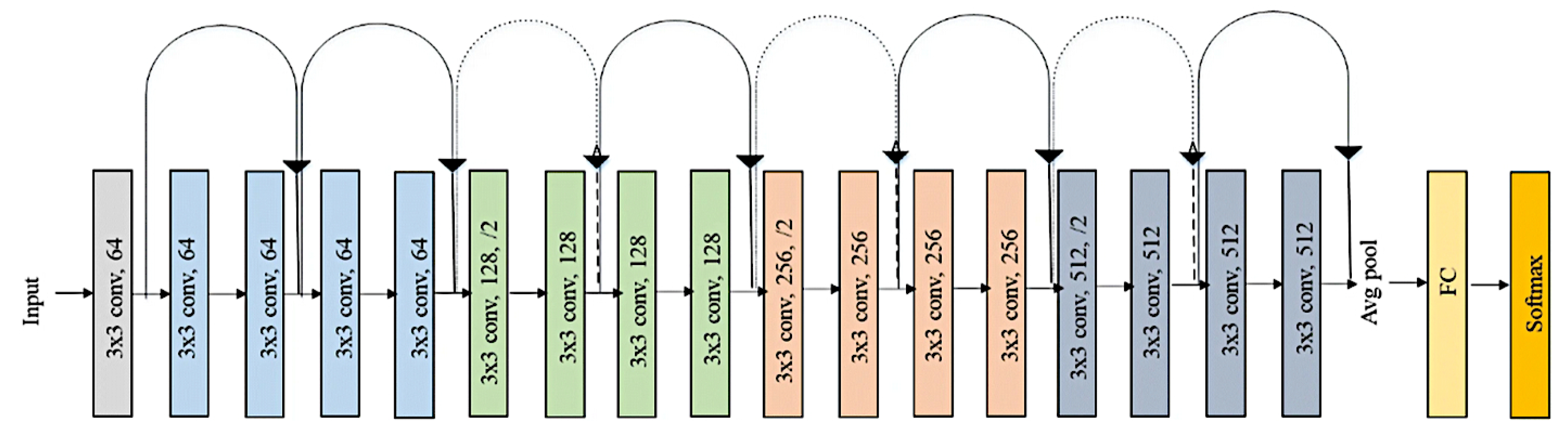
Figure 6.
Tissue processor. Processing was performed using the HistoCore Peloris 3 tissue processing system.
Figure 6.
Tissue processor. Processing was performed using the HistoCore Peloris 3 tissue processing system.

Figure 7.
Tissue embedder. The processed tissue was embedded in paraffin, forming paraffin blocs for sectioning using a tissue embedder (Tissue-Tek® TEC™ 6 Embedding Console System).
Figure 7.
Tissue embedder. The processed tissue was embedded in paraffin, forming paraffin blocs for sectioning using a tissue embedder (Tissue-Tek® TEC™ 6 Embedding Console System).
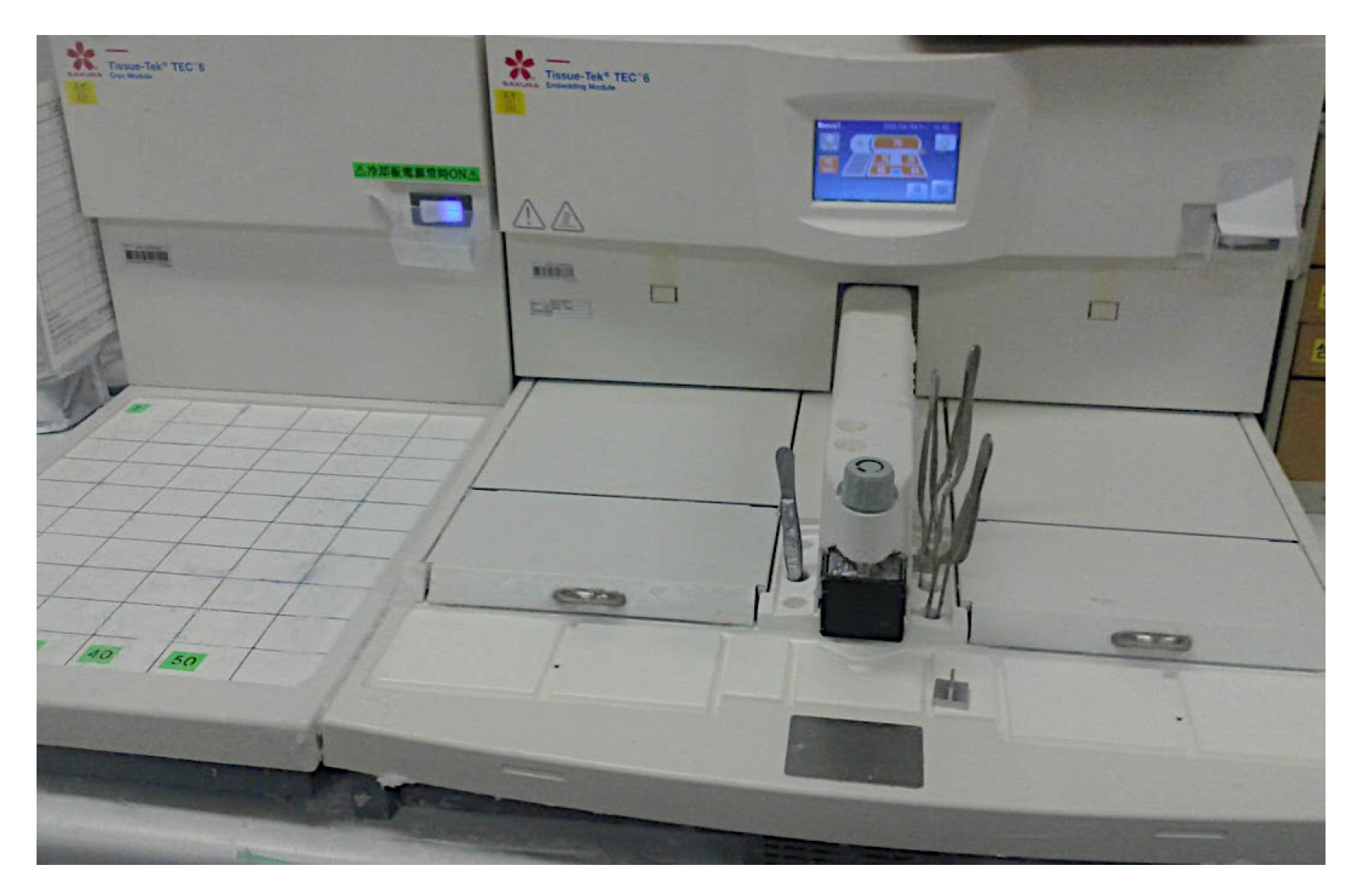
Figure 8.
Automated slide stainer. Paraffin blocks were trimmed at 2μm using a Yamato REM-710 microtome.
Figure 8.
Automated slide stainer. Paraffin blocks were trimmed at 2μm using a Yamato REM-710 microtome.
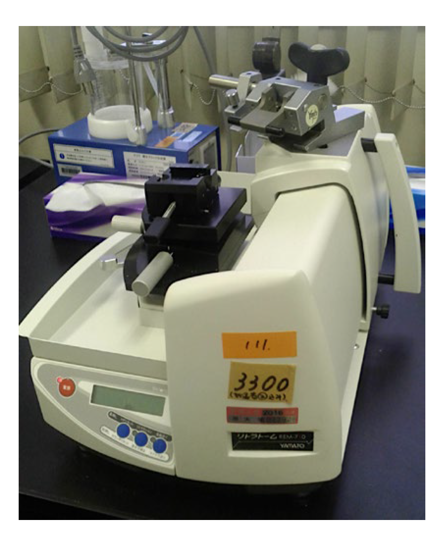
Figure 9.
Automated slide stainer. Staining was performed using a Tissue-Tek Prisma® Plus automated slide stainer.
Figure 9.
Automated slide stainer. Staining was performed using a Tissue-Tek Prisma® Plus automated slide stainer.
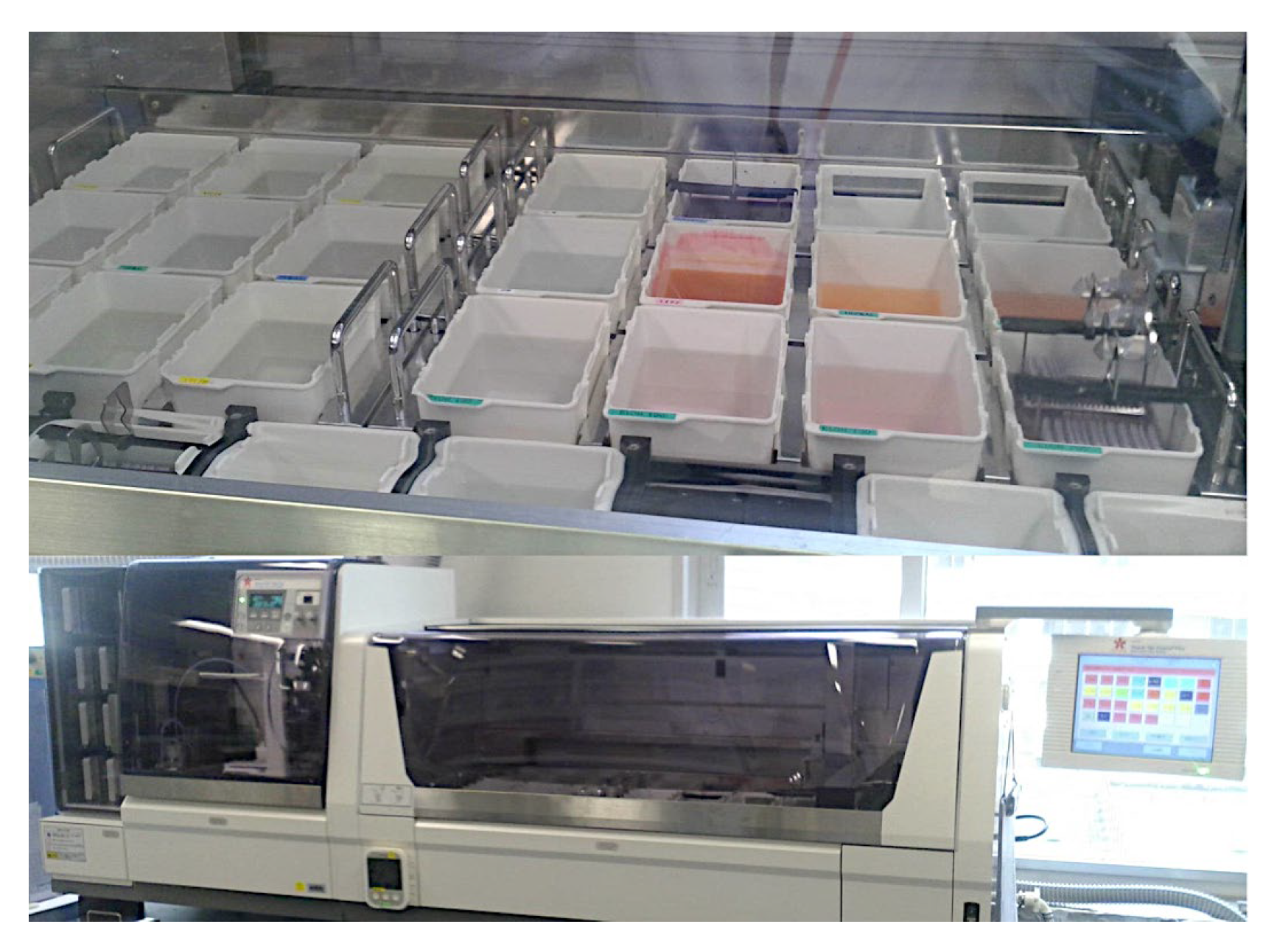
Figure 10.
Histologic Geboes score. Ulcerative colitis was assessed using the Geboes score, which ranges from grade 0 (no abnormality, left) to grade 4 (crypt destruction, right).
Figure 10.
Histologic Geboes score. Ulcerative colitis was assessed using the Geboes score, which ranges from grade 0 (no abnormality, left) to grade 4 (crypt destruction, right).
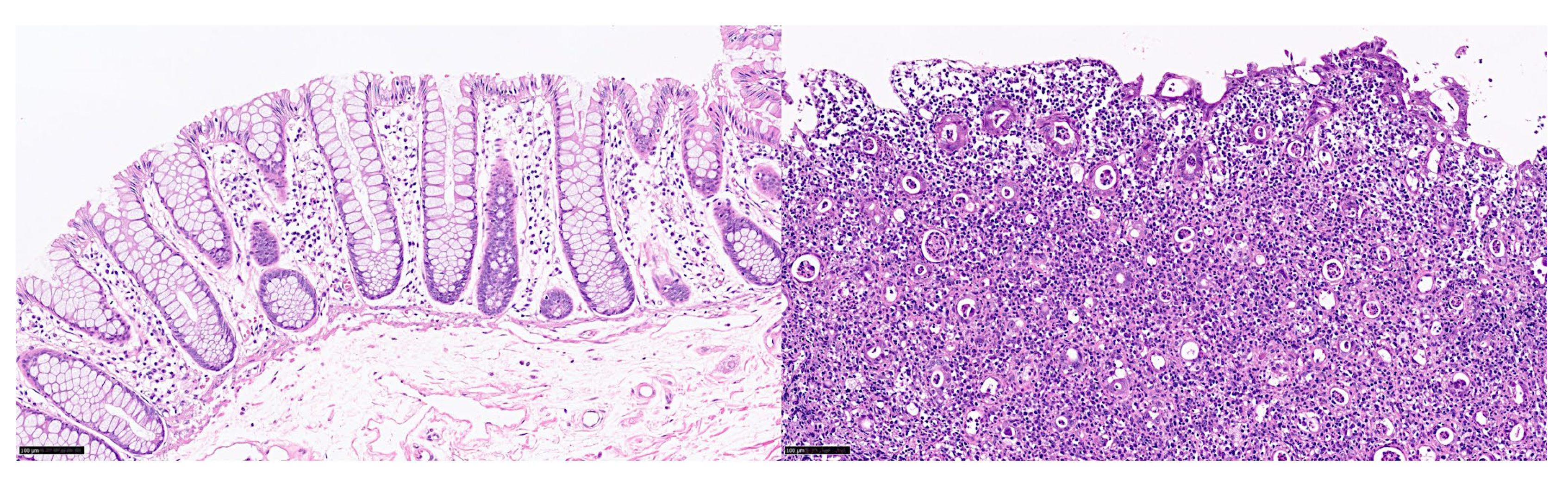
Figure 11.
Automated immunohistochemistry staining system. The immunohistochemical staining were performed using a fully automated immunohistochemistry and in situ hybridization staining system following the manufacturer’s instructions (Leica BOND-MAX).
Figure 11.
Automated immunohistochemistry staining system. The immunohistochemical staining were performed using a fully automated immunohistochemistry and in situ hybridization staining system following the manufacturer’s instructions (Leica BOND-MAX).
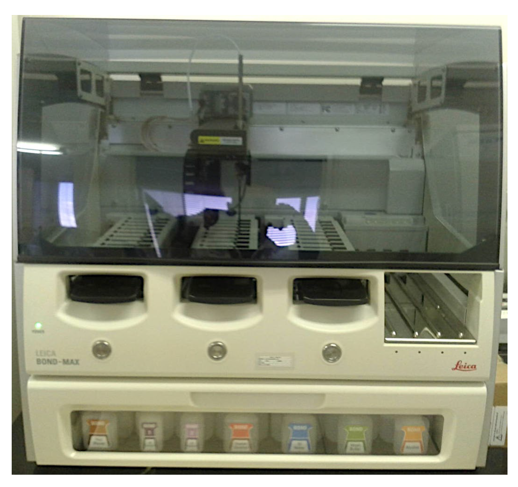
Figure 12.
Glass coverslipper for immunohistochemical tissue slides. Coverslipping was achieved using a Leica CV5030 fully automated glass coverslipper.
Figure 12.
Glass coverslipper for immunohistochemical tissue slides. Coverslipping was achieved using a Leica CV5030 fully automated glass coverslipper.
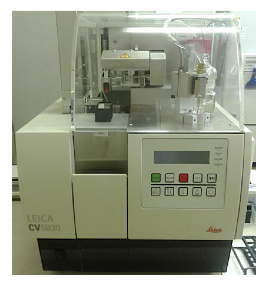
Figure 13.
Immunohistochemistry of TOX2 and LAIR1 in reactive tonsil control. TOX2 (left column) is compatible with the staining pattern of PD-1 and in the germinal centers identified follicular T helper cells. LAIR1 is a co-inhibitory receptor found on peripheral mononuclear cells, including natural killer cells, T, and B lymphocytes. LAIR1 had a pattern compatible with macrophages/dendritic cells in the germinal centers and the interfollicular areas. Additionally, the mantle zones that include naïve B lymphocytes, were positive for LAIR1.
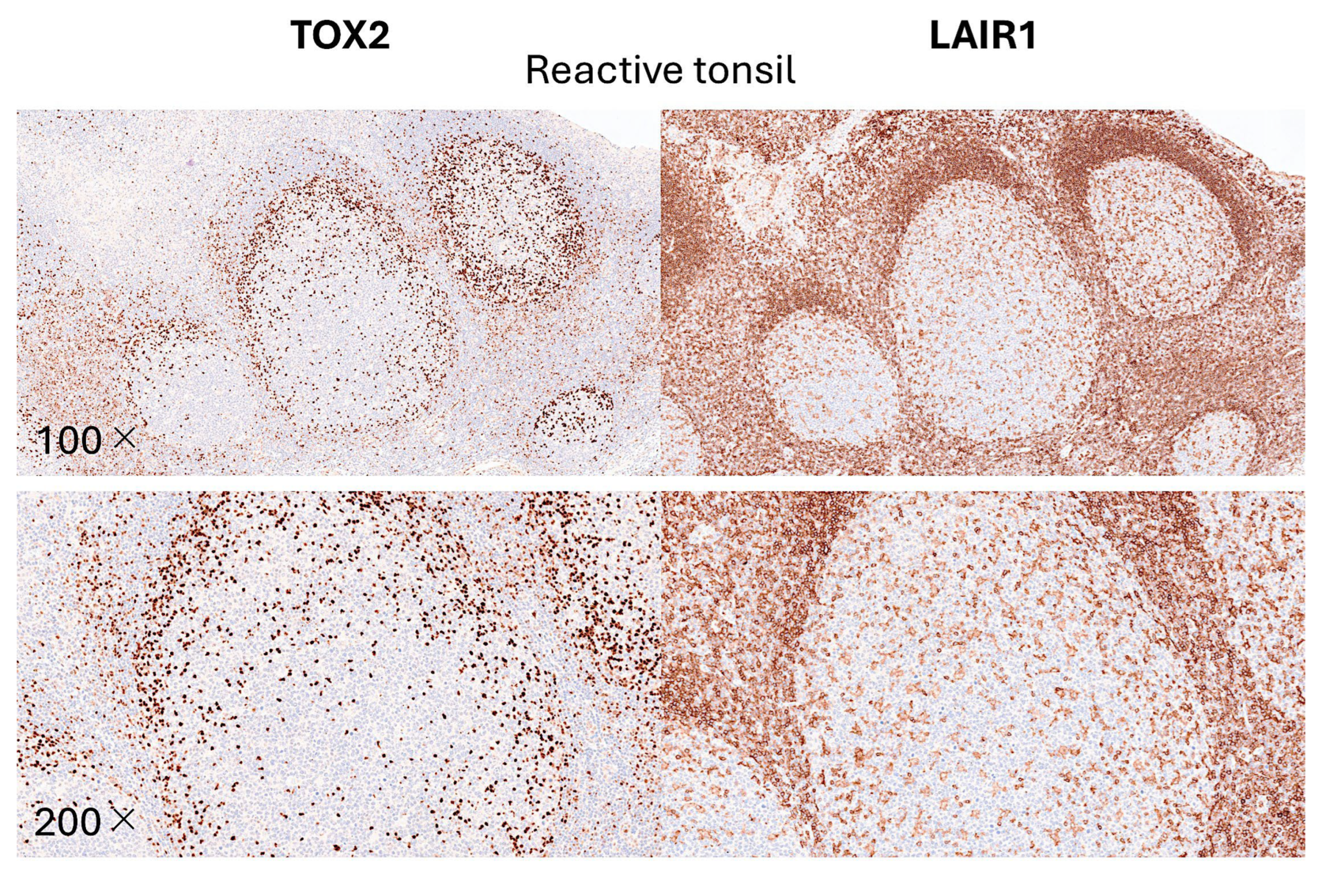
Figure 14.
Immunohistochemistry of TOX2 and LAIR1 in colonic mucosa control. TOX2 (left column) is compatible with the staining pattern of PD-1. TOX2-positive cells were also identified in the lamina propria of the mucosa. LAIR1 (right column) is a co-inhibitory receptor found on peripheral mononuclear cells, including natural killer cells, T lymphocytes, and B lymphocytes. LAIR1 had a pattern compatible with macrophages/dendritic cells.

Figure 15.
Immunohistochemistry of TOX2 in ulcerative colitis. This figure shows the TOX2 staining in the mucosa of 4 biopsies. The cases had high infiltration of TOX2-positive cells in the lamina propria.
Figure 15.
Immunohistochemistry of TOX2 in ulcerative colitis. This figure shows the TOX2 staining in the mucosa of 4 biopsies. The cases had high infiltration of TOX2-positive cells in the lamina propria.
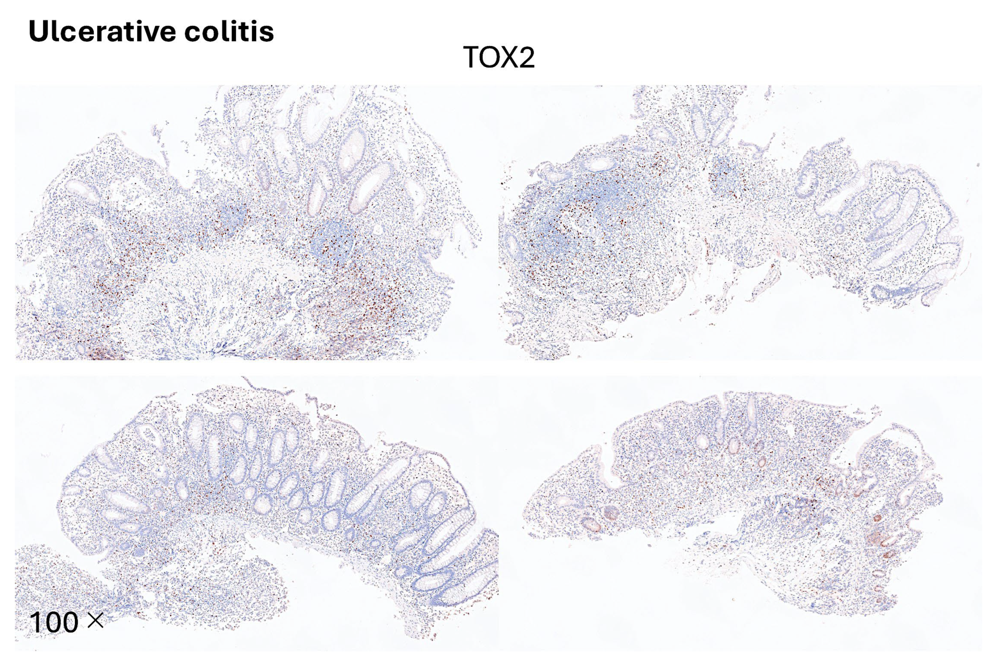
Figure 16.
Immunohistochemistry of LAIR1 in ulcerative colitis. This figure shows LAIR1 staining in the mucosa of 4 biopsies. The patients had a high infiltration of LAIR1-positive cells in the lamina propria.
Figure 16.
Immunohistochemistry of LAIR1 in ulcerative colitis. This figure shows LAIR1 staining in the mucosa of 4 biopsies. The patients had a high infiltration of LAIR1-positive cells in the lamina propria.
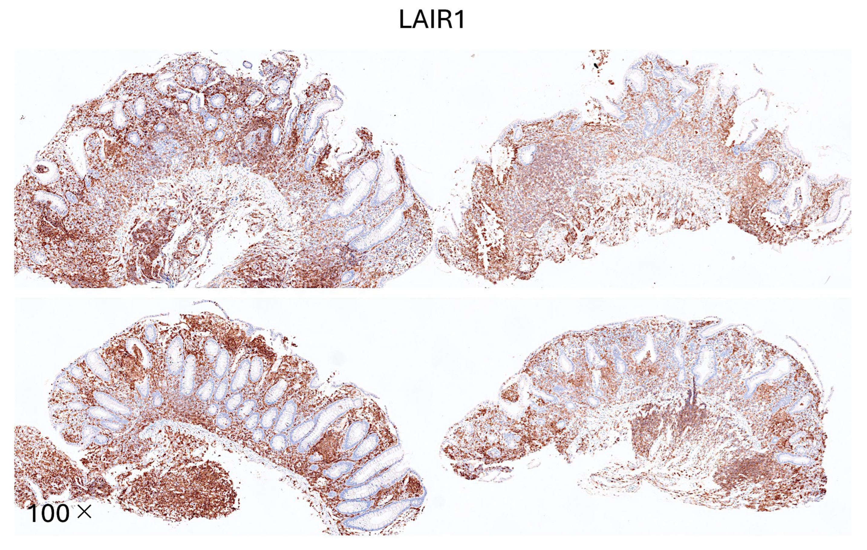
Figure 17.
Olympus upright microscope. The hematoxylin and eosin (H&E) and immunohistochemical slides were evaluated using a conventional upright microscope (Olympus BX63).
Figure 17.
Olympus upright microscope. The hematoxylin and eosin (H&E) and immunohistochemical slides were evaluated using a conventional upright microscope (Olympus BX63).
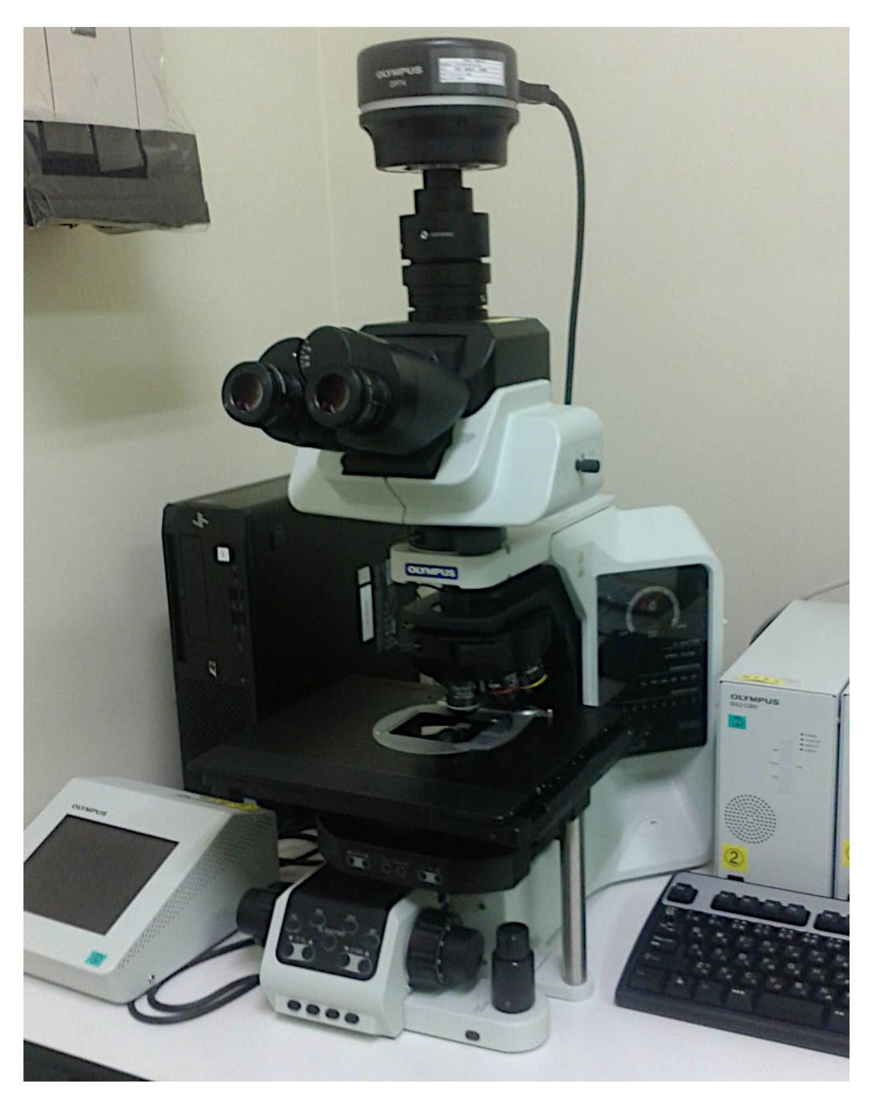
Figure 18.
Whole-slide imaging. The Hamamatsu NanoZoomer S360 scanner was used to digitalize the hematoxylin and eosin (H&E) tissue samples.
Figure 18.
Whole-slide imaging. The Hamamatsu NanoZoomer S360 scanner was used to digitalize the hematoxylin and eosin (H&E) tissue samples.
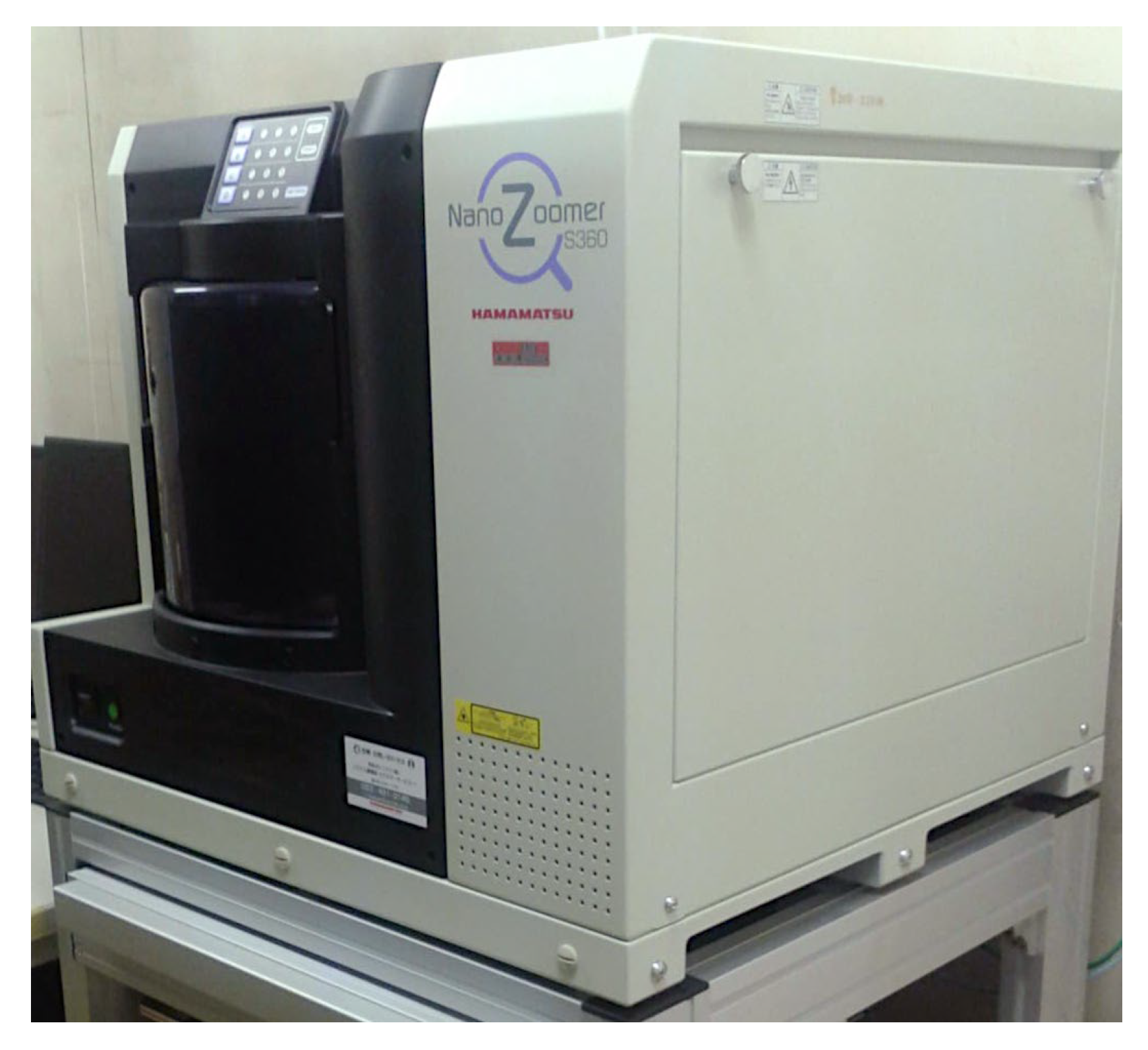
Figure 19.
Whole-slide imaging. The glass slides were converted to digital data using a Hamamatsu NanoZoomer S360 scanner that scanned the slides at 400× magnification. .
Figure 19.
Whole-slide imaging. The glass slides were converted to digital data using a Hamamatsu NanoZoomer S360 scanner that scanned the slides at 400× magnification. .
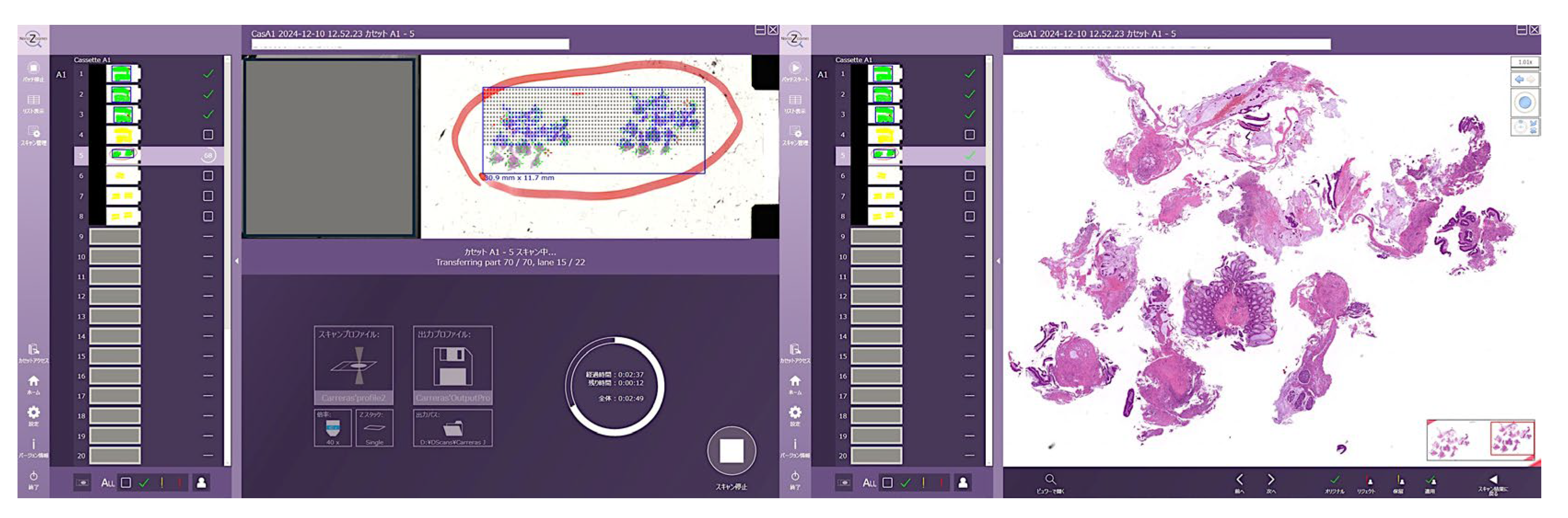
Figure 20.
Digital image quantification. Digital image quantification was performed using Fiji software. The Blue stack was used to identify the positive staining of DAB (brown) and negative pixels.
Figure 20.
Digital image quantification. Digital image quantification was performed using Fiji software. The Blue stack was used to identify the positive staining of DAB (brown) and negative pixels.
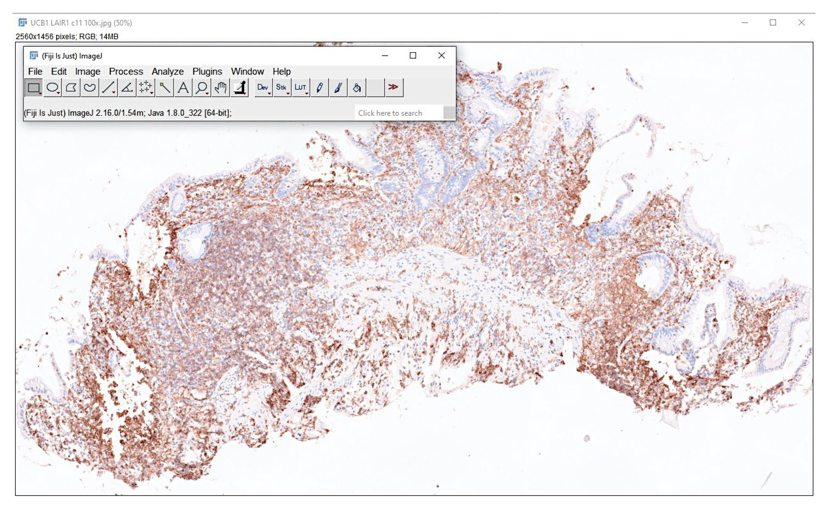
Figure 21.
Identification of regions of interest. This figure shows the hematoxylin and eosin (H&E) staining of 4 cases of endoscopic biopsy of ulcerative colitis. The areas of interest for AI analysis are indicated in yellow.
Figure 21.
Identification of regions of interest. This figure shows the hematoxylin and eosin (H&E) staining of 4 cases of endoscopic biopsy of ulcerative colitis. The areas of interest for AI analysis are indicated in yellow.
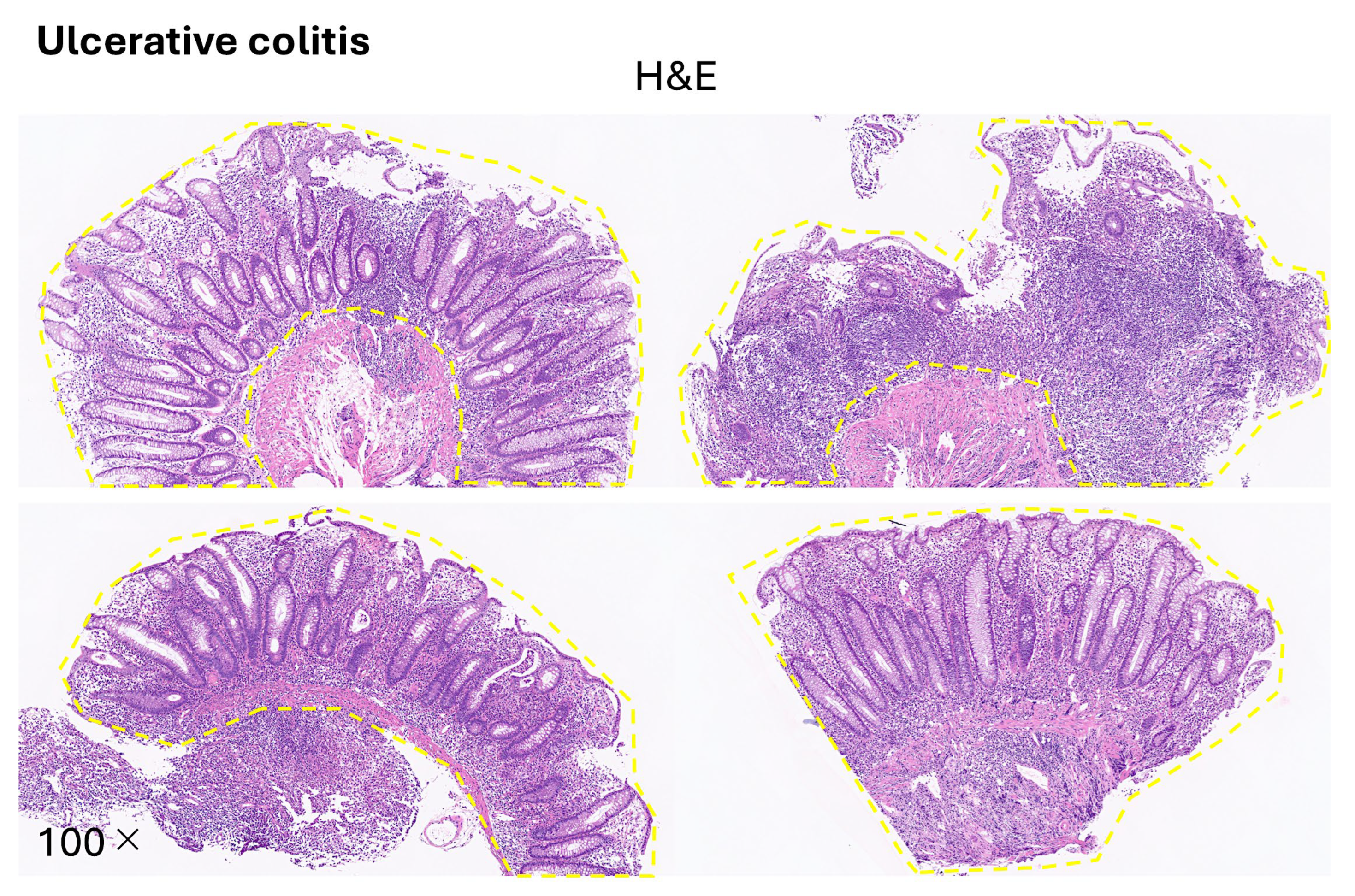
Figure 22.
Image patches of ulcerative colitis, colorectal cancer (adenocarcinoma), and colon control.
Figure 22.
Image patches of ulcerative colitis, colorectal cancer (adenocarcinoma), and colon control.
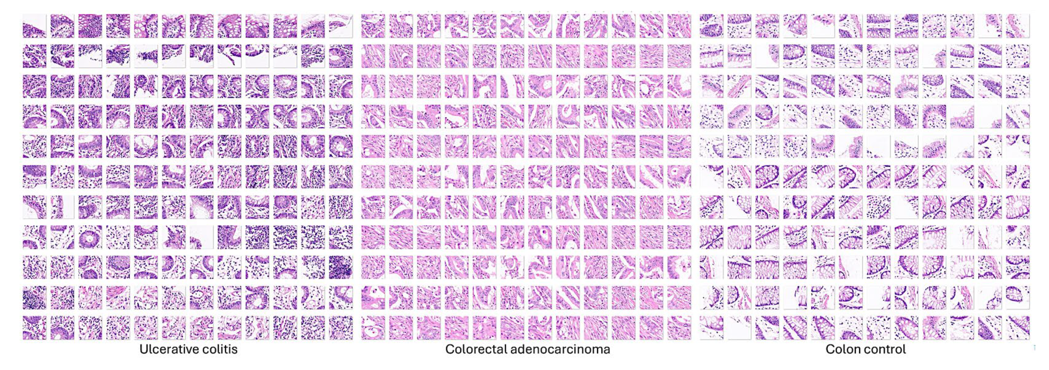
Figure 23.
Trained network layers. The CNN was designed using a transfer learning strategy and ResNet-18.
Figure 23.
Trained network layers. The CNN was designed using a transfer learning strategy and ResNet-18.
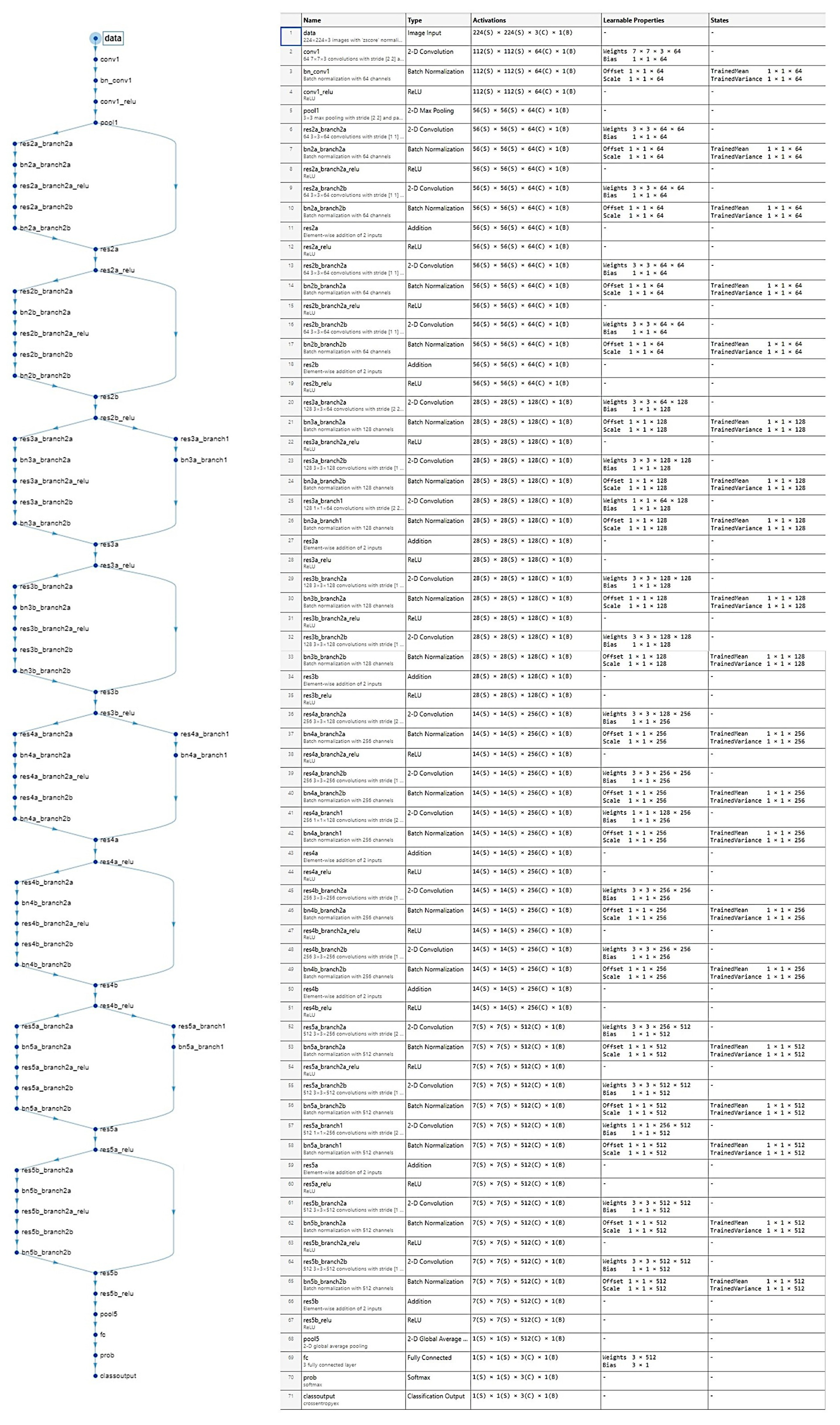
Figure 24.
Computational requirements. The desktop workstation was equipped with a Nvidia GeForce RTX 4090 graphics card.
Figure 24.
Computational requirements. The desktop workstation was equipped with a Nvidia GeForce RTX 4090 graphics card.
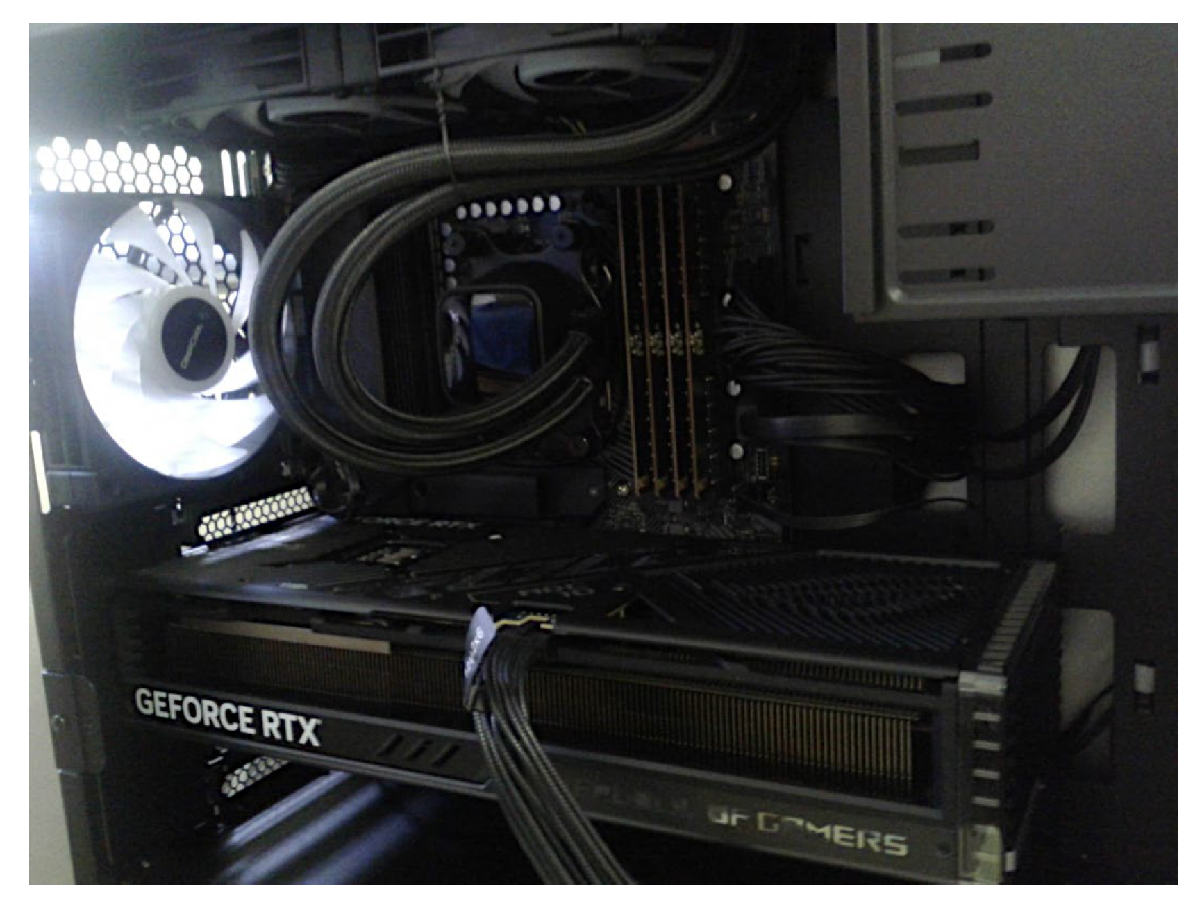
Table 3.
Design and training parameters.
| ResNet-18-Based CNN | Training (70%) | Validation (10%) | Training Options |
|---|---|---|---|
| Input type: image patches Output type: classification Number of layers: 71 Number of connections: 78 |
Observations: 59,677 Classes: 3 Ulcerative colitis: 6497 Colorectal cancer: 44,608 Colon control: 8572 |
Observations: 8525 Classes: 3 Ulcerative colitis: 928 Colorectal cancer: 6372 Colon control: 1225 |
Solver: sgdm Initial learning rate: 0.001 MiniBatch size: 128 MaxEpochs: 5 Validation frequency: 50 Iterations: 2330 Iterations per epoch: 466 |
Table 4.
Additional training parameters.
| Additional detailed training options |
|---|
|
Import images Augmentation options: none Available parameters Random reflection axis: x, y Random rotation (degrees): min, max Random rescaling: min, max Random horizontal translation (pixels): min, max Random vertical translation (pixels): min, max Resize during training to match network input size: yes, no |
|
Solver Momentum: 0.9 |
|
Learn rate LearnRateSchedule: none LearnRateDropFactor: 0.1 LearnRateDropPeriod: 10 |
|
Normalization and Regularization L2Regularization: 0.0001 ResetInputNormalization: yes BatchNormalizationStatistics: population |
|
Mini-Batch Shuffle: every-epoch |
|
Validation and Output ValidationPatience: Inf OutputNetwork: last-iteration |
|
Gradient Clipping GradientThresholdMethod: I2norm GradientThreshold: Inf |
|
Hardware ExecutionThreshold: auto. |
|
Checkpoint CheckpointPath: n/a CheckpointFrequency: 1 CheckpointFrequencyUnit: epoch |
Based on ResNet-18 transfer learning. Convolutional neural network, CNN.
Disclaimer/Publisher’s Note: The statements, opinions and data contained in all publications are solely those of the individual author(s) and contributor(s) and not of MDPI and/or the editor(s). MDPI and/or the editor(s) disclaim responsibility for any injury to people or property resulting from any ideas, methods, instructions or products referred to in the content. |
© 2025 by the authors. Licensee MDPI, Basel, Switzerland. This article is an open access article distributed under the terms and conditions of the Creative Commons Attribution (CC BY) license (http://creativecommons.org/licenses/by/4.0/).
Copyright: This open access article is published under a Creative Commons CC BY 4.0 license, which permit the free download, distribution, and reuse, provided that the author and preprint are cited in any reuse.


