
Submitted:
08 October 2024
Posted:
09 October 2024
You are already at the latest version
Abstract
Given the complexity and variability of gastrointestinal polyps, there is a growing need for more accurate machine-learning algorithms that can assist medical professionals in decision-making processes. In our study, we employed machine learning (ML) techniques to classify gastrointestinal polyps seen in colonoscopy images, that present a risk of colon cancer, affecting a large portion of the population. The dataset used in the research comprised 152 instances and included three types of lesions, totaling 76 polyps. The study consisted of applying Logistic Regression (LR) to classify gastrointestinal images. The principal motivation for choosing this algorithm consists in the fact that is preferred by many medical researchers. Another motivation consisted in the fact to compare the polyps classification accuracy of physicians and LR with optimized hyperparameters. The approached model performance was evaluated with the following metrics: Accuracy, Precision, Recall, F1_Score and Macro-average. We used the Multiclass Logistic Regression (mLR) classifier to classify polyps into hyperplastic (27.63%), serrated (19.74%), and adenoma lesions (52.63%). It should be noted that serrated polyps are hard to diagnose, even by physicians, because they have characteristics of both hyperplastic and adenoma ones. One of the objectives consisted in the study of the hyperparameters tunning of the Logistic Regression to find the best-fitted model. To check the influence of the data mix on the results obtained, for the two best models (LR with liblinear solver, L1 penalty and C = 0.01), it was performed a comprehensive statistical analysis. Based on an algorithm that admits obtaining accurate results. Such analyses are mistakenly applied in the scientific literature. The model with optimized hyperparameters achieved an accuracy score of 70.39%, indicating a reasonable level of prediction, surpassing both beginner and expert physicians and obtaining results similar to those obtained by Random Subspace and Random Forest. The model successfully classifies the hyperplastic and adenoma polyps but showed to have a more limited ability to predict the serrated ones.
Keywords:
Medical Imaging
; Gastrointestinal Polyps
; Machine Learning
; Smart Techniques in Healthcare
; Classification problem
; Logistic Regression algorithm
; Multinomial classifier
; Colorectal disease
; Clinical Decision Support System
; Medical Diagnosis
1. Introduction
The statistic that cancer claimed approximately 9.6 million lives in 2018 [1,2] refers to worldwide data. This number represents the global impact of cancer across 185 countries, not the statistics for any specific country. Among the myriad forms of cancer, lung, bone, and colorectal cancers dominate the global landscape, with colorectal cancer standing out as one of the most prevalent malignancies, particularly affecting the elderly. Fortunately, the incidence of colorectal cancer in certain adult and elderly populations has been declining, attributed in part to regular screenings such as colonoscopies [3], which have been shown to reduce mortality rates in case it is identified in the early stage.
Colorectal cancer reaches both colon and rectal cancer, with adenocarcinoma being the most frequently encountered subtype, accounting for over 90% of all cases. Regardless of the effectiveness of colonoscopy as the primary screening method for colon cancer, its imperfections are evident, with a notable rate of undetected precancerous lesions and atypical cancers, indicating a need for further clarification [4,5,6].
Historically, colonoscopy has been the gold standard for detecting and diagnosing colorectal polyps. Colonoscopy involves a series of steps, starting with bowel preparation wherein patients consume a specific solution to cleanse the bowel, ensuring optimal conditions for the procedure. Subsequently, a colonoscopy equipped with light and a camera is inserted into the rectum for examination [7,8].
From a machine learning (ML) standpoint, colorectal polyp detection is a complex problem that requires training a model to recognize features indicative of a polyp from images or live video streams. These models are often fine-tuned and augmented to enhance performance and classify different polyp types [9].
Colorectal polyp detection models typically aim for one of three objectives: polyp segmentation [10,11], detection [12,13], or classification [14]. Some models are trained to fulfill multiple objectives concurrently, such as detecting or segmenting polyps followed by classification [15]. Detection models learn to localize polyps in images by processing training images alongside their labels, which typically include bounding box coordinates and polyp presence indicators. Segmentation models, on the other hand, are trained to outline polyps in colonoscopy images using corresponding image masks as labels [16]. Lastly, classification methods identify polyps without determining their location.
Feature extraction is a fundamental aspect of image analysis, especially in the field of medical imaging [17], where accurate diagnosis and treatment depend to a high degree on the interpretation of visual data. Gastroenterological studies, in particular, necessitate complex feature extraction techniques due to the complex nature of gastrointestinal pathologies [18].
Classification of complex lesions in real-time [5,19] presents a challenge due to slight distinctions between benign and malignant lesions. Colonoscopies currently utilize two main imaging techniques: Narrow Band Imaging (NBI) and conventional White-Light (WL) high-resolution endoscopy [20,21]. NBI, employing green and blue wavelengths, enhances visualization by highlighting blood vessels, aiding in lesion characterization. Conversely, WL endoscopy evaluates polyps based on their appearance under white light, sequentially predicting histology.
During colonoscopies, clinicians capture images of tumor masses known as polyps, which necessitate accurate classification as either benign or malignant to guide appropriate treatment decisions. Various classification systems with some limitations such as Kudo [22], Sano [23], and Paris [24] are employed for this purpose. In addition to facilitating accurate clinical decision-making, minimizing procedure duration and costs, and reducing the need for subsequent investigations are notable advantages.
Tian et al. [13] explore the use of a Deep Neural Network for detecting, localizing, and classifying polyps in videos obtained during colonoscopies. The proposed model utilizes a flexible endoscope to capture video images of the colon, which are then automatically analyzed to identify potential anomalies, such as polyps, which are precursors to colorectal cancer. The model is based on an advanced Convolutional Neural Network (CNN) architecture and includes a two-stage method for detecting and classifying polyps, using the Softmax function to determine whether a region in the image belongs to a polyp or non-polyp category. The model’s performance is evaluated using metrics like ROC-AUC, which helps assess its ability to distinguish between classes.
In the paper [25], Qinwen et al. focus on the creation and assessment of various ML models to predict colorectal polyps based on electronic health records. The study concludes that ML models, particularly AdaBoost, offer a non-invasive and cost-effective strategy for predicting colorectal polyps, potentially guiding screening and treatment decisions.
In previous research [26], we applied four other ML algorithms (Support Vector Machine, Random Forest, Random Subspaces and Extra Trees), of which Random Forest performed best.
Multiclass Logistic Regression (mLR) is frequently used by medical researchers based on this fact its study is very important. Model fit is an important subject that must be studied in rigorous research based on ML, which is the case of mLR hyperparameters tuning a difficult task. In this research, we studied the state-of-the-art mLR algorithm to determine the best-fitted hyperparameter tuning for the problem of gastrointestinal polyp image classification in adenomas, serrated and hyperplastic which is difficult even for physicians. It must be noticed that serrated are difficult to define, since they exhibit features of both hyperplastic and adenoma; based on this fact are difficult to identify accurately even by expert physicians [27]. Serrated lesions can cause 8-15% of all colorectal malignancies. Specifically, we focus on comparing mLR with other important algorithms, used by Mesejo et al. [14], as well as comparing against two categories of physicians beginners and experienced. The experimental results for both ML algorithms and human clinicians were sourced from [14].
The subsequent sections of the paper are structured as follows. Section 2 presents the dataset, binary mLR and performance metrics used in this work, conducted in the Gastrointestinal Polyps classification from colonoscopy images and briefly outlines the proposed methodology employed in this study. In Section 3, the results obtained from experimental investigations are presented, and our results are compared to other methods and the results of physicians with different levels of experience. Section 4 presents the conclusions and future work.
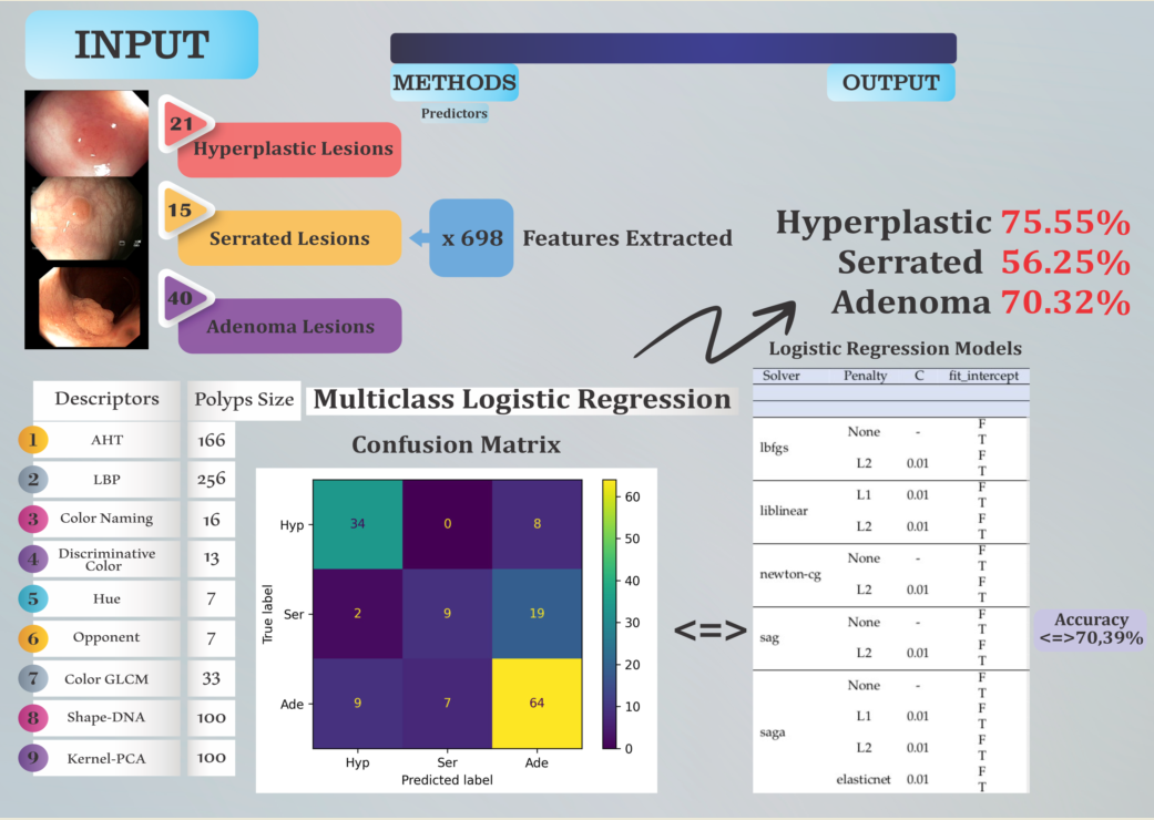
Figure 1.
An overview on the research performed on classification of gastrointestinal polyps. Note that the best logit models are obtained when a few instances of the serrated class are extracted in the test set. The higher the number of images extracted and serrated in the test set, the lower the accuracy of the algorithms.
2. Materials and Methods
2.1. Colonoscopy Dataset
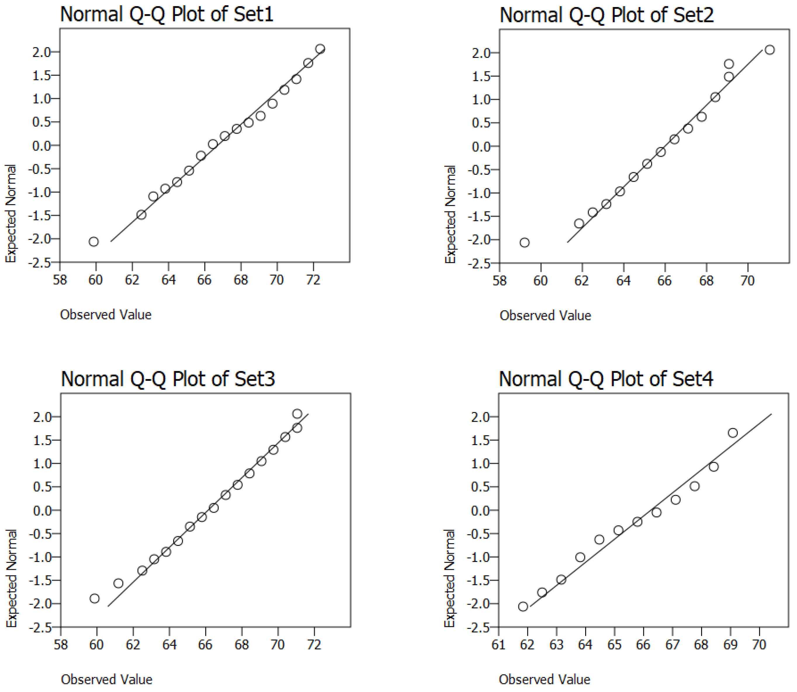
The trustful accurate colonoscopy dataset is a complex video and picture dataset of 76 polyps, that was introduced in [14]. The dataset consists of 152 brief colonoscopy videos, 152 photos (768 × 576 pixels) and 698 features extracted from every photo available at
The polyps in this dataset are divided into three categories: 21 hyperplastic, 40 adenoma, and 15 serrated lesions. As part of their everyday protocol, the doctors captured two pictures during colonoscopies using WL and NBI, respectively for every polyp, they obtained one WL image and one NBI image.
After transposing the file, it contains the following information:
- 1st column: name of the lesion;
- 2nd column: class of lesion (hyperplastic - 1; serrated - 2; adenoma - 3);
- 3rd column: type of light used (one row with White Light (WL) and the other with Narrow Band Imaging (NBI), resulting in 152 rows instead of just 76);
- 4th column until the last one (701): features.
The three different forms of lesions — adenoma, hyperplastic, and serrated — are shown in Figure 2, going from left to right. Mesejo et al. [14] present gastroenterologist opinion, with two knowledge levels: 3 beginner and 4 expert physicians, as well as the ground truth (i.e., histological classification).
The beginner and expert opinions are only based on endoscopic image data without knowing any other clinical information, meaning that the medical doctors were tested similarly with the same data as the ML algorithms.
Even though hyperplastic and tubular adenomas, which are benign, are the most prevalent polyps detected in patients, their potential to develop malignancy if left undetected and untreated over an extended period is major [12].
2.2. Feature Extraction
For every image, a rich dataset of 698 features including 2D texture, 2D color, and 3D shape descriptors are obtained, providing a gastroenterological image characterization.
2D Texture Features: Gastroenterological images frequently have complicated textural differences that provide key diagnostic information. Invariant Gabor Texture Descriptors (AHT) [28] and Invariant Local Binary Patterns (ILBP) [15] can capture accurate texture differences. AHT, based on Gabor filters, improves in storing texture information uncompromised by illumination, rotation, or scaling changes. In contrast, ILBP gives binary representations of texture patterns, allowing texture analysis in a shorter time.
2D Color Features: Color information in gastroenterological images can provide a helpful understanding of tissue features and anomalies. Hue and Opponent histograms [29], coupled with Color Grey-Level Co-occurrence Matrix (Color GLCM), Discriminative Color [30] and Color Naming [31], create a full collection of color characteristics. These descriptors accurately capture color variations, semantic color distributions, and discriminative color features, allowing for an exact definition of gastrointestinal lesions and tissues.
3D Shape Features: The three-dimensional shape of gastrointestinal polyps has important diagnostic implications. 3D reconstruction utilizing Structure from Motion (SfM) [32] approaches enables faster retrieval from data. Shape DNA [33] and Kernel PCA [34] are effective techniques for representing polyp surface signatures and spatial architecture. These descriptors allow the characterization of non-rigid structures while also making use of the confusing spatial connections found in gastroenterological images. The first row contains the video name and the second row is the ground truth, the real diagnosis of hyperplastic, Serrated and Adenoma, does not depend on the doctor’s assumptions based on images. The features extracted are the following [14]:
- Amplitude Histogram of Texture (AHT) - 166 features. This texture descriptor captures information about the distribution of amplitudes in images.
- Local Binary Patterns (LBP) - 256 features. This texture descriptor measures the local distribution of binary patterns in an image.
- Color Naming - 16 features. These represent descriptions of colors in images, classified into a predefined set of color names.
- Discriminative Color - 13 features. This descriptor captures information about dominant and discriminative colors in images.
- Hue - 7 features. These are characteristics describing the predominant color hues in the image.
- Opponent - 7 features. This descriptor refers to the representation of colors in an opponent color space.
- Color Gray-Level Co-occurrence Matrix (GLCM) - 33 features. This is a descriptor that analyzes the distribution of textures and contrasts in images.
- Surface Signatures with Shape-DNA - 100 features. This descriptor refers to the representation of object shapes in images using a DNA-based model.
- 3D Cloud Signatures with Kernel-Principal Component Analysis (PCA) - 100 features. This is a descriptor that performs a principal component analysis on a dataset in an implicitly defined feature space generated by a kernel.
- Within the output file, the first row contains the movie name associated with the image, and the second row contains the ground truth value associated with the image. This information can be useful in evaluating the performance of the models or algorithms used in the work.
- By using this output file, we have access to a detailed and multidimensional representation of the images, which can be used in various image analysis and recognition applications.
2.3. Methods
Mesejo [14] system’s input is a video recorded during explorations by clinicians. This exploratory video, lasting approximately 30 seconds to one minute, captures lesions from various perspectives, slowly orbiting around them using both Narrow Band Imaging and White Light. This video does not entail any deviation from the usual medical protocol; the clinician recorded it naturally, meaning it closely resembles their daily practice. Every second of the recording consists of 30 frames of 768 × 576 pixels [14]; therefore, any other video format could have been used.
The point about the protocol essentially refers to the fact that they filmed in their usual manner, as they do every day. Four experts and three beginners evaluated the dataset [14], meaning, as implied by the confusion matrix, that all were given the 152 images to analyze. It is important to emphasize that the difficulty of classifying colorectal lesions for human operators in our case is greater than in a real-world scenario. Later, clinicians can move freely around the lesion and know the lesion’s location in the colon. Of course, classification accuracy could be improved by introducing additional information, such as the lesion’s position, with those on the right side, while others are found in the left colon. The aim was to provide the same information to both the ML system and the human operators.
How were contradictions resolved? That’s the opinion; all were given the 152 images, and in this way, they diagnosed them, inevitably making mistakes. Here, we have the confusion matrix of the experts. It shows that they correctly identified, 14% of hyperplastic lesions, 9.5% of serrated lesions, and 25.5% of adenomas; the experts made significant errors, as you can see, and the beginners made even more. It is evident here that instead of 14, they identified only 11, 6.7, and 26; in fact, the beginners were even better than the experts, at least regarding adenomas.
We used two descriptors for texture features, five for color features, and two for 3D shape features. We characterize each polyp with a numerical fingerprint, i.e., a signature obtained from the reconstructed 3D structure. In this context, the shape signatures need to be invariant to the scaling, rotation, and translation of shapes.
We rely on Structure from Motion (SfM) method to calculate the density of the 3D model. Essentially, the polyp was reconstructed in 3D, and the reconstruction was carried out through an SfM procedure. Thus, it is not a fingerprint or descriptor; the surface signature using shape DNA is the descriptor. Thanks to dense SfM, we have a description of the polyp’s surface using a triangular mesh, which allows us to calculate the magnitude of the surface in terms of both normal and curvature. Specifically, we use shape DNA features, but similarly, based on spectral analysis, shape DNA is invariant.
We extracted 3D shapes using SfM, which takes a short video as input. However, thanks to SfM, we have a description of the 3D surface using a color mesh. This allows for surface calculation, making the 3D cloud invariant to scaling and rotation.
The principle involves constructing a tree and partitioning the predictor value space for training. In simpler regions, a set of rules is applied. The algorithm then predicts response values by considering the predictors introduced later in the observation.
The recursive method is often used to split the predictors into binary categories. The process begins at the tree’s root, where all observations belong to a single region, and a binary split is made at each step.
Logistic regression (LR) is a supervised ML algorithm, used for binary (called binomial LR) or multinomial classification (called multinomial LR).
Employing an LR function followed by a threshold function results in an LR classifier [35]. However, the binary nature of the threshold introduces challenges: the hypothesis lacks differentiability and represents a discontinuous function of inputs and weights, making learning with the perceptron rule quite unpredictable.
In logistic regression (LR), the probability of a particular outcome is modeled using the logistic function, which takes the following form [36]:
In this equation, denotes the probability that the dependent variable is equal to 1, given the value of the independent variable X. The term is the intercept, representing the predicted log-odds of the outcome when . The coefficient quantifies the effect of the independent variable X on the log-odds of the outcome. The symbol e refers to the base of the natural logarithm, ensuring that the function’s output is constrained between 0 and 1.
Through some manipulation of equation (1), we find:
The expression , known as the odds, represents the ratio of the probability of an event occurring to the probability of it not occurring. While probability ranges between 0 and 1, odds range between 0 and ∞. Odds close to 0 indicate a low probability, whereas odds approaching ∞ indicate a high probability.
Probability, , measures the likelihood of an event occurring, ranging from 0 to 1. For example, the probability of rolling a 3 on a fair six-sided die is .
Odds and probability values are nearly the same for rare (unusual) occurrences when is very small, because . For example, the odds of rolling a 3 on a fair six-sided die can be calculated as:
The left side of equation (2), or the log odds, is obtained by taking the logarithm of both sides. A linear logit is created through the LR model in X.
These challenges can largely be addressed by replacing the hard threshold function with a softened version and approximating it with a continuous, differentiable function. We explored two such functions resembling soft thresholds: the integral of the standard normal distribution (utilized in the probit model) and the logistic function (used in the logit model). With the logistic function replacing the threshold, we redefine:
Specifically, the output, ranging from 0 to 1, can be interpreted as the probability of belonging to class 1. This hypothesis delineates a soft boundary in the input space, assigning a probability of 0.5 to inputs at the boundary’s center and tending towards 0 or 1 as we move away from it.
In the case of LR, due to its non-linearity, there is no direct analytical solution for optimizing the loss function (log-likelihood). For its maximization, numerical methods are used, such as Limited-memory Broyden–Fletcher–Goldfarb–Shanno (lbfgs), Library for Large Linear Classification (liblinear), Newton Conjugate Gradient (newton-cg), Newton’s Method with Cholesky Decomposition (newton-cholesky), Stochastic Average Gradient (sag) and Stochastic Average Gradient with Acceleration (saga).
The (lbfgs) [37,38,39] solver is an analog of Newton’s Method, and the liblinear [40,41] optimizes the loss function by iterating over each coefficient of the model and adjusting it while the other coefficients are held constant. The newton-cg is a solver that uses the conjugate gradient Newton-Raphson method for optimization, while newton-cholesky solver is a variant of the Newton-Raphson method that uses the Cholesky decomposition to solve the system of equations derived from the Newton-Raphson method. The Sag [42] and saga (a variant of sag) [43] are solvers that use stochastic variants of gradient optimization and they are efficient for large and sparse datasets. Unlike the other solvers, saga supports both L1 and L2 regularization as well as their mixture (ElasticNet).
Data normalisation refers to the process of transforming the values in a set of data so that they are on a common scale, usually between 0 and 1, or have a mean of 0 and a standard deviation of 1. In general, most ML algorithms perform better when the data is normalised. Normalisation of data is important to ensure that all features contribute equally to the final result. Thus, it is prevented that certain characteristics dominate others due to their different scales [44].
Dataset preparation. Because the original dataset was ordered according to the label, we first shuffled the rows randomly and for reproducibility, we used random_state=42. Random_state is a parameter used in Scikit learn, to control randomness in various procedures. It is a way to set a seed for the random number generator, thus ensuring reproducibility of the results. In the KFold context, random_state controls the shuffling of the data before it is split into folds for training and test, respectively. When re-running experiments, using a fixed random_state ensures that data splits and results will be consistent.
2.4. Performance Metrics
To evaluate the quality of the multinomial classification model prediction, we used (1) Confusion Matrix and the following metrics: (2) Accuracy, (3) Precision, (4) Recall (called also Sensitivity), and (5) F1-Score. The confusion matrix is useful for computing important performance metrics. The Accuracy, Precision and Recall (or detection rate) for multinomial classification have been described in [26].
Confusion Matrix is a tool used in the ML field to evaluate the performance of a classification algorithm. This is a square matrix of n×n size, where n represents distinct class numbers. Every element (i, j) of the array indicates the number of instances in the class i that were classified as belonging to the class j.
In the binary classification, the matrix has four elements: TP (true positive - positive examples number correctly classified), TN (true negative - negative examples number correctly classified), FP (false positive - number of negative examples incorrectly classified as positive), and FN (false negative - number of positive examples incorrectly classified as negative) as can be seen in Table 1.
This is the confusion matrix. Here, we have the binary case of true positive, false negative, and vice versa. Generally, algorithms tend to invert negative and positive from the actual values, and here we have the predicted ones. For instance, recall, which is sensitivity, is calculated as true positives divided by the sum of the entire row. All these metrics are crucial for binary classification. Precision and recall are emphasized because, for example, selectivity is merely an inverse of sensitivity, meaning that in multinomial classification, many other metrics lose their relevance compared to binary classification.
In the case of multinomial classification problems, the confusion matrix expands to include all classes of the problem. It can be considered that each class has its terms TP, TN, FP and FN. Thus, the matrix confusion allows a detailed analysis of how the model performs corrects and misclassifications for each class. Table 2 exemplifies a confusion matrix for a problem with three classes.
where:
- , , are True for class A, class B, and class C, respectively.
- are False, that is class i is wrongly predicted as belonging to class j
F1_Score is the Harmonic mean of Precision and Recall. It is useful when there is an imbalance between the number of items of classes of the given problem, providing a unique measure of a model’s performance by combining precision and recall. F1_Score for binary problems is shown in Equation (5). For multiclass problems, F1_Score is calculated for each class (see Equation 6).
Macro_average is the arithmetic mean of Precisions, Recalls and F1-Scores. It is a method of aggregating the performances of classification models, instrumental in multiclass classification problems. Like F1_Score, it is helpful in unbalanced datasets where some classes are under-represented because it gives equal weight to each class. This avoids situations where the model’s performance on large classes dominates the overall evaluation and provides better clarity on the model’s performance for all classes.
The macro_average of Precisions is shown in Equation 7. Similarly, the macro-averages for Recalls and F1_Scores are calculated.
At some point, we need to divide true negatives by the total number of negatives, which is the true negative rate (TNR), or selectivity. This metric makes sense as it refers to the proportion of true negatives identified out of all negatives. However, in our case, we no longer have positive and negative categories but rather a nominal scale, such as serrated, adenoma. In this context, specificity or selectivity loses its meaning because it essentially becomes the sensitivity of that class. The F1-score makes sense for binary classification, but less so for multinomial classification.
The idea was simply to illustrate why not all metrics are meaningful in multinomial classification.
3. Results and Discussion
We conducted our experiments using Python 3.11.9, Scikit-learn library, version 1.4.2 and executed the algorithms on hardware featuring an Intel(R) Core i5 processor running at 1.8 GHz, with 8 GB of RAM, under macOS Mojave operating system (version 10.14).
To avoid overfitting, we employed 4-fold cross-validation. This method involves dividing the dataset, consisting of 152 rows, into 4 equal folds, each containing 38 rows. Each model runs 4 times, with a different fold designated as the test set in each iteration, while the remaining three folds are used for training. Specifically, in the first iteration, fold 1 serves as the test dataset, and folds 2-4 are used for training; this process is repeated for each fold.
During each run, several performance metrics were calculated, including accuracy, precision, recall, F1_score, and macro_average. After completing all four runs, the average accuracy was computed to provide a robust estimate of the model’s performance. Our experiments utilized both non-normalised and normalised data.
The parameters of the model are the coefficients of the following equation: , where and , with n being the number of features.
Experiments Design. The hyperparameters we adjusted include:
- multi_class type: Determines the strategy for handling multi-class classification.
- solver: Specifies the algorithm to use for optimization.
- penalty: Indicates the type of regularization applied to prevent overfitting.
- C: Controls the trade-off between achieving a low training error and a low testing error.
- fit_intercept: Decides whether to include an intercept term in the model.
- max_iter: Sets the maximum number of iterations for the optimization algorithm to converge.
Multinomial (Softmax) Regression is an extension of LR used for multiclass classification, where all classes are considered simultaneously in a single model, whereas One-vs-Rest (OvR) LR decomposes the multiclass classification problem into multiple binary classification problems, each comparing one class against all others [45].
To address the multiclass classification problem, we utilised both Multinomial (Softmax Regression) and OvR LR to extend the binary LR method [46] for handling multiclass scenarios with more than two discrete outcomes, employing five out of the six solvers available in Scikit-learn LR: lbfgs, liblinear, newton-cg, sag and saga.
Regularizers were used to prevent model overfitting. The LR class from the Scikit-learn library allows two types of penalty: L1 and L2. Therefore, we have four values for the penalty hyperparameter: ’L1’, ’L2’, ’none’, and ’elasticnet’ (a combination of both L1 and L2). For models with the penalty value set to ’elasticnet’, the hyperparameter l1_ratio balances the L1 and L2 penalties. It must be a value between 0 and 1, where 0 corresponds to using only L2 regularisation, and 1 corresponds to using only L1 regularisation. We used a l1_ratio value of 0.5, which combines both L1 and L2.
The hyperparameter C is a positive value that represents the inverse of regularization strength, i.e., smaller values mean stronger regularization, fit_intercept specifies whether a bias (a constant value) is added to the logistic function, and max_iter represents the maximum number of iterations for the solver’s convergence.
We used both the GridSearchCV library of Scikit-learn for hyperparameter tuning and manual experiments. The adjusted hyperparameters are shown in Table 3. Theoretically, this results in experiments (the cardinal number of the Cartesian product of the 8 sets). However, since not all combinations are compatible with each other, only 2496 experiments remain.
Since higher values of the hyperparameter C result in decreased accuracy, we have chosen to present only the models with or the models that do not use regularization. As the algorithm required a large number of iterations to converge for most of the models, we have only included variants with max_iter set to 10000. Therefore, 88 models remain, and their results are presented in Table 4.
The columns are defined as follows: 1). Solver - this column lists the solvers used for optimisation in the LR models; 2). Penalty - specifies the types of regularisation penalties applied to the models. There are four penalty types included, which affect how the model handles regularisation; 3). C - in this column we specified the value of the C hyperparameter (0.01), and in the case of models without regularization, this is meaningless, so it was not used, which is indicated by the symbol ’-’; 4). fit_intercept - this column denotes whether the model includes an intercept term. There are two options: including an intercept (’T’ - True) or not including an intercept (’F’ - False); 5). max_iter - specifies the maximum number of iterations used; 6). Accuracy (Std Dev) - this column provides the accuracy and standard deviation of the models, expressed as a percentage. The metric reflects the performance and variability of the model’s accuracy across 4-folds cross-validation. This column is split into two other columns: ’OvR’ (Over-vs-Rest) and ’Multinomial’. Each column, in turn, is divided into two columns, corresponding to normalised (’Norm’) and non-normalised (’non-Norm’) data, respectively. ’Norm’ indicates whether the features were normalised before applying the LR model, and ’non-Norm’ indicates that no normalisation was applied. The corresponding cells in the table have not been filled since the liblinear solver is unable to handle the Multinomial scheme.
The Table 4 summarises the accuracy results for various combinations of these parameters, providing a comprehensive view of how different settings impact model performance.
We maintained the original dimensionality of the dataset throughout the experimentation process, conducting all experiments on the identically randomised dataset.
Experiments with normalised data yielded weaker results. However, with non-normalised data, the modal value of accuracy, of 63.82%, is comparable to that of human experts, slightly lower than that of advanced experts (Accuracy = 65%), and predominant that of beginner physicians, who achieved an average accuracy of 58.42%. These values were calculated based on the study by Mesejo et al. [14].
In the ’saga’ solver case, the results obtained using the ’L2’ penalty are slightly ahead of those obtained using the ’L1’ penalty, but they remain equivalent to the scenario where no regularisation was applied. We can conclude that for this solver, regularisation is not necessary. Similarly, the computational effort required for regularisation is not justified for the ’sag’ solver, too. In contrast, the ’lbfgs’ solver in the ’OvR’ scheme fails to converge without regularisation. In the ’Multinomial’ scheme, the absence of regularisation, combined with demanding a bias term, resulted in the second-best model in terms of accuracy.
The best results were obtained using the ’liblinear’ solver with the L1 regulariser, achieving an accuracy of 70.39%; this solver remained unaffected by the presence of a bias term with the existing data. For non-normalised data, the lowest accuracy, of 55.92%, was observed for the ’newton-cg’ solver, without regularisation and without bias term.
The relatively small standard deviation values reflect the fact that the data in the dataset were well-shuffled.
3.1. Comparison with Other Methods and Human Experts
In the subsequent discussion, we aimed to compare our best-performing model with the results achieved by Mesejo [14] and human specialists.
However, when a physician performs a colonoscopy, they possess additional information, such as the location (whether it’s in the ascending or descending colon), the orientation (whether they are facing forward or backward), along with the device, besides the photos, they can also maneuver to observe from different angles.
The confusion matrix, presented in Figure 3, reflects the performance of a classification model applied to a dataset. The matrix includes predictions for three classes: Hyperplastic (Hyp), Serrated (Ser), and Adenoma (Ade).
Matrix Interpretation The confusion matrix is structured with the following values:
- (Hyp, Hyp): 34 — The model correctly predicted 34 instances as belonging to the Hyp class.
- (Hyp, Ser): 0 — The model incorrectly predicted 0 instances of the Hyp class as Ser.
- (Hyp, Ade): 8 — The model incorrectly predicted 8 instances of the Hyp class as Ade.
- (Ser, Hyp): 2 — The model incorrectly predicted 2 instances of the Ser class as Hyp.
- (Ser, Ser): 9 — The model correctly predicted 9 instances as belonging to the Ser class.
- (Ser, Ade): 19 — The model incorrectly predicted 19 instances of the Ser class as Ade.
- (Ade, Hyp): 9 — The model incorrectly predicted 9 instances of the Ade class as Hyp.
- (Ade, Ser): 7 — The model incorrectly predicted 7 instances of the Ade class as Ser.
- (Ade, Ade): 64 — The model correctly predicted 64 instances as belonging to the Ade class.
The model achieved a performance score of 70.39, indicating a reasonable level of accuracy, with a standard deviation of 3.89. However, there are notable misclassifications, particularly between the Ser and Ade classes. The highest values appear on the main diagonal, reflecting a higher number of correct predictions. Nonetheless, the presence of significant values of the diagonal suggests that the model has difficulty distinguishing between certain classes, especially between Ser and Ade.
This performance, alongside the confusion matrix, implies that while the model performs fairly well, further refinement or alternative approaches might be necessary to increase its accuracy, despite the use of hyperparameters such as liblinear, L1, True, and False.
Comparative Analysis. Table 5 offers a comparative analysis of the performance metrics for the LR model, such as accuracy, precision, recall, and F1 scores across other models and human expertise levels. The performance of the LR model is generally strong, especially when compared to human beginner physicians, who have much lower scores in all metrics. Compared to the Mesejo2016 [14], LR shows lower recall for the Ser class, but is competitive in other areas. Instead, when compared to human experts, LR performs better overall, particularly in accuracy and recall for the Ade class. The LR model provides a reasonable and competitive performance, especially in terms of accuracy and precision, though it struggles with recall for the Ser class. Its balanced performance across different metrics makes it a robust choice, particularly when compared to human performance at the beginner level. However, there may still be room for improvement, particularly in recalling the Ser class.
3.2. Statistical Analysis of the Best Models
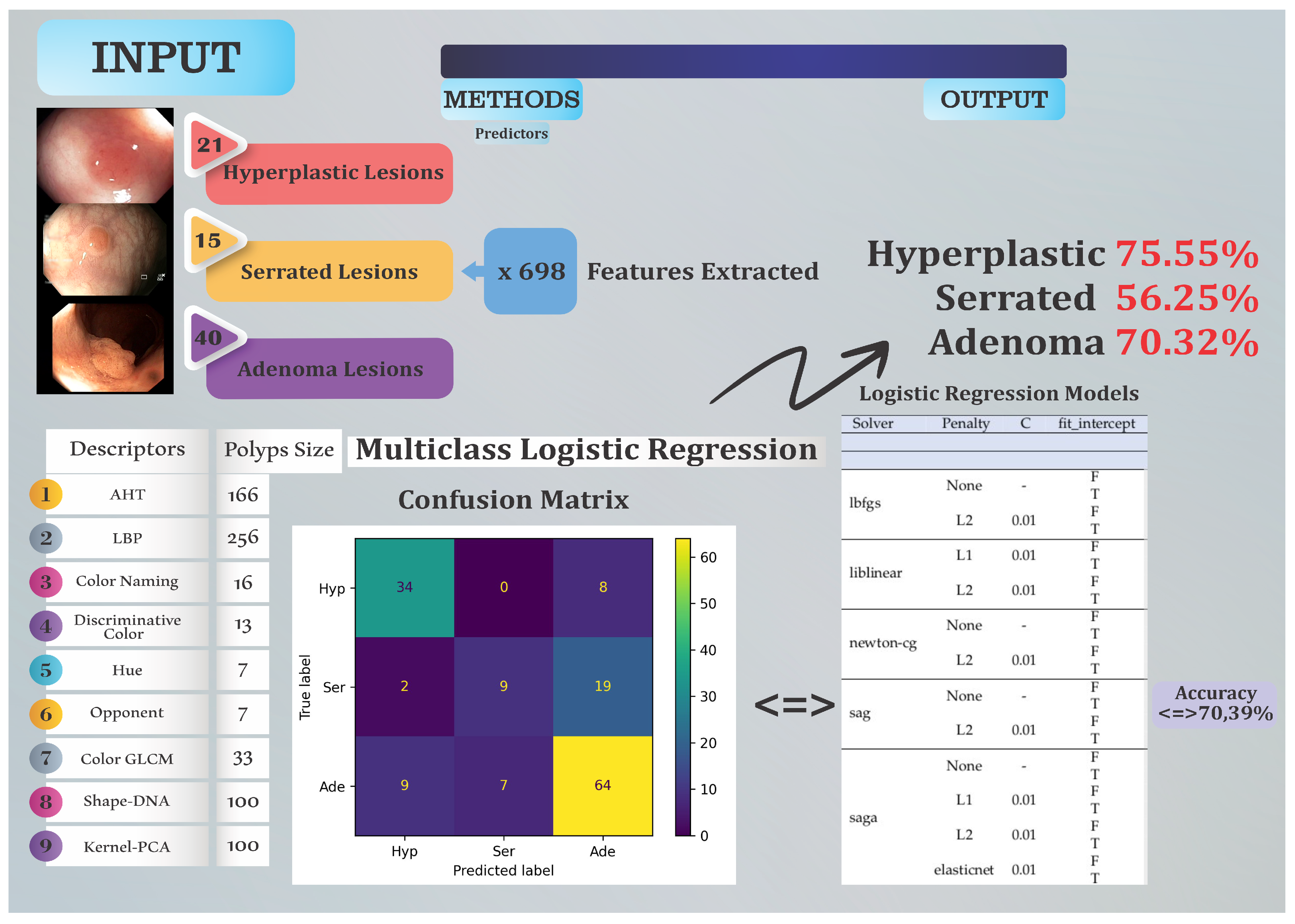
To check the influence of the data mix on the results obtained, for the two best models (LR with liblinear solver, L1 penalty and C = 0.01), we performed 2 x 50 runs for Fit_Intercept = False and Fit_Intercept = True, respectively, where random_state was equal 42, here we mixed randomly the rows of the dataset at every run.
An unpaired two-tailed T-test was applied, considering the significance level . I suggest presenting this as a decision rule, as cited in [47,48]. The p (p-value)=0.166, with p > , indicates no reason for rejecting the null hypothesis, indicating no statistical difference. The unpaired two-tailed T-test assumptions passed since both variables passed the normality assumption, verified using the Lilliefors test (P-value=0.2, 0.2>0.05) and the two sample variances were equally verified using the F-test (p=0.12, 0.12>0.05). The normality assumption was visually verified using the Q-Q plots.
Figure 4.
Q-Q Plots for visual validation of normality
4. Conclusions
Logistic Regression (LR) is easy to use and interpretable, making it a useful tool for initial exploratory analysis and for providing baseline performance metrics. Its efficiency in handling binary outcomes enables it to model the probability of polyp presence or absence based on extracted features from endoscopic images. However, the effectiveness of LR can be constrained by its inability to capture complex, non-linear relationships in high-dimensional medical image data.
In this study, we implemented and assessed the performance of LR algorithms for classifying gastrointestinal lesions, specifically utilizing the One-vs-Rest (OvR) and Multinomial LR classifiers for colon polyp image classification. Our findings demonstrate that while LR provides a useful starting point for such classification tasks, further exploration is needed to improve model accuracy and robustness.
Future research will focus on refining the methodology to better accommodate the complexities inherent in medical image data. This will include exploring advanced algorithms capable of capturing non-linear relationships and integrating additional features that may enhance predictive performance.
Moreover, it is essential to summarize the methodologies employed in this study, particularly those based on the works of [46,47,48,49,50], as these approaches have often been overlooked or misrepresented in existing literature. Addressing this aspect can lead to more robust research practices and prevent the publication of misleading findings, even in reputable journals. By emphasizing methodological clarity, we can contribute to more reliable outcomes in future studies involving medical imaging.
In the future, the next step is to refine its implementation, as a 3D reconstruction and classification tool would be very helpful for in-the-moment discussions on the removal of anomalous polyps (e.g., concave-shaped and suspected of deep neoplastic invasion). Improvements in lesion classification may help by collecting more lesion data, such as lesion dimensions or placement, and by asking about and taking into account the opinions of doctors. Deep Learning algorithms combined with the development of a useful tool for use in real-world colonoscopies may improve colonoscopy results and progress the field of gastrointestinal medicine. Investigating more complex methods, such as general-purpose GPU programming, may accelerate processing and allow for real-time diagnostics.
Author Contributions
Conceptualization, I.S., I.-L.B.; methodology, I.S., I.-L.B.; software, I.S., C.-D.M; validation, I.S., C.-D.M., I.-L.B.; formal analysis, I.S., C.-D.M. and I.-L.B.; investigation, I.S., C.-D.M., I.-L.B.; resources, I.S.; data curation, I.S.; writing—original draft preparation, C.-D.M., I.S. and I.-L.B.; writing—review and editing, C.-D.M and I.-L.B.; visualization, I.S., C.-D.M.; supervision, I.-L.B.; project administration, I.S. and C.-D.M.; funding acquisition, C.-D.M. All authors have read and agreed to the published version of the manuscript.
Funding
This research received no external funding.
Institutional Review Board Statement
Not applicable.
Data Availability Statement
The dataset consists of 152 brief colonoscopy videos, 152 photos (768 × 576 pixels) and 698 features extracted from every photo, all of which are available at https://www.depeca.uah.es/colonoscopy_dataset/. These data originate from real colonoscopy procedures, providing authentic and clinically relevant visual and feature-based information for research and analysis.
Acknowledgments
We acknowledge the support from the Romanian Ministry of Education, under contract no. 4067/2024, and of the University ’1 Decembrie 1918’ of Alba Iulia https://en.uab.ro/centre/1-center-for-scientific-research/. We thank the Research Center on Artificial Intelligence, Data Science, and Smart Engineering (ARTEMIS), from George Emil Palade University of Medicine, Pharmacy, Science and Technology of Târgu Mureș, Romania for the support of research infrastructure. Additionally, we acknowledge the support from the COST Action CA22137, Randomised Optimisation Algorithms Research Network (ROAR-NET), which facilitated collaboration and exchange of knowledge among researchers in this field. The authors thank Simona Ispas, who is responsible for graphic design.
Conflicts of Interest
The authors declare no conflicts of interest. The funders had no role in the design of the study; in the collection, analyses, or interpretation of data; in the writing of the manuscript; or in the decision to publish the results.
References
- Bray, F.; Ferlay, J.; Soerjomataram, I.; Siegel, R.L.; Torre, L.A.; Jemal, A. Global cancer statistics 2018: GLOBOCAN estimates of incidence and mortality worldwide for 36 cancers in 185 countries. CA: A cancer journal for clinicians 2018, 68, 394–424, Erratum in: CA Cancer J Clin. 2020 Jul;70(4):313. [Google Scholar] [CrossRef] [PubMed]
- Sung, H.; Ferlay, J.; Siegel, R.L.; Laversanne, M.; Soerjomataram, I.; Jemal, A.; Bray, F. Global Cancer Statistics 2020: GLOBOCAN Estimates of Incidence and Mortality Worldwide for 36 Cancers in 185 Countries. CA: A cancer journal for clinicians 2021, 71, 209–249. [Google Scholar] [CrossRef] [PubMed]
- Kim, H.J.; Parsa, N.; Byrne, M.F. The role of artificial intelligence in colonoscopy. Seminars in Colon and Rectal Surgery 2024, 35, 101007, Technologic Advances in Colon and Rectal Surgery. [Google Scholar] [CrossRef]
- Biffi, C.; Antonelli, G.; Bernhofer, S.; Hassan, C.; Hirata, D.; Iwatate, M.; Maieron, A.; Salvagnini, P.; Cherubini, A. REAL-Colon: A dataset for developing real-world AI applications in colonoscopy. ArXiv 2024. abs/2403.02163. [Google Scholar] [CrossRef]
- Jiang, J.; Xie, Q.; Cheng, Z.; Cai, J.; Xia, T.; Yang, H.; Yang, B.; Peng, H.; Bai, X.; Yan, M.; Li, X.; Zhou, J.; Huang, X.; Wang, L.; Long, H.; Wang, P.; Chu, Y.; Zeng, F.; Zhang, X.; Wang, G.; Zeng, F. AI based colorectal disease detection using real-time screening colonoscopy. Precis Clin Med 2021, 4, 109–118. [Google Scholar] [CrossRef] [PubMed]
- Lin, J.S.; Piper, M.A.; Perdue, L.A.; Rutter, C.M.; Webber, E.M.; O’Connor, E.; Smith, N.; Whitlock, E.P. Screening for Colorectal Cancer: Updated Evidence Report and Systematic Review for the US Preventive Services Task Force. JAMA 2016, 315, 2576–2594. [Google Scholar] [CrossRef]
- Adadi, A.; Adadi, S.; Berrada, M. Gastroenterology Meets Machine Learning: Status Quo and Quo Vadis. Advances in Bioinformatics 2019, 2019, 1870975. [Google Scholar] [CrossRef]
- Rasouli, P.; Dooghaie Moghadam, A.; Eslami, P.; Aghajanpoor Pasha, M.; Asadzadeh Aghdaei, H.; Mehrvar, A.; Nezami-Asl, A.; Iravani, S.; Sadeghi, A.; Zali, M.R. The role of artificial intelligence in colon polyps detection. Gastroenterology and Hepatology from Bed to Bench 2020, 13, 191–199. [Google Scholar] [CrossRef]
- Fati, S.M.; Senan, E.M.; Azar, A.T. Hybrid and Deep Learning Approach for Early Diagnosis of Lower Gastrointestinal Diseases. Sensors 2022, 22. [Google Scholar] [CrossRef]
- Galdran, A.; Carneiro, G.; Gonzalez Ballester, M.A., Double Encoder-Decoder Networks for Gastrointestinal Polyp Segmentation; 2021; pp. 293–307. [CrossRef]
- Lewis, J.; Cha, Y.; Kim, J. Dual encoder–decoder-based deep polyp segmentation network for colonoscopy images. Sci Rep 2023, 13, 1183. [Google Scholar] [CrossRef]
- ELKarazle, K.; Raman, V.; Then, P.; Chua, C. Detection of Colorectal Polyps from Colonoscopy Using Machine Learning: A Survey on Modern Techniques. Sensors 2023, 23. [Google Scholar] [CrossRef] [PubMed]
- Tian, Y.; Zorron Cheng Tao Pu, L.; Liu, Y.; Maicas, G.; Verjans, J.W.; Burt, A.D.; Shin, S.H.; Singh, R.; Carneiro, G. Chapter 15 - Detecting, localizing and classifying polyps from colonoscopy videos using deep learning. In Deep Learning for Medical Image Analysis (Second Edition), Second Edition ed.; Zhou, S.K.; Greenspan, H.; Shen, D., Eds.; The MICCAI Society book Series, Academic Press, 2024; pp. 425–450. [CrossRef]
- Mesejo, P.; Pizarro, D.; Abergel, A.; Rouquette, O.; Beorchia, S.; Poincloux, L.; Bartoli, A. Computer-Aided Classification of Gastrointestinal Lesions in Regular Colonoscopy. IEEE Transactions on Medical Imaging 2016, 35, 2051–2063. [Google Scholar] [CrossRef]
- V, P.; A, C.K.; Mubarak, D.N. Texture Feature Based Colonic Polyp Detection And Classification Using Machine Learning Techniques. 2022 International Conference on Innovations in Science and Technology for Sustainable Development (ICISTSD), 2022, pp. 359–364. [CrossRef]
- Li, W.; Yang, C.; Liu, J.; Liu, X.; Guo, X.; Yuan, Y. Joint Polyp Detection and Segmentation with Heterogeneous Endoscopic Data. Proceedings of the 3rd International Workshop and Challenge on Computer Vision in Endoscopy (EndoCV 2021): Co-located with the 18th IEEE International Symposium on Biomedical Imaging (ISBI 2021) 2021, 2886, 69–79.
- Galić, I.; Habijan, M.; Leventić, H.; Romić, K. Machine Learning Empowering Personalized Medicine: A Comprehensive Review of Medical Image Analysis Methods. Electronics 2023, 12. [Google Scholar] [CrossRef]
- Mongo-Onkouo, A.; Ikobo, L.; Apendi, C.; Monamou, J.; Gaporo, N.; Gassaye, D.; Mouakosso, M.; Adoua, C.; Ibara, B.; Ibara, J. Assessment of Practice of Colonoscopy in Pediatrics in Brazzaville, Congo. Open Journal of Pediatrics 2022, 12, 577–581. [Google Scholar] [CrossRef]
- Chen, S.; Lu, S.; Tang, Y.; Wang, D.; Sun, X.; Yi, J.; Liu, B.; Cao, Y.; Chen, Y.; Liu, X. A Machine Learning-Based System for Real-Time Polyp Detection (DeFrame): A Retrospective Study. Frontiers in Medicine 2022, 9, 852553. [Google Scholar] [CrossRef]
- Gono, K.; Obi, T.; Yamaguchi, M.; Ohyama, N.; Machida, H.; Sano, Y.; Yoshida, S.; Hamamoto, Y.; Endo, T. Appearance of enhanced tissue features in narrow-band endoscopic imaging. Journal of biomedical optics 2004, 9, 568–577. [Google Scholar] [CrossRef]
- Li, L.; Chen, Y.; Shen, Z.; others. Convolutional neural network for the diagnosis of early gastric cancer based on magnifying narrow band imaging. Gastric Cancer 2020, 23, 126–132. [CrossRef]
- Patino-Barrientos, S.; Sierra-Sosa, D.; Garcia-Zapirain, B.; Castillo-Olea, C.; Elmaghraby, A. Kudo’s Classification for Colon Polyps Assessment Using a Deep Learning Approach. Applied Sciences 2020, 10. [Google Scholar] [CrossRef]
- in the Paris Workshop, P. The Paris endoscopic classification of superficial neoplastic lesions: Esophagus, stomach, and colon. Gastrointestinal Endoscopy 2003, 58, S3–S43. [Google Scholar] [CrossRef]
- Ribeiro, H.; Libânio, D.; Castro, R.; Ferreira, A.; Barreiro, P.; Boal Carvalho, P.; Capela, T.; Pimentel-Nunes, P.; Santos, C.; Dinis-Ribeiro, M. Reliability of Paris Classification for superficial neoplastic gastric lesions improves with training and narrow band imaging. Endoscopy international open 2019, 7, E633–E640. [Google Scholar] [CrossRef]
- Ba, Q.; Yuan, X.; Wang, Y.; Shen, N.; Xie, H.; Lu, Y. Development and Validation of Machine Learning Algorithms for Prediction of Colorectal Polyps Based on Electronic Health Records. Biomedicines 2024, 12. [Google Scholar] [CrossRef]
- Cincar, K.; Sima, I. Machine Learning algorithms approach for Gastrointestinal Polyps classification. International Conference on INnovations in Intelligent SysTems and Applications, INISTA 2020, Novi Sad, Serbia, August 24-26, 2020; Ivanovic, M.; Yildirim, T.; Trajcevski, G.; Badica, C.; Bellatreche, L.; Kotenko, I.V.; Badica, A.; Erkmen, B.; Savic, M., Eds. IEEE, 2020, pp. 1–6. [CrossRef]
- Wei, M.; Fay, S.; Yung, D.; Ladabaum, U.; Kopylov, U. Artificial Intelligence–Assisted Colonoscopy in Real-World Clinical Practice: A Systematic Review and Meta-Analysis. Clinical and Translational Gastroenterology 2023, 15. [Google Scholar] [CrossRef]
- Riaz, F.; Silva, F.B.; Ribeiro, M.D.; Coimbra, M.T. Invariant Gabor Texture Descriptors for Classification of Gastroenterology Images. IEEE Transactions on Biomedical Engineering 2012, 59, 2893–2904. [Google Scholar] [CrossRef]
- van de Weijer, J.; Schmid, C. Coloring Local Feature Extraction. In Computer Vision – ECCV 2006; Leonardis, A., Bischof, H., Pinz, A., Eds.; Springer Berlin Heidelberg: Berlin, Heidelberg, 2006; pp. 334–348. [Google Scholar]
- Khan, R.; van de Weijer, J.; Khan, F.S.; Muselet, D.; Ducottet, C.; Barat, C. Discriminative Color Descriptors. 2013 IEEE Conference on Computer Vision and Pattern Recognition, 2013, pp. 2866–2873.
- van de Weijer, J.; Schmid, C.; Verbeek, J.; Larlus, D. Learning Color Names for Real-World Applications. IEEE Transactions on Image Processing 2009, 18, 1512–1523. [Google Scholar] [CrossRef]
- Hartley, R.; Zisserman, A. Multiple View Geometry in Computer Vision, 2 ed.; Cambridge University Press, 2004. [CrossRef]
- Reuter, M.; Peinecke, N.; Wolter, F.E. Laplace–Beltrami spectra as ‘Shape-DNA’ of surfaces and solids. Computer-Aided Design 2006, 38, 342–366. [Google Scholar] [CrossRef]
- Bishop, C.M. Pattern Recognition and Machine Learning (Information Science and Statistics); Springer-Verlag: Berlin, Heidelberg, 2006. [Google Scholar]
- Russell, S.; Norvig, P. Artificial Intelligence: A Modern Approach, 3 ed.; Prentice Hall, 2010.
- James, G.; Witten, D.; Hastie, T.; Tibshirani, R. An Introduction to Statistical Learning: With Applications in R; Springer: New York, 2013. [Google Scholar]
- Byrd, R.H.; Lu, P.; Nocedal, J.; Zhu, C. A Limited Memory Algorithm for Bound Constrained Optimization. SIAM Journal on Scientific Computing 1995, 16, 1190–1208. [Google Scholar] [CrossRef]
- Zhu, C.; Byrd, R.H.; Lu, P.; Nocedal, J. Algorithm 778: L-BFGS-B: Fortran subroutines for large-scale bound-constrained optimization. ACM Trans. Math. Softw. 1997, 23, 550–560. [Google Scholar] [CrossRef]
- Morales, J.L.; Nocedal, J. Remark on “algorithm 778: L-BFGS-B: Fortran subroutines for large-scale bound constrained optimization”. ACM Trans. Math. Softw. 2011, 38. [Google Scholar] [CrossRef]
- Friedman, J.; Hastie, T.; Tibshirani, R. Regularization paths for generalized linear models via coordinate descent. Journal of Statistical Software 2010, 33, 1–22. [Google Scholar] [CrossRef]
- Tay, J.K.; Narasimhan, B.; Hastie, T. Elastic net regularization paths for all generalized linear models. Journal of Statistical Software 2023, 106, 1, Epub 2023 Mar 23. [Google Scholar] [CrossRef]
- Schmidt, M.; Le Roux, N.; Bach, F. Minimizing finite sums with the stochastic average gradient. Mathematical Programming 2017, 162, 83–112. [Google Scholar] [CrossRef]
- Defazio, A.; Bach, F.R.; Lacoste-Julien, S. SAGA: A Fast Incremental Gradient Method With Support for Non-Strongly Convex Composite Objectives. Neural Information Processing Systems, 2014.
- Singh, D.; Singh, B. Feature wise normalization: An effective way of normalizing data. Pattern Recognition 2021, 122, 108307. [Google Scholar] [CrossRef]
- Pedregosa, F. and Varoquaux, G. and Gramfort, A. and Michel, V. and Thirion, B. and Grisel, O. and Blondel, M. and Prettenhofer, P. and Weiss, R. and Dubourg, V. and Vanderplas, J. and Passos, A. and Cournapeau, D. and Brucher, M. and Perrot, M. and Duchesnay, E.. Scikit-learn: Machine Learning in Python. Journal of Machine Learning Research 2011, 12, 2825–2830.
- Iantovics, Enăchescu, C. Method for Data Quality Assessment Synthetic Industrial Data. Sensors 2022, 22, 1608. [CrossRef]
- Iantovics, L.B.; Rotar, C.; Nechita, E. A Novel Robust Metric for Comparing the Intelligence of Two Cooperative Multiagent Systems. Procedia Computer Science 2016, 96, 637–644, Knowledge-Based and Intelligent Information & Engineering Systems: Proceedings of the 20th International Conference KES-2016. [Google Scholar] [CrossRef]
- Iantovics, L.B. Measuring Machine Intelligence Using Black-Box-Based Universal Intelligence Metrics. New Approaches for Multidimensional Signal Processing; Kountchev, R., Mironov, R., Nakamatsu, K., Eds.; Springer Nature Singapore: Singapore, 2023; pp. 65–78. [Google Scholar]
- Iantovics, L.B.; Dehmer, M.; Emmert-Streib, F. MetrIntSimil—An Accurate and Robust Metric for Comparison of Similarity in Intelligence of Any Number of Cooperative Multiagent Systems. Symmetry 2018, 10. [Google Scholar] [CrossRef]
- Iantovics, L.B. Black-Box-Based Mathematical Modelling of Machine Intelligence Measuring. Mathematics 2021, 9. [Google Scholar] [CrossRef]
Figure 2.
Example of gastrointestinal polyps
Figure 3.
Confusion Matrix for the best model
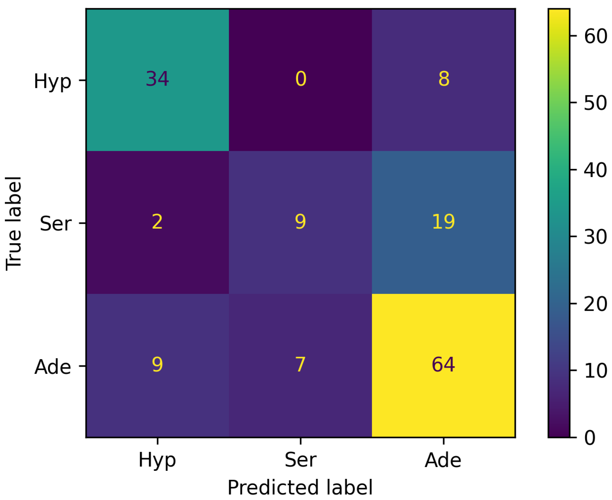

Table 1.
Confusion Matrix for Binary classification
| Predicted P (1) | Predicted N (0) | |
|---|---|---|
| Real P (1) | TP | FN |
| Real N (0) | FP | TN |
Table 2.
Confusion Matrix for 3-class classification
| Predicted Class A | Predicted Class B | Predicted Class C | |
|---|---|---|---|
| Real Class A | |||
| Real Class B | |||
| Real Class C | |||
Table 3.
Logistic Regression - Hyperparameters tuning
| Hyperparameter | Values Considered |
|---|---|
| data type | { non-normalised, normalised } |
| multi_class type | { multinomial, ovr } |
| solver | { lbfgs, liblinear, newton-cg, sag, saga } |
| penalty | { none, L1, L2, elasticnet } |
| C | { 0.01, 0.1, 1, 10, 100 } |
| fit_intercept | { False, True } |
| max_iter | { 100, 150, 200, 250, 300, 1000, 5000, 10000 } |
| l1_ratio | { 0.5 } |
Table 4.
Performance of Logistic Regression Models
| Solver | Penalty | C | fit_intercept | Accuracy (Std Dev) [%] | |||
|---|---|---|---|---|---|---|---|
| OvR | Multinomial | ||||||
| non-Norm | Norm | non-Norm | Norm | ||||
| lbfgs | None | - | F | Not conv | Not conv | 61.18 (3.42) | Not conv |
| T | Not conv | Not conv | 66.45 3.42 | Not conv | |||
| L2 | 0.01 | F | 63.82 (2.87) | 52.63 (4.16) | 62.5 (3.89) | 52.63 (4.16) | |
| T | 63.82 (2.87) | 52.63 (4.16) | 61.84 (4.36) | 52.63 (4.16) | |||
| liblinear | L1 | 0.01 | F | 70.39 (3.89) | 27.63 (5.42) | ||
| T | 70.39 (3.89) | 27.63 (5.42) | |||||
| L2 | 0.01 | F | 63.16 (3.22) | 52.63 (4.16) | |||
| T | 63.16 (3.22) | 52.63 (4.16) | |||||
| newton-cg | None | - | F | 55.92 (10.59) | 45.39 (1.14) | 60.53 (4.92) | 36.84 (2.63) |
| T | 63.16 (1.86) | 40.79 (2.28) | 59.87 (5.05) | 42.76 (6.8) | |||
| L2 | 0.01 | F | 63.82 (2.87) | 52.63 (4.16) | 62.5 (3.89) | 52.63 (4.16) | |
| T | Not conv | 52.63 (4.16) | 63.82 (3.89) | 52.63 (4.16) | |||
| sag | None | - | F | 63.82 (2.18) | 40.13 (5.9) | 63.82 (1.14) | 38.16 (6.03) |
| T | 63.82 (2.18) | 42.11 (5.58) | 63.82 (1.14) | 40.79 (5.43) | |||
| L2 | 0.01 | F | 63.82 (2.18) | 52.63 (4.16) | 63.82 (1.14) | 52.63 (4.16) | |
| T | 63.82 (2.18) | 52.63 (4.16) | 63.82 (1.14) | 52.63 (4.16) | |||
| saga | None | - | F | 63.16 (4.16) | 44.08 (6.8) | 62.5 (2.18) | 41.45 (7.06) |
| T | 63.16 (4.16) | 43.42 (9.39) | 62.5 (2.18) | 44.08 (7.76) | |||
| L1 | 0.01 | F | 62.5 (3.89) | 27,63 (5.42) | 61.18 (1.14) | 27.63 (5.42) | |
| T | 62.5 (3.89) | 52.63 (4.16) | 61.18 (1.14) | 52.63 (4.16) | |||
| L2 | 0.01 | F | 63.16 (4.16) | 52.63 (4.16) | 62.5 (2.18) | 52.63 (4.16) | |
| T | 63.16 (4.16) | 52.63 (4.16) | 62.5 (2.18) | 52.63 (4.16) | |||
| elasticnet | 0.01 | F | 63.16 (4.92) | 27.63 (5.42) | 61.18 (1.14) | 27.63 (5.42) | |
| T | 63.16 (4.92) | 52.63 (4.16) | 61.18 (1.14) | 52.63 (4.16) | |||
Table 5.
Comparative performance
| LR | Mesejo2016 | Human Expert | Human Beginner | |
|---|---|---|---|---|
| Acc Mean | 70.39% | 65.00% | 58.42% | |
| Acc Max | 76.32% | 76.69% | - | - |
| Prec Hyp | 75.55% | 66.66% | 62.00% | 66.26% |
| Prec Ser | 56.25% | 69.23% | 52.20% | 51.54% |
| Prec Ade | 70.32% | 80.55% | 73.50% | 66.65% |
| Recall Hyp | 80.95% | 85.71% | 67.90% | 52.40% |
| Recall Ser | 30.00% | 60.00% | 63.75% | 44.70% |
| Recall Ade | 80.00% | 72.50% | 63.75% | 25.00% |
| F1 Hyp | 78.16% | 74.99% | 64.82% | 58.52% |
| F1 Ser | 39.13% | 64.29% | 57.40% | 47.88% |
| F1 Ade | 74.85% | 76.31% | 68.28% | 36.36% |
| macro_av Pre | 67.37% | 72.15% | 62.57% | 61.48% |
| macro_av Recall | 63.65% | 72.74% | 65.13% | 40.70% |
| macro_av F1 | 64.05% | 71.86% | 63.50% | 47.59% |
Disclaimer/Publisher’s Note: The statements, opinions and data contained in all publications are solely those of the individual author(s) and contributor(s) and not of MDPI and/or the editor(s). MDPI and/or the editor(s) disclaim responsibility for any injury to people or property resulting from any ideas, methods, instructions or products referred to in the content. |
© 2024 by the authors. Licensee MDPI, Basel, Switzerland. This article is an open access article distributed under the terms and conditions of the Creative Commons Attribution (CC BY) license (http://creativecommons.org/licenses/by/4.0/).
Copyright: This open access article is published under a Creative Commons CC BY 4.0 license, which permit the free download, distribution, and reuse, provided that the author and preprint are cited in any reuse.


