
Submitted:
11 December 2024
Posted:
12 December 2024
You are already at the latest version
Abstract
The Patient Rule Induction Method (PRIM) is a data mining technique used for identifying patterns in datasets, particularly focusing on discovering regions of the chosen input space where the response variable is unusually high or low. It falls in the subgroup Discovery field, where finding small groups is more relevant for the explainability of the results, although it is not a classification technique per se. In this paper, we introduce a new Framework for the breast cancer classification based on PRIM. This new method involves, first, the random choice of different input space for each class label. Second, the organization and the pruning of the rules using the Metarules. And finally, it also includes the proposition of a way to handle the class overlapping and, hence, define the final classifier. The Framework is tested on five real-live breast cancer datasets and compared to 3 often used algorithms for breast cancer classification: XG Boost, Logistic Regression and Random Forest. Across the four metrics and datasets, both our PRIM-based Framework and Random Forest demonstrate robust performance, with our framework showing notable accuracy and recall. XGBoost maintains strong F1-scores across the board, indicating balanced precision and recall. In the other hand Logistic Regression, while competent, generally underperforms compared to the other algorithms, especially in terms of accuracy and recall, achieving 94.1% accuracy against 96.8% and 85.4% recall against 94.2% for the PRIM-based framework on the Wisconsin dataset.
Keywords:
Breast Cancer
; Machine Learning
; Bump Hunting
; Patient Rule Induction Method
; Explainability
1. Introduction
Machine Learning has been applied to several fields, the medical one is considered the most delicate since it interferes in the life of patients. Breast cancer is the most prevalent cancer among women. Compared to other cancer types, breast cancer has a comparatively low mortality rate. It does, however, have the greatest fatality rate of any cancer in women due to the huge number of incidences [35]. For survival, early diagnosis is essential. Lack of funding and undeveloped healthcare infrastructures, especially in developing countries, make it challenging for patients to see a doctor. The patient survival rate can be improved by creating early diagnosis programs based on early indications and symptoms, hence the need for explainable supervised machine learning models for the classification of breast cancer patients and the identification of condition that explain different breast cancer patient classes. To this end, the objective of this paper is to introduce a new framework for explainable breast cancer classification based on an adapted version of PRIM, a bump hunting algorithm [14].
Even though scientists have worked on improving the accuracy of ML models, explainability remains necessary to help practitioners in their decision-making process. Current research has focused on making the models understandable and usable [26]. In [27] authors give a review on explainable artificial intelligence (AI) and accentuate the focus lately on this field involving the interaction with humans.
In this context, it is essential to focus on both sides: the high accuracy of the model and the explainable and interpretable results. One of the approaches that have been constructed to deal with the research in an input space of interesting groups and behave well in high dimensional data is bump hunting. Introduced by Friedman and Fisher [14], the Patient Rule Induction Method is a bump hunting algorithm that consists of searching at each iteration for the most optimal rule. Since it peels one dimension at a time, it constructs at the end a rule shaped as a box, hence the term box induction used in the literature. PRIM is not a classification method. The output is a set of rules corresponding to one class, it is, therefore a powerful data mining procedure to explore the dataset. We have chosen to adapt this method, in a way to build an interpretable and explainable classifier in different types of breast cancer classification problems.
To this end, we introduce, in this paper, a framework for Breast Cancer classification based on an adaptation of the Patient Rule Induction Method handling both categorical and numeric features. The suggested framework, allows to build classification models that are as accurate as cutting-edge ensemble techniques while still being easy to understand and explain. Indeed, discovering new subgroups in the data space could lead, in this medical field, to new insights for the breast cancer diagnosis and prognosis problems.
In the proposed framework for breast cancer classification, we run for each class several iterations of PRIM algorithm on random subsets of features to find all the rules, then cross validation is used to select the rules to produce the correct classifier for each dataset. Finally, the resulting classification rules are organized and pruned using Metarules [17]. At this level we identify containment between the rules of the same class and identify the overlapping regions between the rules representing different classes.
The rest of the paper is organized as follows. In the next section we review briefly the prediction of breast cancer using machine learning. Then we present the three algorithms for classification selected to be part of the comparison with the adapted PRIM, namely: Random Forest, XGBoost and Logistic Regression. We explain, after, the Patient Rule Induction Method, its functioning and why it is more interesting to work with a bump hunting method in the medical field. In Section 3 we explain in details the framework proposed for breast cancer classification. We review the methods to validate a classifier, the way to handle rule conflict and explain how metarules allow for pruning redundant and irrelevant rules. An empirical evaluation follows in Section 4 and Section 5 including the limitations of the work, and finally in Section 6 we provide the discussion and the conclusion.
2. Material and Methods
In this section we start by explaining how breast cancer classification is handled in the literature. This allowed us to identify three major supervised learning algorithms used for this classification problem, namely Random Forest [12], XGBOOST [11] and Logistic Regression [13] for which we give an overview in section 2.2. Finally, we present the PRIM algorithm as it is an essential ingredient in our framework and provide a literature review of PRIM’s applications which indicates its popularity of medical application.
2.1. State-of-the Art of Breast Cancer Classification
Breast cancer is very popular among cancer prediction in machine learning. Several researchers have developed and implemented techniques over the years to look up for new patient profiles or features combination that can lead medical teams to a better breast cancer detection [22]. In this section we present several relevant papers related to using machine learning algorithms to predict breast cancer in order to determine the algorithms to adopt for our empirical study. More detailed reviews can be found in [36,37,38].
Authors in [1] have investigated breast cancer in Chinese women by looking at the signs before the symptoms are even shown. It has been shown that it is as successful as the accuracy of the prediction model used for the screening. The article evaluates and compares the performance of four ML algorithms: XGBoost, Random Forest, Deep Neutral Network and Logistic Regression, on predicting breast cancer. The model training was performed using a dataset consisting of 7127 breast cancer cases and 7127 matched healthy controls, while the performance was measured based on AUC, sensitivity, specificity, and accuracy following a repeated 5-fold cross-validation procedure. The results showed that all three novel ML algorithms outperformed Logistic Regression in terms of discriminatory accuracy in identifying women at high risk of cancer. XGBoost also proved to be the best to develop a breast cancer model using breast cancer risk factors.
Five ML algorithms were applied to the breast cancer Wisconsin Diagnostic dataset in [2], in order to determine which are the best and most effective in terms of accuracy, confusion matrix, AUC, sensitivity and precision, to predict and diagnose breast cancer.The algorithms used for the study are: SVM, Random Forests, Logistic Regression, Decision Tree, K-NN. Comparing the results shown that SVM scored a higher efficiency of 97.2%, with a precision of 97.5 and UAC of 96.6% and outperformed the rest of the algorithms.
Authors in [3] conducted a study to evaluate and compare 8 ML learning algorithms: Gaussian Naïve Bayes (GNB), k-Nearest Neighbors (K-NN), Support Vector Machine (SVM), Random Forest (RF), AdaBoost, Gradient Boosting (GB), XGBoost, and Multi-Layer Perceptron (MLP). The algorithms were applied to Wisconsin Breast Cancer dataset, using and 5-folds cross-validation. XGBoost results show great performance and accuracy, concluding that the algorithm is the best to predict Breast Cancer in Wisconsin dataset, with an accuracy of 97.1%, recall of 96.75%, a precision of 97.28%, 96.99% for F1-score and 99.61% for AUC.
Three machine learning techniques for predicting breast cancer were used in [4]. The article aims to develop predictive models, for breast cancer recurrence in patients who followed-up for two years, by applying data mining techniques. The main goal was to compare the performance through sensitivity, specificity, and accuracy of well-known ML algorithms: Decision Tree, Support Vector Machine, and Artificial Neural Network algorithms.
The study was applied to a dataset of 1189 records, 22 predictor variables, and one outcome variable, using 10-fold cross-validation for measuring the unbiased prediction accuracy. Results shown that SVM classification model predicted breast cancer with least error rate and highest accuracy of 0.957, while the DT model was the lowest of all in terms of accuracy with 0.936, ANN scored 0.947.
To predict breast cancer metastasis in [5], the researchers used 4 ML algorithms: random forest, support vector machine, logistic regression, and Bayesian classification to evaluate serum human epidermal growth factor receptor 2 (sHER2) as part of a combination of clinicopathological features used to predict breast cancer metastasis. These algorithms were applied to a sample cohort that comprised 302 patients. Results show that random-forest-based model outperformed the rest of the algorithms, with an AUC value of 0.75(p < 0.001), an accuracy of 0.75, 0.80 of sensitivity, and specificity of 0.71.
2.2. Overview of Major Supervised Algorithms Used for Breast Cancer Classification
We have chosen to use three algorithms to compare it with our approach, namely Random Forest, Logistic Regression and XGBoost due to their recurring use in the literature for breast cancer classification and because they would give us an accurate evaluation of our algorithm.
XGBoost [11] is a supervised learning algorithm which principle is to combine the results of a set of simpler and weaker models to provide a better prediction. This method is called model aggregation. The idea is simple: instead of using a single model, the algorithm uses several in a sequential way and which will then be combined to obtain an aggregated model. It is above all, a pragmatic approach that allows to manage regression and classification problems. the algorithm works in a sequential way. Contrary to the Random Forest for example, this way of doing things will make it slower of course but it will especially allow the algorithm to improve itself by capitalizing on the previous executions. It starts by building a first model that it will evaluate. From this first evaluation, each individual will then be weighted according to the performance of the prediction.
Random Forest [12] is a tree-based classifier consisting of a large number of decision trees that operate as an ensemble. For classification tasks, the output of the random forest is the class selected by most trees. For regression tasks, the mean or average prediction of the individual trees is returned. It generates mostly black box models, and it is known for lacking in interpretability.
Logistic Regression [13] is a supervised method that is used for classification problems. Logistic Regression predicts the probability of an event or class that is dependent on other factors, therefore the output is always between 0 and 1. It is a very commonly used algorithm for constructing predictive models in the medical field.
2.3. The Patient Rule Induction Method
2.3.1. Overview
In a supervised learning environment, the Patient Rule Induction Method [14] is a bump hunting algorithm that locates areas in the input variables subspace, selected by the decision maker, that are connected to the highest or lowest occurrence of a target label of a class variable.
Two steps make up the Patient Rule Induction Method. The first phase is the top-down peeling, where the boxes are built and each box is bounded by the variables defining the selected subspace, given a subset of the input variables subspace. The data analyst may control how much data is eliminated at each peel; typically, this amount is 5%, thus the name "patient." Due to earlier decisions made out of suboptimal greed, the final box discovered after the peeling process could not be ideal.
The boxes are extended by repeatedly extending their bounds as long as the result's density grows in the second PRIM phase, known as the bottom up pasting. Figure 1 shows PRIM's method for locating a box in the initial stage of top-down peeling. Up until halting requirements are met, these two procedures are continued iteratively to locate further areas. PRIM is a greedy algorithm as a result. A collection of boxes or regions that provide rules connecting the targeted label of the dependent variable to the explanatory qualities in the data subspace initially selected by the analysts are the result of PRIM.
Even if the resulting areas and rules are actionable, the selection of variables can consistently alter the answer to the original problem since the search dimension is decided by a human component, making it possible to ignore important rules while attempting to forecast a phenomenon.
2.3.2. Related Work
Numerous applications of PRIM are available in the literature. The Patient Rule Induction Method for parameter estimation (PRIM-PE) is one of them [30]. Due to over-parameterization and a lack of knowledge, it is advantageous to locate every behavioral parameter vector that might possibly exist when using hydrologic models, according to the authors. The patient rule induction method for parameter estimation (PRIM-PE) is a novel method developed. It identifies all areas of the parameter space that have a model behavior that is acceptable. The response surface is adequately represented by the parameter sample created by the authors, which has a uniform distribution inside the "good-enough" area. The area in the parameter space where the acceptable parameter vectors are found is then defined using PRIM. Markov chain Monte Carlo sampling was contrasted with PRIM-PE sampling. The approach worked well, successfully capturing the desirable areas of the parameter space.
For finding the multidimensional tradeoffs between coverage, density, and interpretability, another work [31] proposes then contrasts a many-objective optimization strategy with an upgraded usage of PRIM. Although this method is marginally superior to the enhanced PRIM version, they qualitatively identify the same subspaces, according to the article. The method addresses other pertinent issues including consistency and variety, prevents overfitting, and facilitates the use of more complex metaheuristic optimization techniques for scenario discovery.
The authors of [32] have suggested a technique for analyzing huge data using PRIM. The first stage entails using PRIM to create an area that has a subset with the greatest output variable using chosen input variables and output variables. Aggregating, sorting, comparing, and calculating new metrics make up the second stage. A different option is to decrease the subset using the weighted item set function, then use the smaller subset in online analytical processing to look for patterns. In [33], the researchers use a modified PRIM to try to statistically identify significant subgroups based on clinical and demographic characteristics. The results were satisfactory enough to draw the conclusion that the data can be used to understand why the clinical trial failed and to aid with the design of subsequent studies. You can find other literature reviews in [20,34] that show the advantage of working with PRIM, which the exploration of all the feature space until discovering the smallest subgroups that can create a tendency for our target variable, to large group that can explain quickly a phenomenon. The literature has also shown that PRIM performs better than CART in several cases since CART can peel up to 50% of the data at each split. The use of a bump hunting procedure is not popular among the medical community, and this work aims to show the potential of a new interpretable approach.
To evaluate the interpretability of ML models, authors in [25] introduced 4 levels of interpretability in models. There are four different level of interpretability. Level 1 regroups all the approaches that gave only black box models, without any means to interpret the results as induced by Random Forest. The second level concerns the approaches in which the domain knowledge is part of the construction of the models, it participates in the design of the model and lead the algorithm toward the optimum model for the problem encountered. The third level concern not only the participation of the domain knowledge in the construction of the final model, but also the integration of tools to further improve the interpretability. In this level the interpretability and the explainability, since one concerns the clarity of the model and the other concerns the domain knowledge required. The final level, is the best level of interpretability, where the model is crystal clear to the experts. According to the paper PRIM is situated in level 4 because by choosing the input research space, and tuning the parameters according to the domain knowledge, PRIM provides the user with non-complex rules.
3. PRIM Based Framework for Breast Cancer Classification and Explanation
This section aims at presenting the proposed approach. Indeed, we detail the steps of the framework by explaining the procedure and giving each time reviews in the literature that guided us through the elaboration of the framework.
3.1. Presentation of the Framework
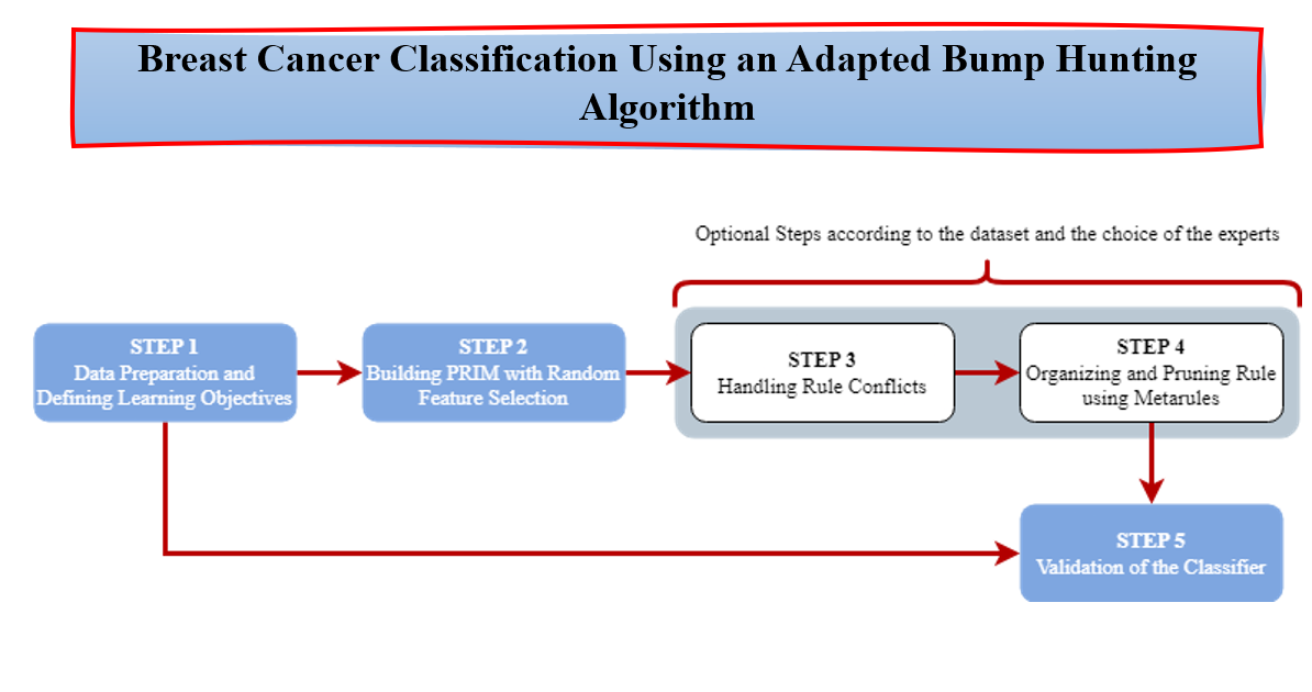
As uncovered previously in the literature review Section, PRIM is well adapted for medical field prediction by detecting interesting subgroups. Therefore, we introduce a PRIM based framework to build accurate, interpretable and explainable classifiers for breast cancer classification. The suggested framework used PRIM algorithm implemented on random selections of features. This allows the extraction of rules for all the class labels in the breast cancer dataset under consideration, according to a predefined support, peeling and pasting thresholds. In addition, the framework also contains a method to detect regions in the space where conflicting rules may overlap and a method to handle this rule conflicts. We also find in the framework a method to prune irrelevant rules that are usually redundant or contained in one another. Finally, the last step consists of validating the classifier of the breast cancer prediction. Figure 2, gives a display of the different steps contained in the proposed framework. Step 1 consists of the data preprocessing and the establishment of the learning objectives. Step 2 defines the rules generated by PRIM on random features. These two first steps are mandatory. Steps 3 and 4 are optional depending on the dataset and the objectives of the use but we highly recommend them to increase the interpretability and the explainability of the model. And finally Step 5 is where the classifier, hence the model, is validated. Hereafter, we develop the main steps of the proposed framework.
3.1.1. Step 1: Data Preparation and Defining Learning Objectives
The first step of the framework consists of the data preparation and the definition of the learning objectives. In fact, the learning objectives have to be set at first to allow an optimal choice of the thresholds and also orient more accurately feature engineering if needed. Indeed, data preprocessing is a necessary step in machine learning, but in our framework, the only data handled contains a target variable y often binary y = {0,1}. Survival analysis does not enter in the scope of our framework. According to the different applications in the literature review, there are two types of breast cancer dataset for classification: One with the target variable for whether the patient is dead or alive, and the other one for the type of the tumor if malignant or benign.
3.1.2. Step 2: Building the Boxes with PRIM on Random Feature Selection
As stated before, the biggest shortcomings for the use of PRIM as a classifier is the feature selection. Indeed, the choice of the input space does not lead to all the boxes, hence the rules, of interesting subgroups. In this context, we propose to run PRIM several time with a random feature choice for each class. Each time, PRIM will induce boxes and metrics that show whether the features selected are accurate for the real-life problem or not. Thus, increasing the discovery of interesting subgroups but also, and most importantly, the interpretability. In fact, most of the accurate algorithms generate black box models, leading experts to a completely non interpretable and hence useless models where optimizing becomes obligatory.
The algorithm developed extracts rules for each class separately. Each set of boxes induced by the random features for the class is stocked into a ruleset. Once the procedure is finished, the number of boxes obtained is considerable and does not define a classifier. We still have to diagnose overlapping regions and then prune rules using the metarules.
The version of PRIM we suggest build a classifier using random feature space. The dataset at the entry can have categorical or numeric attributes since they are both handled by PRIM. The target variable should be binary, if not we can divide the problem into sub problems. The algorithm requires also a minimum support, a peeling threshold and a pasting threshold. The algorithm starts by finding the rules for each class on the training set and then we move to the next step of the framework. According to the output, we can move directly to the fifth step to validate the classifier by cross-validation, or we can go through overlapping detection and pruning rules using metarules, which we recommend as we intend to build an interpretable and explainable model.
3.1.3. Step 3: Handling Rule Conflict
Rule conflict refers to the rules of different classes that can overlap in a region of the input space. The handling of the rule conflict, or also know as overlapping classes, is a big part of machine learning research since it changes the classification of some instances that fall into the overlapping regions [18,19,23,24].
Going through the literature of this area, we have found that the most used way to resolve the conflict, is to analyze the problem depending on the support of the conflicted region. If the region Rc is too small in comparison to the biggest one, as in case of Figure 3.a, then all the data that falls into it will be classified as the one of the biggest rules with the higher confidence and coverage. If the region of conflict Rc has a biggest support, which means more data points fall into it then into the other one that constitutes the conflicted region, as in Figure 3.b, then we should reconsider the classification and analyze the input space. And if the region has an average size in comparison with the ones that constitutes it, as in Figure 3.c, then we calculate which of the classes has the majority in the conflict region Rc.
The problem of overlapping classes often depends on the data and the sparsity of the points. There are no means to predict whether we will have class conflict or not. In the medical field, since the classification takes on a human dimension, we suggest providing the experts with the overlapping regions and let them decide, according to the issue, how to handle the conflict and if another classification is necessary.
3.1.4. Step 4: Organizing and Pruning Rules Using Metarules
Pruning in machine learning consists of reducing and/or organizing the ruleset to make it more interpretable. It is often used in black box models such as models induced by Random Forest. There are several pruning techniques: optimization, minimum support and metarules. Other pruning techniques can be found in [15,16]. We chose to use metarules [17] because it is the most adapted with our classifier. Indeed, we intend to organize the whole ruleset without removing any rule. The important side in our classifier is to give interpretable results.
The metarule is an association between one rule in the antecedent and another rule in the consequent. It can be discovered using association rules mining algorithm from a set of rules that share the same consequent of interest. In order to find all the associations between rules that share the same consequent, the support for metarules can be set to 0%, the confidence is specified by the user as in association rules mining. The uncovered metarules divide the rules into disjoint clusters of rules, each cluster covers a local region in the data space, which allows to reveal containment and overlap between rules that belong to each cluster. Figure 4 displays an example of how the rules are organized using metarules. Indeed, Rule 3 is contained into Rule 2, and Rule 4 is associated to Rule 5 and Rule 6 is associated to Rule 7. Therefore, the rules 3, 4 and 6 can be pruned because they are already represented respectively by the rules 2, 5 and 7.
3.1.5. Step 5: Validation of a Classifier
As we intend to create a classifier based on the boxes generated for each class by PRIM, which falls in the subgroup discovery algorithms we have investigated the statistical research field on the criterions and the tools to build a classifier. According to the original paper of the Classification and Regression Tree by Breiman et al [21], cross validation is the tool to validate the classifier. Hence, we use it in Step 5 to reinforce our model.
3.2. Illustrative Example of the PRIM Based Classification Framework
To illustrate how our framework works, we have applied it on the Diabetes Dataset available in the UCI Machine Learning Repository. The dataset consists of 768 instances, 8 attributes and two classes: 1 if the patient is diabetic and if 0 the patient is not diabetic.
Step 1: For this first step we will first generate random combination for the features. For the sake of proving the concept, we generated only 10 random combinations of attributes.
Step 2: The second step is to run PRIM on each combination for the diabetics first and then for the non-diabetics. We obtain a total of 56 rules for class 1 and 37 for class 0. We used the “prim” library from Python. Table 1 displays all the rules found for both classes and their characteristics: coverage, density (confidence), support and the dimension of the rules. A lower rule dimension allows for less complex rules which makes more actionable.
Step 3 & 4: The third step is to detect the overlapping classes using Metarules. For this, we have first set the matrix of instances where we cross instances with the rules, and then we apply association rules between the rules as explained in Figure 5. Thanks to this method we detect not only rules of class 1 that are associated with rules of class 0 but also contained rules for each class label. To implement the metarules, we work on Orange [28], with the package “association rule mining”. For the 56 rules for class = 1, we set the confidence threshold of the metarules at 90% and their support threshold at 0%, we found:
10 rules that were contained to each other
5 rules that are associated with other 5 rules
This pruned the ruleset for class 1 from 56 rules to 48 rules.
The same procedure was made for the class = 0 ruleset, moving from 37 rules to 21 rules because of the redundancy of some of them.
To detect the rule conflict, we use the same matrices but we look for association between the matrix in Figure 5.a and the one in Figure 5.b. In our example, due to the fact that we got some containment in the rules and redundancy, there is no major rule conflict. As we stated before, the class that has the majority in the region wins the conflict.
Step 5: The final step to construct the classifier is to perform cross-validation to retain the important rules that build the accurate model. We have performed a 5-fold cross validation. We obtained as an average accuracy of 95.63%, as an average recall of 89.43% and as an average precision of 92.8%. The rules obtained don’t exceed 4 features, they are not complex to read. Finally, a total of 70 rules for both classes were retained.
4. Experimental Setup for the Empirical Evaluation of the PRIM Based Framework for Breast Cancer Classification
This section aims at presenting the setting for the experiment with the details about the datasets and the material used to compute the empirical evaluation.
To evaluate the PRIM based framework, we conducted a comparative study for the classifier from our PRIM based framework against three classification algorithms for five real-life breast cancer datasets based on four measures to measure the performance of the classifiers namely: accuracy, precision, recall and F1-score.
The five breast cancer datasets used can be displayed in Table 2. Wisconsin is taken from the UCI Machine Learning Repository; SEER and the ISPY1-clinica datasets are both taken from the National Cancer Institute of USA and it gives as a target variable whether the patient is dead or alive according to some features. The NKI dataset has been published by the Netherland Cancer Institute and has 1570 column. Finally, the Mammographic-masses dataset has been published by the Image Processing and Medical Engineering Department (BMT) in Fraunhofer Institute for Integrated Circuits (IIS) in Germany. The datasets didn’t need preprocessing since PRIM can handle both categoric and numeric features, we therefore cleaned the missing values.
For the four algorithms we used a 10-fold cross-validation, and we relied on the accuracy to choose for each dataset the best model. Therefore, the other measures allow us to measure the performance of our algorithm in classifying the different instances in comparison with the other methods.
To generate XGboost, Random Forest and Logistic Regression models we worked on python, with the framework Orange, setting the parameters as the best combination already selected by default. For PRIM, we used the package “prim” in Python. The parameters of PRIM were set according to the literature, the peeling criteria is 5%, the pasting criteria is 5% and the support threshold is 30%.
The imbalance situation in the SEER dataset and the ISPY1-clinica dataset call on the use of the recall, the precision and the F1-score. The Recall is the proportion of the actual positive cases we are able to predict correctly with the model. It’s a useful metrics in medical cases where it doesn’t matter if we raise a false alarm but the actual positive cases should not go undetected. The Precision is the proportion of the correctly predicted cases that actually turned out to be positive. It is useful if the false positives are a higher concern than the false negatives. In some cases, there is no clear distinction between whether Precision is more important or Recall, so we combine both of them and we create the F1-score. In practice when we try to increase the precision, the recall goes down and vice-versa. The F1-score captures both the trends in a single value. More explanations on the metrics in machine learning can be found in [29].
5. Results and Limitations
In this section we present the empirical results to determine which model is the best for each dataset to situate our framework, followed by the limitations of the study to light up the future work and improve the framework.
5.1. Empirical Results
Table 4 summarizes the results of the empirical comparison. It displays the datasets and the four scores that are measured for the classifiers produced by Random Forest, XGBoost, Logistic Regression and R-PRIM framework. three scores (recall, precision, F1-score) that reflect the importance of classifying positives examples, and the accuracy which is widely used score for evaluating the overall effectiveness of classifiers in the classification problems with approximately similar proportion of data samples for each class label.
The results given in Table 4 show that the classifiers produced by PRIM based framework perform as good as those produced by the three other algorithms. Being able to detect isolated regions in the input spaces, the resulting classifier handled the imbalance data quite well since the boxes found are small.
Furthermore, to better visualize the performance of the classifier resulting from our PRIM based framework in comparison with the other traditional approaches, Figure 6 displays the accuracy of the models built with our algorithm in comparison with the three other algorithms. We can see that the accuracy of the models built using PRIM is as high as the one used with the other algorithms.
The number of rules generated per class depends on the dimensionality of the data. The more dimensions we have, the more random feature combination we obtain and the more subgroups we mine. For the NKI dataset for instance, even if the number of instances is 272, the number of attributes is very high as it’s 1570, so the number of subgroups selected for the final classifier before going through the Metarules processed can be perceived as high. One should keep in mind that our approach aims at finding the subgroups, so the high number is totally normal in this case since the boxes are very dense and small in comparison with traditional classification procedures. We gave the number of rules per class before and after the Metarules for transparency reasons and also to provide the experts with the whole ruleset if they wish to analyze carefully the output in case there is a new set of features that define a subgroup they never suspected. In the Metarules process, as stated in Section 3, the association between the rules show the containment of rules and overlapping which makes the number considerably decreasing in some datasets like the rules for class 1 in SEER datasets that went from 72 to 44 after the Metarules. This analysis, displayed in Table 3, shows that the higher the dimensions, the more the rules found will not be contained or overlapped because the framework selects different subspaces each time.
The difference of the datasets provides a good insight of the performance of the framework given that the datasets are very different from each other. The Mammographic-masses dataset is a low dimensional data with only 6 attributes to choose random combination from for the search space but a nearly balanced data that give us a high accuracy for the model of 97.2%, while the NKI dataset is more complex to work with because it’s only about 272 cases for 1570 attributes which make it a high dimensional small dataset where the framework also performed well with an accuracy of 95.6%.
The F1-score allows us to evaluate the precision and the recall at the same time. As we can see in the overall results the F1-score XGBoost performed the best for the Wisconsin and the SEER datasets, and Random Forest was best for the remaining datasets followed closely by the PRIM based classifier with an average F1-score of 95. This shows that XGBoost and Random Forest give quality classifiers, and we still need to train even more PRIM based classifier.
According to the purpose of the study, the experts could choose the model with a good accuracy and the highest recall or precision, or the highest accuracy and a good F1 score. In this case PRIM based classifier is the best model to classify the SEER dataset. XGBoost is the best model for the Mammographic-masses dataset with the highest accuracy of 98.6% and a F1 score of 97.4% nearly the same as Random Forest with 97.6%. For the three other datasets, we find small differences between the values so it will depend on the decision makers.
5.2. Limitations
One of the limitations of this work is the lack of explainability provided by experts. Indeed, our work was not validated by medical doctors, and despite the aim being to reach a good explainability level we cannot be sure about it without the validation of the experts since it requires the domain knowledge. Therefore, the results and interpretable.
The second limitation is the comparison against three algorithms. Indeed, we will have to extend to other algorithms to show the strength and the interest of the suggested classifier.
The lack of fresh dataset is also a limitation since it would be more interesting to dive into todays’ data and to provide some cutting-edge models using PRIM based classifier.
We also suggest exploring other pruning algorithms and to compare them to the metarules to choose the best one for the classifier.
And finally, the last limitation is linked to the computation cost of the adapted version of PRIM. Since our work is to introduce a new classification procedure we did not look into the computational cost, but for the high dimensional dataset NKI, it took time to generate the classifier especially without any feature preprocessing. This point has to be enhanced by testing parallel computing or cloud computing for other big data or high dimensional datasets.
6. Discussion and Conclusion
We introduced a new approach to predict and understand the underlying predictive structure of breast cancer based on the bump hunting procedure: the Patient Rule Induction Method. We relied on the classical procedure of PRIM to find the rules but without giving to the expert the choice of space. This random feature space selection allowed discovery of other interesting groups. The use of metarules to prune the rules and detect the overlapping regions added to our classifier enhanced its interpretability.
This PRIM based framework exhibits good performance in comparison with powerful algorithms for classification, namely Random Forest, XGBoost and Logistic Regression.
Finally, we point out that our approach is versatile since it can be used on categorical features or numeric features without forgetting that it’s high robust to high dimensional data.
However, the lack of expert’s validation gives a weak explainability dimension to the study. In addition to this, the difference between balanced and imbalanced datasets should be studied to make the algorithm even more versatile since imbalanced datasets can cause severe overlapping between the classes which can misclassify a new instance.
Future works will investigate other methods to prune the results, it will also compare other supervised algorithms to the PRIM based classifier and also be implemented in big data to evaluate its performance. And finally, we will have the results validated by experts.
Acknowledgments
This work was supported by the Ministry of Higher Education, Scientific Research and Innovation, the Digital Development Agency (DDA) and the CNRST of Morocco (Alkhawarizmi /2020/12)
References
- Hou, C.; Zhong, X.; He, P.; Xu, B.; Diao, S.; Yi, F. . Li, J. Predicting breast cancer in Chinese women using machine learning techniques: algorithm development. JMIR medical informatics 2020, 8, e17364. [Google Scholar] [CrossRef]
- Naji, M.A.; El Filali, S.; Aarika, K.; Benlahmar, E.H.; Abdelouhahid, R.A.; Debauche, O. Machine learning algorithms for breast cancer prediction and diagnosis. Procedia Computer Science 2021, 191, 487–492. [Google Scholar] [CrossRef]
- Prastyo, P.H.; Paramartha, I.G.Y.; Pakpahan, M.S.M.; Ardiyanto, I. Predicting Breast Cancer: A Comparative Analysis of Machine Learning Algorithms. In Proceeding International Conference on Science and Engineering; April 2020; Vol. 3, pp. 455–459.
- Ahmad, L.G.; Eshlaghy, A.T.; Poorebrahimi, A.; Ebrahimi, M.; Razavi, A.R. Using three machine learning techniques for predicting breast cancer recurrence. J Health Med Inform 2013, 4, 3. [Google Scholar]
- Tseng, Y.J.; Huang, C.E.; Wen, C.N.; Lai, P.Y.; Wu, M.H.; Sun, Y.C. . Lu, J.J. Predicting breast cancer metastasis by using serum biomarkers and clinicopathological data with machine learning technologies. International journal of medical informatics 2019, 128, 79–86. [Google Scholar] [CrossRef] [PubMed]
- Gupta, S.; Kumar, D.; Sharma, A. Data mining classification techniques applied for breast cancer diagnosis and prognosis. Indian Journal of Computer Science and Engineering (IJCSE) 2011, 2, 188–195. [Google Scholar]
- Li, J.; Zhou, Z.; Dong, J.; Fu, Y.; Li, Y.; Luan, Z.; Peng, X. Predicting breast cancer 5-year survival using machine learning: A systematic review. PloS one 2021, 16, e0250370. [Google Scholar] [CrossRef] [PubMed]
- Nassif, A.B.; Talib, M.A.; Nasir, Q.; Afadar, Y.; Elgendy, O. Breast cancer detection using artificial intelligence techniques: A systematic literature review. Artificial Intelligence in Medicine 2022, 102276. [Google Scholar] [CrossRef] [PubMed]
- Abreu, P.H.; Santos, M.S.; Abreu, M.H.; Andrade, B.; Silva, D.C. Predicting breast cancer recurrence using machine learning techniques: a systematic review. ACM Computing Surveys (CSUR) 2016, 49, 1–40. [Google Scholar] [CrossRef]
- Houfani, D.; Slatnia, S.; Kazar, O.; Zerhouni, N.; Merizig, A.; Saouli, H. Machine learning techniques for breast cancer diagnosis: literature review. In International Conference on Advanced Intelligent Systems for Sustainable Development; Springer, Cham, 2020; pp. 247–254.
- Chen, T.; Guestrin, C. Xgboost: A scalable tree boosting system. In Proceedings of the 22nd acm sigkdd international conference on knowledge discovery and data mining; August 2016; pp. 785–794. August 2016, 785–794.
- Breiman, L. Random Forests. Machine Learning 2001, 45, 5–32. [Google Scholar] [CrossRef]
- Friedman, J.; Hastie, T.; Tibshirani, R. Regularization paths for generalized linear models via coordinate descent. Journal of statistical software 2010, 33, 1. [Google Scholar] [CrossRef] [PubMed]
- FRIEDMAN, Jerome H. et FISHER, Nicholas I. Bump hunting in high-dimensional data. Statistics and Computing, 1999; 9, 123–143. [CrossRef]
- R. Reed, "Pruning algorithms-a survey," in IEEE Transactions on Neural Networks, vol. 4, no. 5, pp. 740–747, Sept. 1993. [CrossRef]
- Fürnkranz, J. Pruning Algorithms for Rule Learning. Machine Learning 1997, 27, 139–172. [Google Scholar] [CrossRef]
- Berrado, Abdelaziz, and George, C. Runger. "Using metarules to organize and group discovered association rules." Data mining and knowledge discovery 2007, 14, 409–431.
- Sáez, J.A.; Galar, M.; Krawczyk, B. Addressing the overlapping data problem in classification using the one-vs-one decomposition strategy. IEEE Access 2019, 7, 83396–83411. [Google Scholar] [CrossRef]
- Das, B.; Krishnan, N.C.; Cook, D.J. Handling class overlap and imbalance to detect prompt situations in smart homes. In 2013 IEEE 13th international conference on data mining workshops; IEEE: December 2013; pp. 266–273.
- NASSIH, Rym, and Abdelaziz BERRADO. "Towards a patient rule induction methodbased classifier." 2019 1st International Conference on Smart Systems and Data Science (ICSSD). IEEE, 2019.
- Breiman, L.; Friedman, J.; Olshen, R.; Stone, C. Cart. Classification and Regression Trees. 1984.
- Asri, H.; Mousannif, H.; Al Moatassime, H.; Noel, T. Using machine learning algorithms for breast cancer risk prediction and diagnosis. Procedia Computer Science 2016, 83, 1064–1069. [Google Scholar] [CrossRef]
- Lindgren, T. On handling conflicts between rules with numerical features. In Proceedings of the 2006 ACM symposium on Applied computing; April 2006; pp. 37–41.
- Lindgren, T. Methods for rule conflict resolution. In European Conference on Machine Learning; Springer: Berlin, Heidelberg, September 2004; pp. 262–273. [Google Scholar]
- Nassih, Rym, and Abdelaziz Berrado. "State of the art of Fairness, Interpretability and Explainability in Machine Learning: Case of PRIM." Proceedings of the 13th International Conference on Intelligent Systems: Theories and Applications. 2020.
- Oviedo, F.; Ferres, J.L.; Buonassisi, T.; Butler, K.T. Interpretable and explainable machine learning for materials science and chemistry. Accounts of Materials Research 2022, 3, 597–607. [Google Scholar] [CrossRef]
- Linardatos, P.; Papastefanopoulos, V.; Kotsiantis, S. Explainable ai: A review of machine learning interpretability methods. Entropy 2020, 23, 18. [Google Scholar] [CrossRef]
- Demsar J, Curk T, Erjavec A, Gorup C, Hocevar T, Milutinovic M, Mozina M, Polajnar M, Toplak M, Staric A, Stajdohar M, Umek L, Zagar L, Zbontar, J. ; Zitnik M, Zupan, B. Orange: Data Mining Toolbox in Python, Journal of Machine Learning Research 2013, 14, 2349−2353.
- Powers, D.M. Evaluation: from precision, recall and F-measure to ROC, informedness, markedness and correlation. arXiv 2020, arXiv:2010.16061. [Google Scholar]
- Shokri, A.; Walker, J.P.; van Dijk, A.I.; Wright, A.J.; Pauwels, V.R. Application of the patient rule induction method to detect hydrologic model behavioral parameters and quantify uncertainty. Hydrological Processes 2018, 32, 1005–1025. [Google Scholar] [CrossRef]
- Kwakkel, J.H. A generalized many-objective optimization approach for scenario discovery. Futures Foresight Science 2019, 1, e8. [Google Scholar] [CrossRef]
- Su, H.C.; Sakata, T.; Herman, C.; Dolins, S. U.S. U.S. Patent No. 6,643,646. U.S. Patent and Trademark Office: Washington, DC, 2003.
- Dyson, G. An Application of the Patient Rule-Induction Method to Detect Clinically Meaningful Subgroups from Failed Phase III Clinical Trials. International journal of clinical biostatistics and biometrics 2021, 7. [Google Scholar]
- Nassih, R.; Berrado, A. Potential for PRIM based classification: A literature review. In Proceedings of the International Conference on Industrial Engineering and Operations Management Pilsen, Czech Republic, 2019, July 23-26.
- Worldwide cancer data | World Cancer Research Fund International (wcrf.
- Fatima,.N.; Liu,.L.; Hong,.S. and Ahmed.H, "Prediction of Breast Cancer, Comparative Review of Machine Learning Techniques, and Their Analysis," in IEEE Access, vol. 8, pp. 150360–150376, 2020. [CrossRef]
- Jacob, D.S.; Viswan, R.; Manju, V.; PadmaSuresh, L.; Raj, S. A survey on breast cancer prediction using data miningtechniques. In 2018 Conference on Emerging Devices and Smart Systems (ICEDSS), March 2018; pp. 256–258. IEEE.
- Zand, H.K.K. A comparative survey on data mining techniques for breast cancer diagnosis and prediction. Indian Journal of Fundamental and Applied Life Sciences 2015, 5, 4330–4339. [Google Scholar]
Figure 1.
The top-down peeling method used in the first phase of PRIM to locate a single box is depicted in this picture. In fact, the algorithm peels the space's dimensions one at a time while verifying the thresholds provided and whether the goal variable is satisfied until it reaches the bump and the area where the size exceeds the threshold. On the left we can see the different iterations until we reach the interesting box on the right. Then it iterates the process for the next box starting with another dimension.
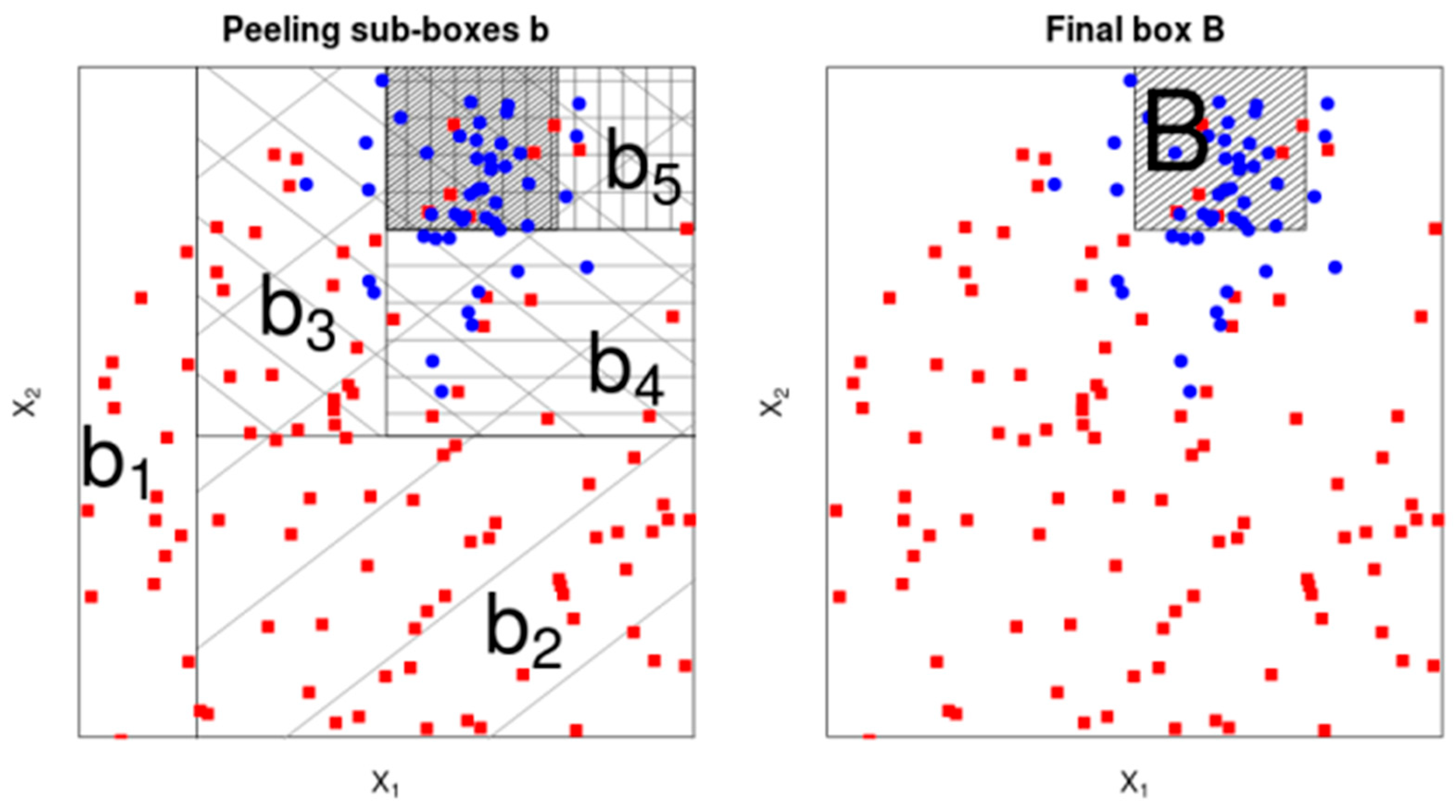
Figure 2.
The 5 steps in the R-PRIM framework for breast cancer classification.
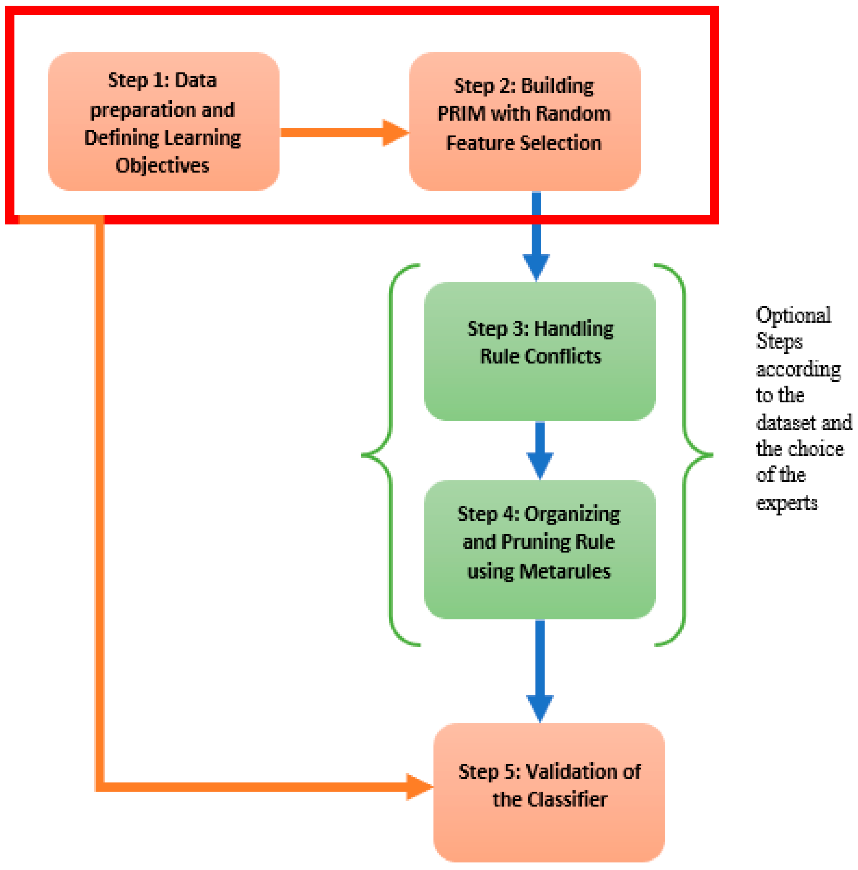
Figure 3.
An illustration of the overlapping between class labels and its different cases.
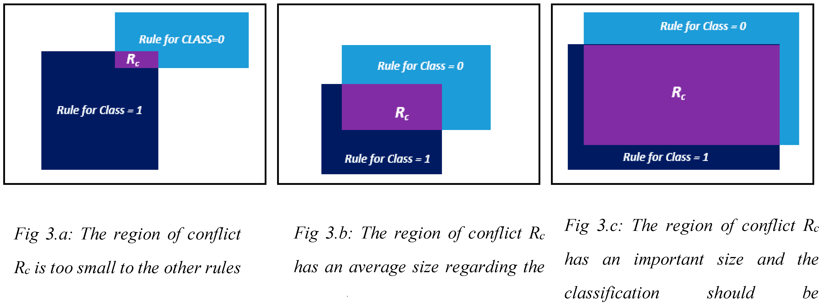
Figure 4.
An illustration of the organization of the rule space using Metarules.
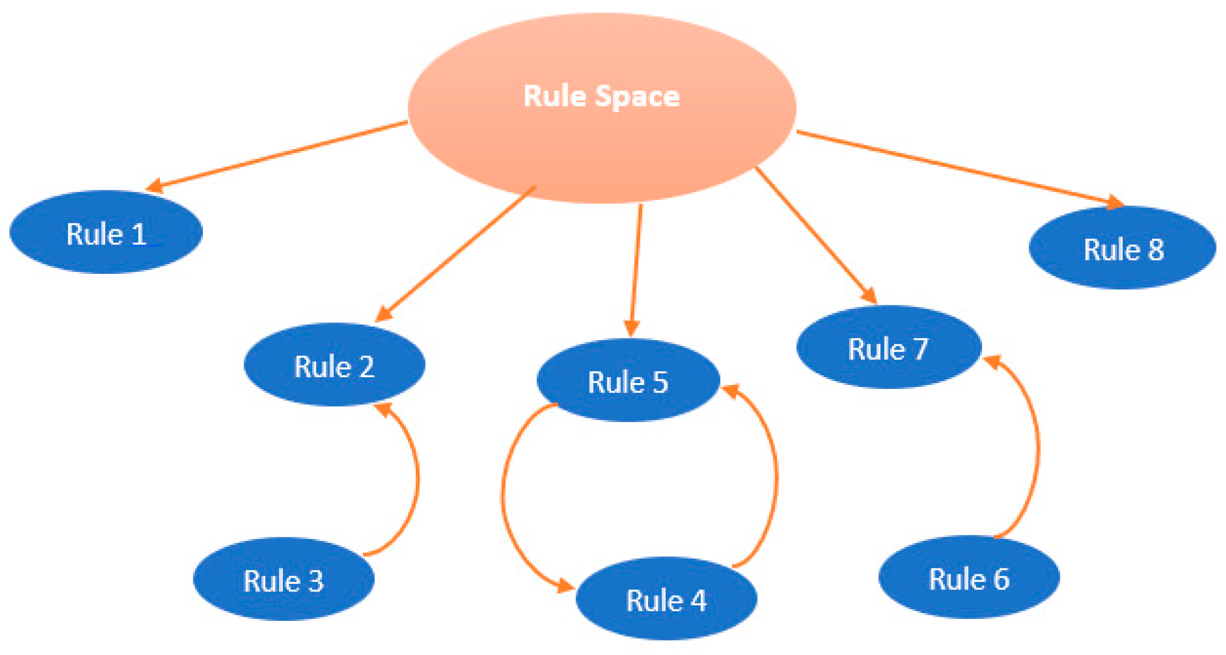
Figure 5.
Example of the construction of instance matrices. For every instance in the table, we put 1 if the instance is in the rule and 0 if it is not. So that for every class the matrix of instances is the entry for the association rule. Thus, we can find all the association between the rules and select the most important ones to reorganize our ruleset according to the confidence and support. Figure 5.a and Figure 5.b both show that the procedure is the same for both classes.
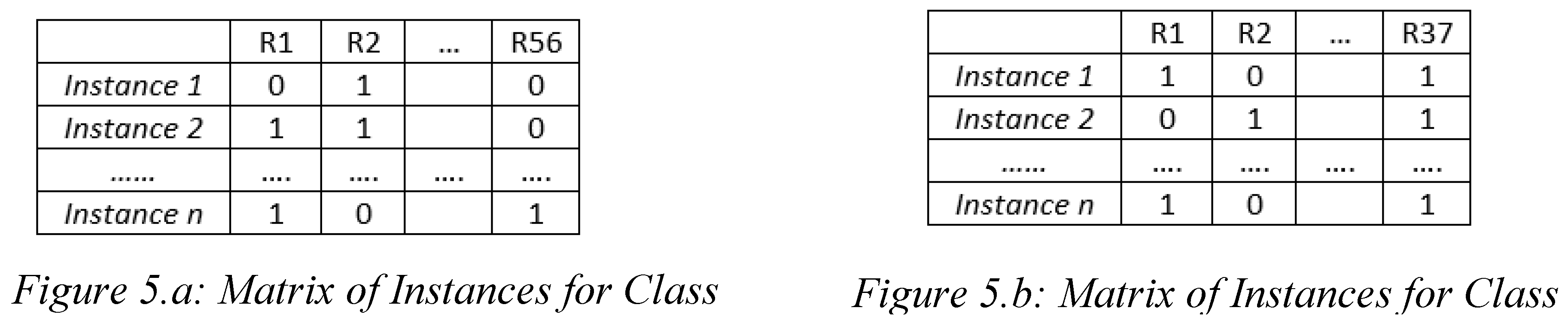
Figure 6.
The accuracy of the models for each dataset using Random Forest, Logistic Regression, XGBOOST and R-PRIM framework.
Figure 6.
The accuracy of the models for each dataset using Random Forest, Logistic Regression, XGBOOST and R-PRIM framework.
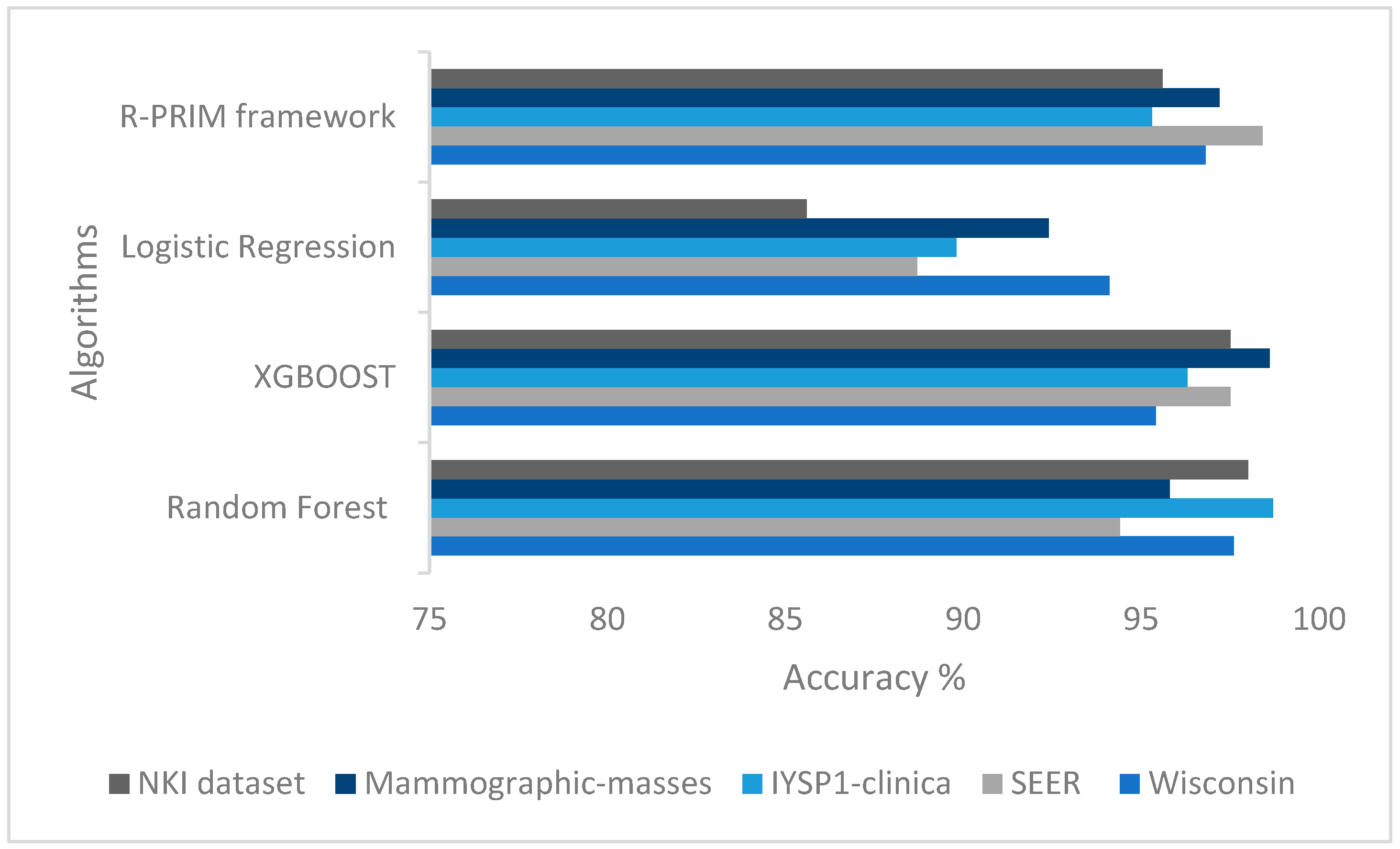

Table 1.
Rules constructed by the modified version of PRIM for “Class = 1” and “Class = 0” with their corresponding Coverage, Density, Support and the Dimension of each rule.
Table 1.
Rules constructed by the modified version of PRIM for “Class = 1” and “Class = 0” with their corresponding Coverage, Density, Support and the Dimension of each rule.
| Rules for class = 1 | Coverage | Density | Dimension | Support |
|---|---|---|---|---|
|
R1: 128.0 < Glucose < 199.0 AND 17.0 < SkinThickness < 99.0 AND 0.0 < Insulin < 520.0 AND 0.257 < DiabetesPedigreeFunction < 2.42 AND 25.0 < Age < 57.0 R2: 111.0 < Glucose < 199.0 AND 56.0 < BloodPressure < 122.0 AND 0.0 < SkinThickness < 43.0 AND 0.078 < DiabetesPedigreeFunction < 1.37 AND 32.0 < Age < 54.0 R3: 100.0 < Glucose < 199.0 AND 0.253 < DiabetesPedigreeFunction < 1.16 AND 29.0 < Age < 62.0 R4: 90.0 < Glucose < 199.0 AND 0.1495 < DiabetesPedigreeFunction < 2.42 AND 22.0 < Age < 81.0 R5: 0.0 < BloodPressure < 82.0 AND 12.0 < SkinThickness < 99.0 AND 0.0 < Insulin < 99.0 AND 0.1265 < DiabetesPedigreeFunction < 2.42 AND 24.0 < Age < 81.0 R6: 89.0 < Glucose < 199.0 AND 0.1265 < DiabetesPedigreeFunction < 2.42 R7: 128.0 < Glucose < 199.0 AND 17.0 < SkinThickness < 99.0 AND 25.0 < Age < 56.0 R8: 101.0 < Glucose < 199.0 AND 60.0 < BloodPressure < 85.0 AND 0.0 < SkinThickness < 26.0 AND 33.0 < Age < 52.0 R9: 109.0 < Glucose < 199.0 AND 12.0 < SkinThickness < 99.0 AND 31.0 < Age < 59.0 R10: 124.0 < Glucose < 199.0 AND 0.0 < SkinThickness < 0.0 AND 25.0 < Age < 53.0 R11: 95.0 < Glucose < 199.0 AND 22.0 < Age < 62.0 R12: 0.0 < BloodPressure < 85.0 AND 7.0 < SkinThickness < 99.0 AND 26.0 < Age < 56.0 R13: 93.0 < Glucose < 199.0 AND 60.0 < BloodPressure < 92.0 R14: 130.0 < Glucose < 199.0 AND 30.05 < BMI < 67.1 R15: 109.0 < Glucose < 199.0 AND 27.85 < BMI < 67.1 R16: 95.0 < Glucose < 199.0 AND 22.79 < BMI < 67.1 R17: 7.0 < Pregnancies < 9.0 AND 145.0 < Glucose < 199.0 AND 0.0 < Insulin < 495.0 R18: 128.0 < Glucose < 199.0 AND 18.0 < SkinThickness < 99.0 AND 74.0 < Insulin < 478.0 R19: 109.0 < Glucose < 199.0 R20: 7.0 < Pregnancies < 17.0 AND 84.0 < Glucose < 199.0 R21: 0.0 < Pregnancies < 3.0 AND 77.0 < Glucose < 199.0 AND 13.0 < SkinThickness < 45.0 AND 36.0 < Insulin < 846.0 R22: 4.0 < Pregnancies < 6.0 AND 0.0 < Glucose < 105.0 AND 0.0 < SkinThickness < 42.0 AND 0.0 < Insulin < 156.0 R23: 0.0 < Pregnancies < 2.0 AND 90.0 < Glucose < 199.0 AND 0.0 < SkinThickness < 42.0 AND 0.0 < Insulin < 15.0 R24: 8.0 < Pregnancies < 17.0 AND 24.0 < SkinThickness < 43.0 AND 31.0 < BMI < 45.90 R25: 30.05 < BMI < 67.1 R26: 7.0 < Pregnancies < 17.0 AND 0.0 < BloodPressure < 94.0 AND 23.15 < BMI < 67.1 R27: 4.0 < Pregnancies < 17.0 AND 0.0 < BloodPressure < 80.0 AND 0.0 < SkinThickness < 24.0 R28: 3.0 < Pregnancies < 17.0 AND 0.0 < SkinThickness < 33.0 R29: 0.0 < BloodPressure < 86.0 AND 23.15 < BMI < 29.5 R30: 28.1 < BMI < 67.1 AND 0.20 < DiabetesPedigreeFunction < 2.42 AND 31.0 < Age < 60.0 R31: 29.0 < Insulin < 846.0 AND 26.1 < BMI < 67.1 AND 0.1275 < DiabetesPedigreeFunction < 2.42 AND 28.0 < Age < 53.0 R32: 26.9 < BMI < 67.1 AND 0.1265 < DiabetesPedigreeFunction < 2.42 AND 25.0 < Age < 62.0 R33: 0.0 < Insulin < 194.0 AND 22.79 < BMI < 67.1 AND 0.1195 < DiabetesPedigreeFunction < 0.817 AND 23.0 < Age < 81.0 R34: 22.0 < Age < 54.0 R35: 24.75 < BMI < 67.1 R36: 30.85 < BMI < 67.1 R37: 23.25 < BMI < 67.1 R38: 0.0 < BMI < 23.05 R39: 7.0 < Pregnancies < 12.0 AND 110.0 < Insulin < 846.0 AND 0.188 < DiabetesPedigreeFunction < 2.42 R40: 0.3235 < DiabetesPedigreeFunction < 2.42 R41: 7.0 < Pregnancies < 12.0 AND 64.0 < BloodPressure < 122.0 AND 0.1215 < DiabetesPedigreeFunction < 0.2825 R42: 0.11 < DiabetesPedigreeFunction < 0.2825 R43: 0.0 < Insulin < 140.0 AND 0.086 < DiabetesPedigreeFunction < 2.42 R44: 7.0 < Pregnancies < 9.0 AND 145.0 < Glucose < 199.0 AND 0.0 < Insulin < 495.0 R45: 134.0 < Glucose < 199.0 AND 0.0 < Insulin < 478.0 R46: 109.0 < Glucose < 199.0 R47: 7.0 < Pregnancies < 17.0 AND 84.0 < Glucose < 199.0 R48: 0.0 < Pregnancies < 3.0 AND 78.0 < Glucose < 199.0 AND 36.0 < Insulin < 846.0 R49: 4.0 < Pregnancies < 6.0 AND 0.0 < Glucose < 104.0 AND 0.0 < Insulin < 156.0 R50: 0.0 < Pregnancies < 2.0 AND 90.0 < Glucose < 199.0 AND 0.0 < Insulin < 15.0 R51: 28.1 < BMI < 67.1 AND 0.20 < DiabetesPedigreeFunction < 2.42 AND 31.0 < Age < 60.0 R52: 26.70 < BMI < 35.45 AND 0.1275 < DiabetesPedigreeFunction < 2.42 AND 30.0 < Age < 53.0 R53: 29.95 < BMI < 67.1 AND 0.1265 < DiabetesPedigreeFunction < 2.42 AND 25.0 < Age < 81.0 R54: 23.35 < BMI < 67.1 AND 0.1275 < DiabetesPedigreeFunction < 0.6535 AND 28.0 < Age < 61.0 R55:0.1195 < DiabetesPedigreeFunction < 2.42 AND 22.0 < Age < 60.0 R56: 27.85 < BMI < 67.1 AND 21.0 < Age < 62.0 |
0.29 0.24 0.16 0.24 0.02 0.03 0.34 0.14 0.08 0.11 0.23 0.03 0.03 0.51 0.26 0.18 0.14 0.22 0.48 0.06 0.04 0.02 0.01 0.11 0.69 0.08 0.06 0.03 0.03 0.5 0.1 0.21 0.11 0.059 0.018 0.74 0.24 0.01 0.12 0.56 0.067 0.20 0.03 0.14 0.40 0.31 0.05 0.04 0.02 0.01 0.5 0.09 0.21 0.05 0.12 0.02 |
0.77 0.63 0.52 0.22 0.15 0.13 0.75 0.63 0.53 0.71 0.22 0.25 0.16 0.73 0.39 0.22 0.88 0.64 0.39 0.4 0.12 0.14 0.09 0.75 0.43 0.45 0.27 0.14 0.09 0.62 0.49 0.36 0.22 0.11 0.11 0.46 0.24 0.04 0.82 0.37 0.43 0.25 0.16 0.88 0.59 0.34 0.4 0.11 0.14 0.09 0.62 0.53 0.38 0.32 0.14 0.17 |
5 5 3 3 5 2 3 4 3 3 2 3 2 2 2 2 3 3 1 2 4 4 4 3 1 3 3 2 2 3 4 3 4 1 1 1 1 1 3 1 3 1 2 3 2 1 2 3 3 3 3 3 3 3 2 2 |
0.13 0.13 0.10 0.38 0.05 0.08 0.16 0.08 0.05 0.05 0.37 0.05 0.08 0.24 0.22 0.28 0.05 0.12 0.42 0.05 0.12 0.06 0.05 0.05 0.55 0.05 0.07 0.07 0.12 0.27 0.07 0.20 0.17 0.18 0.05 0.56 0.34 0.08 0.05 0.52 0.05 0.27 0.07 0.06 0.23 0.31 0.05 0.13 0.06 0.05 0.27 0.06 0.18 0.05 0.29 0.05 |
| Rules for class = 0 | ||||
|
R1: 94.0 < Glucose < 157.0 AND 0.0 < BloodPressure < 88.0 AND 60.0 < Insulin < 228.0 AND 0.078 < DiabetesPedigreeFunction < 0.899 AND 21.0 < Age < 49.0 R2: 89.0 < Glucose < 183.0 AND 0.0 < BloodPressure < 90.0 AND 0.0 < SkinThickness < 41.0 AND 0.0 < Insulin < 190.0 AND 0.078 < DiabetesPedigreeFunction < 1.1855 AND 21.0 < Age < 59.0 R3: 80.0 < Glucose < 189.0 AND 52.0 < BloodPressure < 82.0 AND 12.0 < SkinThickness < 39.0 AND 49.0 < Insulin < 394.0 AND 0.259 < DiabetesPedigreeFunction < 2.42 R4: 70.0 < BloodPressure < 106.0 AND 16.0 < SkinThickness < 50.0 AND 0.0 < Insulin < 145.0 AND 0.1535 < DiabetesPedigreeFunction < 0.712 R5: 52.0 < BloodPressure < 122.0 AND 0.0 < Insulin < 485.0 AND 0.239 < DiabetesPedigreeFunction < 2.42 R6: 0.0 < Glucose < 189.0 AND 0.11 < DiabetesPedigreeFunction < 1.143 R7: 93.0 < Glucose < 137.0 AND 54.0 < BloodPressure < 88.0 AND 7.0 < SkinThickness < 40.0 AND 21.0 < Age < 52.0 R8: 90.0 < Glucose < 157.0 AND 23.25 < BMI < 41.65 R9: 19.20 < BMI < 47.34 R10: 0.0 < Pregnancies < 0.0 AND 13.0 < SkinThickness < 45.0 AND 63.0 < Insulin < 291.0 R11: 2.0 < Pregnancies < 7.0 AND 92.0 < Glucose < 133.0 AND 0.0 < SkinThickness < 39.0 AND 73.0 < Insulin < 267.0 R12: 1.0 < Pregnancies < 8.0 AND 105.0 < Glucose < 169.0 AND 0.0 < SkinThickness < 47.0 AND 74.0 < Insulin < 846.0 R13: 1.0 < Pregnancies < 17.0 AND 80.0 < Glucose < 199.0 AND 0.0 < SkinThickness < 41.0 AND 0.0 < Insulin < 220.0 R14: 56.0 < Glucose < 199.0 AND 0.0 < SkinThickness < 51.0 AND 0.0 < Insulin < 474.0 R15: 0.0 < BloodPressure < 88.0 AND 21.45 < BMI < 43.55 R16: 0.0 < Pregnancies < 10.0 AND 17.0 < SkinThickness < 46.0 AND 20.6 < BMI < 46.15 R17: 0.0 < BloodPressure < 94.0 AND 0.0 < SkinThickness < 47.0 AND 0.0 < BMI < 51.15 R18: 40.0 < Insulin < 215.0 AND 25.1 < BMI < 41.65 AND 0.078 < DiabetesPedigreeFunction < 1.18 AND 21.0 < Age < 46.0 R19: 20.6 < BMI < 43.34 AND 0.078 < DiabetesPedigreeFunction < 0.9155 R20: 15.0 < Insulin < 846.0 AND 0.0 < BMI < 46.6 AND 0.247 < DiabetesPedigreeFunction < 2.2125000000000004 R21: 0.0 < Insulin < 14.0 R22: 0.0 < BloodPressure < 88.0 AND 21.45 < BMI < 43.55 R23: 0.0 < BloodPressure < 106.0 AND 19.20 < BMI < 46.150 R24: 0.0 < BloodPressure < 108.0 R25: 0.0 < Pregnancies < 1.0 AND 62.0 < BloodPressure < 84.0 AND 60.0 < Insulin < 265.0 R26: 2.0 < Pregnancies < 7.0 AND 70.0 < BloodPressure < 88.0 AND 56.0 < Insulin < 160.0 AND 0.078 < DiabetesPedigreeFunction < 0.69 R27: 0.0 < BloodPressure < 90.0 AND 0.0 < Insulin < 220.0 AND 0.1405 < DiabetesPedigreeFunction < 1.1855 R28: 0.0 < Pregnancies < 3.0 AND 52.0 < BloodPressure < 106.0 AND 14.0 < Insulin < 540.0 AND 0.094 < DiabetesPedigreeFunction < 2.42 R29: 1.0 < Pregnancies < 17.0 AND 64.0 < BloodPressure < 108.0 AND 0.098 < DiabetesPedigreeFunction < 2.42 R30: 0.0 < Pregnancies < 2.0 AND 65.0 < Insulin < 291.0 R31: 0.0 < Pregnancies < 10.0 AND 89.0 < Glucose < 169.0 AND 56.0 < Insulin < 846.0 R32: 1.0 < Pregnancies < 17.0 AND 75.0 < Glucose < 199.0 AND 0.0 < Insulin < 0.0 R33: 0.0 < Pregnancies < 6.0 AND 56.0 < Glucose < 187.0 R34: 0.0 < Glucose < 195.0 R35: 23.25 < BMI < 42.5 AND 0.078 < DiabetesPedigreeFunction < 1.09AND 21.0 < Age < 58.0 R36: 19.45 < BMI < 49.65AND 0.2355 < DiabetesPedigreeFunction < 1.31 R37: 0.10 < DiabetesPedigreeFunction < 2.42 AND 22.0 < Age < 81.0 |
0.25 0.42 0.07 0.06 0.14 0.05 0.32 0.61 0.36 0.07 0.10 0.14 0.51 0.15 0.84 0.06 0.08 0.31 0.55 0.06 0.07 0.84 0.11 0.04 0.12 0.07 0.64 0.06 0.08 0.24 0.18 0.38 0.16 0.04 0.77 0.16 0.07 |
0.76 0.66 0.84 0.71 0.54 0.43 0.71 0.68 0.62 0.86 0.79 0.70 0.63 0.57 0.66 0.78 0.57 0.75 0.63 0.67 0.56 0.66 0.66 0.54 0.85 0.81 0.64 0.78 0.57 0.78 0.66 0.63 0.61 0.48 0.67 0.67 0.49 |
5 6 5 4 3 2 4 2 1 3 4 4 4 3 2 3 3 4 2 3 1 2 2 1 3 4 3 4 3 2 3 3 2 1 3 2 2 |
0.22 0.42 0.06 0.06 0.16 0.07 0.30 0.58 0.37 0.05 0.09 0.13 0.53 0.17 0.83 0.05 0.09 0.27 0.56 0.06 0.08 0.83 0.11 0.05 0.09 0.05 0.65 0.05 0.10 0.20 0.18 0.40 0.17 0.06 0.74 0.16 0.09 |
Table 2.
Major properties of the datasets considered in the evaluation.
| Datasets | Nb of instances | Nb of attributes | Class labels | Class distribution |
| Wisconsin SEER ISPY1-clinica Mammographic-masses NKI dataset |
569 4024 168 961 272 |
32 12 18 6 1570 |
Malignant : 1 Benign: 0 Alive: 0 Dead: 1 No: not dead :0 Yes: dead: 1 1: malignant 0: benign 1: dead 0: alive |
359 210 3408 616 32 136 445 516 195 77 |
Table 3.
Number of rules generated by the framework before and after the Metarules’ step.
| Number of rules per class | ||||
|---|---|---|---|---|
| Before the Metarules | After the Metarules | |||
| 0 | 1 | |||
| Wisconsin SEER IYSP1-clinica Mammographic-masses NKI dataset |
36 28 5 14 38 |
45 72 12 12 54 |
19 15 5 9 12 |
34 44 11 9 33 |
Table 4.
Empirical Results of 5 real-life breast cancer datasets using Random Forest (RF), XGBoost (XGB), Logistic Regression (LR) and PRIM based classifier framework and the measures of their models.
Table 4.
Empirical Results of 5 real-life breast cancer datasets using Random Forest (RF), XGBoost (XGB), Logistic Regression (LR) and PRIM based classifier framework and the measures of their models.
| ACCURACY | PRECISION | RECALL | F1-SCORE | |||||||||||||
|---|---|---|---|---|---|---|---|---|---|---|---|---|---|---|---|---|
| RF | XG | LR | PRIM based classifier | RF | XGB | LR | PRIM based classifier | RF | XGB | LR | PRIM based classifier | RF | XGB | LR | PRIM based classifier | |
| Wisconsin SEER IYSP1-clinica Mammographic-masses NKI dataset |
97.6 94.4 98.7 95.8 98 |
95.4 97.5 96.3 98.6 97.5 |
94.1 88.7 89.8 92.4 85.6 |
96.8 98.4 95.3 97.2 95.6 |
98.2 95.6 98.9 97.7 97.9 |
98 97.6 95.2 96.3 94.5 |
94.8 88.1 86.5 92.4 93.3 |
95.6 97.1 94.6 96.3 96.7 |
93.9 98 97.2 97.5 97.8 |
96.7 97.2 95.4 98.7 96.7 |
85.4 86.7 89.9 93.2 94.1 |
94.2 95.6 94.8 95.8 97.1 |
96 | 97.3 | 89.9 | 94.9 96.3 94.7 96.1 96.9 |
| 96. 7 | 97.3 | 87.4 | ||||||||||||||
| 98 | 95.3 | 88.2 | ||||||||||||||
| 97. 6 | 97.4 | 92.8 | ||||||||||||||
| 97. 8 | 95.6 | 93.7 | ||||||||||||||
Disclaimer/Publisher’s Note: The statements, opinions and data contained in all publications are solely those of the individual author(s) and contributor(s) and not of MDPI and/or the editor(s). MDPI and/or the editor(s) disclaim responsibility for any injury to people or property resulting from any ideas, methods, instructions or products referred to in the content. |
© 2024 by the authors. Licensee MDPI, Basel, Switzerland. This article is an open access article distributed under the terms and conditions of the Creative Commons Attribution (CC BY) license (http://creativecommons.org/licenses/by/4.0/).
Copyright: This open access article is published under a Creative Commons CC BY 4.0 license, which permit the free download, distribution, and reuse, provided that the author and preprint are cited in any reuse.


