
Submitted:
11 December 2024
Posted:
12 December 2024
You are already at the latest version
Abstract
The air we breathe consists of contaminants such as particulate matter (PM), carbon dioxide (CO2), nitrogen dioxide (NO2), nitric oxide (NO) which when inhaled brings about several changes in the autonomous responses of our body. Our previous work showed that we can use the human body as a sensor by making use of autonomous responses (or biometrics) such as changes in electrical activity in the brain measured using electroencephalogram (EEG) and physiological changes such as skin temperature, Galvanic Skin Response (GSR), blood oxygen saturation (SpO2) and few others can be used to estimate pollutants, in particular, PM1 and CO2 with high degree of accuracy using machine learning. In this study, we introduce a novel approach to obtain the power spectral density (PSD) from the timeseries of EEG developed by Astrapi called the Astrapi Spectrum Analyzer (ASA). The physiological responses of a participant cycling outdoors is measured using a biometric suite and ambient CO2, NO2 and NO is measured simultaneously. We made use of physiological responses and combined it with the PSD from an EEG timeseries using Welch Method (WM) and then with the PSD using ASA to estimate the inhaled concentration of CO2, NO2 and NO. This work shows that, indeed the PSD obtained from ASA combined with other physiological responses provides much better result (RMSE=9.28 ppm in an independent test set) in estimating inhaled CO2 compared to making use of the same physiological responses and PSD from WM (RMSE=17.55 ppm in an independent test set). Small improvements are also seen in the estimation of NO2 and NO when using physiological responses and PSD from ASA, which can be further confirmed by making use of large number of data collection.
Keywords:
Power Spectral Density
; Astrapi Spectrum Analyzer
; biometrics
; physiological responses
1. Introduction
Several factors affect human health, among which air pollution is one of the major concerns in the present world. As shown by data from the World Health Organization, 7 million premature deaths are associated with the combination of outdoor and indoor pollution and millions of people fall ill by breathing polluted air [1]. The United States Environmental Protection Agency (USEPA) establishes National Ambient Air Quality Standards (NAAQS) for 6 pollutants, including carbon monoxide (CO), particulate matter (PM), nitrogen dioxide (), lead (Pb), ozone () and sulfur dioxide () [2]. These principal components also known as criteria pollutants are considered harmful not just to people’s health but also to the environment. In addition to the pollutants mentioned above, exposure to other pollutants such as carbon dioxide (), nitrogen oxide (NO), and black carbon also causes several health problems. The sources of these pollutants in microenvironments can be from cooking, emissions from vehicle and industry, smoking, construction sites, poor indoor ventilation, while large scale air pollution can be caused by wildfires, volcanic eruptions.
Exposure to with a 1-hour moving average ranging from 350 parts per million (ppm) to 3,300 ppm has been found to deteriorate cognitive performance in children [3], cognitive function among participants was also found to decrease when levels increased 600 ppm to 1,000 ppm and 2,500 ppm in 3 different 2.5 hour sessions [4]. Physiological parameters such as cardiovasular function have been known to be affected when average concentration is at 2,000 ppm [5]. Studies have also shown that heart rate and blood pressure were affected when concentration was increased from 500 ppm to 3000 ppm [6]. The NAAQS set by the EPA for nitrogen oxides, which includes are: a standard level for 1 hour of 100 parts per billion (ppb) and an annual standard level of 53 ppb. Exposure to indoor has been associated with aggravating respiratory symptoms in children [7,8]. Although limited studies have been conducted on short-term exposure to , long-term exposure has been associated with cardiovascular problems, respiratory symptoms, and hospital admissions [9,10]. Limited studies have also been conducted on the short-term effects of NO inhalation. Although regulated NO is used in medications, a higher concentration is considered toxic [11]. Inhaled NO can also interact with oxygen in the lungs to form which is a potential pulmonary irritant [12,13].
Since higher concentrations of pollutants are also dealt with in our daily life in microenvironments for a short period of time, our previous work studied the effects of PM [14] and gases [15] such as , and NO in the human body in small temporal (∼5 secs) and spatial scales (∼ 1 meter). More importantly, these two studies showed that, from a series of cognitive and physiological changes brought in the human body by pollutants, we can indeed make use of a set of responses such as measurement of electrical activities in the brain using electroencephalogram (EEG), measurement of electrical activity in the heart using electrocardiogram (ECG), skin temperature, heart rate variability, heart rate, respiration rate, blood oxygen saturation (), galvanic skin response (GSR), pupil diameter, distance between pupils to accurately predict the inhaled concentration of and with a very high accuracy as indicated by the coefficient of determination () of 0.99 and 0.91 respectively between the true and estimated values of these pollutants using machine learning regression. In these two studies, the measured voltage time series from the 64-electrode EEG device was transformed into a powerspectrum using the Welch method (WM) [16]. The powerspectrum along with other physiological changes as mentioned above, served as input variables in a machine learning model to estimate the inhaled concentration of PM, , and NO. The use of machine learning has been very useful in studying several environmental factors such as characterizing water composition [17], remote sensing [18], estimating global PM for human health [19].
In this study, we use a new algorithm developed by Astrapi (https://www.astrapi-corp.com/, accessed on 14 November 2024) to transform the voltage time series obtained from EEG into a powerspectrum. The Astrapi Spectrum Analyzer (ASA) uses a new application of the superheterodyne principle of telecommunications to shift spectral data to lower frequencies where it is easier to digitally filter and measure the power in each frequency range. This approach avoids the implicit assumption that the spectrum is at least approximately stationary (constant power in each frequency), which is the underlying priori knowledge for Fourier transform (FT)-based algorithms. Since in practice spectra are never stationary, techniques such as windows and wavelets have been layered on top of the FT to "stitch together" time intervals over which the spectrum is expected to be approximately stationary (as with, for instance, the Welch and Bartlett Methods). However, these techniques cannot deal correctly with a continuously non-stationary spectrum, the interval of approximate stationarity (if it exists) is generally not known in advance, and the extra operations required by these techniques introduce noise and delays. Consequently, the ASA is able to more accurately and efficiently measure spectral power in cases where the spectral data are highly nonstationary, as for the study reported here. Further details of the spectrum analyzer can be obtained from the following patents [20,21].
The main objective of this study is to make use of physiological responses such as average pupil diameter, pupil distance, ECG, respiration rate, , heart rate, GSR, skin temperature, and time series of electrical activity in the brain using a biometric suite which were captured when a participant was cycling outdoors wearing a biometric suite. These biometrics (or autonomous responses or input variables or physiological and cognitive responses or biological measurements) were then used to estimate the inhaled concentration of , and NO when a participant was cycling outdoors in two ways: (a) the input feature to a machine learning model are physiological responses and PSD obtained from ASA, (b) the input feature to a machine learning model are the same physiological responses as used before and the PSD obtained from WM. By doing so, we test which combination of power spectrum with the physiological responses is better for estimating the inhaled concentration of the 3 pollutants.
2. Materials and Methods
The methodology used in this study involves three key components which include: (a) simultaneously measuring biological measurements of a person cycling outdoors using a biometric suite and also measuring corresponding ambient , and NO; (b) among the series of biological measurements, convert the EEG data from timeseries of voltage to a power spectrum using WM and ASA (c) use the physiological responses and combine with the PSD obtained first from WM and then with PSD from ASA to estimate the inhaled concentration of , and NO separately using machine learning to test which combination of power spectrum and physiological responses does a better task of estimating inhaled concentration of the pollutants.
The data that has been used is from our previous study [14]. A brief description of the procedure of data collection is given below in Section 2.1 and Section 2.2.
2.1. Experimental Paradigm
Figure 1a shows the experimental paradigm of data collection in which a participant wearing a biometric suite is cycling outdoors. The biometric variables that were measured include EEG, ECG, , heart rate, respiration rate, GSR, skin temperature, pupil diameter of the left eye, pupil diameter of the right eye and 3 dimensional distance between the pupils. In order to reduce the number of dimensions, the average pupil diameter was calculated using the pupil diameter of each eye. An electric car is following behind consisting of sensors in the trunk to measure ambient , , NO and PM. The variation of these pollutants was entirely based on natural variation and no artificial source was used.
The EEG time series data was collected using the Cognionics headset (https://www.cgxsystems.com/, accessed on 18 November 2024), as shown in the bottom of Figure 1b. The headset consists of 64 electrodes following the 10–10 nomenclature system [22] with measurement at a sampling rate of 500 Hz. The time series of EEG from each of the 64 electrodes was then transformed to a PSD consisting of 5 bands: delta (1-3 Hz), theta(4-7 Hz), alpha (8-12 Hz), beta (13-25 Hz), and gamma (25-70 Hz), first by using the WM and then using the ASA. With the time series of 64 electrodes and each of the time series divided into 5 bands, a total of 320 biometric variables were used from the EEG headset alone.
Physiological responses such as ECG, GSR, , respiration rate, skin temperature, and heart rate were measured using a Cognionics AIM Generation 2 device (https://www.cgxsystems.com/auxiliary-input-module-gen2, accessed on 18 November 2024) as shown in Figure 1b, which were measured at a sampling rate of 500 Hz. The Tobii Pro Glasses 2 (https://www.tobii.com/products/discontinued/tobii-pro-glasses-2, accessed on 18 November 2024) is shown in Figure 1d. Although these eye tracking glasses provide several measurements, the ones that were considered are the pupil diameter of the left eye, the pupil diameter of the right eye, and the distance between the pupils which were measured at a sampling rate of 100 Hz.
The measurement of ambient was performed using the LI-COR LI-850 device (https://www.licor.com/env/support/LI-850/topics/description.htmlOnlineresources, accessed 18 November 2024). The device is shown at the top of Figure 1 c and the measurement was made at a sampling rate of 0.5 Hz (twice every second). The measurement device for and NO is shown at the bottom of Figure 1c and was carried out using the Model 405 nm /NO/ Monitor from 2B technologies (https://2btech.io/items/other-monitors/model-405-nm-no2-no-nox-monitor/, accessed 19 November 2024) at a sampling rate of 0.2 Hz (once every 5 s).
A summary of the list of biometric variables measured and the corresponding units is shown in Table 1
With the 320 biometric variables obtained from EEG and other variables such as ECG, GSR, , respiration rate, skin temperature, heart rate, average pupil diameter and distance between the pupils, gave a total of 328 biometric variables that have been considered in this study.
2.2. Data Collection
The process of data collection was carried out on a single participant because of the constraints from COVID-19. Data collection was carried out on 3 separate days in 2021 which include: May 26, June 9 and June 10 in Breckenridge Park, Richardson, TX. A map of the location of bike ride and the track used is shown in Figure 2, which was recorded using a Global Positioning System (GPS) that was placed on the bike.
Data collection started on the first track on a day as indicated by the red asterisk in Figure 2a. Data collection on the first track was stopped for a while at the location as indicated by the black asterisk in Figure 2a before the data collection was started on second track as shown by the black asterisk sign in Figure 2b. Multiple loops were taken in the second track before the data collection was stopped. These two tracks were used on multiple days for data collection.
Table 2 shows a summary of data collection of the three pollutants:
2.3. Machine Learning Model Development
The estimation of inhaled , and NO was done in two different ways: (a) first, by using the physiological responses and EEG power spectrum obtained from WM as input variables; (b) second, by using the same physiological responses and power spectrum obtained from ASA as input variables to the random forest algorithm [23] for non-linear, multidimensional data with hyperparameter optimization which was implemented using scikit-learn (version 1.5.1) [24] in Python 3.12.4. 80% of the data set was used for training the model whereas 20% of the dataset was used as an independent test set. The accuracy of the prediction was quantified by calculating the root mean square error (RMSE) and coefficient of determination () between the true and estimated values whereas qualitative assessment was done by plotting Quantile-Quantile plot and a scatter plot.
Since, a large number of biometric variables were used for the estimation, in order to identify the effectiveness of biometric variables in the process of estimation, a bar plot of SHAP values (SHapley Additive exPlanations) [25,26] from the SHAP library (version 0.46.0) have been used to rank the input variables based on their importance for prediction in a descending order.
3. Results
Each of the pollutants, , and NO that have been estimated in this study have a total of 328 biometric variables as input features whereas a small number of data records are available for each of them as shown in Table 2. Since a large number of dimension have been used and a relatively small number of data records is available, the metrics that have been used to assess the goodness of fit can change based on the how the data is shuffled. As a result, the machine learning model was ran a total of 100 times, and the RMSE and values between the true and estimated values of the pollutants in an independent set have been recorded and the average of these numbers have also been calculated. The hyperparameters that were optimized and those that were used in the machine learning model is given in Table A1 and Table A2 in Appendix A.
Table 3 shows the average and average RMSE between the true and estimated values in an independent test set when the machine learning model was ran a total of 100 times. The input features have the same physiological responses, while the PSD is either from WM or ASA.
Table 3 shows, that there is significant improvement in the RMSE value in an independent test set of when the input feature were a combination of physiological responses and PSD from ASA, while the results for average test RMSE and average test provide small improvements in the case of and NO.
Figure 3a shows changes in RMSE in an independent test for in each of the trials when the physiological responses was first combined with PSD from WM and then with PSD from ASA. The figure shows that, apart from a couple of cases, for most part of the trial, the RMSE was smaller when PSD from ASA was used with other biometrics. On the other hand, Figure 3b shows that the results of test RMSE in the case of and NO have a small improvement.
Similarly, Figure 4 shows the line graph of the value between the true and estimated values of the pollutant in an independent test set in each of the 100 trial. Figure 4a shows that, in the case of , the value is closer to 1 for most of the occasions when physiological responses was combined with PSD from ASA when compared to the PSD from WM. Similarly, small improvement in test can be seen in the case of and NO as well which is shown in Figure 4a and Figure 4b respectively.
Scatter plot of an instance among the 100 trials for each of the pollutant is shown in Figure 5. On the left we have the scatter diagram when the input feature was a combination of physiological responses and PSD from ASA, whereas on the right in the input feature was a combination of physiological responses and PSD from WM. As there are improvement in the estimation when PSD from ASA was used, a lot of points on the scatter on the left are closer to the 1:1 line than the one on the right. This is clearly visible, for as significant improvement was obtained in this case as compared to the case of and NO.
An instance of Quantile-Quantile plot among the 100 trials is shown in Figure 6. On the left, the Quantile-Quantile plot in the train and in the test set is shown when the physiological responses were combined with PSD from ASA whereas on the right the plots show the Quantile-Quantile plot when the physiological responses was combined with PSD from WM. It can be seen, that in Figure 6a, the quantiles are closer to the 1:1 line for most of the distribution in both the training and the testing set as compared to Figure 6b. For the case of and NO, the Quantile-Quantile plots indicate that the distribution is closer to the 1:1 line for smaller values of the pollutants.
In the process of estimating inhaled concentration of , and NO, we have used a large number of input variables, in particular 328. As mentioned in Section 2.3, in order to identify the importance of features, SHAP value summary plot is plotted which is shown in Figure 7. The bar graphs are arranged in descending order such that feature with the highest importance is at the top. Since, the input features are high, the ranking of the variables, especially when the SHAP values are close, can change when the data is shuffled whereas the ranking of the variables at the top remain to be consistent as the SHAP values are higher compared to other variables. Figure 7 a, c and e are feature importance plots when physiological response was combined with PSD from ASA whereas figures on the right, Figure 7 b, d and f are feature importance plots when the same physiological responses was combined with PSD from WM. Each of the feature importance plots shows that, responses such as average pupil diameter, GSR, skin temperature, respiration rate and ECG are common in most of cases.
Few of the EEG electrode and their corresponding band also seems to appear in some cases. The electrodes with even and those with odd numbers after the letters are located on the right side and left side of the brain respectively [22]. The FT electrode variable, as shown in Figure 7a and c is located between the frontal and temporal lobe, the T7 electrode variable, as shown in Figure 7b is located on the temporal lobe on the left side of the brain whereas the P8 electrode variable, as shown in Figure 7e is located in the parietal lobe on the right side of the brain.
4. Discussion
The human body responds to a lot of factors such as temperature, altitude, humidity, air quality, external light, and several other environmental variables. The underlying principle that we used in this study and the one we performed before [14,15] used autonomous responses (or biometrics) in the human body that resulted from the intake of pollutants in the air. Our results show that these autonomous responses can be used to estimate the inhaled concentration of inhaled and PM [14] with high precision using machine learning regression. The basis of all these studies is to use the body as a sensor.
The main contribution of this study is the introduction of Astropi Spectrum Analyzer (ASA), which is a novel approach to convert the time series of electrical activities in the brain measured using EEG to a power spectrum density of various bands. We used physiological responses and PSD from ASA as well as PSD from WM to estimate the inhaled concentration of , and NO. The results shown in Table 2, show that when physiological responses are combined with PSD from ASA, provide significant improvements in the estimation of as indicated by average RMSE in a test set of 9.28 ppm compared to the estimation made using the same physiological responses and PSD from WM as indicated by average RMSE in an independent test of 17.55 ppm when the machine learning model was run 100 times. These improvements can also be seen by comparing the scatter diagram in Figure 5a and Figure 5b and also by comparing the Quantile-Quantile plot in Figure 6a and Figure 6b, where the values are closer to their corresponding 1:1 line when the input variables considered were a combination of physiological responses and PSD from ASA rather than when combined with PSD from WM.
However, the improvements in the results of the estimation of inhaled and NO were found to be small. One possible reason for the small improvement could be the PSD from EEG that has small SHAP values or small contribution to the estimation of and NO. This is shown in Figure 7c and Figure 7e which shows the shap summary plot for and NO respectively. Each of these figure shows that there only is a single feature from the EEG PSD among the top 9 features that contributed the most in estimating these pollutants. As the contribution of EEG PSD for these pollutants is small, the improvements in the result was also small.
The results for the estimation of and NO is also not as highly accurate as compared to the case of and PM. As we hypothesized previously [14,15], the autonomous responses was most likely dominated by the inhalation of PM and , because of which the estimation of these two pollutants was found to be high when compared to the estimation of and NO. The results for and NO however are accurate for their smaller values as indicated by the scatter diagram in Figure 5c, d, e and f and the Quantile-Quantile plot in in Figure 6c, d, e and f. We do predict that the collection of large numbers of data for these two pollutants can improve the accuracy in the prediction of these two pollutants so that the machine learning model can learn from training data over a wide range of data and then be tested in an independent test set. This can also be seen in the same scatter diagram and the Quantile-Quantile plot, where the data points deviate from their corresponding 1:1 line as the data points become scarce for higher values of their pollutants.
The study has two key limitations. First, the limited set of data. This limitation can be removed by collection of large number of data which can be achieved by increasing the time of data collection. Second, the the use of a single participant limits the generalizability of the findings. While multiple trials were conducted at different location for data collection, future study can include multiple participants over a wide range of demographics to enhance the generalizability.
It should be noted that improvements in the estimation of inhaled concentration of was achieved despite the fact that only a few features of EEG PSD obtained using ASA contributed the most to the estimation of the pollutant, as shown in Figure 7a. It is reasonable to expect that the relative advantage of ASA will be even greater for applications that are more purely based on spectral data, a topic for future research.
Author Contributions
Conceptualization, D.L., S.R., J.P., T.B., and S.T. ; methodology, D.L., S.R., J.P., T.B., S.T., T.L.; software, S.R., S.T., J.P., T.B., A.F.; formal analysis, S.R., D.L., T.B., J.P.; data curation, S.T., D.L., A.F., L.W., J.W., P.D., T.L., M.L., A.A.; writing—original draft preparation, S.R., T.B., J.P.; writing—review and editing, S.R., D.L., T.B., J.P.; visualization, S.R.; supervision, D.L.; project administration, D.L.; funding acquisition, D.L. All authors have read and agreed to the published version of the manuscript.
Funding
This research was funded by the following grants: The US Army (Dense Urban Environment Dosimetry for Actionable Information and Recording Exposure, U.S. Army Medical Research Acquisition Activity, BAA CDMRP Grant Log #BA170483). EPA 16th Annual P3 Awards Grant Number 83996501, entitled Machine Learning Calibrated Low-Cost Sensing. The Texas National Security Network Excellence Fund award for Environmental Sensing Security Sentinels. SOFWERX award for Machine Learning for Robotic Teams
Institutional Review Board Statement
All experimental protocols were approved by The University of Texas at Dallas Institutional Review Board.
Informed Consent Statement
Informed consent was obtained from the participant.
Data Availability Statement
The code and data that were used to produce the results are publicly available at: https://github.com/mi3nts/Compare_PSD (accessed on Nov 30 2024).
Acknowledgments
The authors acknowledge the OIT-Cyberinfrastructure Research Computing group at the University of Texas at Dallas and the TRECIS CC* Cyberteam (NSF 2019135) for providing high performance computing resources that contributed to this research.
Conflicts of Interest
The authors declare no conflicts of interest.
Abbreviations
The following abbreviations are used in this manuscript:
| PM | Particulate Matter |
| EEG | Electroencephalogram |
| GSR | Galvanic Skin Response |
| Blood Oxygen Saturation | |
| PSD | Power Spectral Density |
| ASA | Astrapi Spectrum Analyzer |
| WM | Welch Method |
| RMSE | Root Mean Square Error |
| USEPA | United States Environmental Protection Agency |
| NAAQS | National Ambient Air Quality Standards |
| FT | Fourier Transform |
| ECG | Electrocardiogram |
| GPS | Global Positioning System |
Appendix A

Table A1.
Set of two hyperparameters that were optimized in the Random Forest Model and the hyperparameter that was used to estimate the corresponding pollutant using the physiological responses and PSD from ASA.
Table A1.
Set of two hyperparameters that were optimized in the Random Forest Model and the hyperparameter that was used to estimate the corresponding pollutant using the physiological responses and PSD from ASA.
| Pollutant | Set of n_estimators | Set of max_features | Folds for Cross-Validation | Total Number of Training | Optimized Parameter |
|---|---|---|---|---|---|
| 80, 90, 100, 110, 120 | 250, 275, 300, 325 | 3 | 60 | 80, 250 | |
| NO | 80, 90, 100, 110, 120 | 250, 275, 300, 325 | 3 | 60 | 90, 275 |
| 80, 90, 100, 110, 120 | 250, 275, 300, 325 | 3 | 60 | 80, 250 |
Table A2.
Set of two hyperparameters that were optimized in the Random Forest Model and the hyperparameter that was used to estimate the corresponding pollutant using the physiological responses and PSD from WM.
Table A2.
Set of two hyperparameters that were optimized in the Random Forest Model and the hyperparameter that was used to estimate the corresponding pollutant using the physiological responses and PSD from WM.
| Pollutant | Set of n_estimators | Set of max_features | Folds for Cross-Validation | Total Number of Training | Optimized Parameter |
|---|---|---|---|---|---|
| 80, 90, 100, 110, 120 | 250, 275, 300, 325 | 3 | 60 | 110, 250 | |
| NO | 80, 90, 100, 110, 120 | 250, 275, 300, 325 | 3 | 60 | 120, 275 |
| 80, 90, 100, 110, 120 | 250, 275, 300, 325 | 3 | 60 | 110, 300 |
References
- WHO. What are the WHO air quality guidelines? https://www.who.int/news-room/feature-stories/detail/what-are-the-who-air-quality-guidelines, 2024. Accessed: 2024-11-12.
- Environmenal Protection Agency. Reviewing National Ambient Air Quality Standards (NAAQS): Scientific and Technical Information. https://www.epa.gov/naaqs, 2024. Accessed: 2024-11-12.
- Hutter, H.P.; Haluza, D.; Piegler, K.; Hohenblum, P.; Fröhlich, M.; Scharf, S.; Uhl, M.; Damberger, B.; Tappler, P.; Kundi, M.; others. Semivolatile compounds in schools and their influence on cognitive performance of children. International journal of occupational medicine and environmental health 2013, 26, 628–635.
- Satish, U.; Mendell, M.J.; Shekhar, K.; Hotchi, T.; Sullivan, D.; Streufert, S.; Fisk, W.J. Is CO2 an indoor pollutant? Direct effects of low-to-moderate CO2 concentrations on human decision-making performance. Environmental Health Perspectives 2012, 120, 1671–1677. [Google Scholar] [CrossRef] [PubMed]
- Zhang, X.; Zhang, T.; Luo, G.; Sun, J.; Zhao, C.; Xie, J.; Liu, J.; Zhang, N. Effects of exposure to carbon dioxide and human bioeffluents on sleep quality and physiological responses. Building and Environment 2023, 238, 110382. [Google Scholar] [CrossRef]
- Zhang, X.; Wargocki, P.; Lian, Z. Physiological responses during exposure to carbon dioxide and bioeffluents at levels typically occurring indoors. Indoor air 2017, 27, 65–77. [Google Scholar] [CrossRef] [PubMed]
- Gillespie-Bennett, J.; Pierse, N.; Wickens, K.; Crane, J.; Howden-Chapman, P. The respiratory health effects of nitrogen dioxide in children with asthma. European Respiratory Journal 2011, 38, 303–309. [Google Scholar] [CrossRef] [PubMed]
- Cibella, F.; Cuttitta, G.; Della Maggiore, R.; Ruggieri, S.; Panunzi, S.; De Gaetano, A.; Bucchieri, S.; Drago, G.; Melis, M.R.; La Grutta, S.; Viegi, G. Effect of indoor nitrogen dioxide on lung function in urban environment. Environmental Research 2015, 138, 8–16. [Google Scholar] [CrossRef] [PubMed]
- Latza, U.; Gerdes, S.; Baur, X. Effects of nitrogen dioxide on human health: Systematic review of experimental and epidemiological studies conducted between 2002 and 2006. International Journal of Hygiene and Environmental Health 2009, 212, 271–287. [Google Scholar] [CrossRef] [PubMed]
- Huang, S.; Li, H.; Wang, M.; Qian, Y.; Steenland, K.; Caudle, W.M.; Liu, Y.; Sarnat, J.; Papatheodorou, S.; Shi, L. Long-term exposure to nitrogen dioxide and mortality: A systematic review and meta-analysis. Science of The Total Environment 2021, 776, 145968. [Google Scholar] [CrossRef] [PubMed]
- Witek, J.; Lakhkar, A.D., Nitric Oxide. In StatPearls; StatPearls Publishing: Treasure Island (FL), 2024.
- Weinberger, B. The Toxicology of Inhaled Nitric Oxide. Toxicological Sciences 2001, 59, 5–16. [Google Scholar] [CrossRef] [PubMed]
- Miller, O.; Celermajer, D.; Deanfield, J.; Macrae, D. Guidelines for the safe administration of inhaled nitric oxide. Archives of Disease in Childhood Fetal and Neonatal edition 1994, 70, F47. [Google Scholar] [CrossRef] [PubMed]
- Talebi, S.; Lary, D.J.; Wijeratne, L.O.; Fernando, B.; Lary, T.; Lary, M.; Sadler, J.; Sridhar, A.; Waczak, J.; Aker, A.; others. Decoding physical and cognitive impacts of particulate matter concentrations at ultra-fine scales. Sensors 2022, 22, 4240. [CrossRef] [PubMed]
- Ruwali, S.; Talebi, S.; Fernando, A.; Wijeratne, L.O.; Waczak, J.; Dewage, P.M.; Lary, D.J.; Sadler, J.; Lary, T.; Lary, M.; others. Quantifying Inhaled Concentrations of Particulate Matter, Carbon Dioxide, Nitrogen Dioxide, and Nitric Oxide Using Observed Biometric Responses with Machine Learning. BioMedInformatics 2024, 4, 1019–1046.
- Welch, P. The use of fast Fourier transform for the estimation of power spectra: a method based on time averaging over short, modified periodograms. IEEE Transactions on audio and electroacoustics 1967, 15, 70–73. [Google Scholar] [CrossRef]
- Waczak, J.; Aker, A.; Wijeratne, L.O.H.; Talebi, S.; Fernando, A.; Dewage, P.M.H.; Iqbal, M.; Lary, M.; Schaefer, D.; Lary, D.J. Characterizing Water Composition with an Autonomous Robotic Team Employing Comprehensive In Situ Sensing, Hyperspectral Imaging, Machine Learning, and Conformal Prediction. Remote Sensing 2024, 16. [Google Scholar] [CrossRef]
- Dewage, P.M.H.; Wijeratne, L.O.H.; Yu, X.; Iqbal, M.; Balagopal, G.; Waczak, J.; Fernando, A.; Lary, M.D.; Ruwali, S.; Lary, D.J. Providing Fine Temporal and Spatial Resolution Analyses of Airborne Particulate Matter Utilizing Complimentary In Situ IoT Sensor Network and Remote Sensing Approaches. Remote Sensing 2024, 16. [Google Scholar] [CrossRef]
- Lary, D.J.; Lary, T.; Sattler, B. Using Machine Learning to Estimate Global PM2.5 for Environmental Health Studies. Environmental Health Insights 2015, 9s1, EHI.S15664. [Google Scholar] [CrossRef] [PubMed]
- Prothero J.; Bhatt T. U.S. Patent 11,876,569. https://image-ppubs.uspto.gov/dirsearch-public/print/downloadPdf/11876569.
- Prothero J.; Bhatt T. U.S. Patent 12,009,876. https://image-ppubs.uspto.gov/dirsearch-public/print/downloadPdf/12009876.
- Acharya, J.N.; Hani, A.J.; Cheek, J.; Thirumala, P.; Tsuchida, T.N. American clinical neurophysiology society guideline 2: guidelines for standard electrode position nomenclature. The Neurodiagnostic Journal 2016, 56, 245–252. [Google Scholar] [CrossRef] [PubMed]
- Breiman, L. Random forests. Machine learning 2001, 45, 5–32. [Google Scholar] [CrossRef]
- Pedregosa, F.; Varoquaux, G.; Gramfort, A.; Michel, V.; Thirion, B.; Grisel, O.; Blondel, M.; Prettenhofer, P.; Weiss, R.; Dubourg, V.; Vanderplas, J.; Passos, A.; Cournapeau, D.; Brucher, M.; Perrot, M.; Duchesnay, E. Scikit-learn: Machine Learning in Python. Journal of Machine Learning Research 2011, 12, 2825–2830. [Google Scholar]
- Lundberg, S.M.; Lee, S.I. A Unified Approach to Interpreting Model Predictions. Advances in Neural Information Processing Systems; Guyon, I.; Luxburg, U.V.; Bengio, S.; Wallach, H.; Fergus, R.; Vishwanathan, S.; Garnett, R., Eds. Curran Associates, Inc., 2017, Vol. 30.
- Lundberg, S.M.; Erion, G.; Chen, H.; DeGrave, A.; Prutkin, J.M.; Nair, B.; Katz, R.; Himmelfarb, J.; Bansal, N.; Lee, S.I. From local explanations to global understanding with explainable AI for trees. Nature Machine Intelligence 2020, 2, 2522–5839. [Google Scholar] [CrossRef] [PubMed]
Figure 1.
Experimental paradigm of data collection of biometric variables of a participant and ambient pollutants. (a) Participant cycling outdoors wearing a biometric suite to measure biometric variables with a electric car in tandem to measure ambient pollutants. (b) Biometric devices from cognionics that were used to capture biometric variables such as heart rate, , respiration rate, ECG, GSR, temperature and EEG. (c) Sensors that were placed in the trunk of the electric car to measure ambient (top) and ambient and NO (bottom). (d) Tobii Pro Glasses 2 device for pupillometric measurements. Source: Figure 1 is from [14].
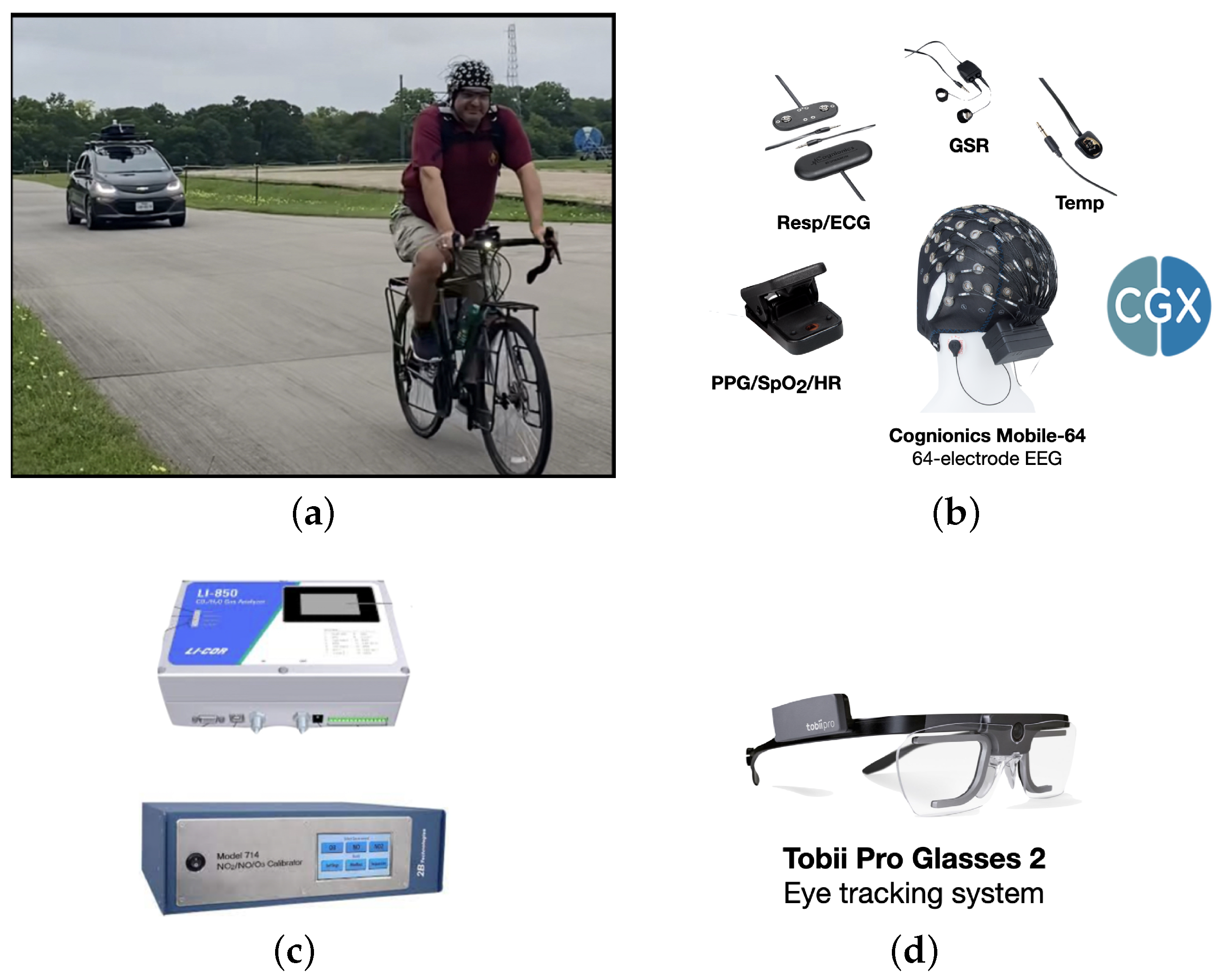
Figure 2.
(a and b) Location and track of bike ride where biometric variables and ambient concentration of , and NO were measured simultaneously. The arrow indicates the initial direction of the ride. The asterisk indicates the location where the data collection was started and ended.
Figure 2.
(a and b) Location and track of bike ride where biometric variables and ambient concentration of , and NO were measured simultaneously. The arrow indicates the initial direction of the ride. The asterisk indicates the location where the data collection was started and ended.
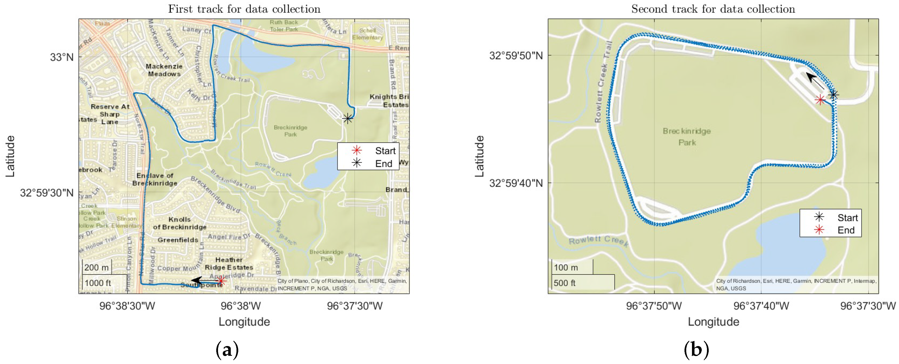
Figure 3.
A line graph of test RMSE in each of the 100 trial when physiological responses was first combined with PSD from ASA and then with PSD from WM to estimate inhaled concentration of: (a) , (b) and NO.
Figure 3.
A line graph of test RMSE in each of the 100 trial when physiological responses was first combined with PSD from ASA and then with PSD from WM to estimate inhaled concentration of: (a) , (b) and NO.
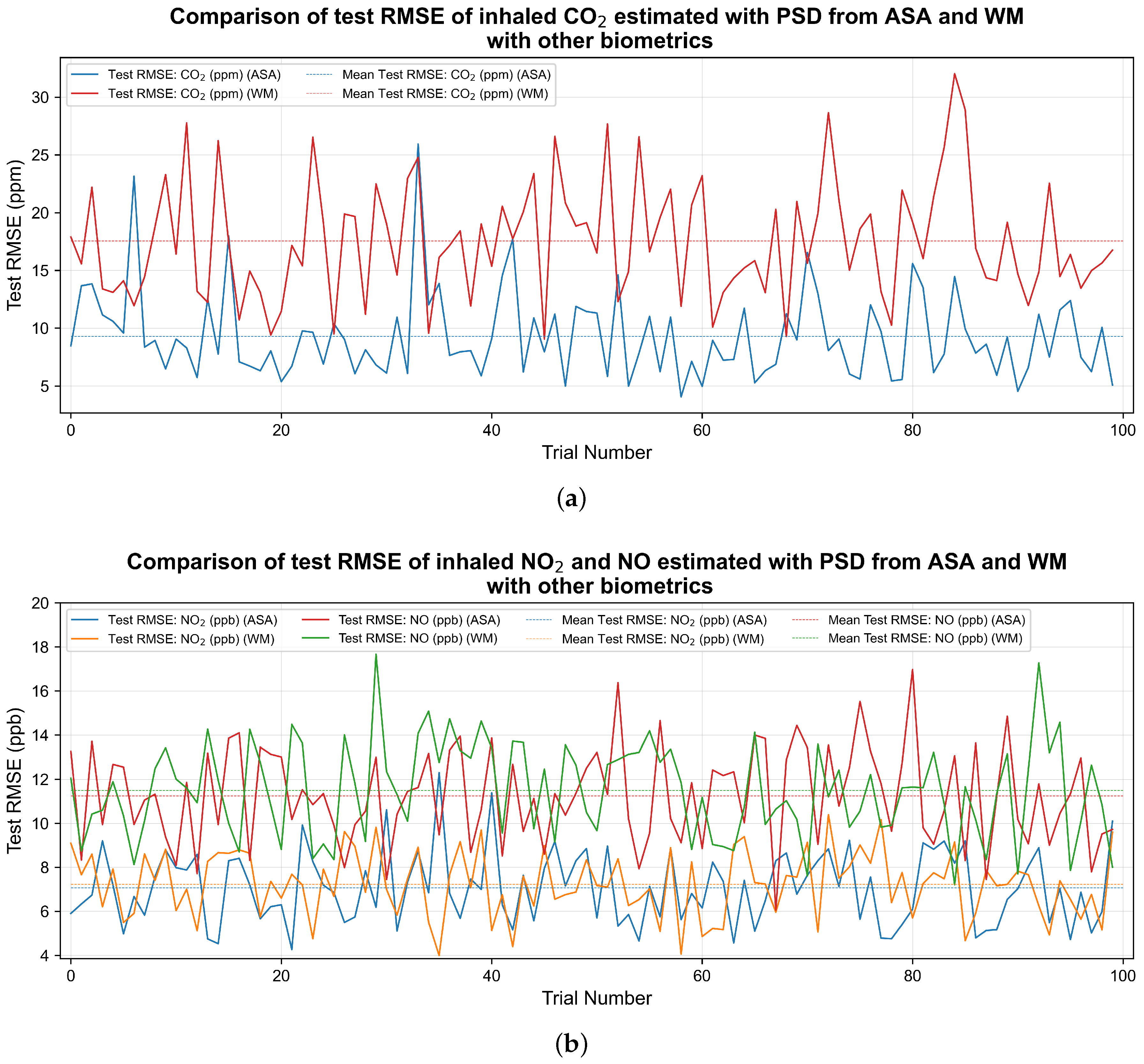
Figure 4.
A line graph of test of each of the 100 trial when physiological responses was first combined with PSD from ASA and then with PSD from WM for the case of: (a) and , (b) NO.
Figure 4.
A line graph of test of each of the 100 trial when physiological responses was first combined with PSD from ASA and then with PSD from WM for the case of: (a) and , (b) NO.
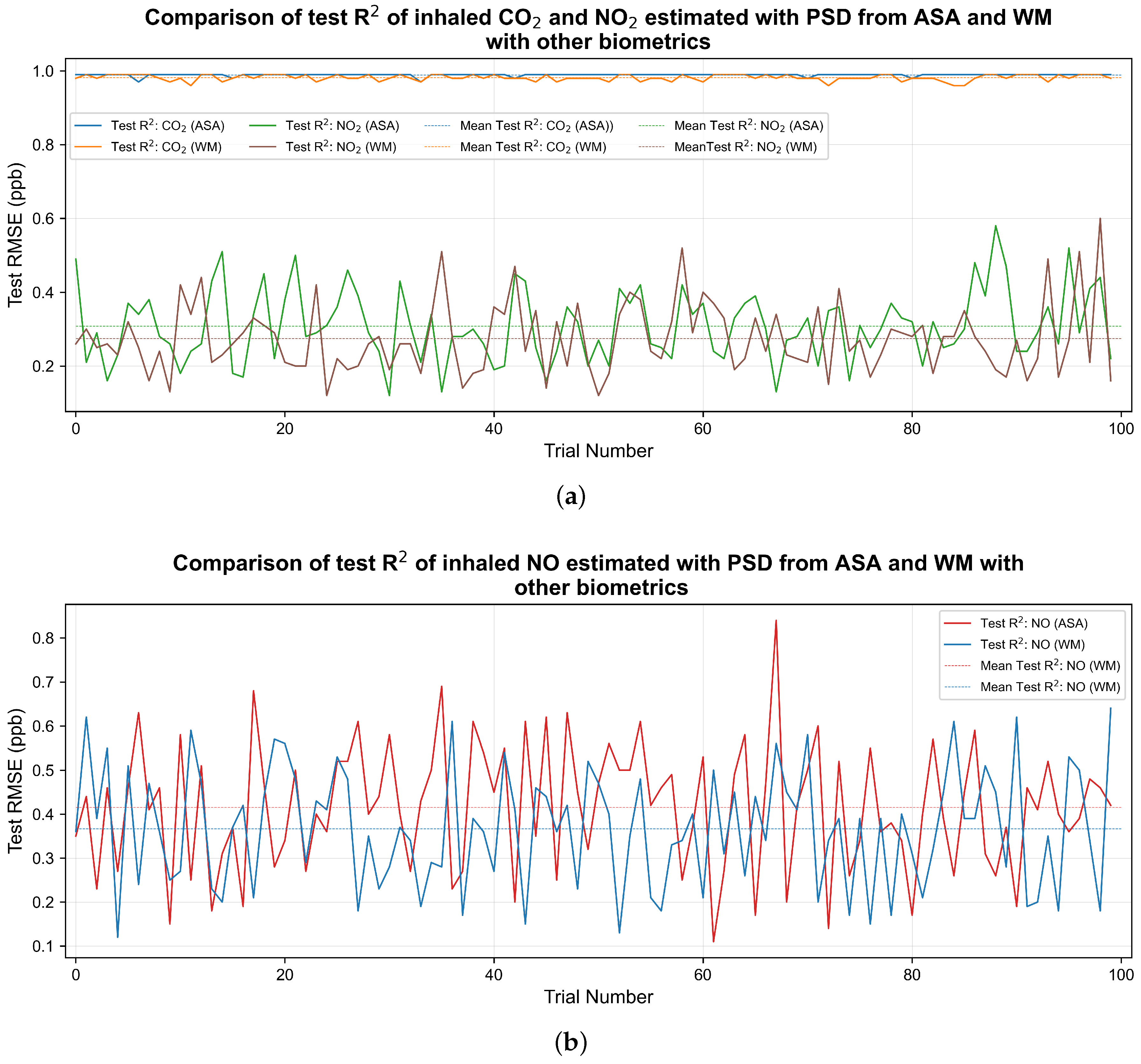
Figure 5.
An instance of scatter plot when physiological responses was combined with PSD from ASA for estimating inhaled concentration of (a) , (b) and (c) NO. An instance of scatter plot when physiological responses was combined with PSD from WM for estimating inhaled concentration of (a) , (b) and (c) NO. A perfect prediction is shown by the 1:1 line.
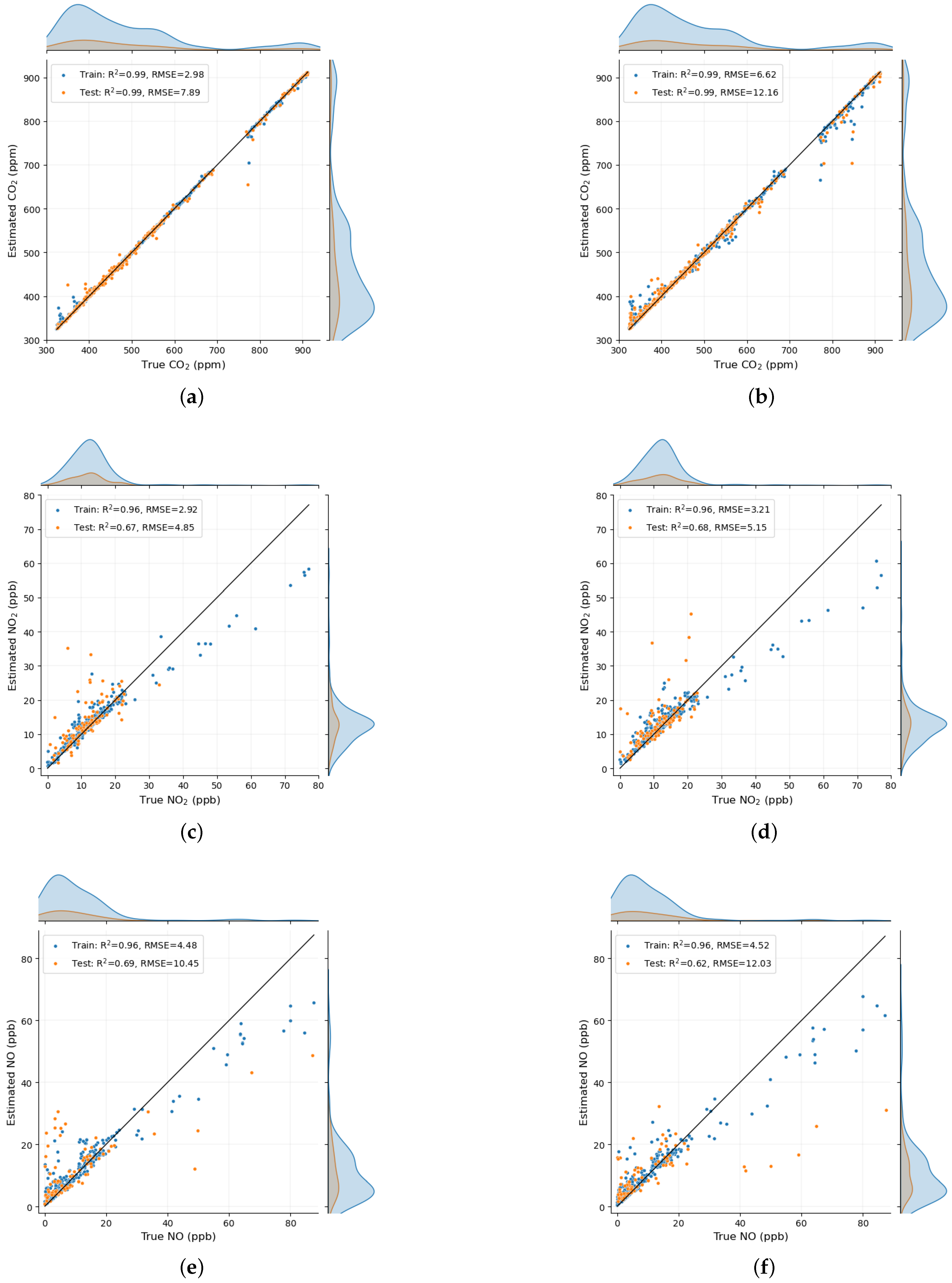
Figure 6.
An instance of Quantile-Quantile plot when physiological responses was combined with PSD from ASA for estimating inhaled concentration of (a) , (b) and (c) NO. An instance of Quantile-Quantile plot when physiological resoponses was combined with PSD from WM for estimating inhaled concentration of (a) , (b) and (c) NO. Two identical distribution will lie in the red 1:1 line.
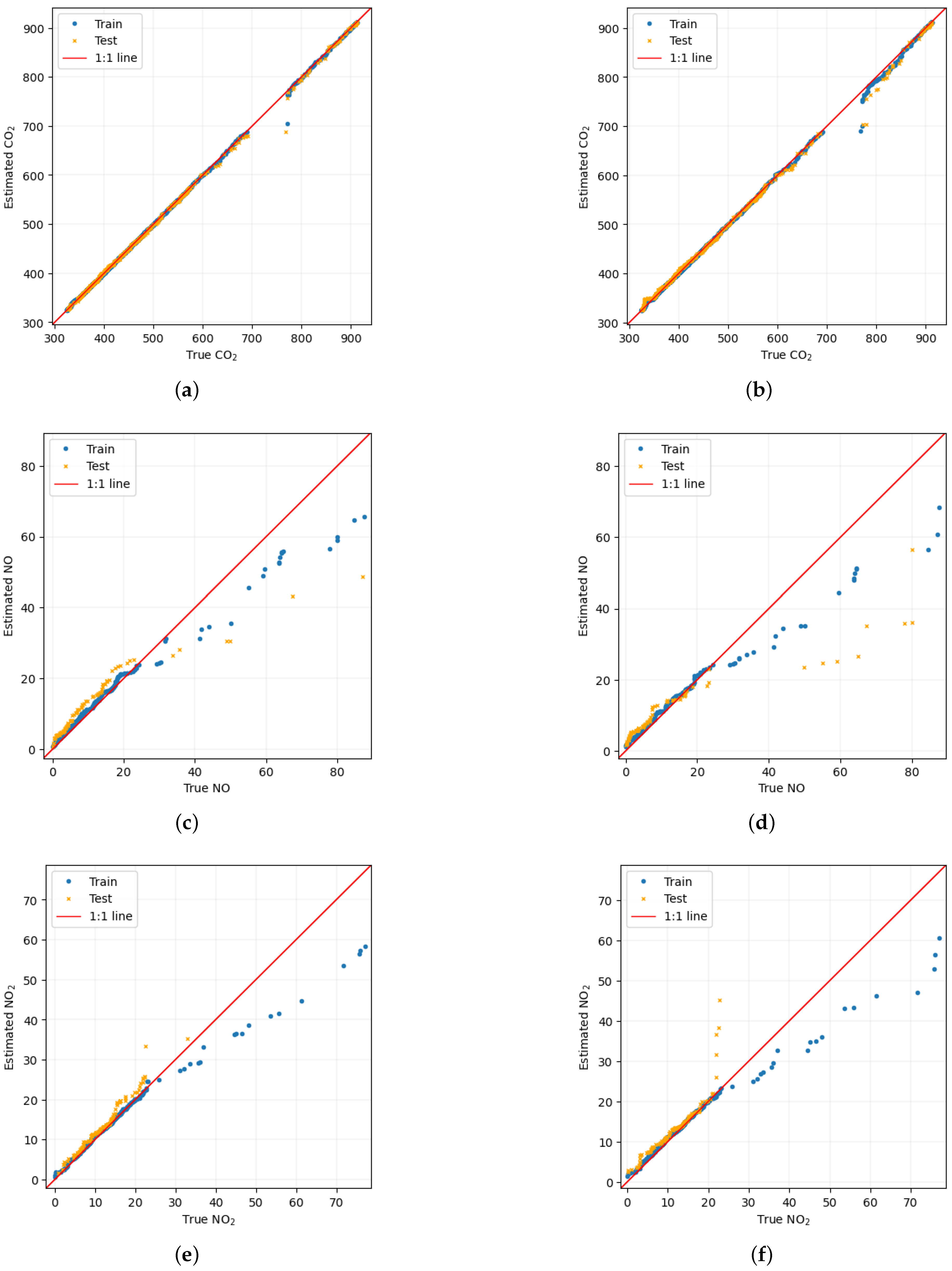
Figure 7.
Feature importance plot when physiological responses was combined with PSD from ASA for estimating inhaled concentration of (a) , (c) NO and (e) . Feature importance plot when physiological responses was combined with PSD from WM for estimating inhaled concentration of (b) , (d) NO and (f) .
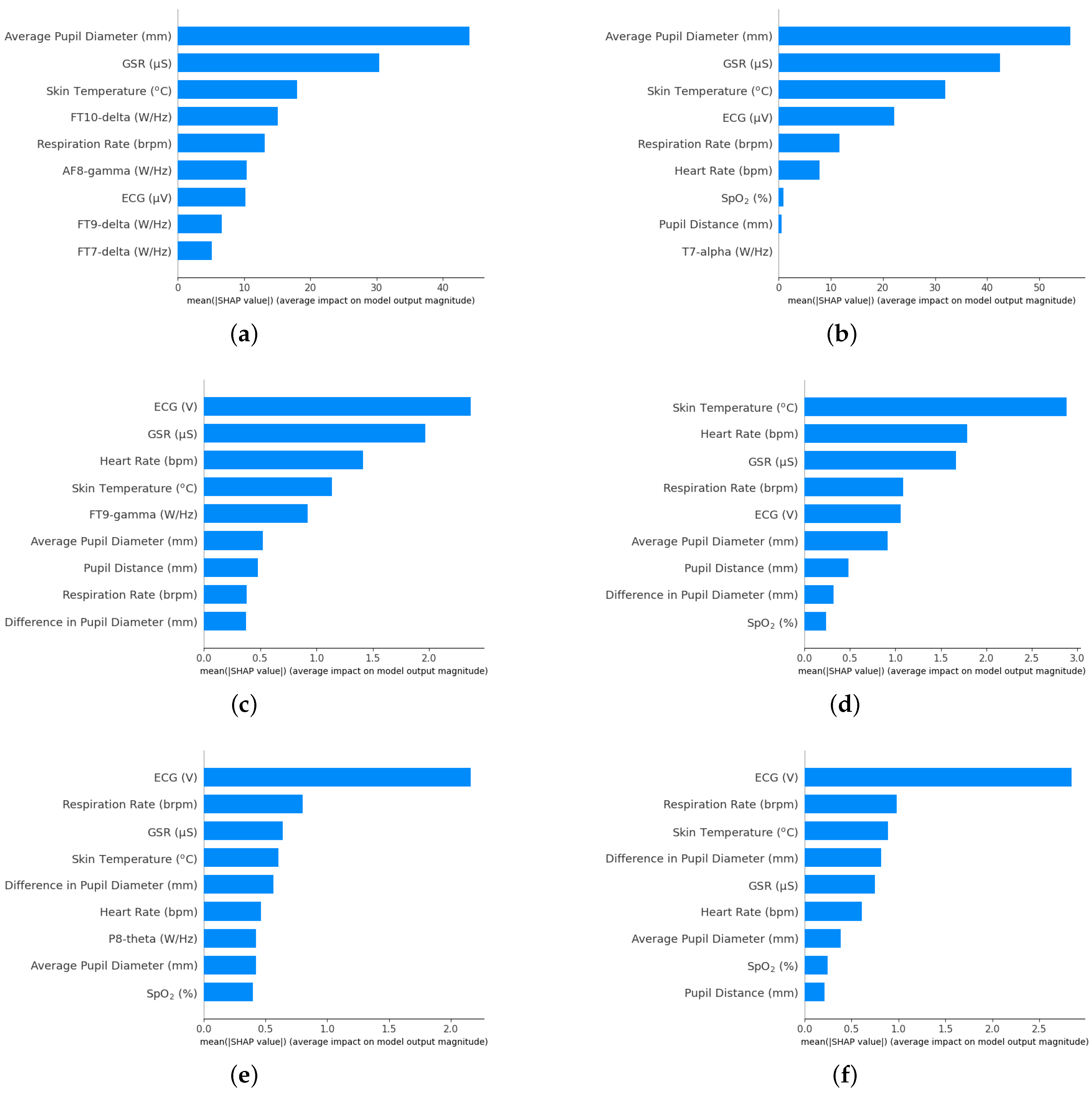
Table 1.
List of the biometric variables measured and corresponding units.
| Biometric Variable | Units |
|---|---|
| Electrical activities in brain using EEG | Volt (V) |
| Electrical activities in heart using ECG | Volt (V) |
| GSR | MicroSiemens (Siemens) |
| Percentage (%) | |
| Respiration rate | Breathing rate per minute (brpm) |
| Skin temperature | |
| Heart rate | Beats per minute (bpm) |
| Pupil diameter of each of the eyes | Millimeter (mm) |
| Distance between pupils | Millimeter (mm) |
Table 2.
Summary of data collection of , and NO.
| Pollutant | Total Number of Biometrics | Days of Data Collection | Number of Trials | Data Records in each Trial | Total Number of Data Records |
|---|---|---|---|---|---|
| 328 | 9 June, 10 June | 4 | 710, 696, 673, 238 | 2317 | |
| 328 | 26 May, 9 June, 10 June | 6 | 136, 23, 126, 120, 132, 45 | 582 | |
| NO | 328 | 26 May, 9 June, 10 June | 6 | 81, 15, 96, 88, 98, 32 | 410 |
Table 3.
Quantification of the estimation of pollutants in an independent test set using Random Forest with optimized hyperparameters after running the machine learning model 100 times.
Table 3.
Quantification of the estimation of pollutants in an independent test set using Random Forest with optimized hyperparameters after running the machine learning model 100 times.
| Pollutant | Average Test (PSD from WM) | Average Test (PSD from ASA) | Average Test RMSE (PSD from WM) | Average Test RMSE (PSD from ASA) |
|---|---|---|---|---|
| 0.98 | 0.98 | 17.55 ppm | 9.28 ppm | |
| NO | 0.36 | 0.41 | 11.50 ppb | 11.24 ppb |
| 0.27 | 0.30 | 7.23 ppb | 7.06 ppb |
Disclaimer/Publisher’s Note: The statements, opinions and data contained in all publications are solely those of the individual author(s) and contributor(s) and not of MDPI and/or the editor(s). MDPI and/or the editor(s) disclaim responsibility for any injury to people or property resulting from any ideas, methods, instructions or products referred to in the content. |
© 2024 by the authors. Licensee MDPI, Basel, Switzerland. This article is an open access article distributed under the terms and conditions of the Creative Commons Attribution (CC BY) license (http://creativecommons.org/licenses/by/4.0/).
Copyright: This open access article is published under a Creative Commons CC BY 4.0 license, which permit the free download, distribution, and reuse, provided that the author and preprint are cited in any reuse.


