
Submitted:
11 December 2024
Posted:
12 December 2024
You are already at the latest version
Abstract
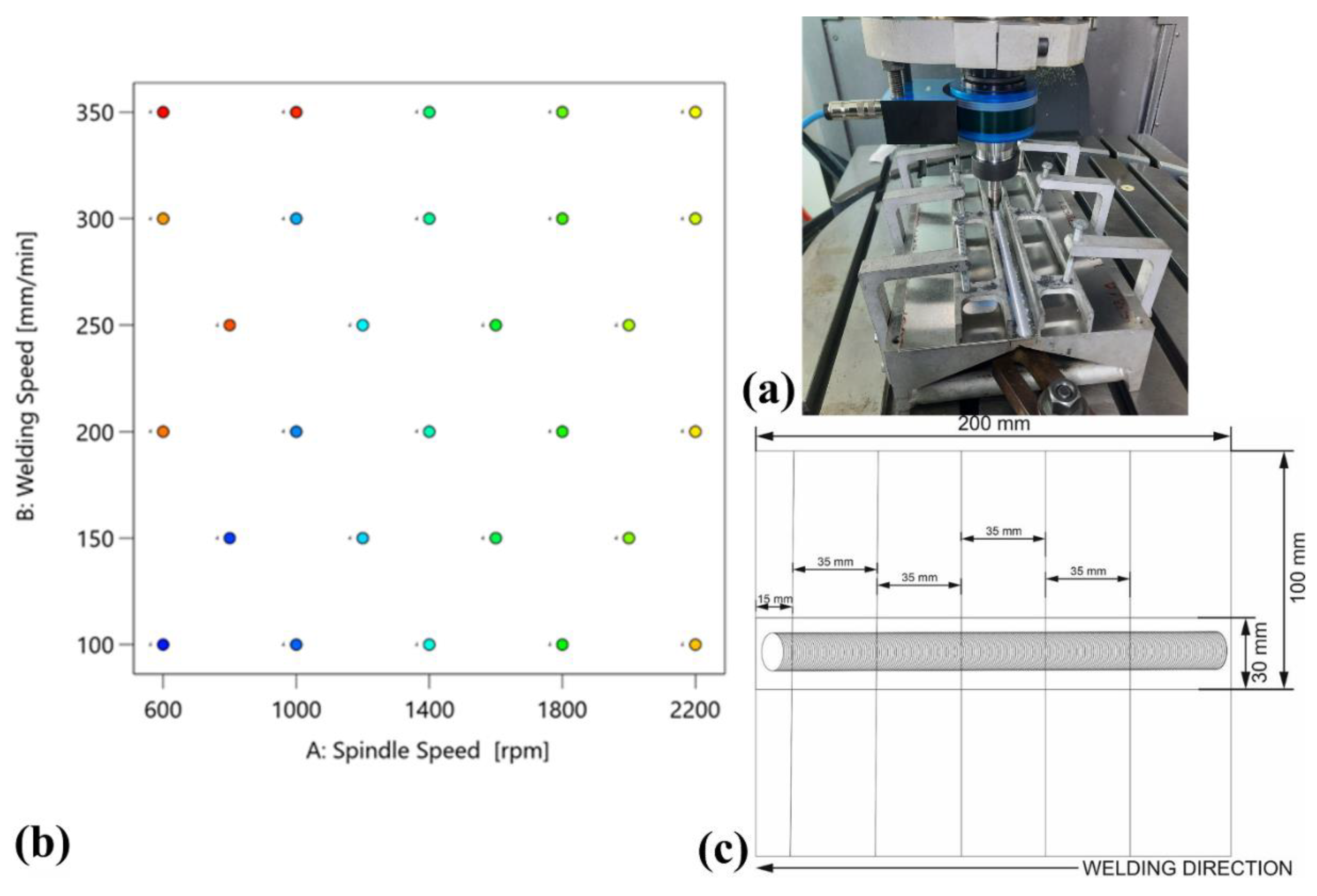
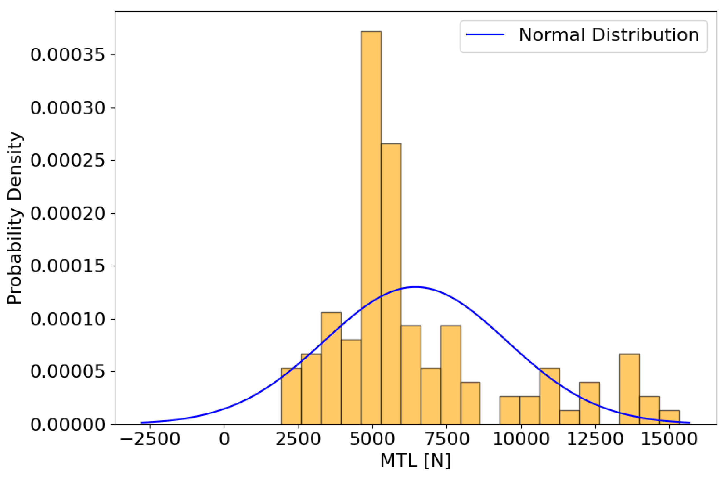
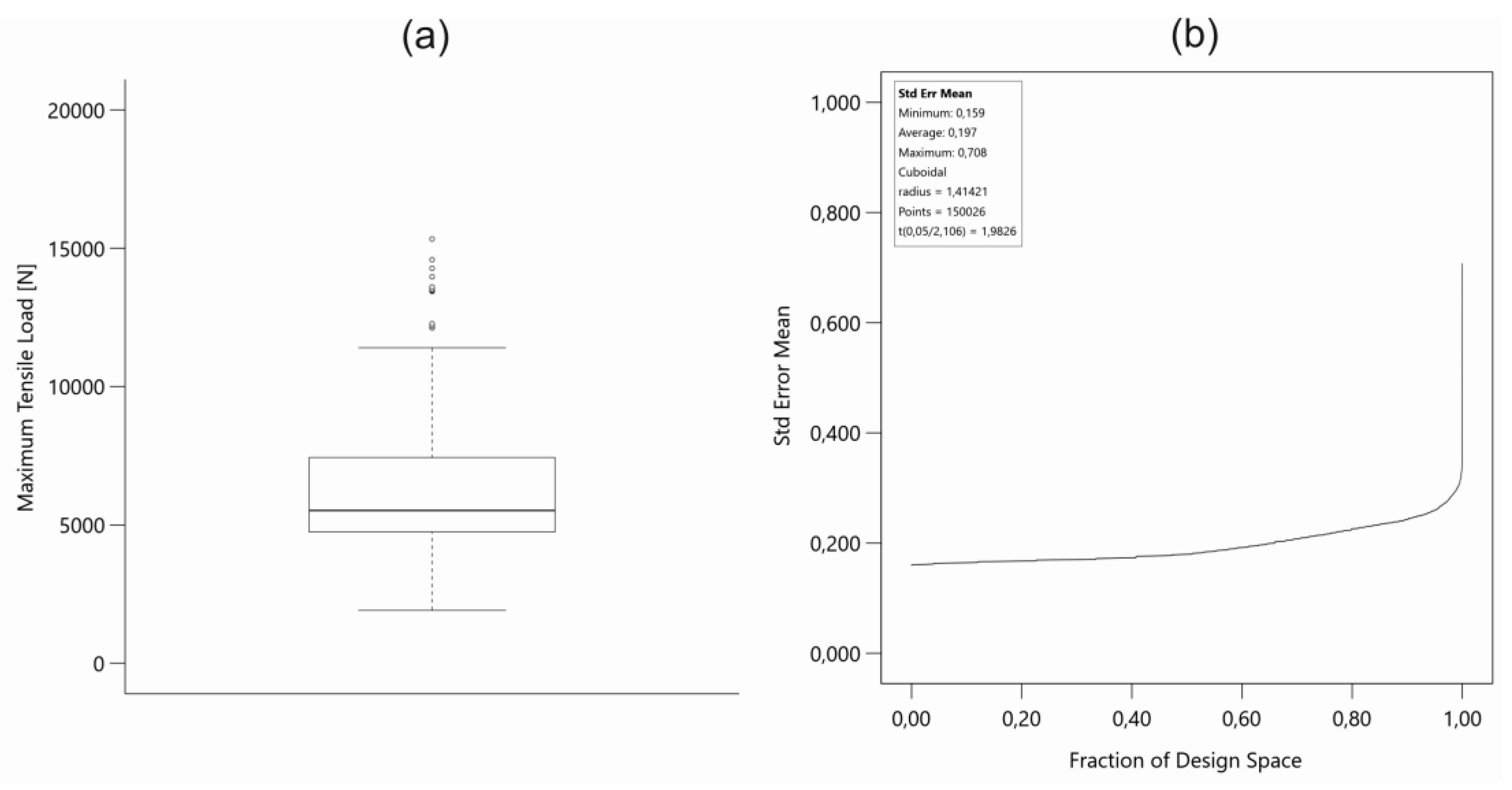
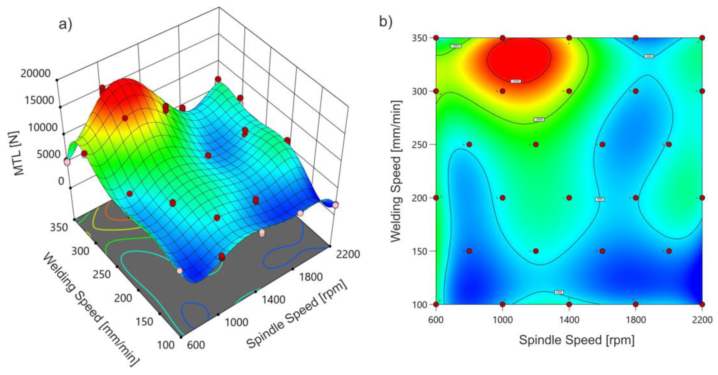
This study presents the optimization of the friction stir welding (FSW) process using polynomial regression to predict the maximum tensile load (MTL) of welded joints. The experimental design included varying spindle speeds from 600 to 2200 rpm and welding speeds from 100 to 350 mm/min over 28 experimental points. The resulting MTL values ranged from 1912 to 15336 N. A fifth degree polynomial regression model was developed to fit the experimental data. Diagnostic tests, including the Shapiro-Wilk test and kurtosis analysis, indicated a non-normal distribution of the MTL data. Model validation showed that fifth-degree polynomial regression provided a robust fit with high fitted and predicted R² values, indicating strong predictive power. Hill-climbing optimization was used to fine-tune the welding parameters, identifying an optimal spindle speed of 1100 rpm and a welding speed of 332 mm/min, which was predicted to achieve an MTL of 16852 N. Response surface analysis confirmed the effectiveness of the identified parameters and demonstrated their significant influence on the MTL. These results suggest that the applied polynomial regression model and optimization approach are effective tools for improving the performance and reliability of the FSW process.
Keywords:
1. Introduction
2. Materials and Methods
2.1. Evaluation of the Experimental Model
3. Creating a Polynomial Regression Model
3.1. Principles of Polynomial Regression
3.2. ANOVA for Fifth Model
4. Results
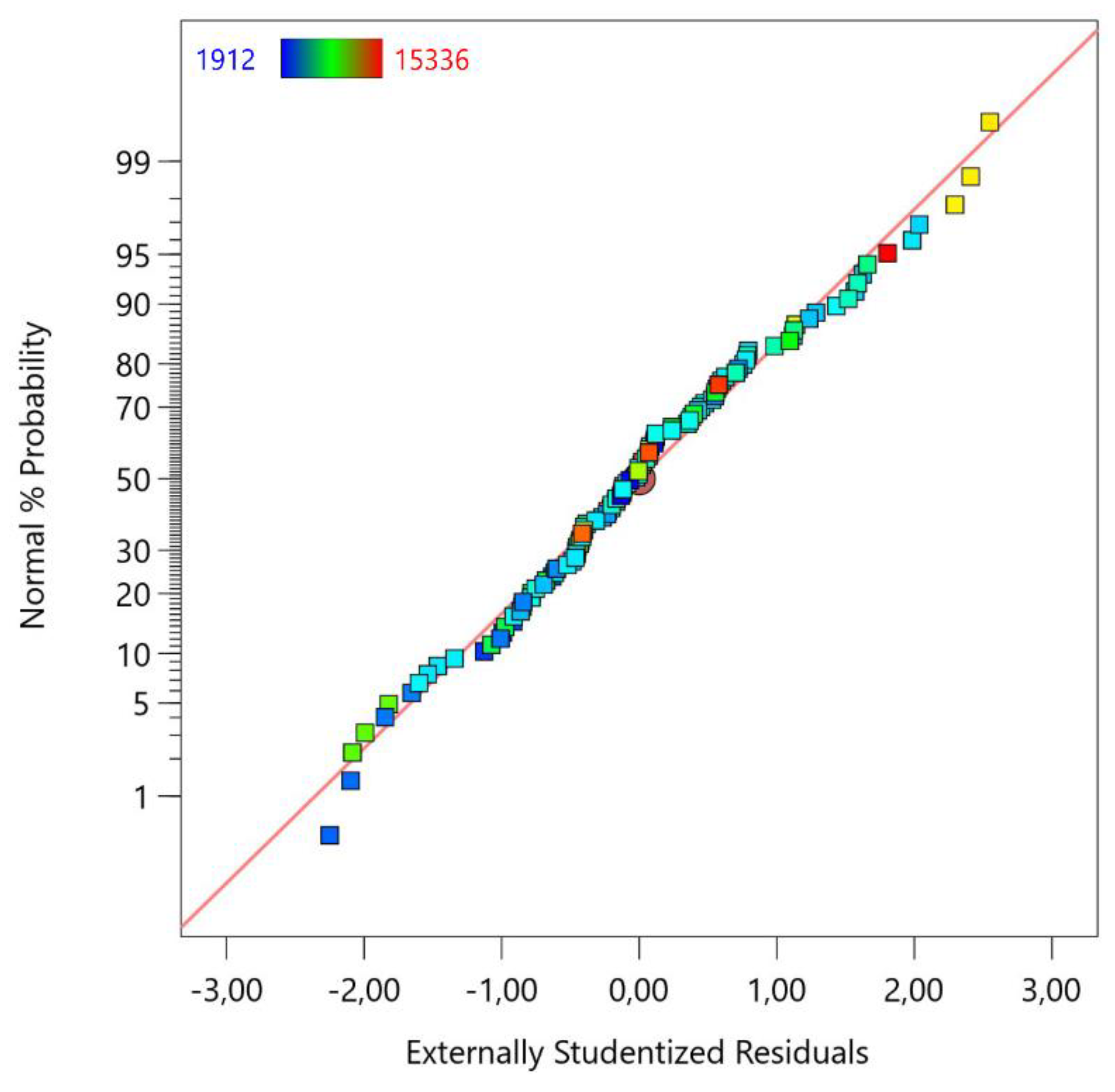
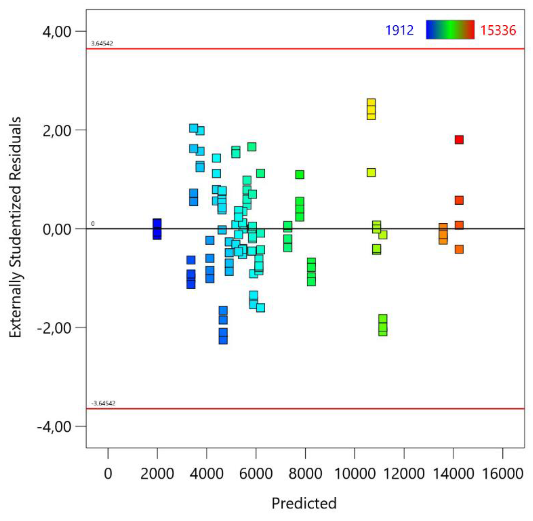
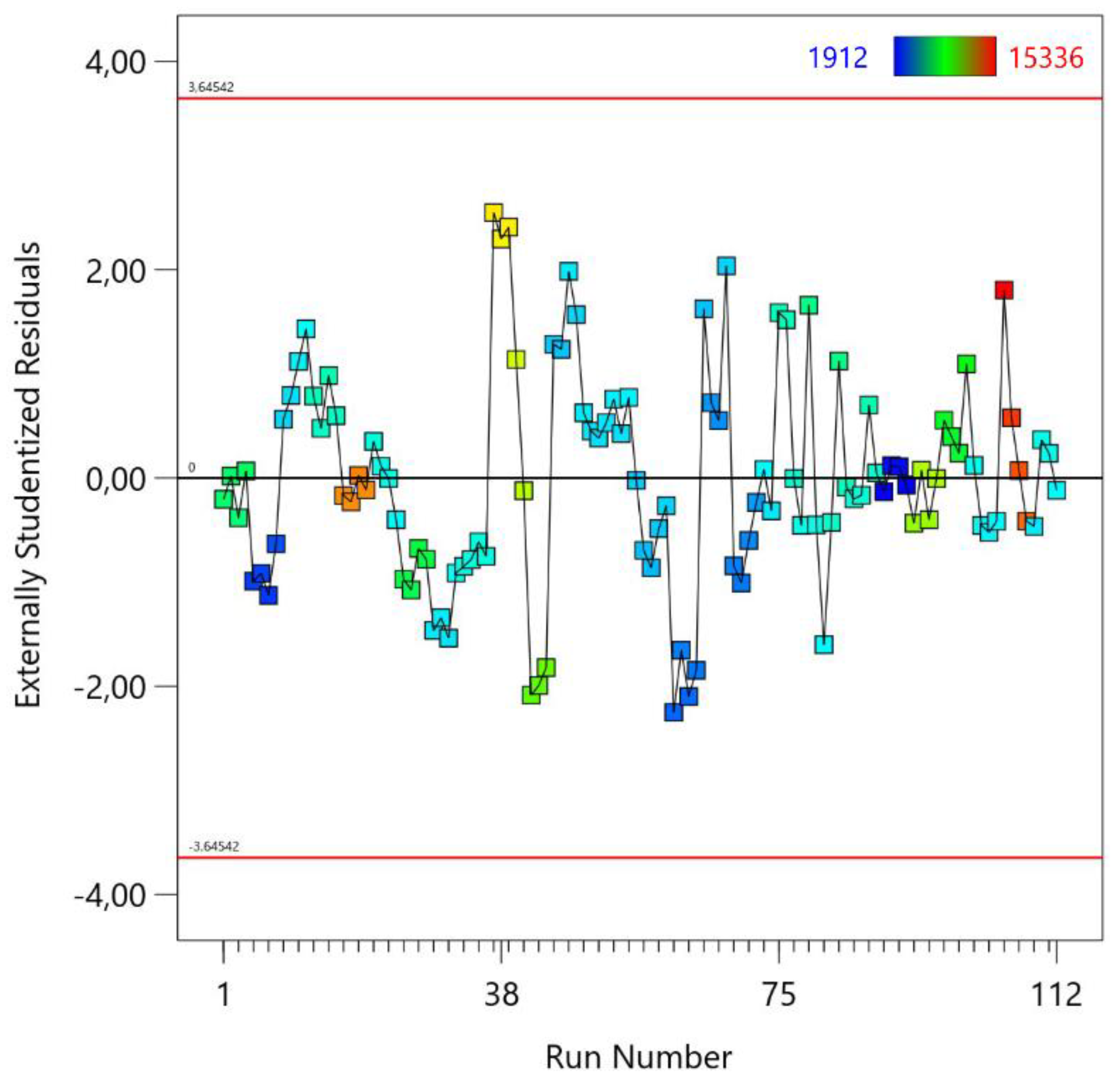
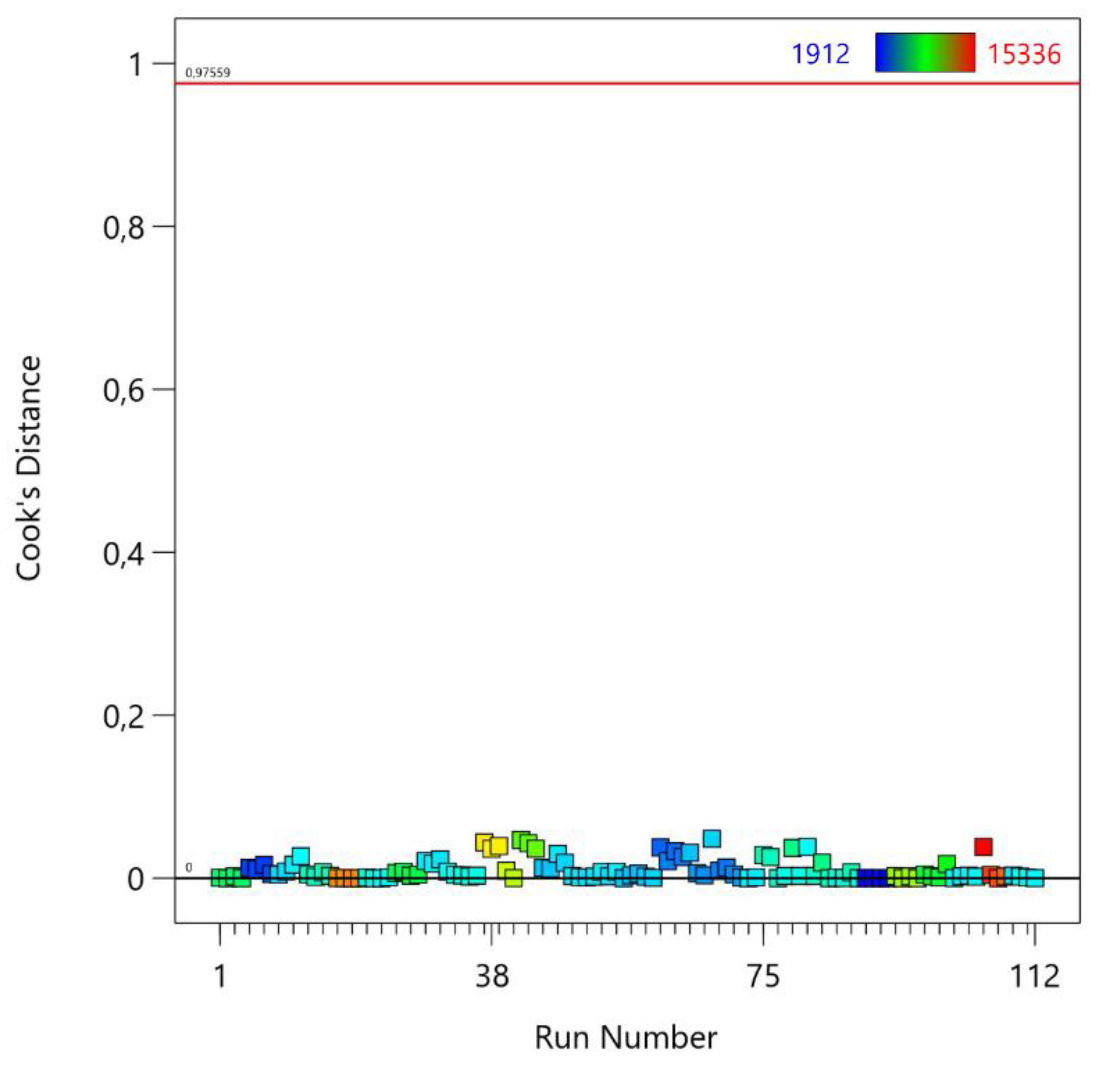
4.2. Model Diagnostics
4.2. Principles of Hill Climbing Algorithm
5. Optimization
6. Confirmation Test
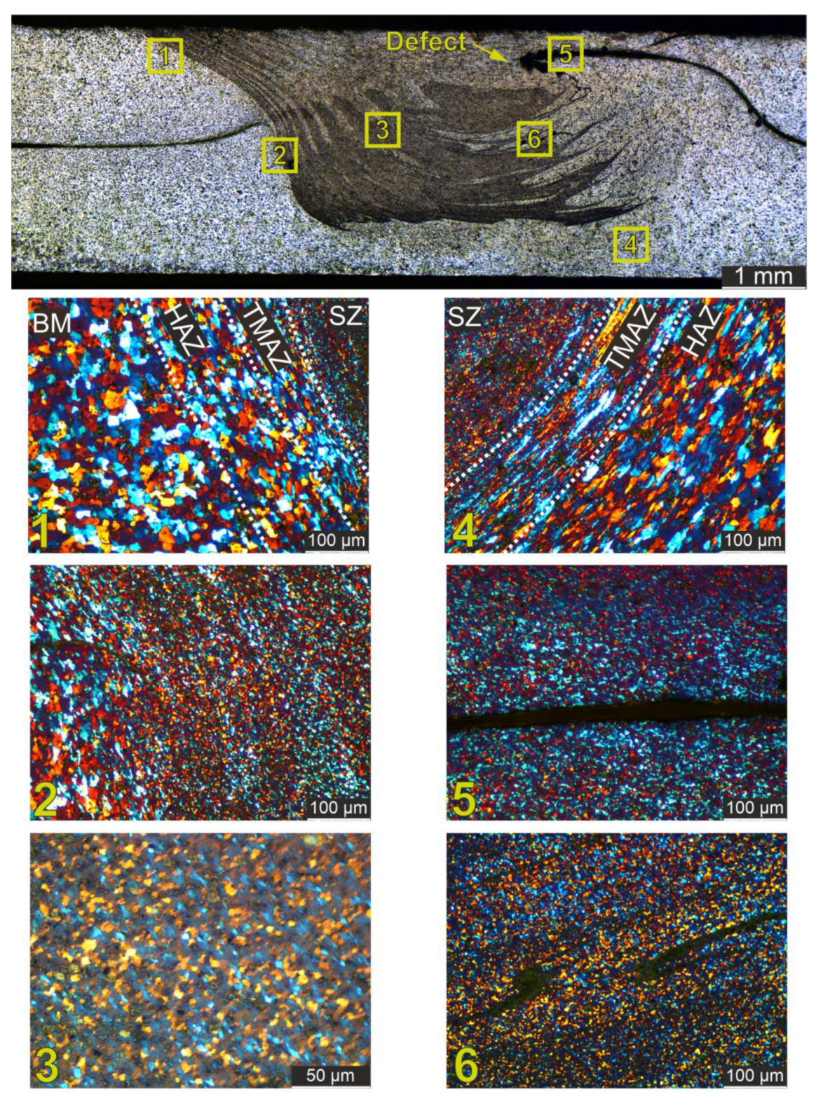
6.1. Macro and Microstructure Analysis
- Region 1 (Base Metal (BM), Heat Affected Zone (HAZ), Thermo-Mechanically Affected Zone (TMAZ), and Stir Zone (SZ)). This region shows the transition from the BM through the HAZ and the TMAZ into the SZ. The microstructure shows a gradual refinement of the grains from the BM to the SZ, indicating effective thermal and mechanical processing during FSW. The distinct zones highlight the gradient of thermal and mechanical effects on the material [21].
- Region 2 (TMAZ, HAZ): Similar to Region 1, this region provides a detailed view of the microstructural changes within the TMAZ and the HAZ. Grain refinement is evident as the material moves toward the stir zone, showing the progressive effect of the welding process on the material structure. The shape of the grains is a direct result of the compression process, which flattens them into small fractions and also causes further grain refinement. A similar evolution of the microstructure was shown in the work of Orlowska et al. [22].
- Region 3 (SZ): The stir zone exhibits a uniform and refined grain structure, indicating effective material mixing and recrystallization during the welding process. This region confirms the high quality of the stir zone, which is critical to the integrity and strength of the weld.
- Region 4 (SZ, TMAZ, HAZ): This region illustrates the microstructural characteristics at the interface between the stir zone (SZ), thermomechanically affected zone (TMAZ), and heat-affected zone (HAZ). The boundaries are well defined and demonstrate the effectiveness of the welding parameters in producing a strong joint with distinct zones that contribute to the overall mechanical properties of the weld.
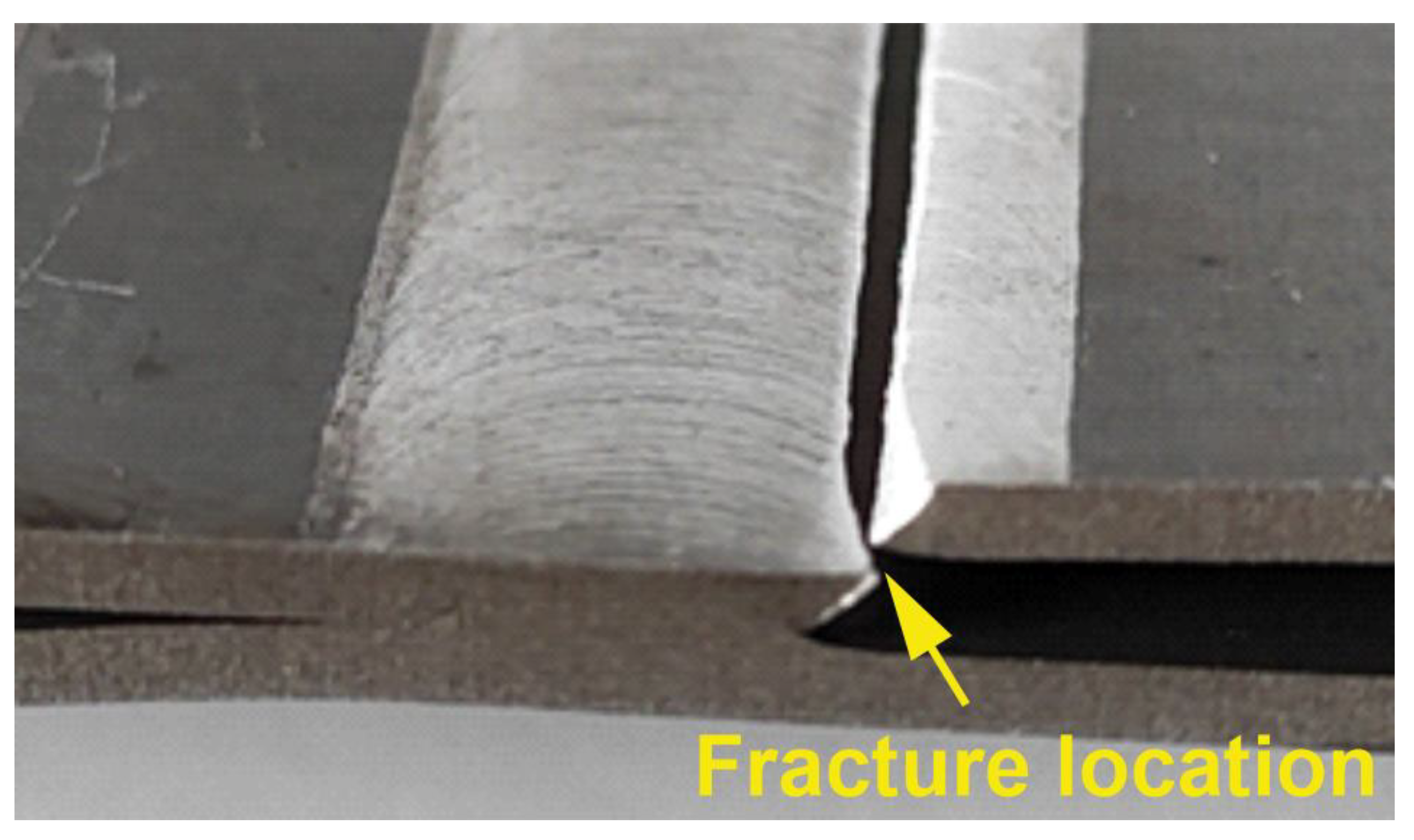
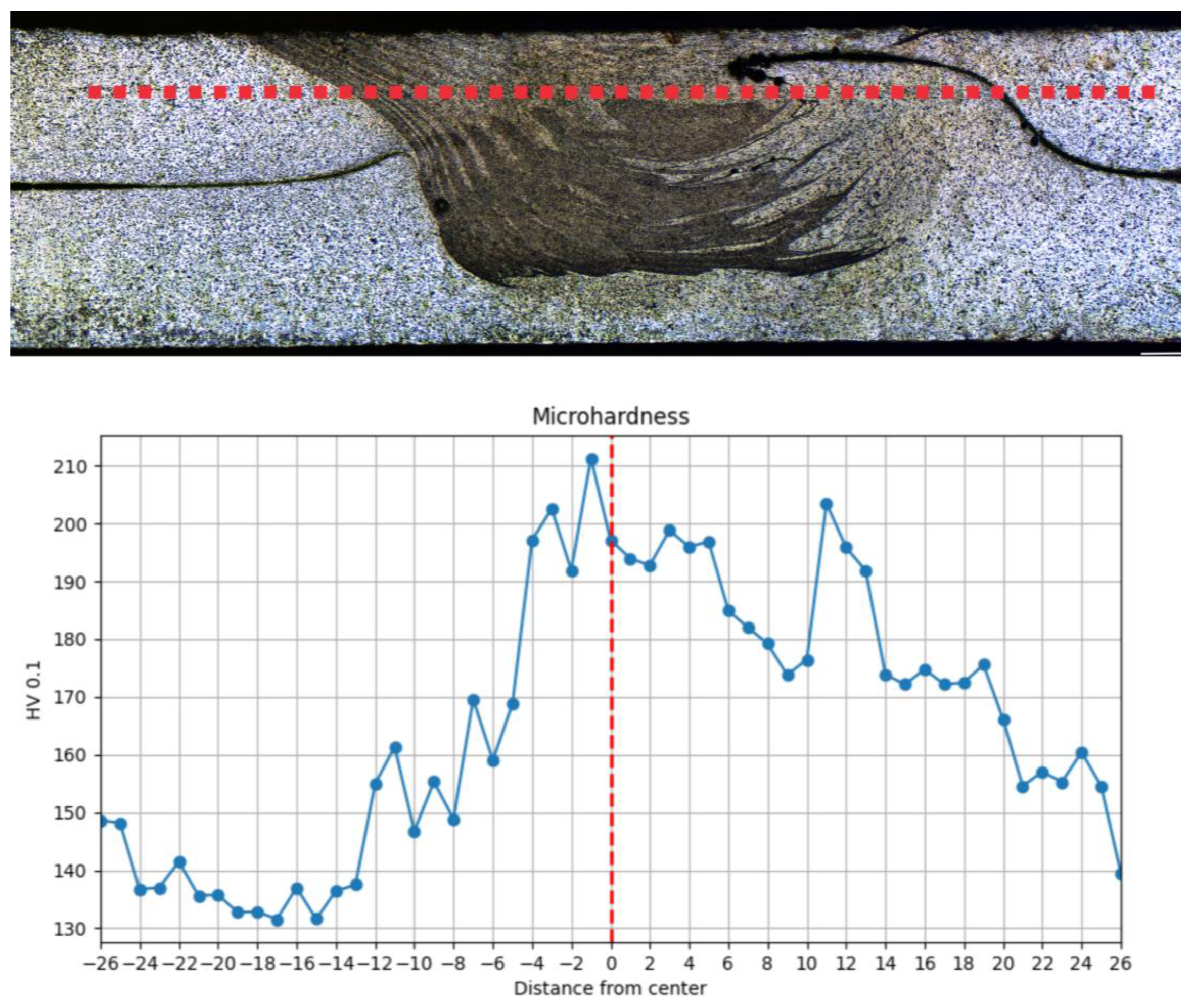
- Region 5 (SZ - Hooking): This section shows a hooking defect within the SZ. The hooking defect is characterized by a curved, hook-like shape at the interface between the joined materials. [23]. Despite the presence of this defect, the overall grain structure remains consistent with the expected characteristics of a properly welded stir zone. The hooking defect is identified during mechanical testing as a potential crack initiation site that can compromise the structural integrity of the weld.
- Region 6 (SZ - Material Flow Lines): The microstructure in this region shows material flow lines within the stir zone (SZ). The visible lines are likely flow lines of the material, with changes in shading possibly reflecting the presence of “onion rings” that are characteristic of FSW. These features indicate effective stirring and mixing of the material without the presence of cracks, confirming the overall quality of the weld in this region [24].
6.2. The Microhardness Analysis
7. Conclusions
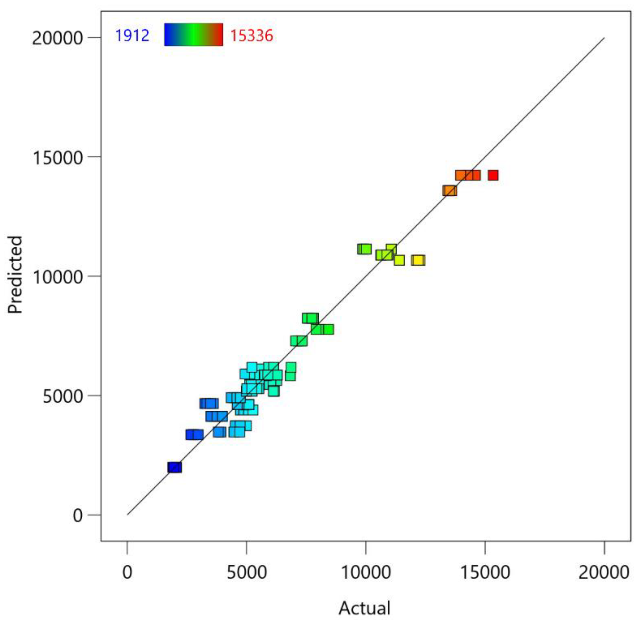
- A fifth-degree polynomial regression model was successfully developed to predict the maximum tensile load (MTL) of friction stir welded (FSW) joints, demonstrating high predictive accuracy with robust model performance and minimal overfitting.
- Experimental results showed MTL values ranging from 1912 to 15336 N over various spindle and welding speeds. Diagnostic tests indicated a non-normal distribution of MTL values, requiring robust model validation.
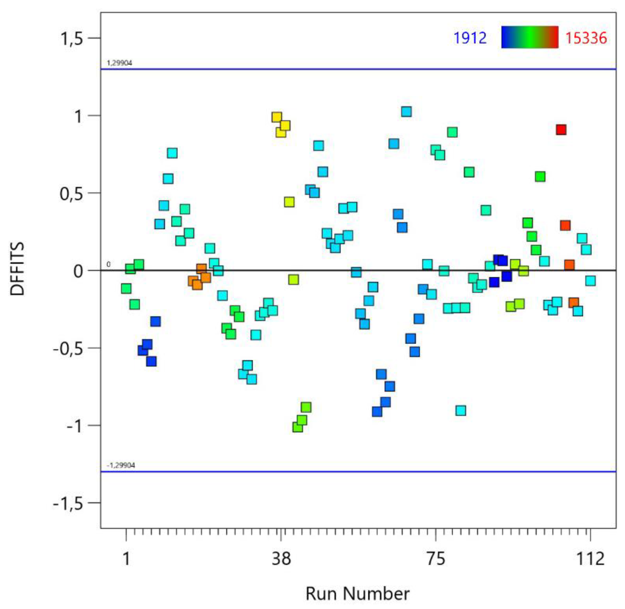
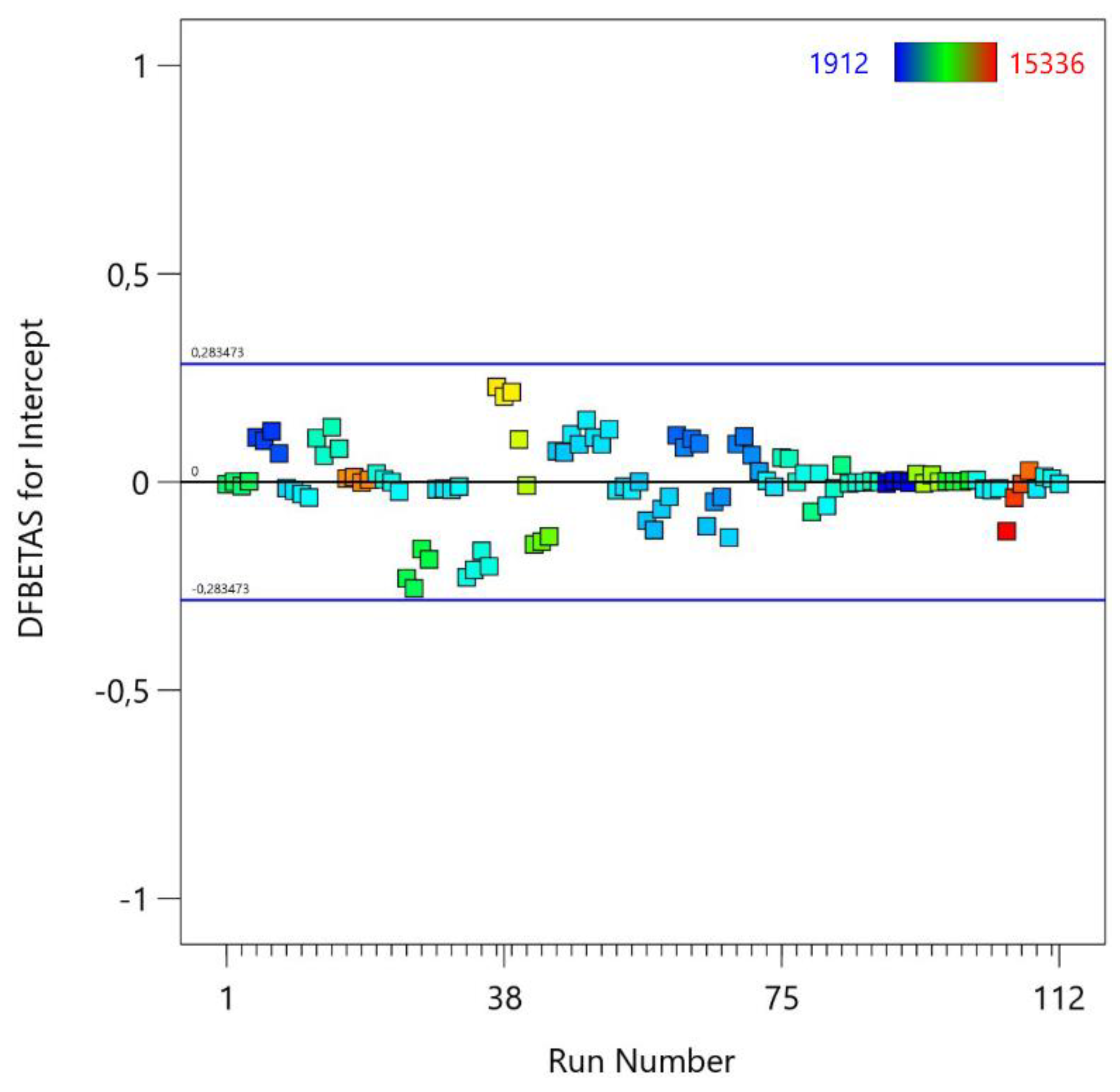
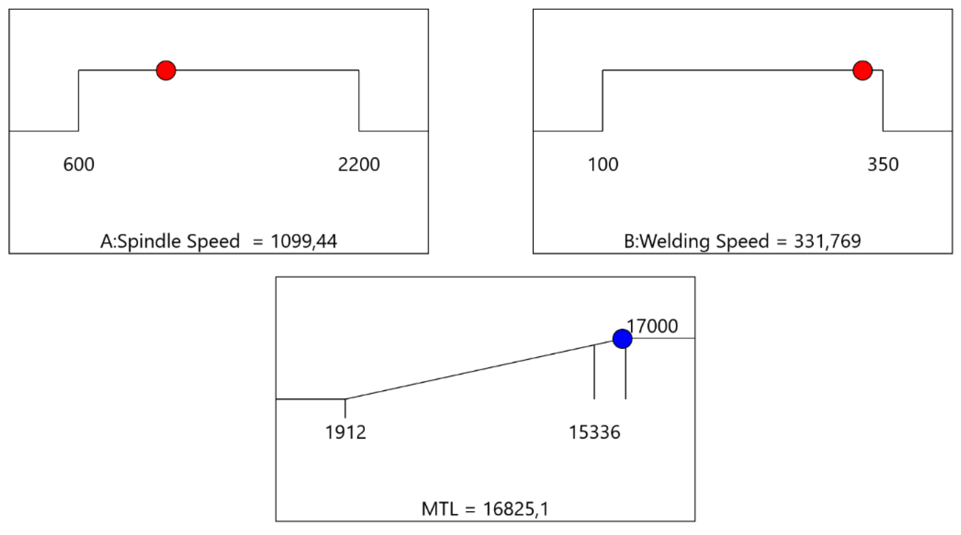
- Hill-climbing optimization effectively identified optimal welding parameters: a spindle speed of 1100 rpm and a welding speed of 332 mm/min, predicting an MTL of 16852 N. Diagnostic plots confirmed the model’s fit, ensuring reliable and robust predictions.
- The response surface plot validated the optimization results, highlighting regions of maximum MTL values corresponding to the identified optimal parameters. The interaction between spindle speed and welding speed was clearly demonstrated, showing their combined effect on MTL.
- The confirmation test validated the optimized parameters, achieving the predicted load capacities and demonstrating robust weld quality through detailed macro and microstructural examination.
- The microhardness profile of the FSW lap joint for AA2024-T3 alloy showed higher hardness in the weld nugget compared to the base material, with peak microhardness reaching approximately 210 HV in the weld center. This significant increase in microhardness is attributed to grain refinement and the absence of phase dissolution, indicating superior strength and hardness of the welded joint.
Author Contributions
Funding
Institutional Review Board Statement
Informed Consent Statement
Data Availability Statement
Conflicts of Interest
References
- Thomas, W.M.; Nicholas, E.D.; Needham, J.C.; Murch, M.G.; Temple-Smith, P.; Dawes, C.J. Friction Stir Welding. International Patent Application No. PCT/GB92/02203, 10 December 1991.
- Colligan, K.J. The Friction Stir Welding Process: An Overview. Friction Stir Welding; ; Elsevier: Amsterdam, The Netherlands, 2010; pp. 15–41. [CrossRef]
- Jamalian, H.M.; Tamjidi Eskandar, M.; Chamanara, A.; Karimzadeh, R.; Yousefian, R. An Artificial Neural Network Model for Multi-Pass Tool Pin Varying FSW of AA5086-H34 Plates Reinforced with Al2O3 Nanoparticles and Optimization for Tool Design Insight. CIRP J. Manuf. Sci. Technol. 2021, 35, 69–79. [CrossRef]
- Maleki, E. Artificial Neural Networks Application for Modeling of Friction Stir Welding Effects on Mechanical Properties of 7075-T6 Aluminum Alloy. IOP Conf. Ser. Mater. Sci. Eng. 2015, 103, 012034. [CrossRef]
- Myśliwiec, P.; Kubit, A.; Szawara, P. Optimization of 2024-T3 Aluminum Alloy Friction Stir Welding Using Random Forest, XGBoost, and MLP Machine Learning Techniques. Materials 2024, 17, 71452. [CrossRef]
- Vijayan, S.; Raju, R.; Subbaiah, K.; Sridhar, N.; Rao, S.R.K. Friction Stir Welding of Al-Mg Alloy Optimization of Process Parameters Using Taguchi Method. Exp. Tech. 2010, 34, 37–44. [CrossRef]
- Ravindrannair, P.; Equbal, A.; Equbal, Md.A.; Saxena, K.K.; Equbal, Md.I. Grey Based Taguchi Method for Multi-Response Optimization of FSW of Aluminium AA6061 Alloy. Int. J. Interact. Des. Manuf. IJIDeM 2024, 18, 1279–1290. [CrossRef]
- Karumuri, S.; Karri, K.; Abburu, R.; Kumar, A. Multi-Objective Optimization Using Taguchi Based Grey Relational Analysis in Friction Stir Welding for Dissimilar Aluminium Alloy. Int. J. Interact. Des. Manuf. IJIDeM 2024, 18, 1627–1644. [CrossRef]
- Silva, A.C.F.; Braga, D.F.O.; De Figueiredo, M.A.V.; Moreira, P.M.G.P. Ultimate Tensile Strength Optimization of Different FSW Aluminium Alloy Joints. Int. J. Adv. Manuf. Technol. 2015, 79, 805–814. [CrossRef]
- Verma, S.; Misra, J.P.; Gupta, M. Study of Temperature Distribution and Parametric Optimization During FSW of AA6082 Using Statistical Approaches. SAE Int. J. Mater. Manuf. 2019, 12, 73–82. [CrossRef]
- Zhang, F.; Li, L.; Han, Z.; Wang, X. Determination Method of Binary Fractions by the Integrated Spectrum. Mon. Not. R. Astron. Soc. 2024, 531, 3468–3478. [CrossRef]
- James, G.; Witten, D.; Hastie, T.; Tibshirani, R. An Introduction to Statistical Learning, 2nd ed.; Springer: New York, NY, USA, 2013. [CrossRef]
- Li, Y.; Li, M.; Zhang, L. Evolutionary Polynomial Regression Improved by Regularization Methods. PLoS ONE 2023, 18, e0282029. [CrossRef]
- Marasco, S.; Marano, G.C.; Cimellaro, G.P. Evolutionary Polynomial Regression Algorithm Combined with Robust Bayesian Regression. Adv. Eng. Softw. 2022, 167, 103101. [CrossRef]
- Cheng, C.-L.; Tsai, J.-R.; Schneeweiss, H. Polynomial Regression with Heteroscedastic Measurement Errors in Both Axes: Estimation and Hypothesis Testing. Stat. Methods Med. Res. 2019, 28, 2681–2696. [CrossRef]
- Sulthan, A.; Jayakumar, G.S.D.S. Exact Distribution of Cook’s Distance and Identification of Influential Observations. Hacet. J. Math. Stat. 2014, 44, 1–1. [CrossRef]
- Li, J.; Valliant, R. Linear Regression Influence Diagnostics for Unclustered Survey Data. J. Off. Stat. 2011, 27, 99–119.
- Bahadir, B.; İnci, H.; Karadavut, U. Determination of Outlier in Live-Weight Performance Data of Japanese Quails (Coturnix Coturnix Japonica) by DFBETA and DFBETAS Techniques. Ital. J. Anim. Sci. 2014, 13, 3113. [CrossRef]
- Kuznetsov, A.; Abusukhon, A.; Andreev, K.; Sidorov, I.; Pavlova, V. Optimizing Hill Climbing Algorithm for S-Boxes Generation. Electronics 2023, 12, 2338. [CrossRef]
- Peker, F.; Altun, M. A Fast Hill Climbing Algorithm for Defect and Variation Tolerant Logic Mapping of Nano-Crossbar Arrays. IEEE Trans. Multi-Scale Comput. Syst. 2018, 4, 522–532. [CrossRef]
- Qiao, J.; Shi, Q.; Chen, S.; Yang, C.; Han, Y.; Chen, G. Visualization of Vertical Transfer of Material Through High-Velocity Rotating Flow Zone During Friction Stir Welding. Mater. Lett. 2024, 367, 136599. [CrossRef]
- Orłowska, M.; Mrozek, K.; Kaczmarek, L.; Sidor, J.; Staniek, A. Local Changes in the Microstructure, Mechanical and Electrochemical Properties of Friction Stir Welded Joints from Aluminium of Varying Grain Size. J. Mater. Res. Technol. 2021, 15, 5968–5987. [CrossRef]
- Ji, S.; Li, Z. Reducing the Hook Defect of Friction Stir Lap Welded Ti-6Al-4V Alloy by Slightly Penetrating into the Lower Sheet. J. Mater. Eng. Perform. 2017, 26, 921–930. [CrossRef]
- Yang, C.; Li, Y.; Zhang, J.; Gao, Z.; Wu, X. Material Flow During Dissimilar Friction Stir Welding of Al/Mg Alloys. Int. J. Mech. Sci. 2024, 272, 109173. [CrossRef]
- Myśliwiec, P.; Śliwa, R.E.; Ostrowski, R. Friction Stir Welding of Ultrathin AA2024-T3 Aluminum Sheets Using Ceramic Tool. Arch. Met. Mater. 2019, 64, 1385–1394.
- Myśliwiec, P.; Śliwa, R.E. Friction Stir Welding of Thin Sheets of the AA2024-T3 Alloy with a Ceramic Tool: RSM and ANOVA Study. Key Eng. Mater. 2022, 926, 1756–1761. [CrossRef]
- Salih, O.S.; Neate, N.; Ou, H.; Sun, W. Influence of Process Parameters on the Microstructural Evolution and Mechanical Characterisations of Friction Stir Welded Al-Mg-Si Alloy. J. Mater. Process. Technol. 2020, 275, 116366. [CrossRef]
- Laska, A.; Szkodo, M.; Cavaliere, P.; Moszczyńska, D.; Mizera, J. Analysis of Residual Stresses and Dislocation Density of AA6082 Butt Welds Produced by Friction Stir Welding. Metall. Mater. Trans. A 2023, 54, 211–225. [CrossRef]
- Sato, Y.S.; Urata, M.; Kokawa, H.; Ikeda, K. Hall–Petch Relationship in Friction Stir Welds of Equal Channel Angular-Pressed Aluminium Alloys. Mater. Sci. Eng. A 2003, 354, 298–305. [CrossRef]
- Kosturek, R.; Śnieżek, L.; Torzewski, J.; Wachowski, M. Research on the Friction Stir Welding of Sc-Modified AA2519 Extrusion. Metals 2019, 9, 1024. [CrossRef]
- Staron, P.; Kocak, M.; Williams, S. Residual Stresses in Friction Stir Welded Al Sheets. Appl. Phys. Mater. Sci. Process. 2002, 74, s1161–s1162. [CrossRef]

| Tool Parameters | Value | Tool View |
|---|---|---|
| Shoulder diameter D [mm] | 12 | 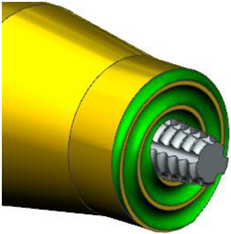 |
| Pin diameter d [mm] | 4.5 | |
| Pin height [mm] | 2.55 | |
| Tool offset [mm] | 0.05 | |
| Dwell time [s] | 10 | |
| Tool tilt angle | 0° | |
| Tool plunge speed [mm/min] | 2 | |
| Shoulder profile | Flat with spiral groove | |
| Pin profile | Conical threaded | |
| D/d ratio of the tool | 2.7 | |
| Tool material | H13 Steel |
| Factor | Name | Units | Type | Min. | Max. | Coded Low | Coded High | Mean | Std. Dev. |
|---|---|---|---|---|---|---|---|---|---|
| A | Spindle Speed | rpm | Numeric | 600 | 2200 | -1 ↔ 600 | +1 ↔ 2200 | 1400 | 536.92 |
| B | Welding Speed | N | Numeric | 100 | 350 | -1 ↔ 100 | +1 ↔ 350 | 226.79 | 87.49 |
| Response | Name | Units | Observations | Min. | Max. | Mean | Std. Dev. | Ratio |
|---|---|---|---|---|---|---|---|---|
| R1 | MTL | N | 112 | 1912 | 15336 | 6451.97 | 3071.58 | 8.02 |
| Term | Standard Error* | VIF | Rᵢ² | Power |
|---|---|---|---|---|
| A | 0.1416 | 1.00309 | 0.0031 | 99.9 % |
| B | 0.1357 | 1.00182 | 0.0018 | 99.9 % |
| AB | 0.1964 | 1.00309 | 0.0031 | 99.9 % |
| A² | 0.2453 | 1.01148 | 0.0114 | 99.9 % |
| B² | 0.2349 | 1.00965 | 0.0096 | 99.9 % |
| Source | Sequential p-Value |
Lack of Fit p-Value |
Adjusted R² | Predicted R² | |
|---|---|---|---|---|---|
| Linear | < 0.0001 | < 0.0001 | 0.3877 | 0.3629 | |
| 2FI | 0.1962 | < 0.0001 | 0.3916 | 0.3541 | |
| Quadratic | 0.1153 | < 0.0001 | 0.4049 | 0.3573 | |
| Cubic | < 0.0001 | < 0.0001 | 0.5213 | 0.4544 | |
| Quartic | < 0.0001 | < 0.0001 | 0.8435 | 0.8234 | |
| Fifth | < 0.0001 | < 0.0001 | 0.9489 | 0.9390 | Suggested |
| Sixth | < 0.0001 | < 0.0001 | 0.9752 | 0.9683 | Aliased |
| Source | Sum of Squares | df | Mean Square | F-Value | p-Value | |
|---|---|---|---|---|---|---|
| Model | 1.003E+09 | 20 | 5.017E+07 | 104.12 | < 0.0001 | significant |
| A-Spindle Speed | 3.854E+07 | 1 | 3.854E+07 | 79.99 | < 0.0001 | |
| B-Welding Speed | 7.292E+05 | 1 | 7.292E+05 | 1.51 | 0.2218 | |
| AB | 1.535E+08 | 1 | 1.535E+08 | 318.49 | < 0.0001 | |
| A² | 1.946E+07 | 1 | 1.946E+07 | 40.40 | < 0.0001 | |
| B² | 2.012E+07 | 1 | 2.012E+07 | 41.77 | < 0.0001 | |
| A²B | 1.090E+06 | 1 | 1.090E+06 | 2.26 | 0.1360 | |
| AB² | 4.119E+07 | 1 | 4.119E+07 | 85.49 | < 0.0001 | |
| A³ | 4.509E+07 | 1 | 4.509E+07 | 93.59 | < 0.0001 | |
| B³ | 1.284E+07 | 1 | 1.284E+07 | 26.65 | < 0.0001 | |
| A²B² | 3.609E+07 | 1 | 3.609E+07 | 74.91 | < 0.0001 | |
| A³B | 1.930E+08 | 1 | 1.930E+08 | 400.65 | < 0.0001 | |
| AB³ | 5.528E+06 | 1 | 5.528E+06 | 11.47 | 0.0010 | |
| A⁴ | 2.486E+07 | 1 | 2.486E+07 | 51.60 | < 0.0001 | |
| B⁴ | 8.687E+06 | 1 | 8.687E+06 | 18.03 | < 0.0001 | |
| A³B² | 1.317E+07 | 1 | 1.317E+07 | 27.33 | < 0.0001 | |
| A²B³ | 51117.18 | 1 | 51117.18 | 0.1061 | 0.7454 | |
| A⁴B | 50177.92 | 1 | 50177.92 | 0.1041 | 0.7477 | |
| AB⁴ | 2.440E+07 | 1 | 2.440E+07 | 50.64 | < 0.0001 | |
| A⁵ | 4.439E+07 | 1 | 4.439E+07 | 92.12 | < 0.0001 | |
| B⁵ | 1.765E+07 | 1 | 1.765E+07 | 36.62 | < 0.0001 | |
| Residual | 4.385E+07 | 91 | 4.818E+05 | |||
| Lack of Fit | 3.533E+07 | 7 | 5.048E+06 | 49.80 | < 0.0001 | significant |
| Pure Error | 8.514E+06 | 84 | 1.014E+05 | |||
| Cor Total | 1.047E+09 | 111 |
| Std. Dev. | 694.15 | R² | 0.9581 |
| Mean | 6451.97 | Adjusted R² | 0.9489 |
| C.V. % | 10.76 | Predicted R² | 0.9390 |
| Adeq Precision | 40.7155 |
| MTL | = |
|---|---|
| +2.65761E+05 | |
| -816.24439 | Spindle Speed |
| -1633.38459 | Welding Speed |
| -2.37849 | Spindle Speed * Welding Speed |
| +1.42349 | Spindle Speed ² |
| +24.68195 | Welding Speed² |
| +0.000460 | Spindle Speed ² * Welding Speed |
| +0.016034 | Spindle Speed * Welding Speed² |
| -0.001068 | Spindle Speed ³ |
| -0.158386 | Welding Speed³ |
| -2.71047E-06 | Spindle Speed ² * Welding Speed² |
| -4.74309E-08 | Spindle Speed ³ * Welding Speed |
| -0.000039 | Spindle Speed * Welding Speed³ |
| +3.80250E-07 | Spindle Speed ⁴ |
| +0.000442 | Welding Speed⁴ |
| +5.20073E-10 | Spindle Speed ³ * Welding Speed² |
| +2.29939E-10 | Spindle Speed ² * Welding Speed³ |
| -7.12925E-12 | Spindle Speed ⁴ * Welding Speed |
| +4.38557E-08 | Spindle Speed * Welding Speed⁴ |
| -5.22195E-11 | Spindle Speed ⁵ |
| -4.58801E-07 | Welding Speed⁵ |
| Run Order |
Rotational Speed [rpm] | Welding Speed [mm/min] | Actual Value of MTL [N] | Predicted Value of MTL [N] | Residual | Leverage | Internally Studentized Residuals | Externally Studentized Residuals | Cook’s Distance | Influence on Fitted Value DFFITS |
|---|---|---|---|---|---|---|---|---|---|---|
| 1 | 600 | 100 | 7165.00 | 7288.17 | -123.17 | 0.248 | -0.205 | -0.204 | 0.001 | -0.117 |
| 2 | 7299.00 | 7288.17 | 10.83 | 0.248 | 0.018 | 0.018 | 0.000 | 0.010 | ||
| 3 | 7057.00 | 7288.17 | -231.17 | 0.248 | -0.384 | -0.382 | 0.002 | -0.219 | ||
| 4 | 7329.00 | 7288.17 | 40.83 | 0.248 | 0.068 | 0.067 | 0.000 | 0.039 | ||
| 5 | 800 | 150 | 2754.00 | 3364.21 | -610.21 | 0.213 | -0.991 | -0.991 | 0.013 | -0.516 |
| 6 | 2800.00 | 3364.21 | -564.21 | 0.213 | -0.916 | -0.916 | 0.011 | -0.477 | ||
| 7 | 2671.00 | 3364.21 | -693.21 | 0.213 | -1.126 | -1.128 | 0.016 | -0.588 | ||
| 8 | 2974.00 | 3364.21 | -390.21 | 0.213 | -0.634 | -0.632 | 0.005 | -0.329 | ||
| 9 | 1000 | 100 | 4746.00 | 4397.76 | 348.24 | 0.218 | 0.567 | 0.565 | 0.004 | 0.299 |
| 10 | 4885.00 | 4397.76 | 487.24 | 0.218 | 0.794 | 0.792 | 0.008 | 0.419 | ||
| 11 | 5084.00 | 4397.76 | 686.24 | 0.218 | 1.118 | 1.120 | 0.017 | 0.592 | ||
| 12 | 5272.00 | 4397.76 | 874.24 | 0.218 | 1.425 | 1.433 | 0.027 | 0.757 | ||
| 13 | 1000 | 200 | 6138.00 | 5629.89 | 508.11 | 0.139 | 0.789 | 0.787 | 0.005 | 0.316 |
| 14 | 5938.00 | 5629.89 | 308.11 | 0.139 | 0.478 | 0.476 | 0.002 | 0.191 | ||
| 15 | 6264.00 | 5629.89 | 634.11 | 0.139 | 0.984 | 0.984 | 0.007 | 0.395 | ||
| 16 | 6017.00 | 5629.89 | 387.11 | 0.139 | 0.601 | 0.599 | 0.003 | 0.241 | ||
| 17 | 1000 | 300 | 13477.00 | 13585.93 | -108.93 | 0.141 | -0.169 | -0.168 | 0.000 | -0.068 |
| 18 | 13438.00 | 13585.93 | -147.93 | 0.141 | -0.230 | -0.229 | 0.000 | -0.093 | ||
| 19 | 13602.00 | 13585.93 | 16.07 | 0.141 | 0.025 | 0.025 | 0.000 | 0.010 | ||
| 20 | 13511.00 | 13585.93 | -74.93 | 0.141 | -0.116 | -0.116 | 0.000 | -0.047 | ||
| 21 | 1200 | 150 | 5692.00 | 5464.73 | 227.27 | 0.141 | 0.353 | 0.352 | 0.001 | 0.143 |
| 22 | 5538.00 | 5464.73 | 73.27 | 0.141 | 0.114 | 0.113 | 0.000 | 0.046 | ||
| 23 | 5462.00 | 5464.73 | -2.73 | 0.141 | -0.004 | -0.004 | 0.000 | -0.002 | ||
| 24 | 5206.00 | 5464.73 | -258.73 | 0.141 | -0.402 | -0.400 | 0.001 | -0.162 | ||
| 25 | 1200 | 250 | 7612.00 | 8243.00 | -631.00 | 0.128 | -0.973 | -0.973 | 0.007 | -0.373 |
| 26 | 7547.00 | 8243.00 | -696.00 | 0.128 | -1.074 | -1.075 | 0.008 | -0.411 | ||
| 27 | 7803.00 | 8243.00 | -440.00 | 0.128 | -0.679 | -0.677 | 0.003 | -0.259 | ||
| 28 | 7735.00 | 8243.00 | -508.00 | 0.128 | -0.784 | -0.782 | 0.004 | -0.299 | ||
| 29 | 1400 | 100 | 4984.00 | 5902.63 | -918.63 | 0.173 | -1.455 | -1.464 | 0.021 | -0.669 |
| 30 | 5059.00 | 5902.63 | -843.63 | 0.173 | -1.336 | -1.342 | 0.018 | -0.613 | ||
| 31 | 4939.00 | 5902.63 | -963.63 | 0.173 | -1.526 | -1.538 | 0.023 | -0.702 | ||
| 32 | 5326.00 | 5902.63 | -576.63 | 0.173 | -0.913 | -0.912 | 0.008 | -0.417 | ||
| 33 | 1400 | 200 | 5560.00 | 6117.56 | -557.56 | 0.106 | -0.850 | -0.848 | 0.004 | -0.292 |
| 34 | 5602.00 | 6117.56 | -515.56 | 0.106 | -0.786 | -0.784 | 0.003 | -0.270 | ||
| 35 | 5714.00 | 6117.56 | -403.56 | 0.106 | -0.615 | -0.613 | 0.002 | -0.211 | ||
| 36 | 5623.00 | 6117.56 | -494.56 | 0.106 | -0.754 | -0.752 | 0.003 | -0.259 | ||
| 37 | 1400 | 300 | 12271.00 | 10669.27 | 1601.73 | 0.131 | 2.475 | 2.549 | 0.044 | 0.989 |
| 38 | 12121.00 | 10669.27 | 1451.73 | 0.131 | 2.243 | 2.295 | 0.036 | 0.891 | ||
| 39 | 12189.00 | 10669.27 | 1519.73 | 0.131 | 2.348 | 2.410 | 0.040 | 0.935 | ||
| 40 | 11405.00 | 10669.27 | 735.73 | 0.131 | 1.137 | 1.139 | 0.009 | 0.442 | ||
| 41 | 1400 | 350 | 11064.00 | 11140.53 | -76.53 | 0.191 | -0.123 | -0.122 | 0.000 | -0.059 |
| 42 | 9862.00 | 11140.53 | -1278.53 | 0.191 | -2.047 | -2.084 | 0.047 | -1.011 | ||
| 43 | 9916.00 | 11140.53 | -1224.53 | 0.191 | -1.961 | -1.992 | 0.043 | -0.967 | ||
| 44 | 10018.00 | 11140.53 | -1122.53 | 0.191 | -1.797 | -1.820 | 0.036 | -0.883 | ||
| 45 | 1600 | 150 | 4556.00 | 3732.42 | 823.58 | 0.141 | 1.280 | 1.285 | 0.013 | 0.521 |
| 46 | 4525.00 | 3732.42 | 792.58 | 0.141 | 1.232 | 1.236 | 0.012 | 0.501 | ||
| 47 | 4989.00 | 3732.42 | 1256.58 | 0.141 | 1.953 | 1.985 | 0.030 | 0.805 | ||
| 48 | 4734.00 | 3732.42 | 1001.58 | 0.141 | 1.557 | 1.569 | 0.019 | 0.636 | ||
| 49 | 1600 | 250 | 5028.00 | 4620.71 | 407.29 | 0.128 | 0.628 | 0.626 | 0.003 | 0.240 |
| 50 | 4914.00 | 4620.71 | 293.29 | 0.128 | 0.452 | 0.450 | 0.001 | 0.172 | ||
| 51 | 4870.00 | 4620.71 | 249.29 | 0.128 | 0.385 | 0.383 | 0.001 | 0.147 | ||
| 52 | 4966.00 | 4620.71 | 345.29 | 0.128 | 0.533 | 0.531 | 0.002 | 0.203 | ||
| 53 | 1800 | 100 | 5092.00 | 4625.74 | 466.26 | 0.218 | 0.760 | 0.758 | 0.008 | 0.401 |
| 54 | 4889.00 | 4625.74 | 263.26 | 0.218 | 0.429 | 0.427 | 0.002 | 0.226 | ||
| 55 | 5102.00 | 4625.74 | 476.26 | 0.218 | 0.776 | 0.774 | 0.008 | 0.409 | ||
| 56 | 4612.00 | 4625.74 | -13.74 | 0.218 | -0.022 | -0.022 | 0.000 | -0.012 | ||
| 57 | 1800 | 200 | 4465.00 | 4913.36 | -448.36 | 0.139 | -0.696 | -0.694 | 0.004 | -0.279 |
| 58 | 4357.00 | 4913.36 | -556.36 | 0.139 | -0.864 | -0.863 | 0.006 | -0.347 | ||
| 59 | 4599.00 | 4913.36 | -314.36 | 0.139 | -0.488 | -0.486 | 0.002 | -0.195 | ||
| 60 | 4741.00 | 4913.36 | -172.36 | 0.139 | -0.268 | -0.266 | 0.001 | -0.107 | ||
| 61 | 1800 | 300 | 3250.00 | 4666.11 | -1416.11 | 0.141 | -2.201 | -2.250 | 0.038 | -0.912 |
| 62 | 3612.00 | 4666.11 | -1054.11 | 0.141 | -1.638 | -1.654 | 0.021 | -0.670 | ||
| 63 | 3341.00 | 4666.11 | -1325.11 | 0.141 | -2.060 | -2.098 | 0.033 | -0.850 | ||
| 64 | 3493.00 | 4666.11 | -1173.11 | 0.141 | -1.823 | -1.847 | 0.026 | -0.749 | ||
| 65 | 1800 | 350 | 4472.00 | 3473.27 | 998.73 | 0.202 | 1.611 | 1.625 | 0.031 | 0.818 |
| 66 | 3922.00 | 3473.27 | 448.73 | 0.202 | 0.724 | 0.722 | 0.006 | 0.363 | ||
| 67 | 3816.00 | 3473.27 | 342.73 | 0.202 | 0.553 | 0.551 | 0.004 | 0.277 | ||
| 68 | 4715.00 | 3473.27 | 1241.73 | 0.202 | 2.003 | 2.037 | 0.048 | 1.025 | ||
| 69 | 2000 | 150 | 3611.00 | 4131.38 | -520.38 | 0.213 | -0.845 | -0.844 | 0.009 | -0.440 |
| 70 | 3511.00 | 4131.38 | -620.38 | 0.213 | -1.008 | -1.008 | 0.013 | -0.525 | ||
| 71 | 3761.00 | 4131.38 | -370.38 | 0.213 | -0.602 | -0.600 | 0.005 | -0.312 | ||
| 72 | 3987.00 | 4131.38 | -144.38 | 0.213 | -0.235 | -0.233 | 0.001 | -0.122 | ||
| 73 | 2000 | 250 | 5235.00 | 5184.34 | 50.66 | 0.194 | 0.081 | 0.081 | 0.000 | 0.040 |
| 74 | 4987.00 | 5184.34 | -197.34 | 0.194 | -0.317 | -0.315 | 0.001 | -0.154 | ||
| 75 | 6166.00 | 5184.34 | 981.66 | 0.194 | 1.575 | 1.588 | 0.028 | 0.778 | ||
| 76 | 6125.00 | 5184.34 | 940.66 | 0.194 | 1.509 | 1.520 | 0.026 | 0.745 | ||
| 77 | 2200 | 300 | 5828.00 | 5831.36 | -3.36 | 0.224 | -0.006 | -0.005 | 0.000 | -0.003 |
| 78 | 5552.00 | 5831.36 | -279.36 | 0.224 | -0.457 | -0.455 | 0.003 | -0.245 | ||
| 79 | 6836.00 | 5831.36 | 1004.64 | 0.224 | 1.643 | 1.659 | 0.037 | 0.892 | ||
| 80 | 5555.00 | 5831.36 | -276.36 | 0.224 | -0.452 | -0.450 | 0.003 | -0.242 | ||
| 81 | 2200 | 350 | 5228.00 | 6187.20 | -959.20 | 0.242 | -1.587 | -1.601 | 0.038 | -0.905 |
| 82 | 5928.00 | 6187.20 | -259.20 | 0.242 | -0.429 | -0.427 | 0.003 | -0.241 | ||
| 83 | 6865.00 | 6187.20 | 677.80 | 0.242 | 1.122 | 1.123 | 0.019 | 0.635 | ||
| 84 | 6133.00 | 6187.20 | -54.20 | 0.242 | -0.090 | -0.089 | 0.000 | -0.050 | ||
| 85 | 2200 | 200 | 5738.00 | 5860.18 | -122.18 | 0.234 | -0.201 | -0.200 | 0.001 | -0.111 |
| 86 | 5759.00 | 5860.18 | -101.18 | 0.234 | -0.167 | -0.166 | 0.000 | -0.092 | ||
| 87 | 6288.00 | 5860.18 | 427.82 | 0.234 | 0.704 | 0.702 | 0.007 | 0.388 | ||
| 88 | 5890.00 | 5860.18 | 29.82 | 0.234 | 0.049 | 0.049 | 0.000 | 0.027 | ||
| 89 | 2200 | 100 | 1912.00 | 1992.21 | -80.21 | 0.248 | -0.133 | -0.133 | 0.000 | -0.076 |
| 90 | 2065.00 | 1992.21 | 72.79 | 0.248 | 0.121 | 0.120 | 0.000 | 0.069 | ||
| 91 | 2058.00 | 1992.21 | 65.79 | 0.248 | 0.109 | 0.109 | 0.000 | 0.062 | ||
| 92 | 1951.00 | 1992.21 | -41.21 | 0.248 | -0.068 | -0.068 | 0.000 | -0.039 | ||
| 93 | 600 | 300 | 10620.99 | 10887.32 | -266.33 | 0.224 | -0.436 | -0.434 | 0.003 | -0.233 |
| 94 | 10933.00 | 10887.32 | 45.68 | 0.224 | 0.075 | 0.074 | 0.000 | 0.040 | ||
| 95 | 10641.00 | 10887.32 | -246.32 | 0.224 | -0.403 | -0.401 | 0.002 | -0.216 | ||
| 96 | 10884.00 | 10887.32 | -3.32 | 0.224 | -0.005 | -0.005 | 0.000 | -0.003 | ||
| 97 | 600 | 200 | 8110.00 | 7771.51 | 338.49 | 0.234 | 0.557 | 0.555 | 0.005 | 0.307 |
| 98 | 8014.00 | 7771.51 | 242.49 | 0.234 | 0.399 | 0.397 | 0.002 | 0.220 | ||
| 99 | 7917.00 | 7771.51 | 145.49 | 0.234 | 0.239 | 0.238 | 0.001 | 0.132 | ||
| 100 | 8436.00 | 7771.51 | 664.49 | 0.234 | 1.094 | 1.095 | 0.017 | 0.606 | ||
| 101 | 800 | 250 | 5529.00 | 5453.20 | 75.80 | 0.194 | 0.122 | 0.121 | 0.000 | 0.059 |
| 102 | 5168.00 | 5453.20 | -285.20 | 0.194 | -0.458 | -0.456 | 0.002 | -0.223 | ||
| 103 | 5127.00 | 5453.20 | -326.20 | 0.194 | -0.523 | -0.521 | 0.003 | -0.255 | ||
| 104 | 5193.00 | 5453.20 | -260.20 | 0.194 | -0.417 | -0.416 | 0.002 | -0.204 | ||
| 105 | 1000 | 350 | 15336.00 | 14230.29 | 1105.71 | 0.202 | 1.783 | 1.805 | 0.038 | 0.908 |
| 106 | 14590.00 | 14230.29 | 359.71 | 0.202 | 0.580 | 0.578 | 0.004 | 0.291 | ||
| 107 | 14274.97 | 14230.29 | 44.68 | 0.202 | 0.072 | 0.072 | 0.000 | 0.036 | ||
| 108 | 13972.00 | 14230.29 | -258.29 | 0.202 | -0.417 | -0.415 | 0.002 | -0.209 | ||
| 109 | 600 | 350 | 5009.00 | 5290.96 | -281.96 | 0.242 | -0.467 | -0.465 | 0.003 | -0.263 |
| 110 | 5514.00 | 5290.96 | 223.04 | 0.242 | 0.369 | 0.367 | 0.002 | 0.208 | ||
| 111 | 5435.00 | 5290.96 | 144.04 | 0.242 | 0.238 | 0.237 | 0.001 | 0.134 | ||
| 112 | 5219.00 | 5290.96 | -71.96 | 0.242 | -0.119 | -0.118 | 0.000 | -0.067 |
Disclaimer/Publisher’s Note: The statements, opinions and data contained in all publications are solely those of the individual author(s) and contributor(s) and not of MDPI and/or the editor(s). MDPI and/or the editor(s) disclaim responsibility for any injury to people or property resulting from any ideas, methods, instructions or products referred to in the content. |
© 2024 by the authors. Licensee MDPI, Basel, Switzerland. This article is an open access article distributed under the terms and conditions of the Creative Commons Attribution (CC BY) license (http://creativecommons.org/licenses/by/4.0/).


