
Submitted:
28 April 2025
Posted:
30 April 2025
Read the latest preprint version here
Abstract
In the present paper, Probability weighted moments (PWMs) method for parameter estimation of the median based unit weibull (MBUW) distribution is discussed. The most widely used first order PWMs is compared with the higher order PWMs for parameter estimation of (MBUW) distribution. Asymptotic distribution of this PWM estimator is derived. This comparison is illustrated using real data analysis.
Keywords:
Probability weighted moments
; Median Based Unit Weibull
; asymptotic distribution
; delta method
Introduction
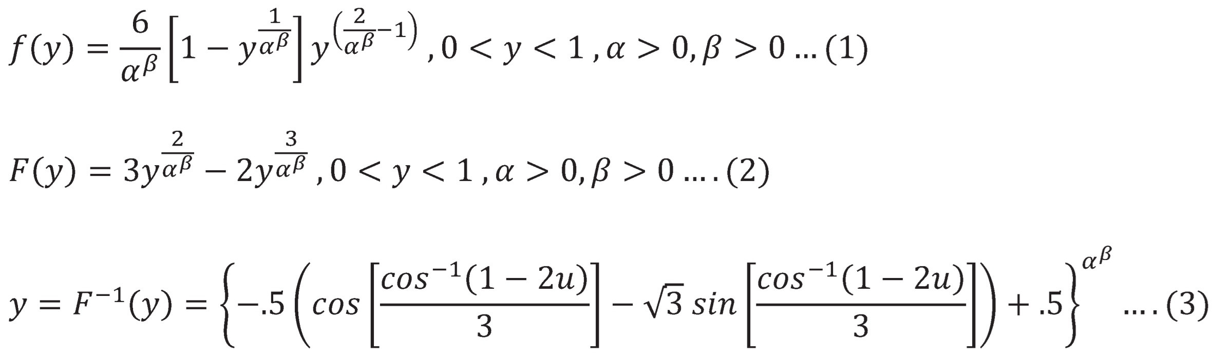
Iman Attia was the first to introduce Median Based Unit Weibull distribution (MBUW)(Iman M.Attia, 2024) (Attia I.M. 2024), given a random variable y distributed as Median Based Unit Weibull distribution (MBUW), the PDF, CDF and quantile functions are as follow:
Various methods are used to estimate the parameters of a distribution. MLE is widely used because it leads to an efficient asymptotically minimum variance though not necessarily unbiased estimator. Methods of moments are ease to apply and obtain. They can be used as starting values for numerical procedures involved in MLE.
(Greenwood et al., 1979) were in favor of Probability weighted moments and initiated the methodology to use it in hydrology for small sample size because the ML does not always work well in small samples. They are leading alternative to MM and MLE for fitting statistical distribution to data, especially distribution written in inverse form; that is, if y is a random variable and F is the value of the CDF for y, the value of y may be written as a function of F; These distributions include the Gumbel, Weibull, and logistic, as well as some less common types, such as, Tukey’s symmetric lambda, Thomas’ Wakeby, and Mielke’s kappa. (Hosking et al., 1985) had advocated PWMs as they demonstrated the outperformance of them over the other estimators using Monte Carlo Simulations. Rather simple expressions for the parameters could be derived for most of these distributions,(J. R. M. Hosking & J. R. Wallis, 1987) including several for which parameters estimates are not readily obtained by using MLE or conventional moments. These distributions are related to many fields like hydrology, resource management and estimation, and forecasting of a number of weather parameter such as temperature, precipitation, wind velocity, flood, drought and rainfall. Many researchers used PWMs like (Ekta Hooda, et al., 2018) for estimating parameters of type II extreme value distribution. (Ashkar F. & Mahdi S., 2003) used the generalized form of PWMs for estimating the two parameter Weibull distribution. (Caeiro & Mateus, 2023) used a new class of generalized PWMs for estimating parameters of Pareto Distribution. (Wang, 1990) used partial PWMs for censored data from generalized extreme value distribution (GEV). Many authors like (Caeiro,F. & Mateus, A., 2017), (Caeiro & Prata Gomes, 2015), (Caeiro et al., 2014), (Caeiro & Ivette Gomes, 2011), (Caeiro & Gomes, 2013), (Rizwan Munir et al., 2013), (Chen et al., 2017), (Vogel et al., 1993) had used PWMs for many distributions mainly the GEV. PWMs are more robust than conventional moments to outliers in the data. PWMs yield more efficient estimators from small data about underlying probability distribution. They are expectations of certain functions of a random variable. So the main advantage over the conventional moment is that they are by definition linear functions of the ordered data and hence suffering less from the effects of sampling variability.
This paper is arranged as follows: section 1 introduces the definition of PWMs and the method of the classic PWMs for parameter estimation. Section 2 derives the PWMs for MBUW and how to use these moments for parameter estimation. Section 3 illustrates the derivation of the asymptotic variance of different estimators. Section 4 discusses the application of this method to real data analysis.
Section 1
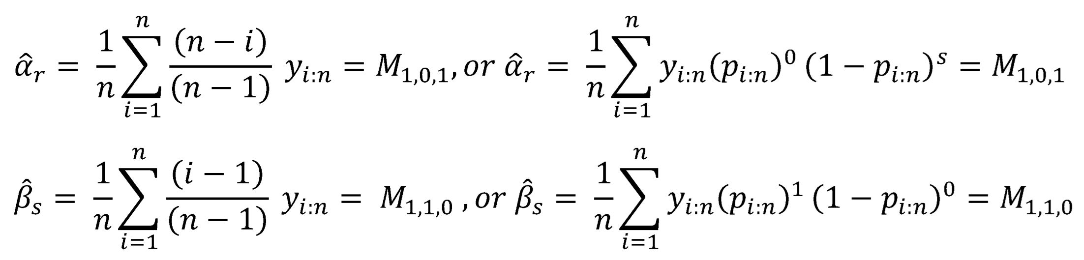
The population PWM is defined as , where are real numbers.
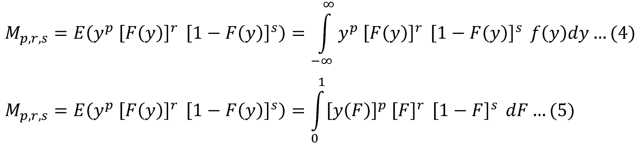
Where is a solution to , in other words, the distribution has a closed form quantile function, inverse CDF.
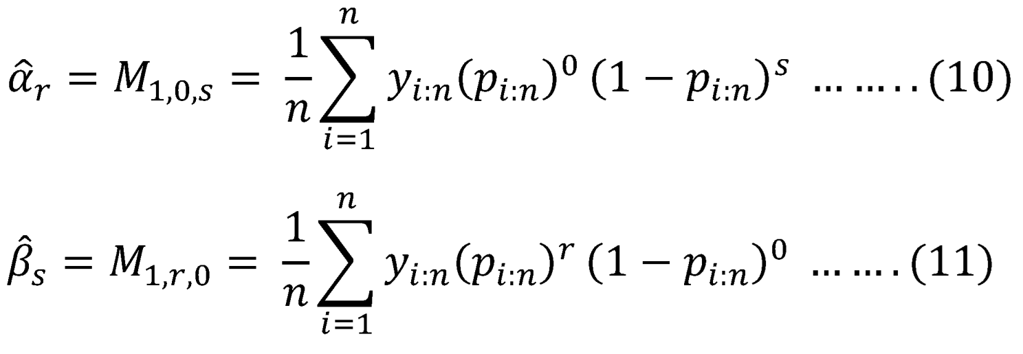
In practice, is chosen to be 1, and so are used for parameter estimation. is the mean. If this mean exists, then exists for any real positive values r and s. They are often restricted to small positive integers values. Choosing has the double advantage of not overweighting sample values unduly and also leads to a class of linear L moments with asymptotic normality (Hosking J.R.M., 1990; Hosking,J.R.M., 1986) Although only small positive integers are required to estimate the parameters of distributions, there is a lot to gain in using real numbers and not necessarily small ones, according to (Rasmussen, 2001) who extended PWMs into generalized PWMs to involve the PWMs with . PWMs is a generalization of classic method of moments when , , are the non-central moments of order p . (Jing, et al. 1989) modified the method to accommodate for the models without an analytic CDF and qunatile function. Greenwood et al. 1979 and Hoskings 1986 advised using because the relations between parameters and moments are much simpler. The empirical estimate of is usually less sensitive to outliers and has good properties when the sample size is small. For convenience, several authors chose to use p=1 and non-negative integer values for r and s. This approach is referred to as the classic PWM method. When p=1, r and s are non-negative , the followings are defined:


Both and are related by the following equations:
For non-negative integers values of r and s that are as small as possible, both and are equivalent. (Landwehr et al., 1979b) defined the sample unbiased estimators for PWMs and as the followings:
The biased estimator is defined as
, so it can be defined for:
Where
(Landwehr et al., 1979a) concluded empirically that moderated biased estimates of the PWMs could produce more accurate estimates of upper quantiles.
In the present paper, and are used as a system of equations to estimate the parameters of the Median Based Unit Weibull (MBUW) distribution. Higher moments and are also used to estimate the parameters and compare the results with lower moments and .
Parameter estimation using PWMs is carried out by equating the analytic expression of the population PWMs by the corresponding sample estimates of PWMs and solving the resulting systems of equations in terms of the parameters.
Section 2: Calculating PWMs for BMUW
2.1. Calculating
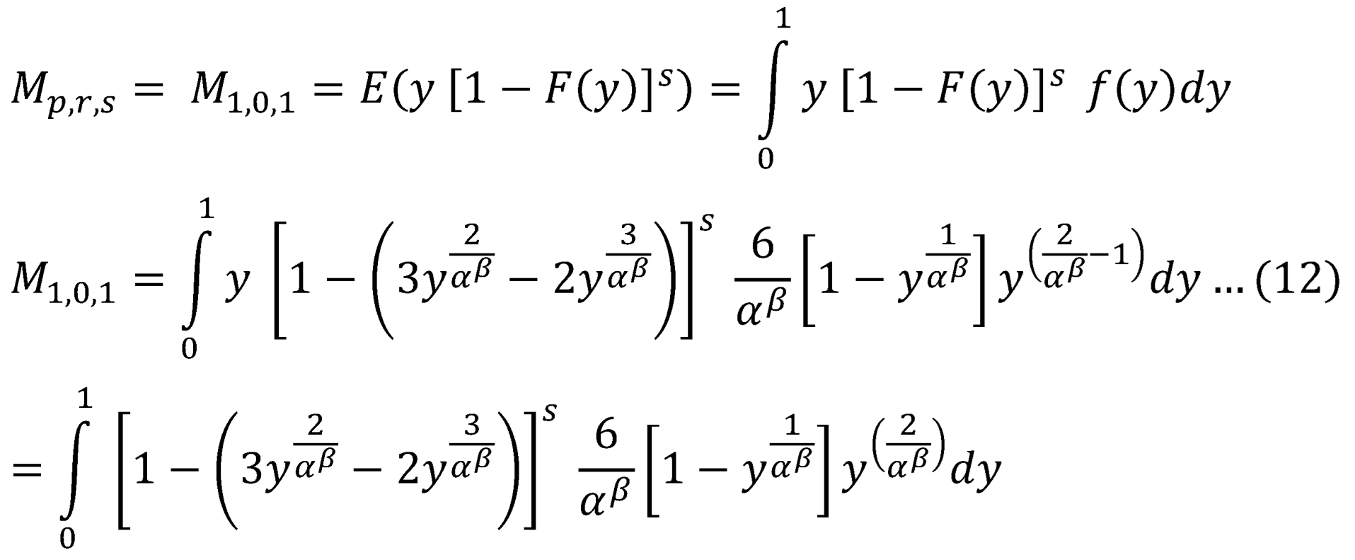
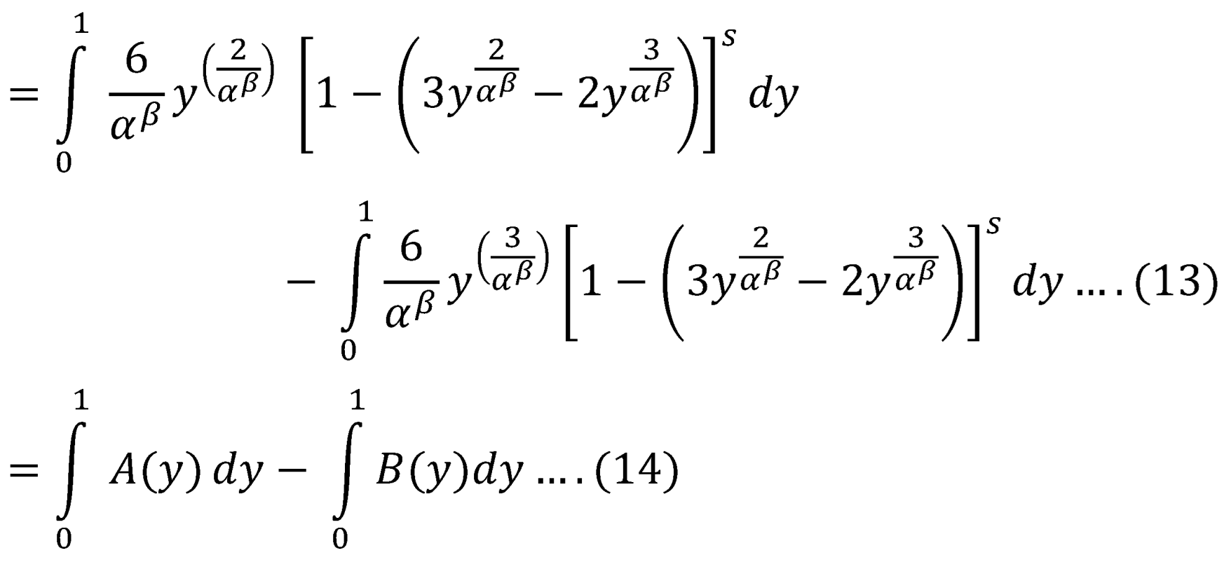
Using binomial expansion in equation (13):
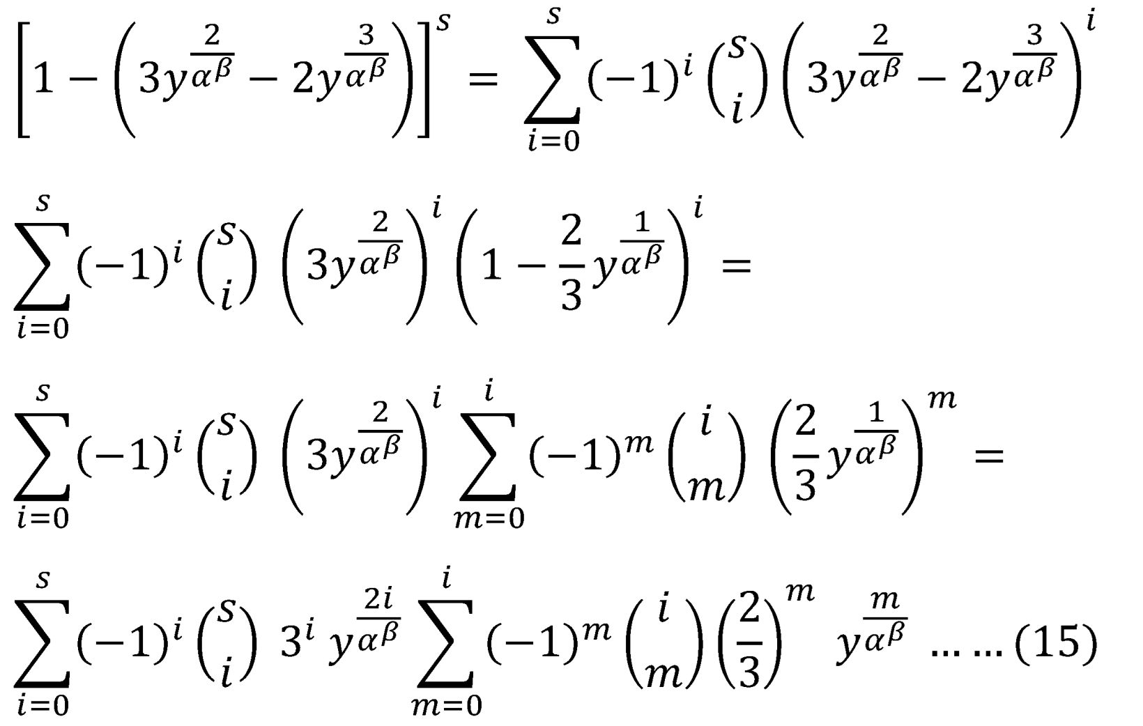
Now exchange integration with summation in equations (13) & (14):
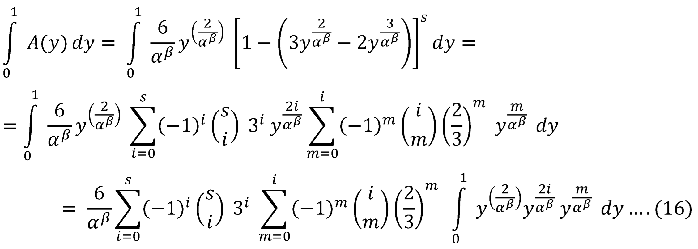
Where the integral is:
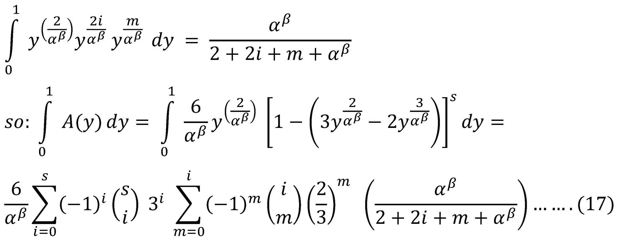
The same steps follow for:
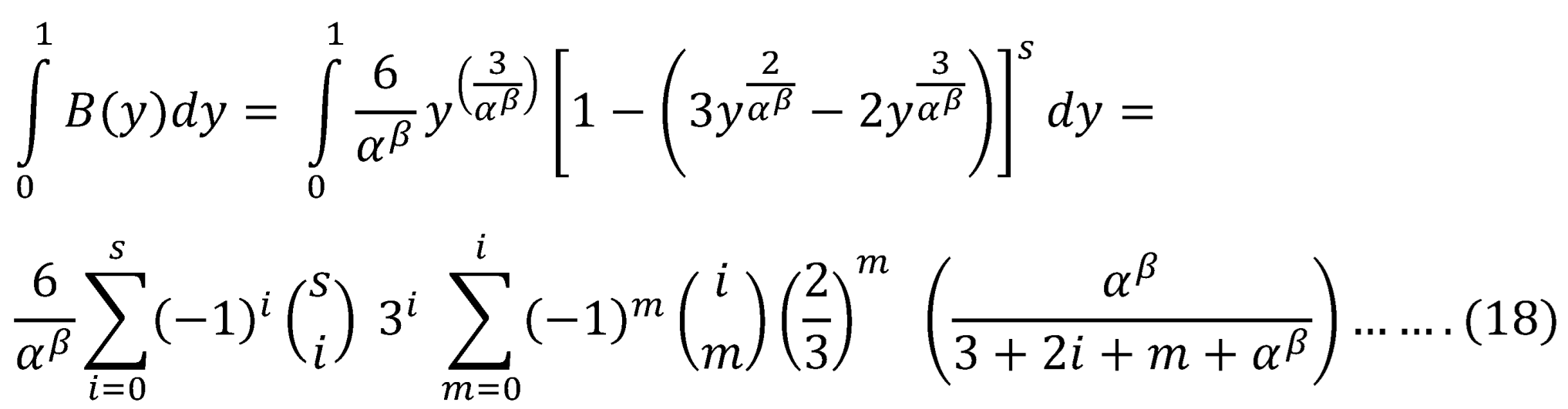
Substitute s=1 in equation (17) and (18):
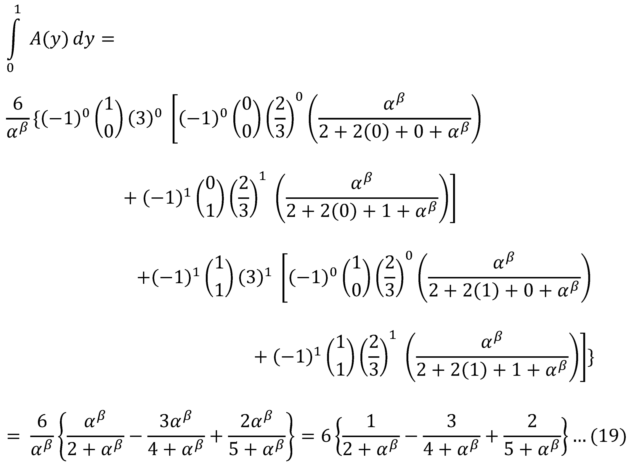
For
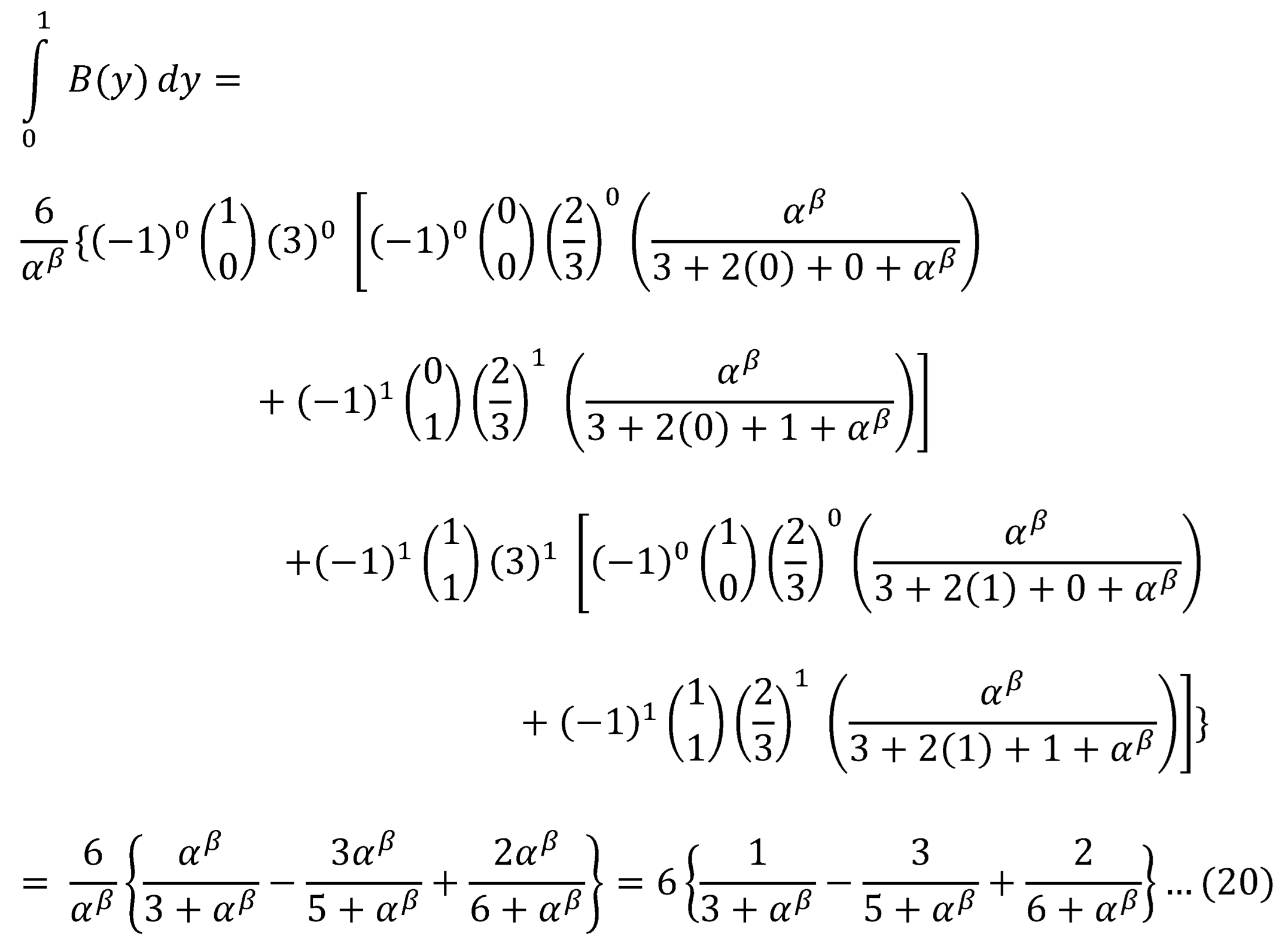
Substitute equation (19) and (20) into equation (14)
2.2. Calculate
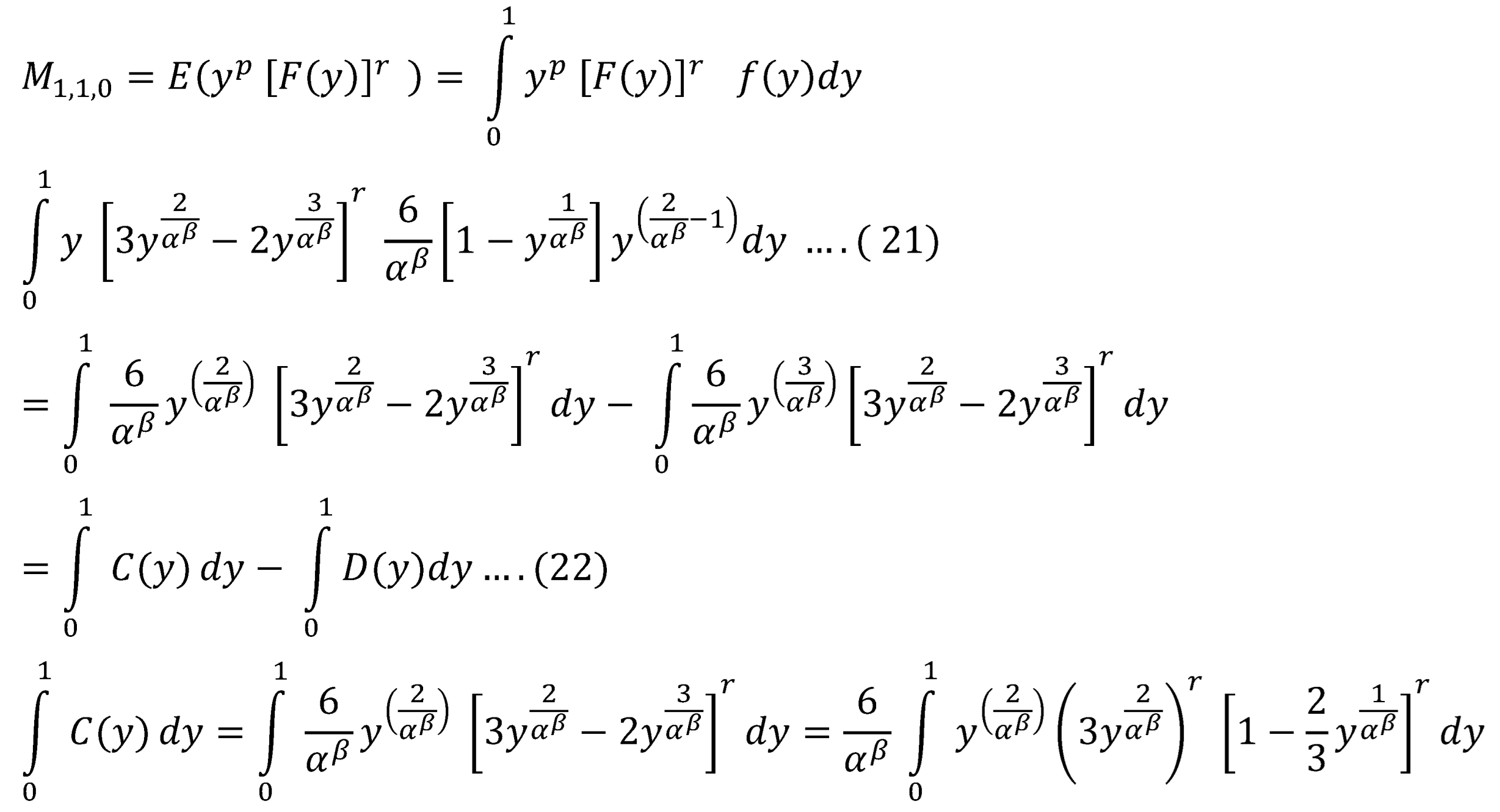
Using binomial expansion:
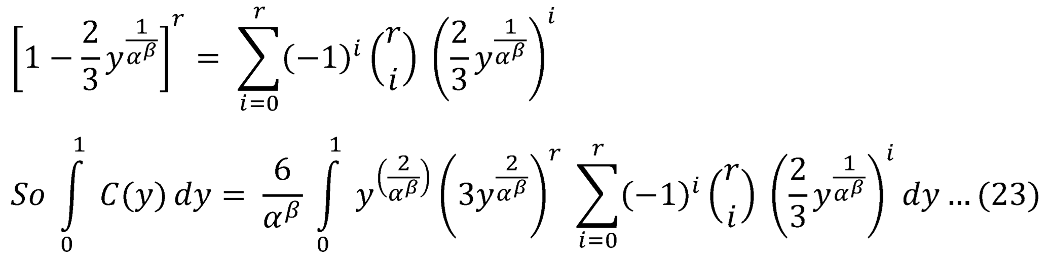
Exchange the integral and the sum
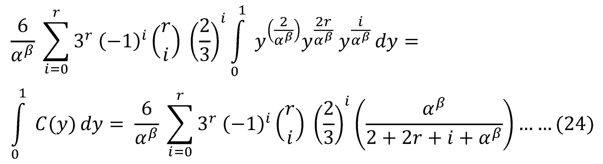
The same steps are followed and give:
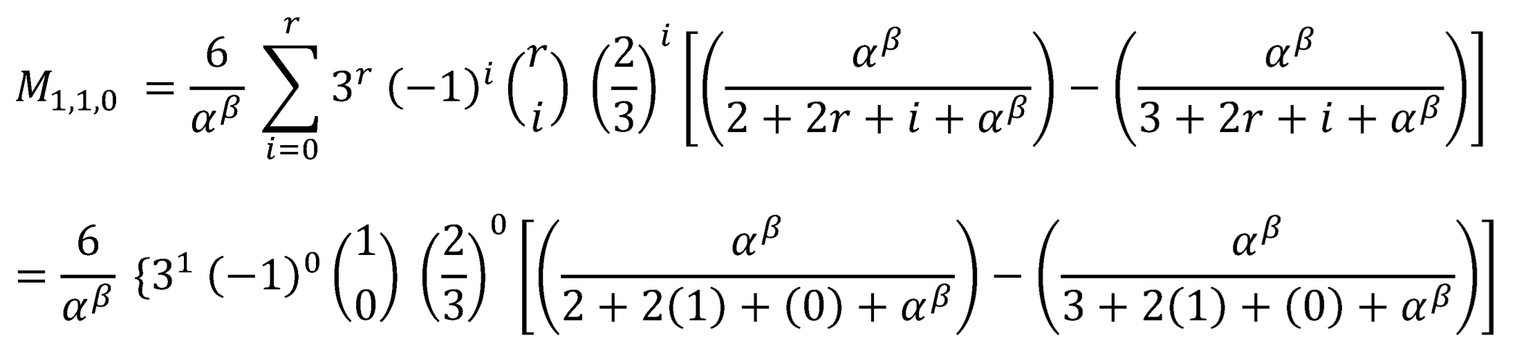
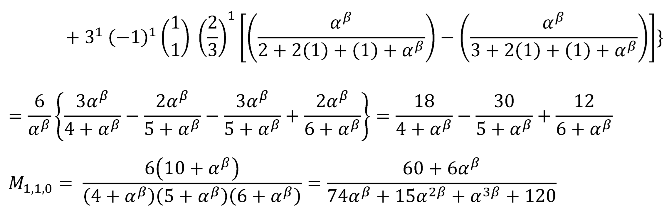
Substitute Equation (24) and Equation (25) into Equation (22) and let r=1
To sum up, PWMs method for estimating the parameters using and :
Step 1: Calculate the population PWMs for the order p=1
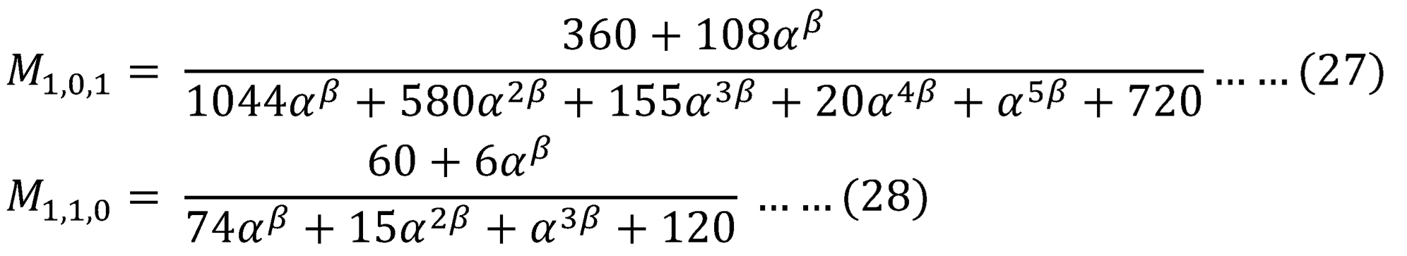
Step 2: Calculate the estimated sample PWMs whether the unbiased or biased estimators and equate these estimators with the corresponding population PWMs.
Step 3: The above equations construct system of equations to be solved numerically. In this paper, the author used Levenberg-Marquardt (LM) algorithm. The objective functions to be minimized are equations (27) and (28).
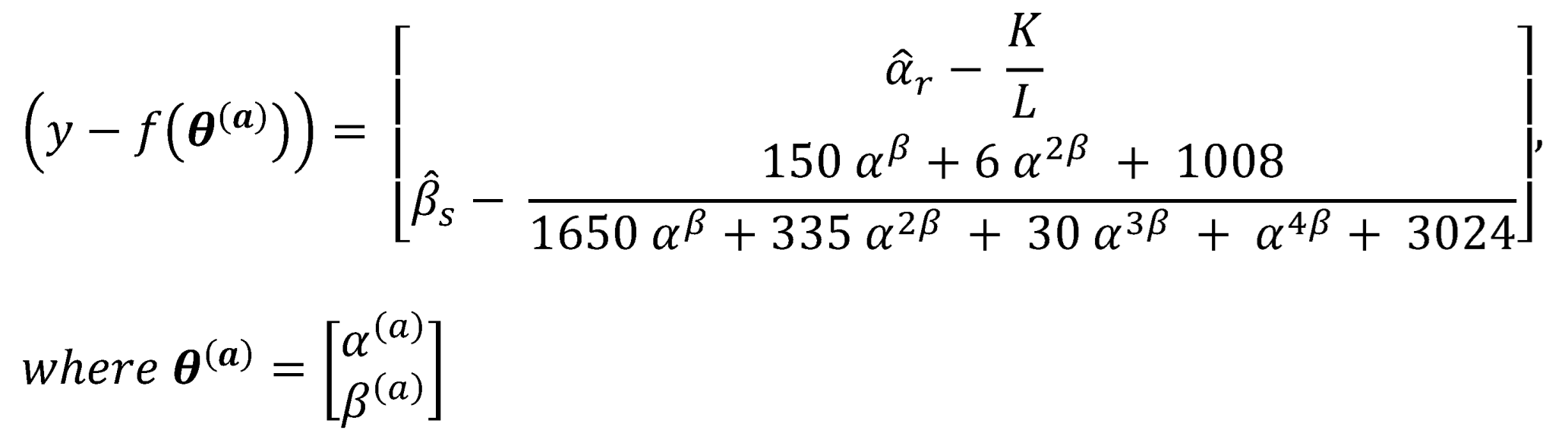
Differentiate the previous equations (27-28) with respect to alpha and beta
The Jacobian matrix is
Apply LM algorithm:
Where the parameters used in the first iteration are the initial guess, then they are updated according to the sum of squares of errors.
LM algorithm is an iterative algorithm.
: this is the Jacobian function which is the first derivative of the objective function evaluated at the initial guess .
is a damping factor that adjusts the step size in each iteration direction, the starting value usually is 0.001 and according to the sum square of errors (SSE) in each iteration this damping factor is adjusted:
: is the objective function (population PWMs, & ) evaluated at the initial guess.
: is the sample estimates of population PWMs , the and .
Steps of the LM algorithm:
- 1-
- Start with the initial guess of parameters (alpha and beta).
- 2-
- Substitute these values in the objective function and the Jacobian.
- 3-
- Choose the damping factor, say lambda=0.001
- 4-
- Substitute in equation (LM equation) to get the new parameters.
- 5-
- Calculate the SSE at these parameters and compare this SSE value with the previous one when using initial parameters to adjust for the damping factor.
- 6-
- Update the damping factor accordingly as previously explained.
- 7-
- Start new iteration with the new parameters and the new updated damping factor, i.e., apply the previous steps many times till convergence is achieved or a pre-specified number of iterations is accomplished.
The value of this quantity: can be considered a good approximation to the variance—covariance matrix of the estimated parameters. Standard errors for the estimated parameters are the square root of the diagonal of the elements in this matrix divided by sample size.
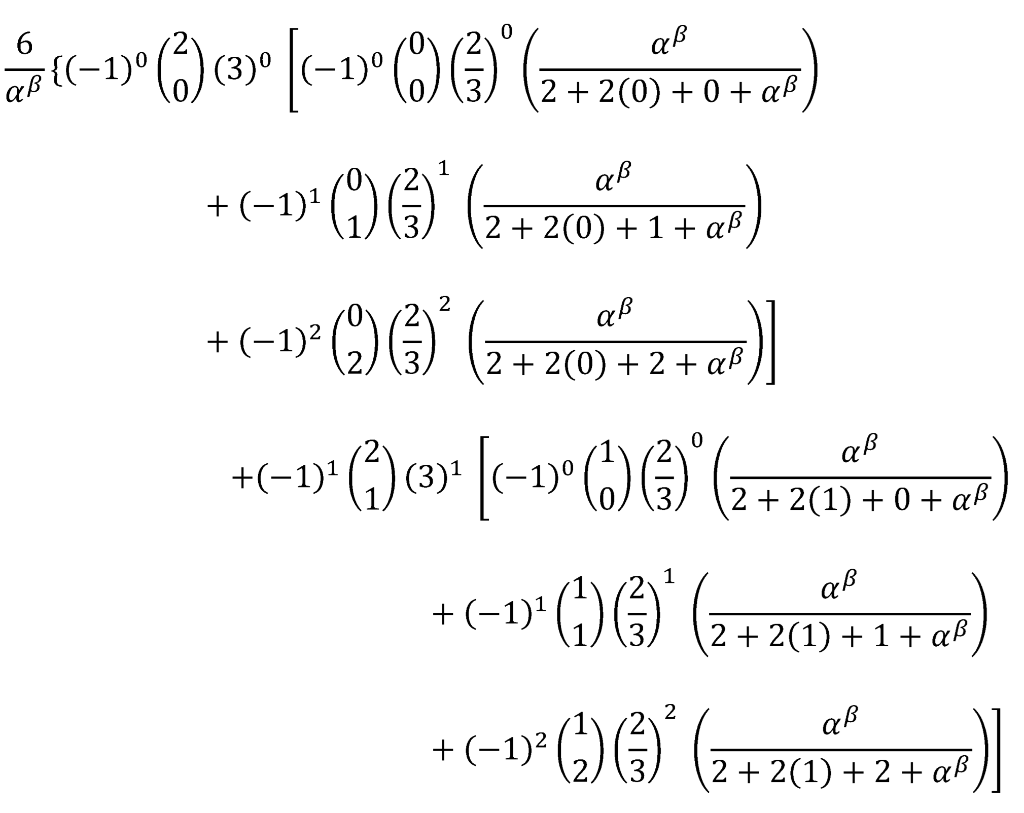
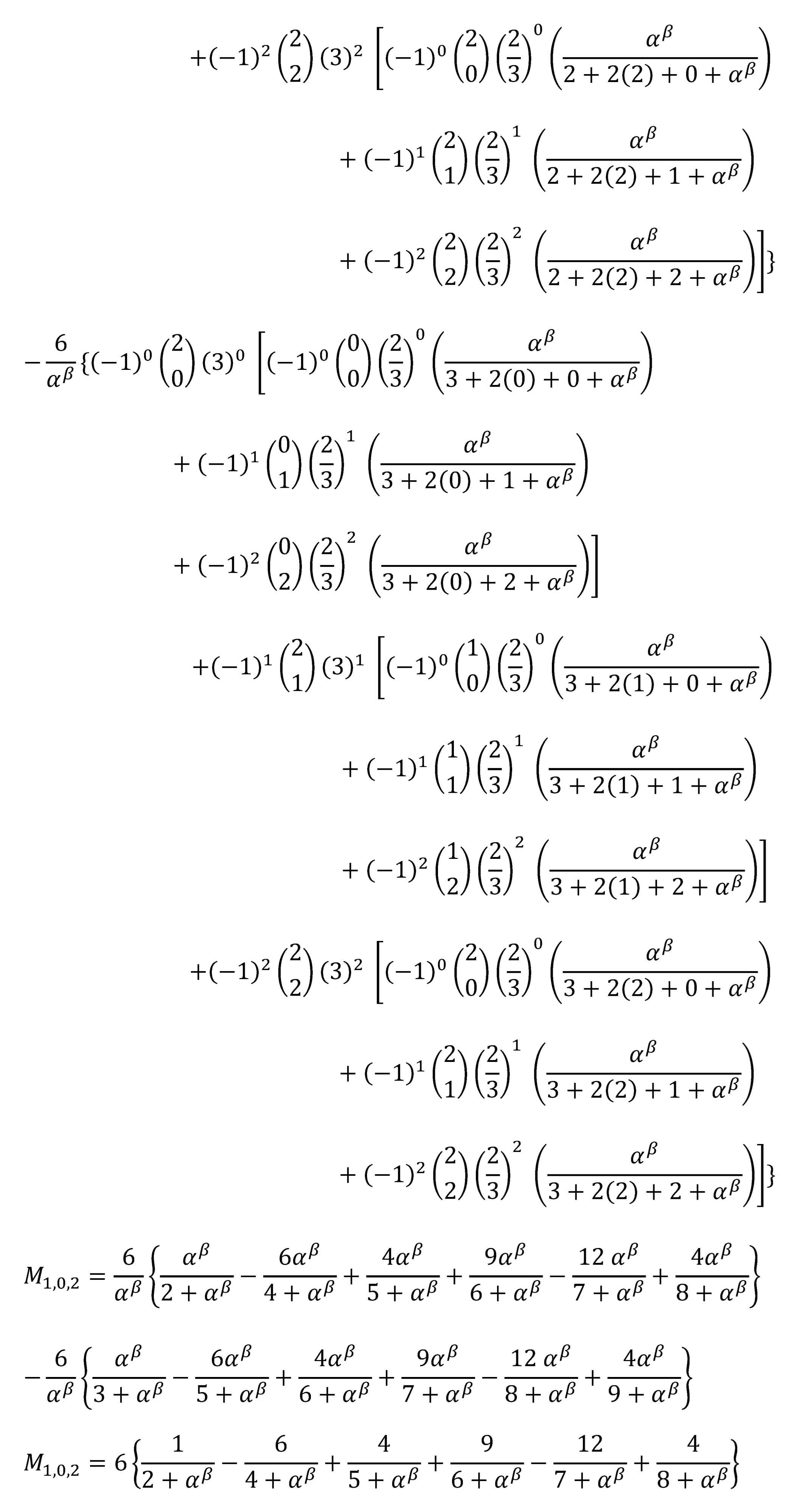
2.3. Calculate
Substitute for s=2 in equation (13) and solve to get:
2.4. Calculate
Substitute for r=2 in Equation (21) and solve to get:
To sum up PWMs method for estimating the parameters using and :
Step 1: Calculate the population PWMs for the order p=1. See equation (29) & (30)
Step 2: Calculate the estimated sample PWMs whether the unbiased or biased estimators and equate these estimators with the corresponding population PWMs.
Step 3: The above equations construct system of equations to be solved numerically. In this paper, the author used Levenberg-Marquardt (LM) algorithm.
The objective functions to be minimized are Equations (29) and (30).
Differentiate the previous Equations (29) and (30) with respect to alpha and beta
The Jacobian matrix is
Apply LM algorithm
Section 3: Asymptotic Distribution of PWM Estimators
Ideally, the comparison of estimators based on different PWMs would be based on analytical expressions for their variances, obtained by asymptotic theory. This would avoid the use of extensive computer simulation. However, in many cases, simple expressions for the asymptotic variance of moments and parameter estimators cannot be found. Moreover, as noted by Hosking1986 and (J. R. M. Hosking & J. R. Wallis, 1987) , asymptotic variance expressions are inaccurate for small samples. Hosking 1986 gave expressions for the asymptotic variances of the generalized pareto parameters estimated using the classical PWMs. The asymptotic variances are a rather inaccurate representation of the true sampling variances when n <50. The asymptotic distribution for the sample PWMs is a linear combination of the order statistics and the results of (Chernoff, et al., 1967) prove that the vector of has asymptotically a multivariate Normal Distribution with mean and covariance matrix . According to (Rao, C.R., 1973) and using the delta method, the covariance matrix has the expression of , where V is the variance of the parameter. The quantity: obtained from applying the LM algorithm for parameters estimation can be considered a good approximation to the variance—covariance matrix of the estimated parameters , the V matrix. The G matrix is the function of the parameter used in the LM algorithm, is the Jacobian matrix.
Section 4: Real Data Analysis
First data: shown in Table 1 ( Flood Data)
This includes 20 observations regarding the maximum flood levels in the Susquehanna River at Harrisburg, Pennsylvania (Dumonceaux & Antle, 1973).
Second data: shown in Table 2 (Time between Failures of Secondary Reactor Pumps)(Maya et al., 2024, 1999)(Suprawhardana and Prayoto)
Descriptive statistics reveals that data has a tail on the right hence exhibiting positive right skewness. The data sets are leptokurtic, exhibiting positive excess kurtosis (kurtosis greater than 3, indicating a fatter tail), as shown in Table 3.
Both data sets show right skewness and positive excess kurtosis (leptokurtic) as shown in Figure 1 and Figure 3.
Table 4 shows the results obtained from applying the LM algorithm to estimate the parameter using PWMs method using the population PWMs in the form of ( with the biased sample estimator for PWMs, compared with the results obtained from using the unbiased sample estimator for the PWMs and the population PWMs in the form of ( . The results are nearly the same. The variance-covariance matrix of estimator obtained by applying the M1,0,1 and M1,1,0 is less than that obtained by applying the M1,0,2 and M1,2,0 although the determinant is the same. The cumbersome computations encountered while applying M1,0,2 and M1,2,0 favors the implementation of M1,0,1 and M1,1,0. The statistical significance of alpha is high. Figure 1 and Figure 2 shows the flood data fitting the MBUW distribution using the PWMs method biased sample PWMs ( and the unbiased sample PWMs ( , respectively. For this data set the unbiased sample estimator used to estimate the higher order PWMs were superior over the biased sampler estimators.
Figure 2.
Shows the flood data fits the MBUW distribution using the PWMs for parameter estimation and the unbiased sample PWMs estimator. (
Figure 2.
Shows the flood data fits the MBUW distribution using the PWMs for parameter estimation and the unbiased sample PWMs estimator. (
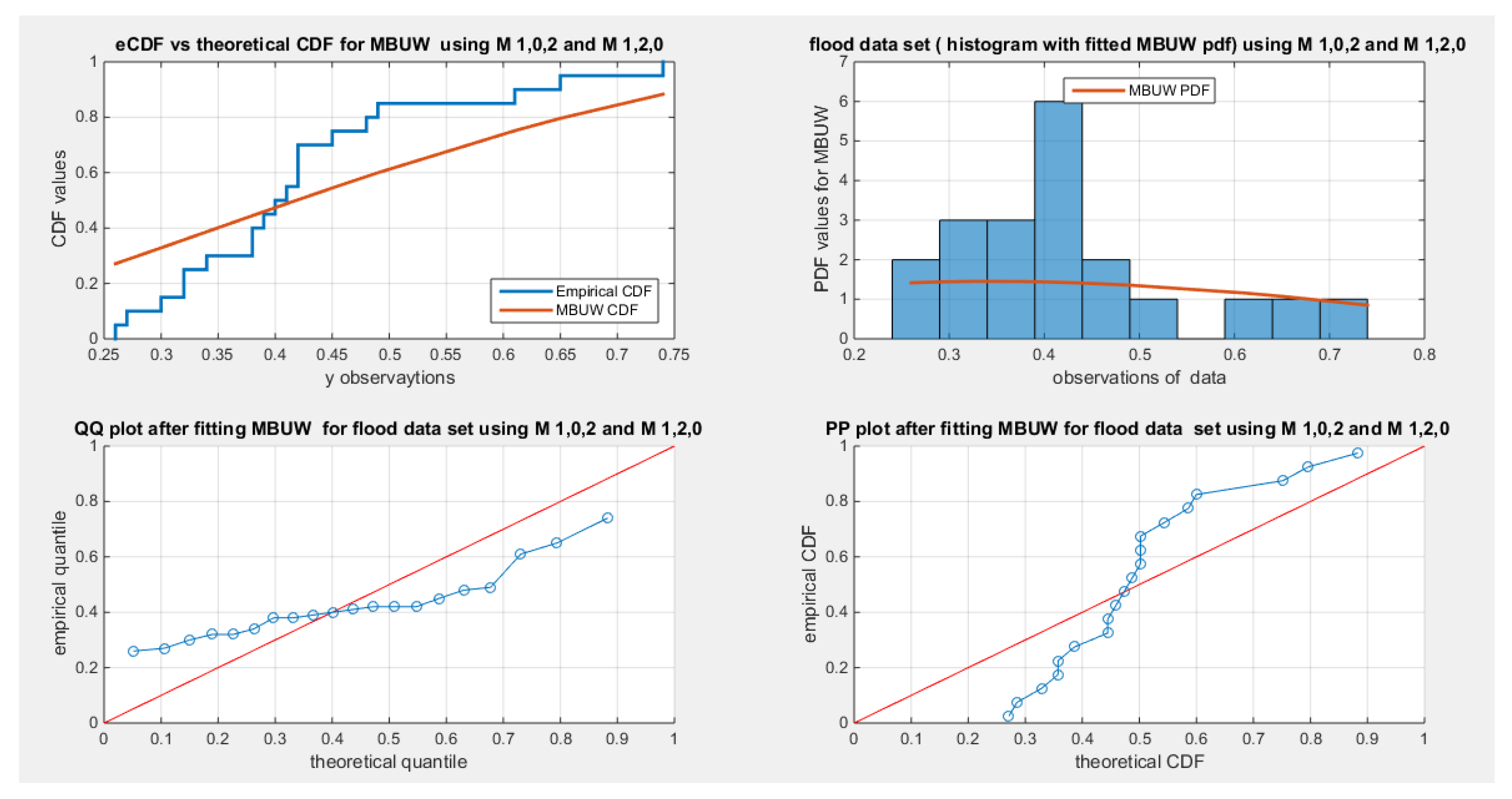
Figure 3.
Shows the flood data fits the MBUW distribution using the PWMs for parameter estimation and the unbiased sample PWMs estimator. (
Figure 3.
Shows the flood data fits the MBUW distribution using the PWMs for parameter estimation and the unbiased sample PWMs estimator. (
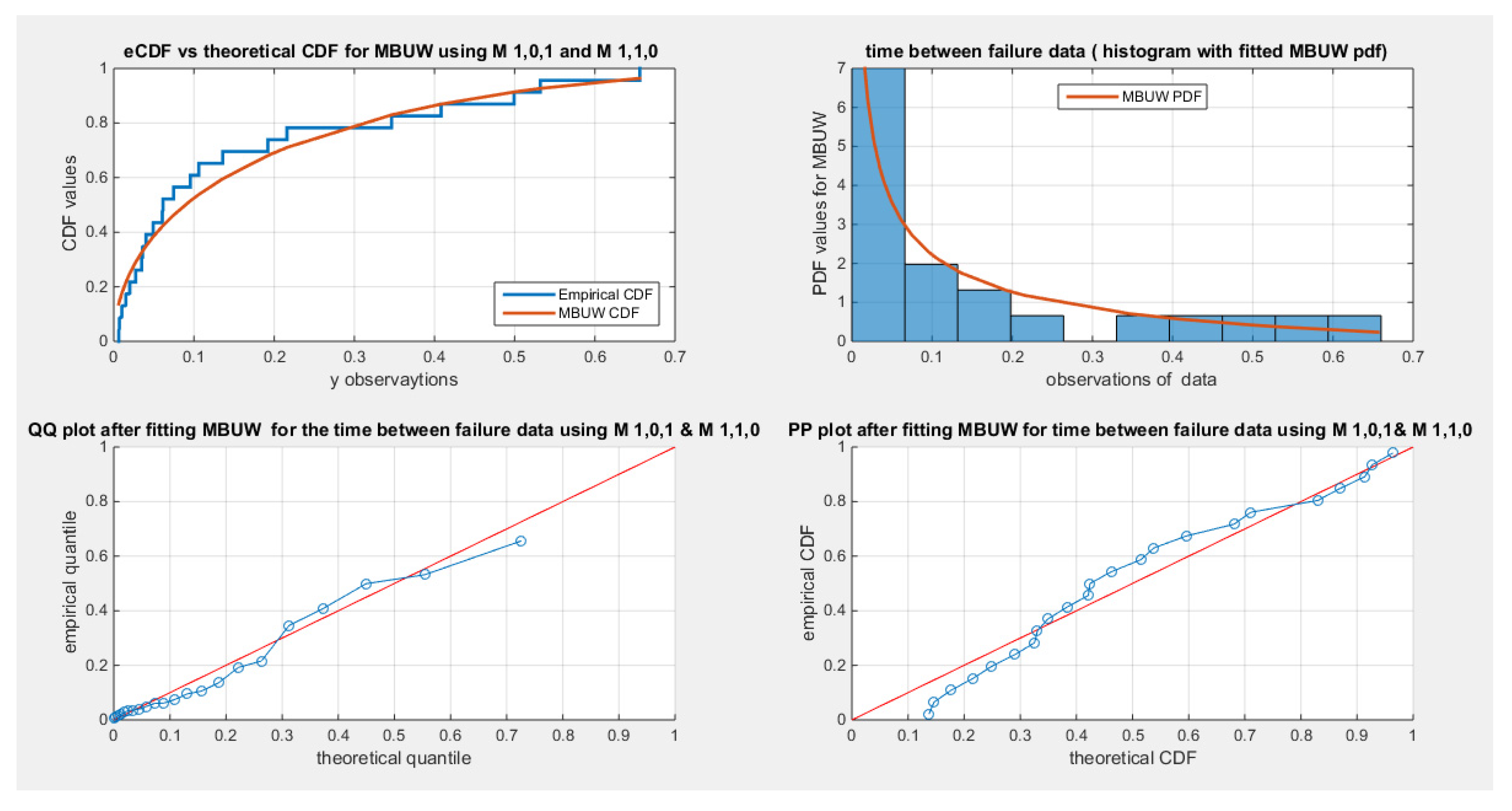
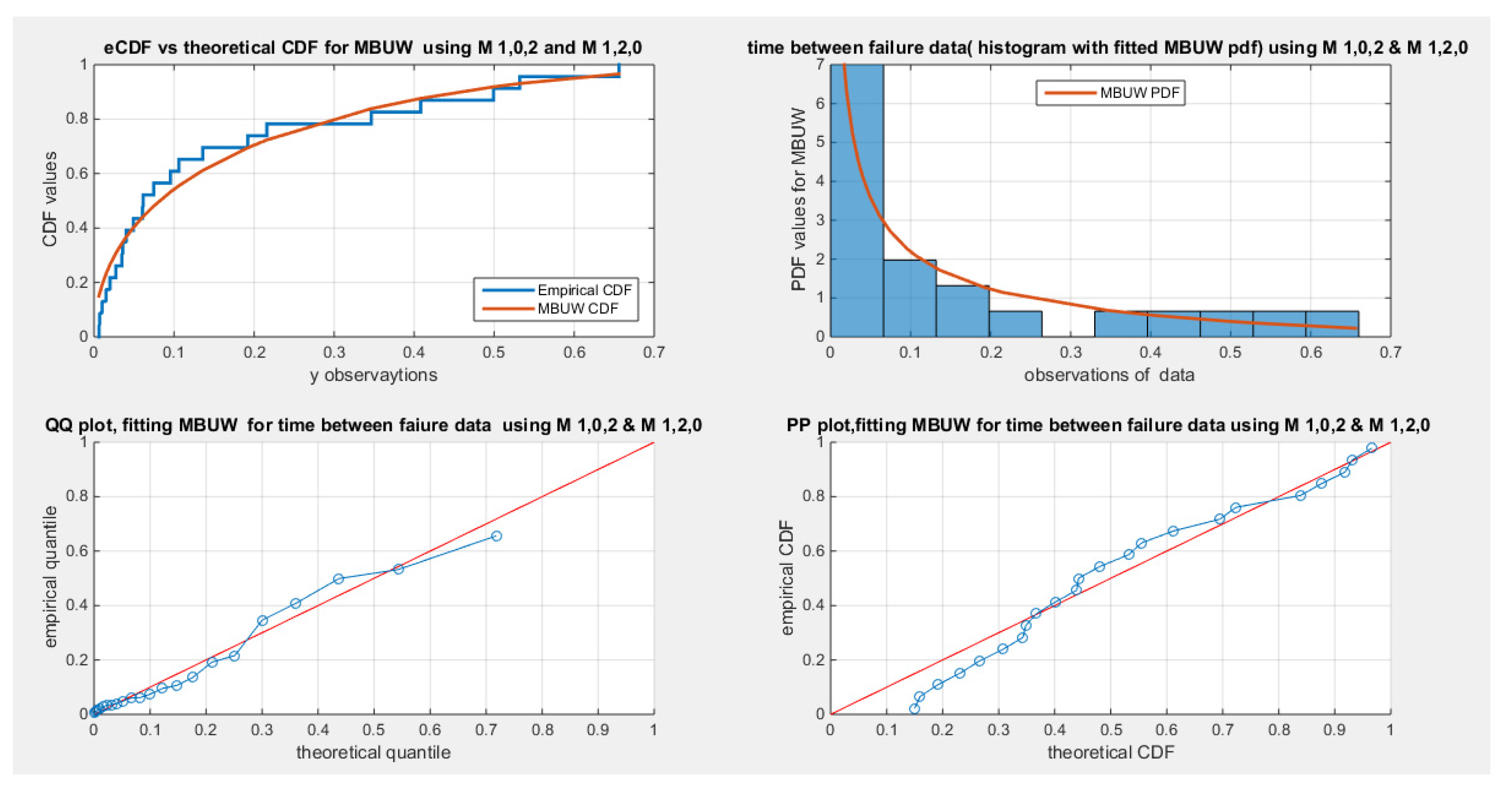
Figure 4.
Shows the flood data fits the MBUW distribution using the PWMs for parameter estimation and the unbiased sample PWMs estimator. (
Figure 4.
Shows the flood data fits the MBUW distribution using the PWMs for parameter estimation and the unbiased sample PWMs estimator. (
Conclusion
The classic PWMs method can be utilized for parameter estimation of the new Median Based unit Weibull (MBUW) distribution. It is robust to outliers. It is simple to obtain than maximum likelihood estimator. The sample estimator for PWM can be either the biased plotting position or the unbiased estimators. For the fitting data set used in this paper, both estimators yielded more or less the same results. The PWMs method has several advantages over other methods of estimation. They are fast and straight forward to compute. They always yield feasible values for the estimated parameters. PWM estimators have asymptotic normal distributions. Higher order moments like did not add much information over the most widely used ones . In this paper the formula used for defining PWM mainly depends on the binomial expansion of the cumulative distribution function and the survival functions. Hence integrating with respect to the variable (dy) rather than integrating with respect to the CDF (dF).
Future work
PWMs are the basis for the L-moment. In the future work, L-moments in different types like L-skewness and L-kurtosis can be estimated and L-moment method can be used for parameter estimation. The beta parameter of the MBUW can be extended to take negative values. For such cases the generalized PWMs (GPWMs) method can be applied. Partial GPWMs can also be applied to censored data.
Author Contributions
AI carried the conceptualization by formulating the goals, and aims of the research article, formal analysis by applying the statistical, mathematical, and computational techniques to synthesize and analyze the hypothetical data, carried the methodology by creating the model, software programming and implementation, supervision, writing, drafting, editing, preparation, and creation of the presenting work.
Funding
No funding resources. No funding roles in the design of the study and collection, analysis, and interpretation of data and in writing the manuscript are declared.
Institutional Review Board Statement
Not applicable.
Informed Consent Statement
Not applicable.
Data Availability Statement
Not applicable. Data sharing does not apply to this article as no datasets were generated or analyzed during the current study.
Acknowledgments
Not applicable.
Conflicts of Interest
The author declares no competing interests of any type.
References
- Ashkar F. & Mahdi S. (2003). Comprison of two fitting methods for the log-logistic distribution. Wter Resources Research, 39(8, 1217), 1–8. [CrossRef]
- Caeiro, F., & Gomes, M. I. (2013). A Class of Semi-parametric Probability Weighted Moment Estimators. In P. E. Oliveira, M. Da Graça Temido, C. Henriques, & M. Vichi (Eds.), Recent Developments in Modeling and Applications in Statistics (pp. 139–147). Springer Berlin Heidelberg. [CrossRef]
- Caeiro, F., Gomes, M. I., & Vandewalle, B. (2014). Semi-Parametric Probability-Weighted Moments Estimation Revisited. Methodology and Computing in Applied Probability, 16(1), 1–29. [CrossRef]
- Caeiro, F., & Ivette Gomes, M. (2011). Semi-parametric tail inference through probability-weighted moments. Journal of Statistical Planning and Inference, 141(2), 937–950. [CrossRef]
- Caeiro, F., & Mateus, A. (2023). A New Class of Generalized Probability-Weighted Moment Estimators for the Pareto Distribution. Mathematics, 11(5), 1076. [CrossRef]
- Caeiro, F., & Prata Gomes, D. (2015). A Log Probability Weighted Moment Estimator of Extreme Quantiles. In C. P. Kitsos, T. A. Oliveira, A. Rigas, & S. Gulati (Eds.), Theory and Practice of Risk Assessment (Vol. 136, pp. 293–303). Springer International Publishing. [CrossRef]
- Caeiro,F. & Mateus, A. (2017). A Log Probability Weighted Moments Method for Pareto distribution. Proceedings of the 17th Applied Stochastic Models and Data Analysis International Conference with 6th Demographics Workshop, pp.211-218.
- Chen, H., Cheng, W., Zhao, J., & Zhao, X. (2017). Parameter estimation for generalized Pareto distribution by generalized probability weighted moment-equations. Communications in Statistics—Simulation and Computation, 46(10), 7761–7776. [CrossRef]
- Chernoff,H., Gastwirth , J.L., & HOHNSjohns, M.V. (1967). Asymptotic distribution of linear combinations of functions of order statistics with applications to estimation. Annals of Mathematical Statistics, 38, 52–72.
- Ekta Hooda, B K Hooda, & Nitin Tanwar. (2018, October). Probability weighted moments (PWMs) and partial probability weighted moments (PPWMs) of type-II extreme value distribution. Conference: National Conference on Mathematics and Its Applications in Science and technologyAt: Department of Mathematics, GJUS&T, Hisar, Haryana, India. Conference: National Conference on Mathematics and Its applications in Science and technologyAt: Department of Mathematics, GJUS&T, Hisar, Haryana, India, India.
- Greenwood, J. A., Landwehr, J. M., Matalas, N. C., & Wallis, J. R. (1979). Probability weighted moments: Definition and relation to parameters of several distributions expressable in inverse form. Water Resources Research, 15(5), 1049–1054. [CrossRef]
- Hosking, J. R. M., Wallis, J. R., & Wood, E. F. (1985). Estimation of the Generalized Extreme-Value Distribution by the Method of Probability-Weighted Moments. Technometrics, 27(3), 251–261. https://www.tandfonline.com/doi/abs/10.1080/00401706.1985.10488049.
- Hosking J.R.M. (1990). L-moment: Analysis and estimation of distributions using ;inear combinations of order statistics. J.R.Statist. Soc, 52(1), 105–124.
- Hosking,J.R.M.,. (1986). The theory of probability weighted moments. Res.Rep,RC12210, IBM ThomasJ. Watson Res. Cent., New York.
- Iman M.Attia. (2024). Median Based Unit Weibull (MBUW): ANew Unit Distribution Properties. 25 October 2024, preprint article, Preprints.org(preprint article, Preprints.org). [CrossRef]
- J. R. M. Hosking & J. R. Wallis. (1987). Parameter and Quantile Estimation for the Generalized Pareto Distribution. TECHNOMETRICS, 29, NO. 3(3), 251–261.
- Jing, D.; Dedun, S.; Ronfu, Y.; Yu, H. (1989). Expressions relating probability weighted moments to parameters of several distributions inexpressible in inverse form. J. Hydrol., 110(J. Hydrol. 1989, 110, 259–270.), 259-270.
- Landwehr, J. M., Matalas, N. C., & Wallis, J. R. (1979a). Estimation of parameters and quantiles of Wakeby Distributions: 1. Known lower bounds. Water Resources Research, 15(6), 1361–1372. [CrossRef]
- Landwehr, J. M., Matalas, N. C., & Wallis, J. R. (1979b). Probability weighted moments compared with some traditional techniques in estimating Gumbel Parameters and quantiles. Water Resources Research, 15(5), 1055–1064. [CrossRef]
- Maya, R., Jodrá, P., Irshad, M. R., & Krishna, A. (2024). The unit Muth distribution: Statistical properties and applications. Ricerche Di Matematica, 73(4), 1843–1866. [CrossRef]
- Rao, C.R. (1973). Linear Statistical Inference and Its Applications (2nd ed.). John Wiley.
- Rasmussen, P. F. (2001). Generalized probability weighted moments: Application to the generalized Pareto Distribution. Water Resources Research, 37(6), 1745–1751. [CrossRef]
- Rizwan Munir, , Muhammad Saleem, , Muhammad Aslam, & and Sajid Ali. (2013). Comparison of different methods of parameters estimation for Pareto Model. Caspian Journal of Applied Sciences Research, 2(1), Pp. 45-56, 2013, 2(1), 45–56.
- suprawhardana. (1999). Suprawhardana, M.S., Prayoto, S.: Total time on test plot analysis for mechanical components of the RSG-GAS reactor. At. Indones. 25(2), 81–90 (1999). 25(2),81-90(1999), 25(5), 81–90.
- Vogel, R. M., McMahon, T. A., & Chiew, F. H. S. (1993). Floodflow frequency model selection in Australia. Journal of Hydrology, 146, 421–449. [CrossRef]
- Wang, Q. J. (1990). Estimation of the GEV distribution from censored samples by method of partial probability weighted moments. Journal of Hydrology, 120(1–4), 103–114. [CrossRef]
Figure 1.
Shows the flood data fits the MBUW distribution using the PWMs for parameter estimation and the biased sample PWMs estimator. (
Figure 1.
Shows the flood data fits the MBUW distribution using the PWMs for parameter estimation and the biased sample PWMs estimator. (
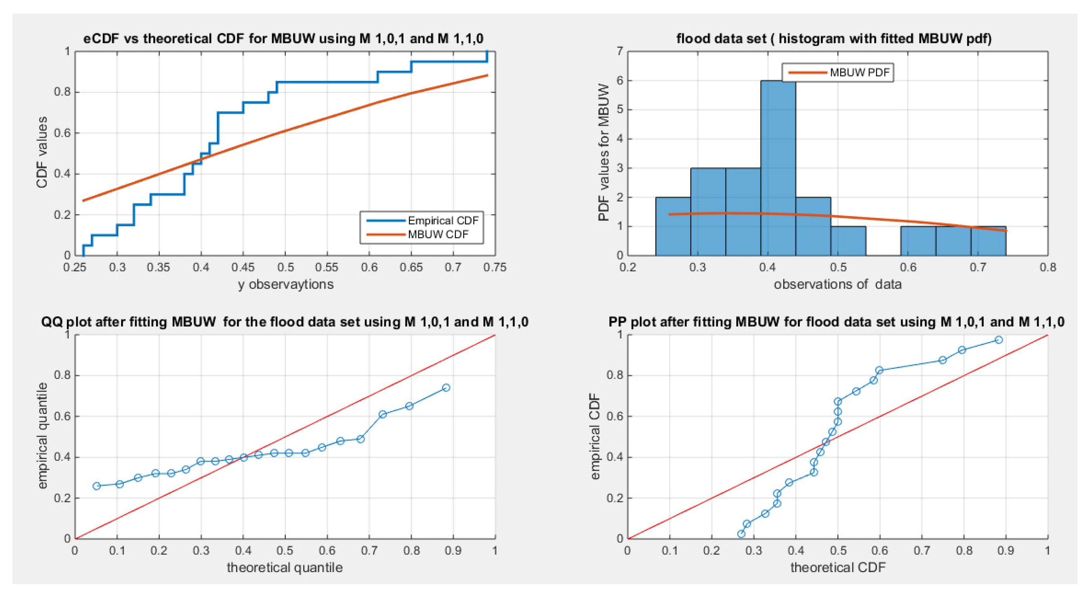

Table 1.
Flood data set.
| 0.26 | 0.27 | 0.3 | 0.32 | 0.32 | 0.34 | 0.38 | 0.38 | 0.39 | 0.4 |
| 0.41 | 0.42 | 0.42 | 0.42 | 0.45 | 0.48 | 0.49 | 0.61 | 0.65 | 0.74 |
Table 2.
time between failures data set.
| 0.216 | 0.015 | 0.4082 | 0.0746 | 0.0358 | 0.0199 | 0.0402 | 0.0101 | 0.0605 |
| 0.0954 | 0.1359 | 0.0273 | 0.0491 | 0.3465 | 0.007 | 0.656 | 0.106 | 0.0062 |
| 0.4992 | 0.0614 | 0.532 | 0.0347 | 0.1921 |
Table 3.
descriptive statistics of flood data and time between failures:.
| min | mean | St.dev. | skewness | kurtosis | Q(1/4) | Q(1/2) | Q(3/4) | max | |
| Flood data |
0.26 | 0.4225 | 0.1244 | 1.1625 | 4.2363 | 0.33 | 0.405 | 0.465 | 0.74 |
| Time Bet- failure |
0.0062 | 0.1578 | 0.1931 | 1.4614 | 3.9988 | 0.0292 | 0.0614 | 0.21 | 0.656 |
Table 4.
comparisons of the results of PWMs method for parameter estimation of flood dataset using and
Table 4.
comparisons of the results of PWMs method for parameter estimation of flood dataset using and
| thetas | alpha | 1.1898 | 1.222 | |||
| beta | 1.2983 | 1.1393 | ||||
| Var-cov matrix of parameter |
54.3338 | -225.5809 | 101.3959 | -193.1974 | ||
| -225.5809 | 946.1895 | -193.1974 | 954.4631 | |||
| AD | 2.4549 | 2.457 | ||||
| CVM | 0.4449 | 0.4453 | ||||
| KS | 0.2517 | 0.2504 | ||||
| H0 | Fail to reject | Fail to reject | ||||
| P-KS test | 0.0889 | 0.0862 | ||||
| SSE | 0.0558 | 0.0021 | ||||
| , unbiased estimator | - | 0.1096 | ||||
| , unbiased estimator | - | 0.1774 | ||||
| Pi, biased estimator | 0.37 | - | ||||
| Pi complementary | 0.37 | - | ||||
| Sig_a | 209.77 (p<0.001) | 33.711(p,0.001) | ||||
| Sig_b | 26..1412 (p<0.001) | 35.3896 (p<0.001) | ||||
| Variance Estimator, after delta method application. |
0.0006 | 0.0056 | 0.0263 | 0.0233 | ||
| 0.0056 | 0.0493 | 0.0233 | 0.0207 | |||
| Det. of var. estimator |
0 | 0 | ||||
| Trace of var. estimator |
0.05 | 0.0494 | ||||
Table 5.
comparisons of the results of PWMs method for parameter estimation of time between failures dataset using and
Table 5.
comparisons of the results of PWMs method for parameter estimation of time between failures dataset using and
| thetas | alpha | 2.0138 | 2.0381 | |||
| beta | 1.7844 | 1.8023 | ||||
| Var-cov matrix of parameter |
383.295 | -485.9643 | 436.5251 | -453.6834 | ||
| -485.9643 | 617.0596 | -453.6834 | 634.7154 | |||
| AD | 0.5520 | 0.5925 | ||||
| CVM | 0.0799 | 0.0808 | ||||
| KS | 0.1141 | 0.1066 | ||||
| H0 | Fail to reject | Fail to reject | ||||
| P-KS test | 0.7282 | 0.625 | ||||
| SSE | 0.0000058 | 0.00000026 | ||||
| , unbiased estimator | 0.0298 | 0.0110 | ||||
| , unbiased estimator | 0.1280 | 0.1092 | ||||
| Pi, biased estimator | - | - | ||||
| Pi complementary | - | - | ||||
| Sig_a | 1246.77 (p<0.001) | 171.5518 (p,0.001) | ||||
| Sig_b | 39.5574 (p<0.001) | 44.8539 (p<0.001) | ||||
| Variance Estimator, after delta method application |
0.0001 | 0.0019 | 0.0032 | 0.011 | ||
| 0.0019 | 0.0434 | 0.011 | 0.0371 | |||
| Det. of var. estimator |
0 | 0 | ||||
| Trace of var. estimator |
0.0435 | 0.0404 | ||||
Disclaimer/Publisher’s Note: The statements, opinions and data contained in all publications are solely those of the individual author(s) and contributor(s) and not of MDPI and/or the editor(s). MDPI and/or the editor(s) disclaim responsibility for any injury to people or property resulting from any ideas, methods, instructions or products referred to in the content. |
© 2025 by the authors. Licensee MDPI, Basel, Switzerland. This article is an open access article distributed under the terms and conditions of the Creative Commons Attribution (CC BY) license (http://creativecommons.org/licenses/by/4.0/).
Copyright: This open access article is published under a Creative Commons CC BY 4.0 license, which permit the free download, distribution, and reuse, provided that the author and preprint are cited in any reuse.


