
Submitted:
10 December 2024
Posted:
10 December 2024
You are already at the latest version
Abstract
Because of its location at the meeting point of the Eurasian Plate and the Philippine Sea Plate, Taiwan experiences earthquakes frequently. Mountains and hills make up the majority of the landscape, and Taiwan has some of the highest precipitation levels in the world. The stability of slopes in different parts of Taiwan is influenced by all of these factors. The study's instances are the National Freeway 1 and 5 slopes, where several landslide and rockfall incidents have occurred. This study used PLAXIS 2D CE finite element software to simulate and analyze the safety of highway slope protection projects. Displacements induced by normal and high groundwater levels were discussed. Moreover, a pseudo-static study of slope displacements under seismic conditions was performed. According to the results of the numerical study, the force operating on the slope was centered on the sliding surface when the groundwater level was normal, and it extended to the top when the groundwater level was high. By comparison, under seismic conditions, the force acting on the slope extended to the whole slope.
Keywords:
slope
; slope protection engineering
; groundwater level
; finite element
; pseudo-static analysis
1. Introduction
Many nations have constructed substantial road networks and residential communities in hilly and mountainous terrain as a result of global population increase and socioeconomic development. But occasionally, landslides happen, and they can be extremely dangerous for people and property, particularly in places with steep terrain and a lot of rainfall [1,2,3]. Thus, geotechnical researchers have focused increasingly on slope stability assessment [4,5,6,7,8,9,10,11,12,13,14,15,16].
In mountainous regions, landslides rank among the most dangerous natural calamities [17,18]. Taiwan's landscape is primarily made up of hills and mountains, which make up almost two-thirds of the island's overall area. As a result, safety in the event of landslides is a major concern for the appropriate government bodies. Since the construction of National Freeway 1, the demand for motorways has grown. The freeway segment between Keelung and Xizhi was constructed 46 years ago, and shotcrete has been used to cover the bedrock slope's surface. The shotcrete covering has been repaired and maintained, but aging has led to cracks and plant growth on the surface. It is worth noting that on National Freeway 5, several slopes are classified as high-risk according to the technical specifications of the Freeway Maintenance Manual of the Freeway Bureau of the Ministry of Transportation and Communications of the Republic of China in Taiwan.
The southbound exits at Wudu on National Freeways 1 and 5 with high-risk slopes were chosen as case studies in light of the aforementioned. Numerous landslides have occurred close to these locations. Slope displacement at normal and high groundwater levels was simulated using the PLAXIS 2D CE finite element analysis tool, and variations in acceleration, speed, and displacement in slope models were examined using pseudo-static analysis in seismic circumstances. In the future, the numerical simulation results might be helpful for preventing the collapse of roadway slopes when severe rains or other conditions impair their stability.
2. Literature review
2.1. Slope Stability
Under specific geological background circumstances, slope instability typically arises as a result of the excitation of initiating events like intense earthquakes and heavy rains [19]. A hillslope's stability can be affected by a variety of causes. Geological material, geological structure, topographic and environmental conditions, and engineering considerations are the four main causes of landslides, according to Hung [20].
- Geological material: The slope stratum is mainly composed of single or multiple geological materials. The cementation, particle size, and composition of the geological materials will directly affect the stability of the slope.
- Geological structure: In geological structures, the orientation of weak planes (such as strike and dip angle) and the type of slope (such as dip slope, escarpment, and oblique slope) are crucial characteristics. Slope stability is compromised by other geological features that split slopes into discontinuous or fragmented rocks, such as bedding surfaces, joints, folds, faults, and other discontinuities. This reduces the strength of the rock mass and increases weathering.
- Environmental and topographic factors: Topography includes the slope's general form and rough surface terrain. While slope terrain has its own height and gradient, surface terrain relates to the characteristics of the geological structure. Groundwater, earthquakes, and rainfall are examples of environmental elements that affect slope stability.
- Engineering aspects: Slope stability is affected directly or indirectly by human factors such as highways, tunnel excavation, blasting, overdevelopment of slopes, bad building or site selection, poor slope drainage systems, inadequate maintenance of protective structures, etc.
In Taiwan, accidents involving slopes are common in building projects. Slope patrol, slope monitoring, and ground anchor inspection are used to keep an eye on stability in order to prevent collapse due to the sudden failure of rock or soil mass on a slope. To increase the facilities' service life, slope safety evaluation and categorization are also done. To put it briefly, these facilities' preventive maintenance lowers the chance of failure and averts catastrophes. Slopes are divided into four classes—A, B, C, and D—per the Freeway Maintenance Manual. The following is a description of the classification criteria and remedies:
- Class A slope: Instability is obviously present. Increased patrols and observation are necessary, as is prompt intervention.
- Class B slope: Due to the possible indication of instability, additional patrols, monitoring, maintenance, reinforcing, and remediation are needed.
- Class C slope: It needs regular patrol or maintenance, with monitoring as necessary, even if there are no obvious signs of instability.
- Class D slope: Patrolling is still necessary even though it is steady.
2.2. Prediction of Slope Stability
Predicting slope stability has been the subject of numerous studies over the last few decades. These research' methodologies can be broadly categorized into three groups: finite element technique (FEM), limit equilibrium method (LEM), and limit analysis method (LAM) [21]. Due to its ease of use, the LEM is one of the most popular approaches among them [22]. However, several idealized assumptions about the LEM make its response imprecise. Because it puts strict restrictions on limit state solutions [23] and offers a straightforward calculation procedure, the LAM is commonly used in slope stability [24]. However, when dealing with complicated slope structures and variable soil deposition, it can be difficult to create theoretical formulations of upper or lower bounds [21].
Compared to the LEM and LAM, the FEM appears to be a more reliable and adaptable processing technique for slope performance modeling and evaluation [21,25,26,27]. Kafle et al. [7] constructed a finite element model to simulate the Bianjiazhai landslide near the Suofengying reservoir at the Wu River in Guizhou Province, China. Their results showed that sudden reservoir level fluctuations had a critical effect on the stability of the slope. In addition, a strength reduction analysis confirmed that the deformation behavior of the slope was mainly a shear-slip phenomenon, and the associated shear zones were identified. In order to accurately and efficiently simulate in situ stress prior to seismic loading, Kontoe et al. [28] used pseudo-static finite element analysis. They also investigated how sensitive the analysis findings were to the finite element mesh level.
The main metric used to assess slope stability is the safety factor [10], which is the ratio of the available shear strength to the equilibrium shear stress along a specific failure surface [4]. Assumptions on the form and location of the failure surface are not required when utilizing the FEM for a slope stability analysis. According to the FEM, failure occurs when the soil's shear strength is not strong enough to support the sliding force of the slope, and it is feasible to model how displacement and slope failure will develop. The FEM often employs the soil shear strength reduction technique to calculate the slope's safety factor [29]. During the slope failure process, soil cohesion c and internal friction angle φ continue to decrease. According to the literature, no matter how the slope is formed, when it reaches the failure state, the reduced cohesion tends to have the same value. Accordingly, Zienkiewicz et al. [30] reduced the strength parameters (c, tanφ) of a slope step-by-step through a reduction factor of 1/N, and the reductions for the two parameters were equal. When reduced to the failure state, the N value at this time can be defined as the safety factor of the slope.
Using the region close to the top of the neighboring slope toe as the chosen node, Giam and Donald [31] calculated the slope's overall safety factor by examining the link between the node displacement and the change in soil strength characteristics (cohesion and friction angle). Ugai [32] determined the system's overall safety factor iteratively by adopting a minimal system safety factor value for the material's strength (c and φ). To determine whether the system is unstable, they then performed finite element analysis using the converted material strength. Brinkgreve and Bakker [33] used the PLAXIS finite element formula they developed to calculate the slope's safety factor and the corresponding failure sliding surface position in addition to the shear strength reduction technique. The idea of shear strength reduction was used by Matsui and San [34] to assess slope safety factors and the emergence of possible slip surface failure. Additionally, the shear strain in the failure process that extends from the slope's base to its summit (i.e., total shear failure) was classified as slope failure. Ugai and Leshchinsky [35] extended the two-dimensional problem to three dimensions. They used 20-node isoparametric solid elements and reduced integration with 8 Gaussian integration points to conduct a three-dimensional vertical excavation slope simulation, taking into account the influence of pseudo-static seismic forces. The analysis results are compared with the results of the limit equilibrium method to verify their rationality. Griffiths and Lane [36] used the FEM to apply shear strength reduction to the analysis of slope stability, taking into account the effects of weak interlayers in the soil and groundwater. The occurrence of slope failure was determined by the non-convergence of the solution, because slope failure is often accompanied by a rapid increase in displacement. The position and shape of the critical slip surface were represented by a deformed mesh diagram and node displacement vector diagram. In addition, the analysis results of the safety factor were compared with those of the limit equilibrium method. Based on the incremental method of elastic–plastic mechanics and the bilinear projection operator, Sun et al. [29] combined the strength reduction method with the φ-ν inequality and proposed a virtual element strength reduction method for slope stability analysis. The deformation of homogeneous and heterogeneous slopes under different strength reduction coefficients was solved, and the grid dependence of this method was discussed. Furthermore, numerical examples were used to verify the correctness and effectiveness of the proposed method.
2.3. Pseudo-Static Analysis of Soil Inertial Force
One of the primary dynamic loads frequently observed on soil or rock slopes is seismic force [19]. Rock or soil slopes are subject to enormous dynamic stress, which has a significant impact on their stability. The pseudo-static analysis based on force equilibrium assumes that seismic force is a static inertial force operating laterally on the structure while assessing structural stability. Throughout the analysis, the seismic coefficient was progressively raised. To ascertain the seismic load that the structure can withstand as it approaches critical stability, a number of stability analyses were conducted.
The limit equilibrium approach, also known as the Mononobe–Okabe (M-O) method, was created in Japan in the 1920s by Okabe [37] and Mononobe and Matsuo [38]. It serves as the foundation for the most widely used cantilever and gravity structure analysis. For pseudo-static analysis, the M-O approach is also frequently employed. It calculates the dynamic soil pressure coefficient based on force equilibrium after transforming the seismic load into the inertial force of soil mass. Dynamic soil pressure, or active soil pressure under dynamic conditions, is depicted in equation (1). Figure 1a displays the stresses produced under dynamic conditions, while Figure 1b displays the stress path produced by the soil mass's inertial force under static conditions.
In Equation (1), KV is the vertical seismic coefficient, KAE is the dynamic soil pressure coefficient, is the unit weight of soil, and H is the wall height. Various modifications of the M-O method have been introduced. Seed and Whitman [39] separated dynamic soil pressure (PAE) into static soil pressure (PA) and seismically induced soil pressure (ΔPdyn), as shown in Equation (2):
3. Overview of the Case Studied
For this investigation, three locations were selected. Site 1 may be found at the Freeway 1 Wudu exit (Figure 2), while Site 2 is situated at Freeway 5 with a 7K+082 mileage (Figure 3), and Site 3 is situated at Freeway 5 with a 7K+410. The geological data and the overview of the slope protection project for each site are described below, and they act as a guide for the input values utilized in the subsequent numerical analysis.
According to the geological maps supplied by Taiwan's Central Geological Survey, the stratum at Site 1 is the Nangang Formation, which is made up of thick layers of dark shale and slate-gray tuffaceous sandstone. The slope is protected by RC curtain walls, free-styled grill beams, and grouted anchor bars. The grouted anchor bars are composed of three-meter-long #8 steel bars spaced three meters apart horizontally.
The Nangang Formation, the stratum at Site 2, is interlayered with sandstone and shale and is located 4.9 meters below the colluvium's ground surface. A total of 26 layers of 30 tons of prestressed ground anchors are used to protect the slope. The current ground anchors consist of a fourth-stage, 15-layer ground anchor; a free section of five meters; an anchor section of five meters; and a horizontal spacing of three meters. After that, eleven levels of ground anchors were placed, spaced three meters apart horizontally, with ten meters for the free section and five meters for the anchor section.
The Nangang Formation is the layer found at location 3. According to the results of the drilling test, there is a layer of colluvium four meters below ground level, with powdery sandstone underneath. Ten layers of thirty tons of prestressed ground anchors are used to protect the slope. The current ground anchors are seven layers in length, with a free portion of fourteen meters, an anchor section of eleven meters, and a horizontal spacing of two and a half meters. Three layers of ground anchors were then placed, with an anchor section of 11 meters, a free section measuring 14 meters, and a horizontal spacing of two and a half meters.
4. Numerical Analysis Software and Methods Used
The PLAXIS 2D CE finite element analysis program, developed by Plaxis B.V., was used for numerical analysis and calculations in this study. The program was first developed in 1987 by Delft University of Technology in the Netherlands. The company was founded in 1993, and the first Windows-based version, PLAXIS 2D, was released in 1998. After years of research and promotion, a three-dimensional (3D) version was developed in 2001, and then PLAXIS 2D AE was developed in 2014 and updated to PLAXIS 2D CE in 2019.
The Mohr–Coulomb model is a common basic rock mass material model for numerical analysis in geological engineering. Its stress–strain relationship covers linear elasticity and complete plasticity. The linear elasticity part follows Hooke’s law and the required stiffness parameters are Young’s modulus E, and Poisson’s ratio ν, whereas the plasticity part follows the Mohr–Coulomb failure criterion, of which the maximum principal stress () vs. the minimum principal stress () is expressed in Equation (3), and observes the principle of non-associated plasticity. The strength parameters needed are cohesion c, angle of internal friction
, and angle of dilatancy ψ. The parameters required for rock masses in the Mohr–Coulomb model are listed in Table 1.
5. Numerical Analysis Results and Discussion
This study focused on two aspects: the displacement of the slope at normal and high groundwater levels and the displacement of the slope model while it is subjected to seismic loading during pseudo-static analysis.
5.1. Normal Groundwater Level and High Groundwater Level
The "normal" groundwater level employed in the slope stability analysis was the average groundwater level as established by survey monitoring wells. The high groundwater level was estimated to be two-thirds of the total level.
5.2. Seismic Loading in the Pseudo-Static Analysis
The seismic loading utilized in the pseudo-static analysis was taken from the Seismic Design Specifications for Highway Bridges published by the Ministry of Transportation and Communications of the Republic of China in Taiwan. The case was located on a type 1 rock bed in the Shiding District of New Taipei City; hence the seismic coefficient used in the pseudo-static analysis was as follows:
where is the designed short-period horizontal seismic acceleration of the site, is horizontal seismic acceleration, and is vertical seismic acceleration.
5.3. PLAXIS Analysis
PLAXIS 2D was used to build slope simulation models, with the Mohr–Coulomb model used for soil layers. The soil parameters used in the model were unsaturated unit weight , saturated unit weight , Young’s modulus E, Poisson’s ratio ν, cohesion c, internal friction angle φ, and dilatancy angle ψ. The model consisted of grouted anchor bars, free-styled grill beams, RC curtain walls, free and fixed lengths of ground anchor, and a typical retaining wall.
In this study, the corresponding simulation elements were set according to the site structure. The slope protection structure included grouted anchor bars, lattice beams, RC curtain walls, stiffened retaining walls, and ground anchors. Among them, the grouted anchor bars, the stiffened grid in the stiffened retaining wall, and the anchor section of the ground anchor were simulated by embedded beam elements; the lattice beam, RC curtain wall, and RC panel of the stiffened retaining wall were simulated; the road surface was simulated by the plate element; and the free segment of the ground anchor was simulated by the node-to-node anchor element.
5.3.1. Case Simulation of Site 1
Table 1 displays the soil properties for Site 1. Table 2 and Table 3 display the material parameters of Site 1's slope protection structures. Figure 4 displays Site 1's analysis model. The blue line represents simulated free-form lattice beams, the yellow line represents simulated RC curtain walls, the blue arrows represent the pavement load, and the pink parts represent simulated grouted anchor bars. From top to bottom, the soil layer was separated into two layers: sandstone and worn rock.


Table 1.
Soil parameters of Site 1.
| Soil layer | Parameters | ||||||
|
(kN/m3) |
(kN/m3) |
E (kN/m2) |
ν |
c (kN/m2) |
φ ( ° ) |
ψ ( ° ) |
|
| Weathered rock layer | 22.0 | 22.5 | 2.5 × 10⁴ | 0.25 | 10 | 28 | 0 |
| Sandstone layer | 25.2 | 25.7 | 4 × 10⁶ | 0.25 | 150 | 26 | 0 |
Table 2.
Material parameters of grouted anchor bars of Site 1.
| Simulation elements | Young’s modulus (kN/m2) |
Unit weight (kN/m3) |
Diameter (cm) |
Horizontal spacing (m) |
Front end side friction resistance (kN/m) | Rear end side friction resistance (kN/m) |
|---|---|---|---|---|---|---|
| Embedded beam row element | 2.5 × 10⁷ | 10 | 25 | 3 | 509 | 509 |
Table 3.
Material parameters of free-form lattice beams and RC curtain walls of Site 1.
| Simulation elements | Material type | Axial stiffness (kN/m3) |
Flexural stiffness (kNm2/m) |
Weight (kN/m/m) |
ν |
|---|---|---|---|---|---|
| Plate element | Elasticity | 7.53 × 10⁶ | 7.06 | 0.17 |
Figure 4.
PLAXIS 2D model of Site 1.
Shading diagrams of slope displacement in various conditions are displayed in Figure 5, Figure 6 and Figure 7. The force acting on the slope was centered on the slope's sliding surface because Site 1 had a normal groundwater level, as seen in Figure 5. In contrast, Figure 6 illustrates how the force acting on the slope went up to the top of the slope at high groundwater levels. The pseudo-static analysis of Site 1 indicated that the force acting on the slope extended from the top to the sliding surface when seismic loading was added, as seen in Figure 7. Table 4 displays the displacement of Site 1 in each scenario.
5.3.2. Case Simulation of Site 2
Table 5 displays the soil properties for Site 2. Table 6 and Table 7 display the material parameters of Site 2's slope protection structures. Figure 8 displays Site 2's analysis model. The road load is indicated by the blue arrow, the free segment of the ground anchor is indicated by the black line, and the anchor segment is indicated by the red line. From top to bottom, the soil layer is separated into worn sandstone and colluvium.
The shading diagrams of slope displacement under various conditions are displayed in Figure 9, Figure 10 and Figure 11. Figure 9 shows that the forces operating on the slope were concentrated on the sliding surface and a portion of the slope top because Site 2 was at the normal groundwater level. With the high groundwater level, Figure 10 shows t that the force acting on the slope moved up to the top of the slope. When seismic conditions were added, Figure 11 shows t that the shading diagrams of slope displacement looked like those with a normal groundwater level. The displacement of Site 2 in each scenario is shown in Table 8.
5.3.3. Case simulation of Site 3
Table 9 displays the soil properties for Site 3. Table 10, Table 11 and Table 12 display the material specifications of the slope protection structures at Site 3. Figure 12 displays Site 3’s analysis model. The retaining wall is shown by the blue line, the ground anchor's free section is shown by the black line, and the anchor segment is shown by the red line. From top to bottom, the soil layer is separated into a colluvial layer and sandstone and shale that are interbedded.
Slope displacement shading distribution diagrams under various conditions are displayed in Figure 13, Figure 14 and Figure 15. Figure 13 indicates that the force acting on the slope was focused below the ground anchor since Site 3 was at normal groundwater level. However, as Figure 14 illustrates, the force acting on the slope was focused at the top in the high groundwater level scenario. As seen in Figure 15, the pseudo-static analysis result revealed that the force acting on the slope extended from the slope's top to its toe when seismic conditions were included. The force acting on the slope was found to be centered beneath the ground anchors. The force acting on the slope, however, was focused near the top of the slope in the high groundwater level analysis. The force acting on the slope extended from the slope's top to its toe, according to the pseudo-static analysis result shown in Figure 15. Table 13 displays Site 3's displacement in each scenario.
6. Conclusions
Due to Taiwan's high-risk slopes on National Freeways 1 and 5, the PLAXIS 2D CE program was utilized in this study to simulate the slope stability of many existing slope protection schemes. The following conclusions were drawn from the numerical simulation results:
- Because the gradients at Sites 1 and 2 were similar, the simulation results show that, with a normal groundwater level, the force acting on the slope was mostly located at the position of the sliding surface. In the high groundwater level analysis, the force acting on the slope extended to the top.
- Due to the superior strength of the soil, Site 1 saw comparatively little displacement under both normal and high groundwater levels during the analysis.
- The displacement at the top of the slope increased as the groundwater level rose, regardless of whether the slope analysis was conducted with a normal or high groundwater level.
- The results of the simulation research demonstrate that the slope protection measures in place at a number of high-risk slopes on Taiwan's national freeways were secure under all conditions.
Author Contributions
Conceptualization, S.-L.C. and C.-Y.C.; methodology, S.-L.C. and C.-Y.C.; software, C.-W.T. and Y.-H.T.; validation, S.-L.C. and H.-W.C.; formal analysis, C.-W.T.; investigation, S.-L.C. and H.-W.C.; resources, C.-Y.C.; data curation, S.-L.C., Y.-H.T., and H.-W.C.; writing—original draft preparation, S.-L.C. and C.-W.T.; writing—review and editing, C.-W.T.; visualization, Y.-H.T.; supervision, C.-W.T. and H.-W.C.; project administration, C.-W.T.; funding acquisition, S.-L.C. All authors have read and agreed to the published version of the manuscript.
Funding
This research was funded by the Ministry of Science and Technology of Taiwan, grant number MOST 110-2221-E-027-025-MY2.
Institutional Review Board Statement
Not applicable.
Informed Consent Statement
Not applicable.
Data Availability Statement
The data presented in this study are available upon request from the corresponding author. The data are not publicly available due to privacy.
Conflicts of Interest
The authors declare no conflicts of interest.
References
- Xu, W.J.; Jie, Y.X.; Li, Q.B.; Wang, X.B.; Yu, Y.Z. Genesis, mechanism, and stability of the Dongmiaojia landslide, yellow river. China. Int. J. Rock Mech. Min. Sci. 2014, 67, 57–68. [Google Scholar] [CrossRef]
- Rahman, H. A.; Mapjabil, J. Landslides disaster in Malaysia: an overview. Health 2017, 8(1), 58–71. [Google Scholar]
- Froude, M.J.; Petley, D.N. Global fatal landslide occurrence from 2004 to 2016. Nat. Hazards Earth Syst. Sci. 2018, 18(8), 2161–2181. [Google Scholar] [CrossRef]
- Duncan, J.M. State of the art: limit equilibrium and finite-element analysis of slopes. ASCE J. Geotech. Eng. 1996, 122(7), 577–596. [Google Scholar] [CrossRef]
- Kardani, N.; Zhou, A.; Nazem, M.; Shen, S.L. Improved prediction of slope stability using a hybrid stacking ensemble method based on finite element analysis and field data. J. Rock Mech. Geotech. Eng. 2021, 13(1), 188–201. [Google Scholar] [CrossRef]
- Ahmadi, R.; Jahromi, S.G.; Shabakhty, N. Reliability analysis of external and internal stability of reinforced soil under static and seismic loads. Geomechanics and Engineering 2022, 29(6), 599–614. [Google Scholar] [CrossRef]
- Kafle, L.; Xu, W.J.; Zeng, S.Y.; Nagel, T. A numerical investigation of slope stability influenced by the combined effects of reservoir water level fluctuations and precipitation: A case study of the Bianjiazhai landslide in China. Engineering Geology 2022, 297, 106508. [Google Scholar] [CrossRef]
- Park, J.K. Reliability analysis of tunnel face stability considering seepage effects and strength conditions. Geomechanics and Engineering 2022, 29(3), 331–338. [Google Scholar] [CrossRef]
- Rasool, A.M. Effect of degree of compaction & confining stress on instability behavior of unsaturated soil. Geomechanics and Engineering 2022, 30(3), 219–231. [Google Scholar] [CrossRef]
- Yang, T.; Rao, Y.; Ma, N.; Feng, J.; Feng, H.; Wang, H. A new method for defining the local factor of safety based on displacement isosurfaces to assess slope stability. Engineering Geology 2022, 300, 106587. [Google Scholar] [CrossRef]
- Chen, S.L.; Tsai, Y.H.; Tang, C.W.; Chu, C.Y.; Chiu, H.W. Case Studies on Numerical Analysis of Slope Stability of National Expressway in Northern Taiwan. Proceedings of ACEM22/Structures22, August 16-19, 2022, Seoul, Korea.
- Li, M.; Xiu, Z.; Han, J.; Meng, F.; Wang, F.; Ji, H. Characterization and Stability Analysis of Rock Mass Discontinuities in Layered Slopes: A Case Study from Fushun West Open-Pit Mine. Appl. Sci. 2024, 14, 11330. [Google Scholar] [CrossRef]
- Zhou, Y.; Zhao, F.; Shi, Z. Dynamic Response Mechanism of Bedding Slopes with Alternatively Distributed Soft and Hard Rock Layers Under Different Seismic Excitation Directions: Insights from Numerical Simulations. Materials 2024, 17, 5939. [Google Scholar] [CrossRef] [PubMed]
- Nata, R.A.; Ren, G.; Ge, Y.; Fadhly, A.; Muzer, F.; Ramadhan, M.F.; Syahmer, V. The Role of LEM in Mine Slope Safety: A Pre- and Post-Blast Perspective. Safety 2024, 10, 101. [Google Scholar] [CrossRef]
- Millán, M.A.; Mencías-Carrizosa, D.; Calle, A. Sustainability of Discontinuously Supported Slopes in Temporary Shallow Excavations for Building Construction: A Stability Analysis Procedure. Sustainability 2024, 16, 10393. [Google Scholar] [CrossRef]
- Popescu, F.D.; Andras, A.; Radu, S.M.; Brinas, I.; Iladie, C.-M. Numerical Investigation of the Slope Stability in the Waste Dumps of Romanian Lignite Open-Pit Mines Using the Shear Strength Reduction Method. Appl. Sci. 2024, 14, 9875. [Google Scholar] [CrossRef]
- Tang, H.; Wasowski, J.; Juang, C.H. Geohazards in the three Gorges reservoir area, China – lessons learned from decades of research. Eng. Geol. 2019, 261, 105267. [Google Scholar] [CrossRef]
- Huang, D.; Luo, S.; Zhong, Z. Analysis and modeling of the combined effects of hydrological factors on a reservoir bank slope in the Three Gorges Reservoir area. China. Eng. Geol. 2020, 279, 105858. [Google Scholar] [CrossRef]
- Zhou, J.; Qin, C. Stability analysis of unsaturated soil slopes under reservoir drawdown and rainfall conditions: steady and transient state analysis. Computers and Geotechnics 2022, 142, 104541. [Google Scholar] [CrossRef]
- Hung, J.J. Application of Engineering Geology in Natural Slope Stability (Except Mechanical Factors). Journal of Geotechnical Technology 1984, 7, 35–42. (In Chinese) [Google Scholar]
- Nie, X.; Chen, K.; Zou, D.; Kong, X.; Liu, J.; Qu, Y. Slope stability analysis based on SBFEM and multistage polytree-based refinement algorithms. Computers and Geotechnics 2022, 149, 104861. [Google Scholar] [CrossRef]
- Metya, S.; Chaudhary, N.; Sharma, K.K. Psuedo static stability analysis of rock slope using patton’s shear criterion. Int. J. Geo-Eng. 2021, 12(1), 1–22. [Google Scholar] [CrossRef]
- Xu, J.S.; Li, Y.X.; Yang, X.L. Seismic and static 3D stability of two-stage slope considering joined influences of nonlinearity and dilatancy. KSCE. J. Civ. Eng. 2018, 22(10), 3827–3836. [Google Scholar] [CrossRef]
- Pang, H.P.; Nie, X.P.; Sun, Z.B.; Hou, C.Q.; Dias, D.; Wei, B.X. Upper Bound Analysis of 3D-Reinforced Slope Stability Subjected to Pore-Water Pressure. Int. J. Geomech. 2020, 20(4), 06020002. [Google Scholar] [CrossRef]
- Bishop, A.W. The use of the Slip Circle in the Stability Analysis of Slopes. Géotechnique 1991, 5(1), 7–17. [Google Scholar] [CrossRef]
- Fredlund, D.G.; Krahn, J. Comparison of slope stability methods of analysis. Can. Geotech. J. 1977, 14, 429–439. [Google Scholar] [CrossRef]
- Zheng, H. A three-dimensional rigorous method for stability analysis of landslides. Eng. Geol. 2012, 145-146, 30–40. [Google Scholar] [CrossRef]
- Kontoe, S.; Summersgill, F.C.; Potts, D.M.; Lee, Y. On the effectiveness of slope stabilising piles for soils with distinct strain-softening behaviour. Géotechnique 2022, 72(4), 309–321. [Google Scholar] [CrossRef]
- Sun, G.; Lin, S.; Zheng, H.; Tan, Y.; Sui, T. The virtual element method strength reduction technique for the stability analysis of stony soil slopes. Computers and Geotechnics 2020, 119, 103349. [Google Scholar] [CrossRef]
- Zienkiewicz, O.C.; Humpheson, C.; Lewis, R.W. Associated and Non-Associated Visco-Plasticity and Plasticity in Soil Mechanics. Géotechnique 1975, 25(4), 671–689. [Google Scholar] [CrossRef]
- Giam, S. K.; Donald, I.B. Determination of Critical Slip Surfaces for Slopes via Stress-Strain Calculations. Proceedings of the Fifth Australia-New Zealand Conference on Geom Australia 1988, 461–464.
- Ugai, K. A method of calculation of total factor of safety of slopes by elastoplastic FEM. Soils and Foundations 1989, 29(2), 190–5. [Google Scholar] [CrossRef] [PubMed]
- Brinkgreve, R.B.J.; Bakker, H.L. Nonlinear finite element analysis of safety factors. Computer Methods and Advances in Geomechanics 1991, 1117–1122. [Google Scholar]
- Matsui, T.; San, K. C. Finite Element Slope Stability Analysis by Shear Strength Reduction Technique. Soils and Foundations 1992, 32(1), 59–70. [Google Scholar] [CrossRef]
- Ugai, K.; Leshchinsky, D. Three-Dimensional Limit Equilibrium and Finite Element Analysis: A Comparison of Results. Soils and Foundations 1995, 35(4), 1–7. [Google Scholar] [CrossRef] [PubMed]
- Griffiths, D.V.; Lane, P.A. Slope Stability Analysis by Finite Elements. Géotechnique 1999, 49(3), 387–403. [Google Scholar] [CrossRef]
- Okabe, S. General theory of earth pressure. Journal of the Japanese Society of Civil Engineers 1924, 6, 1277–323. [Google Scholar]
- Mononobe, N.; Matsuo, M. On the Determination of Earth Pressures during Earthquakes. In Proceedings of World Engineering Congress, Tokyo, Japan, 1929, 9, 179–187. [Google Scholar]
- Seed, H.B.; Whitman, R.V. Design of Earth Retaining Structures for Dynamic Loads. ASCE Specialty Conference, Lateral Stresses in the Ground and Design of Earth Retaining Structures, Cornell Univ., Ithaca, New York, 1970,103–147.
Figure 1.
Stress path determined from pseudo-static analysis using M-O approach: (a) stresses generated under dynamic conditions; (b) inertial force of soil mass under static conditions.
Figure 1.
Stress path determined from pseudo-static analysis using M-O approach: (a) stresses generated under dynamic conditions; (b) inertial force of soil mass under static conditions.
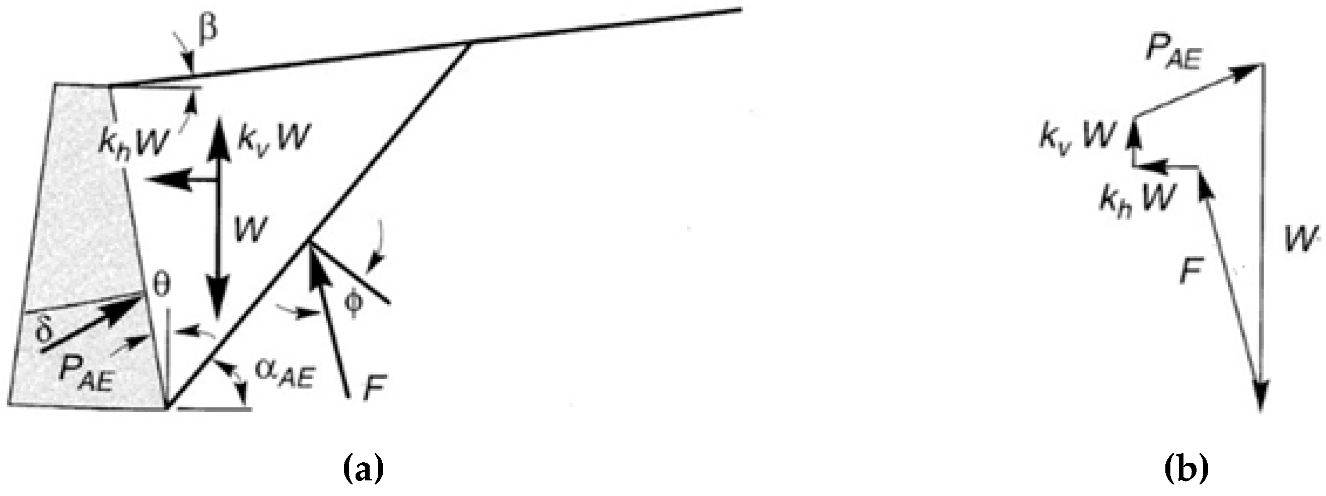
Figure 2.
Schematic diagram of Site 1.
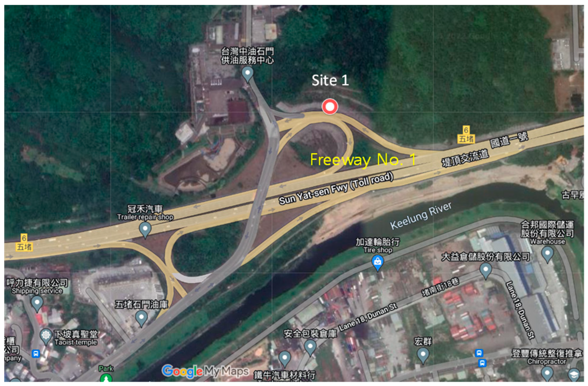
Figure 3.
Schematic diagram of Site 2 and Site 3.
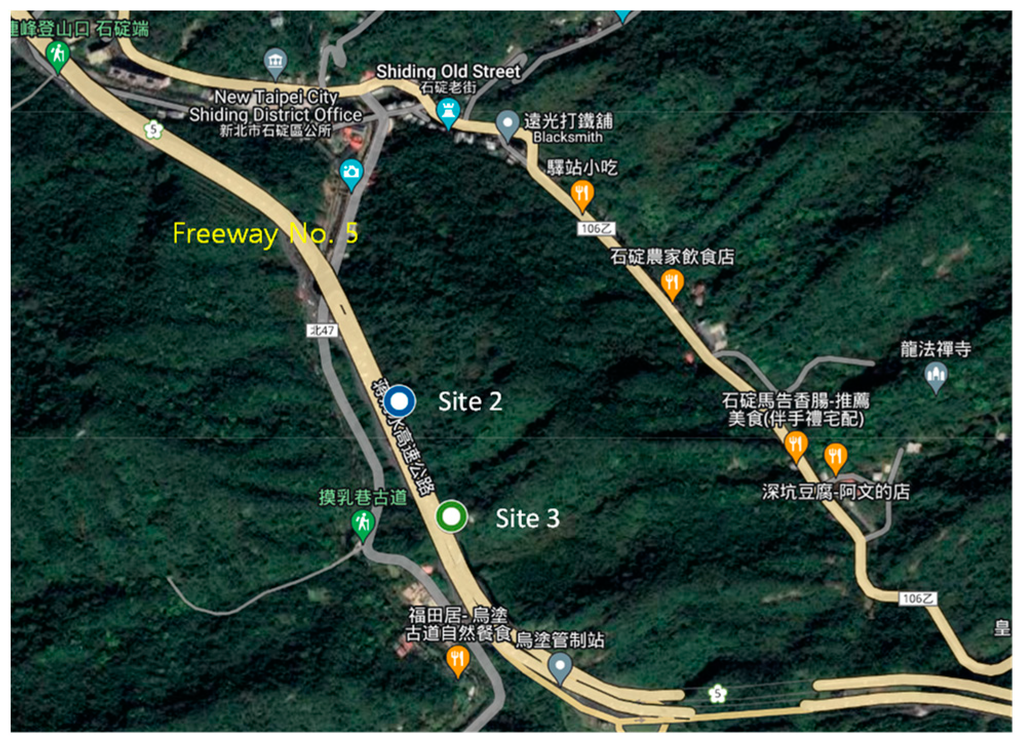
Figure 5.
Shading distribution diagram of total displacement with normal groundwater level at Site 1.
Figure 5.
Shading distribution diagram of total displacement with normal groundwater level at Site 1.
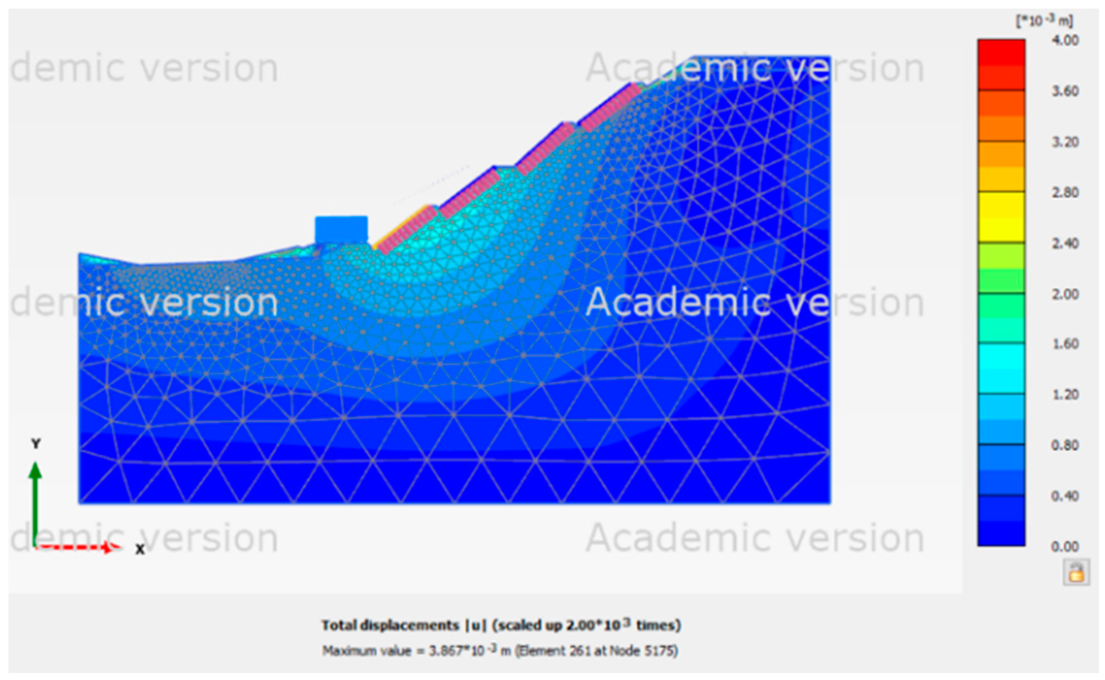
Figure 6.
Shading distribution diagram of total displacement with high groundwater level at Site 1.
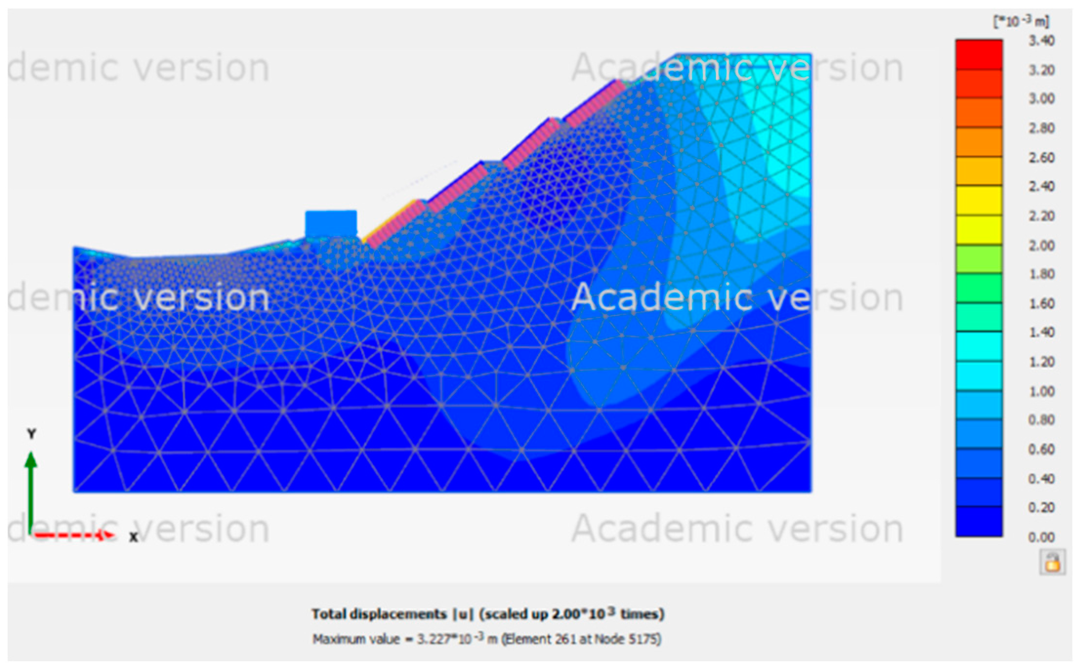
Figure 7.
Shading distribution diagram of total displacement with normal groundwater level and pseudo-static analysis for Site 1.
Figure 7.
Shading distribution diagram of total displacement with normal groundwater level and pseudo-static analysis for Site 1.
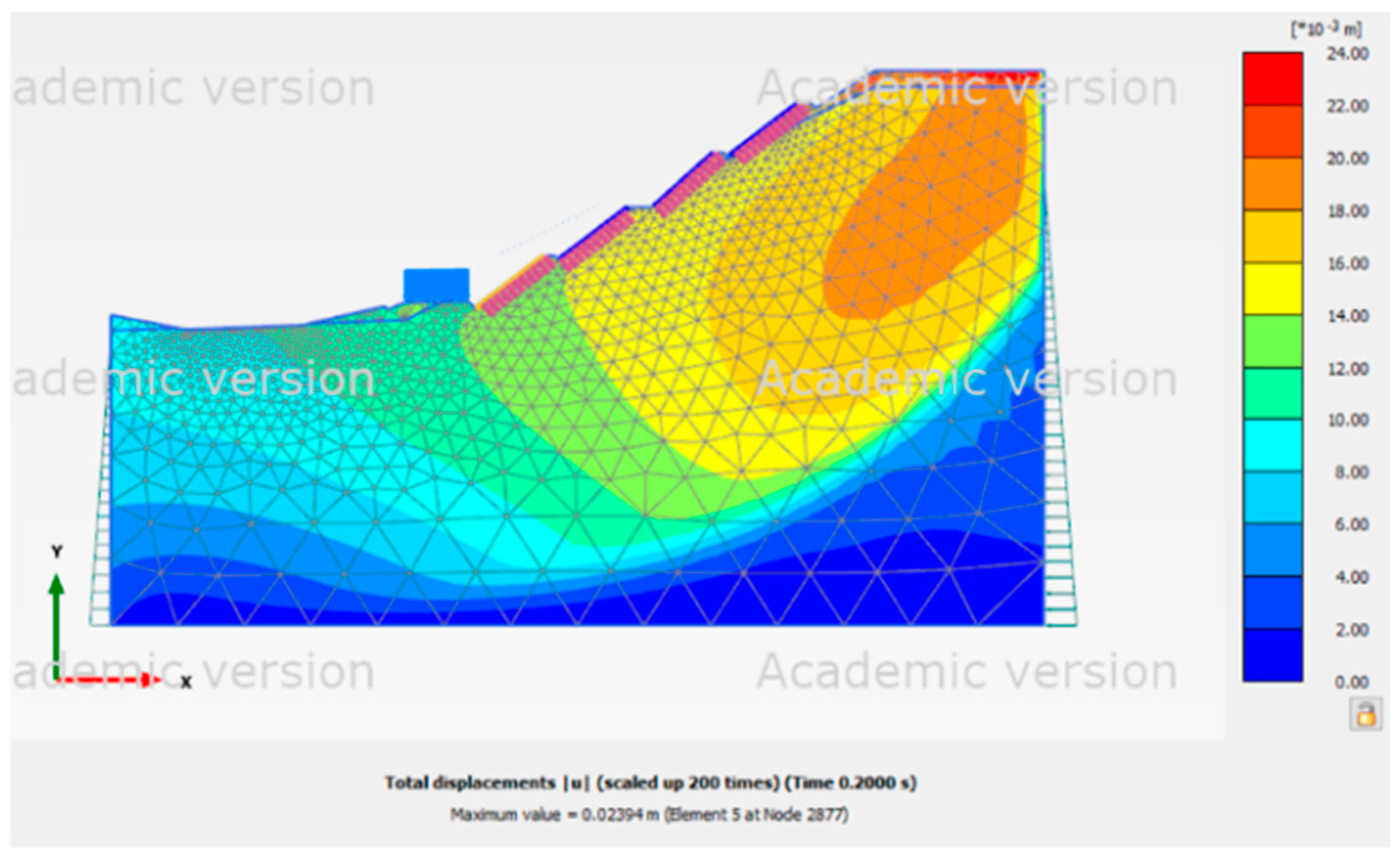
Figure 8.
PLAXIS 2D model for Site 2.
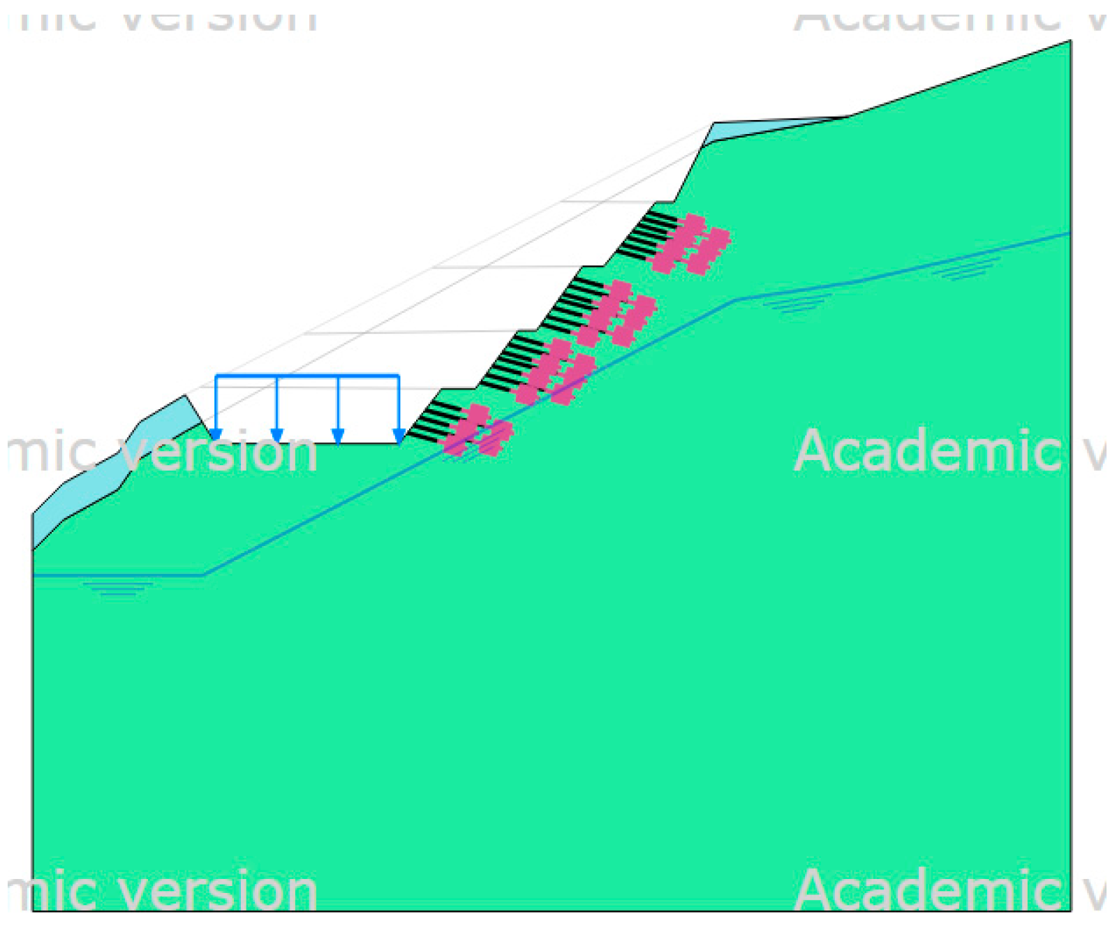
Figure 9.
Shading distribution diagram of total displacement with normal groundwater level for Site 2.
Figure 9.
Shading distribution diagram of total displacement with normal groundwater level for Site 2.
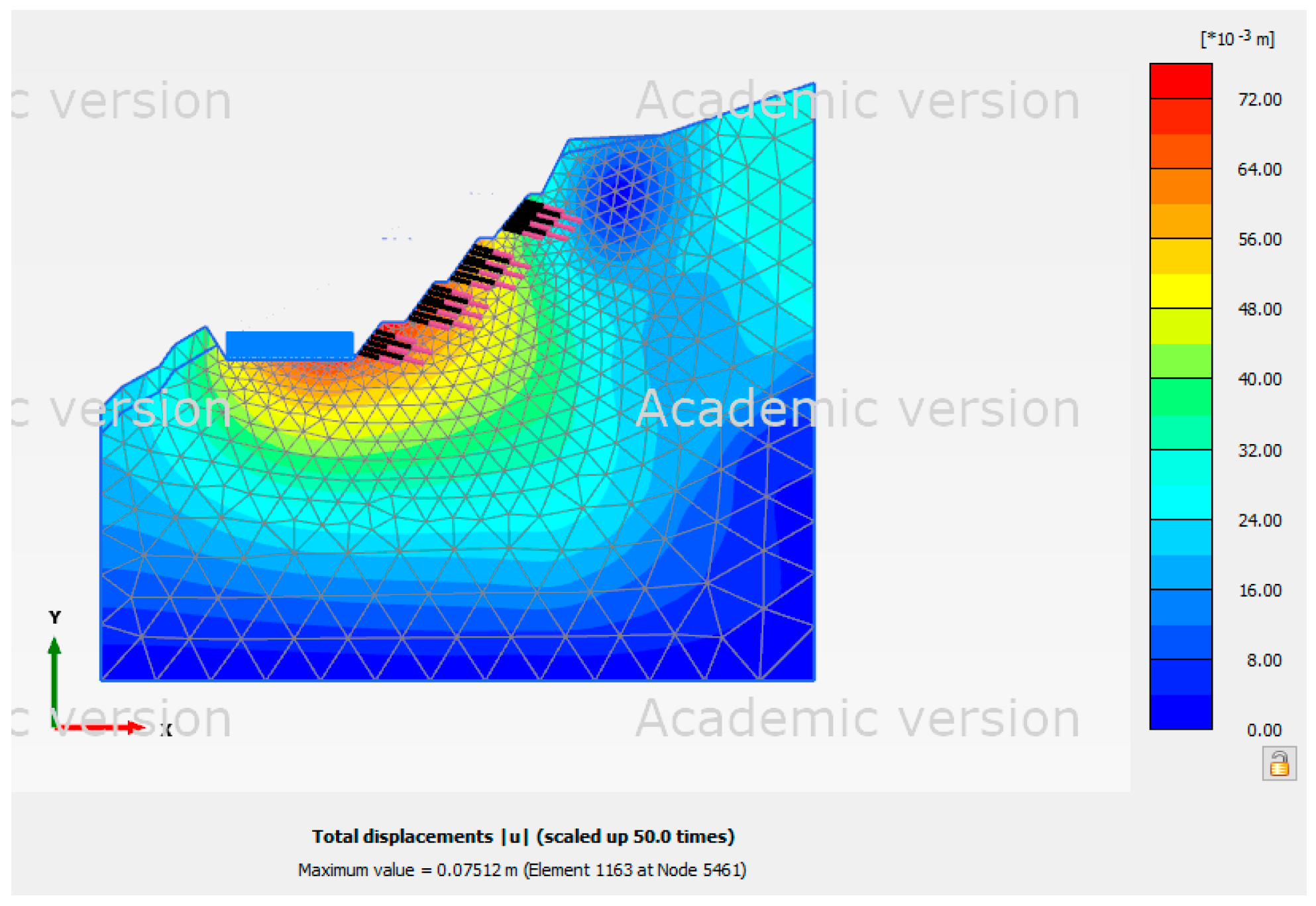
Figure 10.
Shading distribution diagram of total displacement with high groundwater level for Site 2.
Figure 10.
Shading distribution diagram of total displacement with high groundwater level for Site 2.
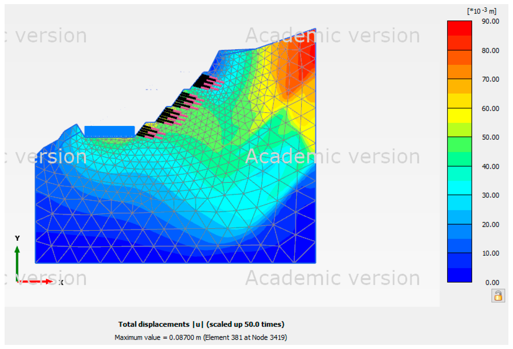
Figure 11.
Shading distribution diagram of total displacement with normal groundwater level and pseudo-static analysis for Site 2.
Figure 11.
Shading distribution diagram of total displacement with normal groundwater level and pseudo-static analysis for Site 2.
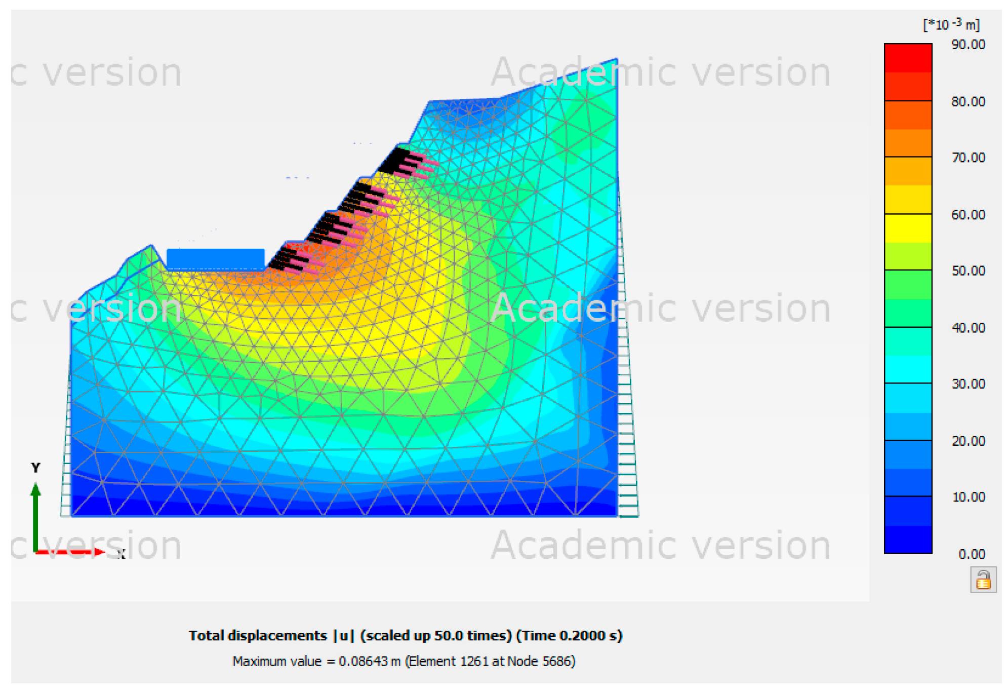
Figure 12.
PLAXIS 2D model for Site 3.
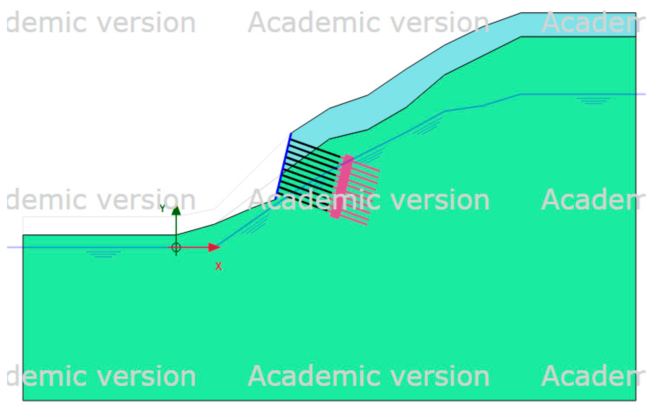
Figure 13.
Shading distribution diagram of total displacement with normal groundwater level for Site 3.
Figure 13.
Shading distribution diagram of total displacement with normal groundwater level for Site 3.
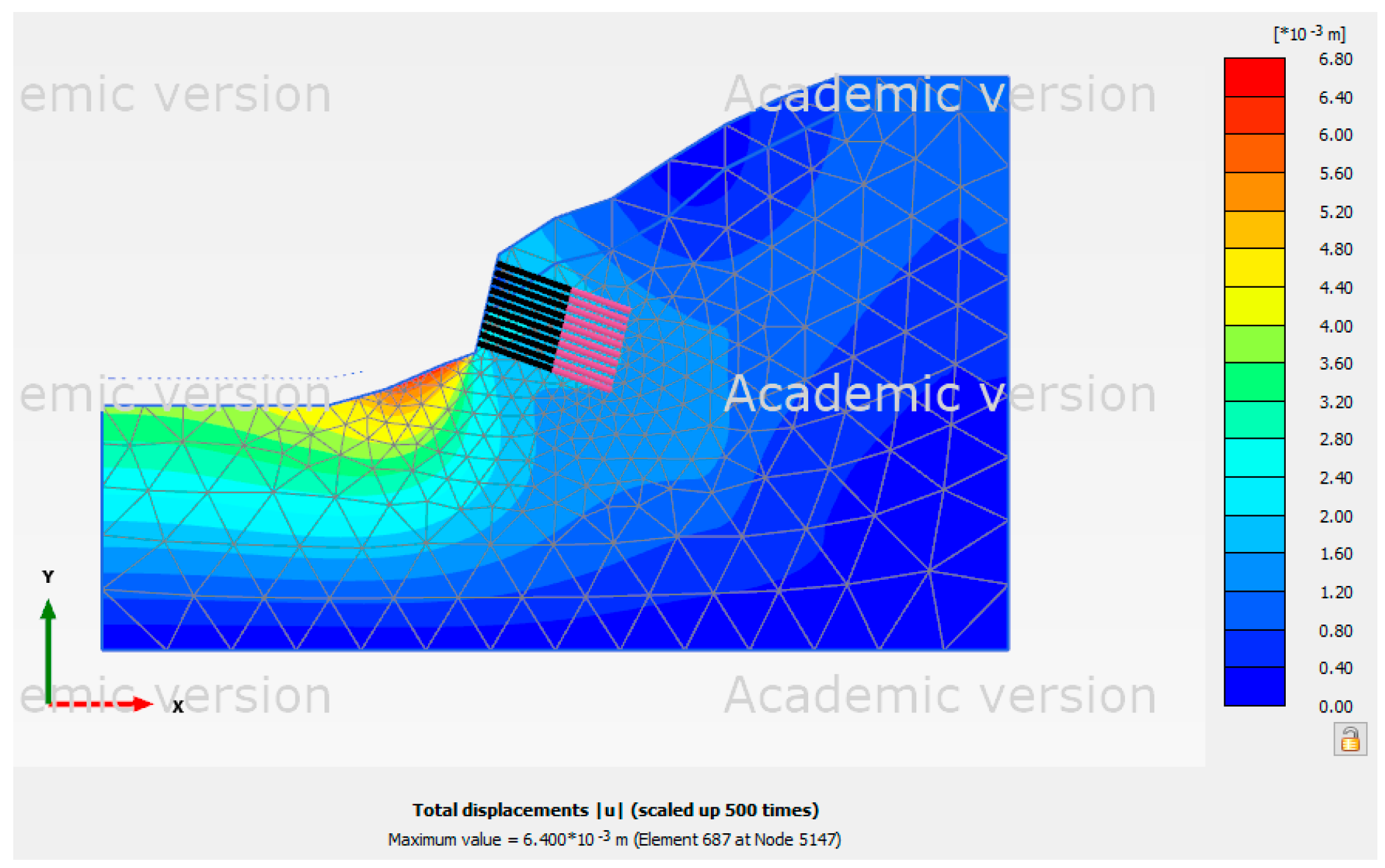
Figure 14.
Shading distribution diagram of total displacement with high groundwater level for Site 3.
Figure 14.
Shading distribution diagram of total displacement with high groundwater level for Site 3.
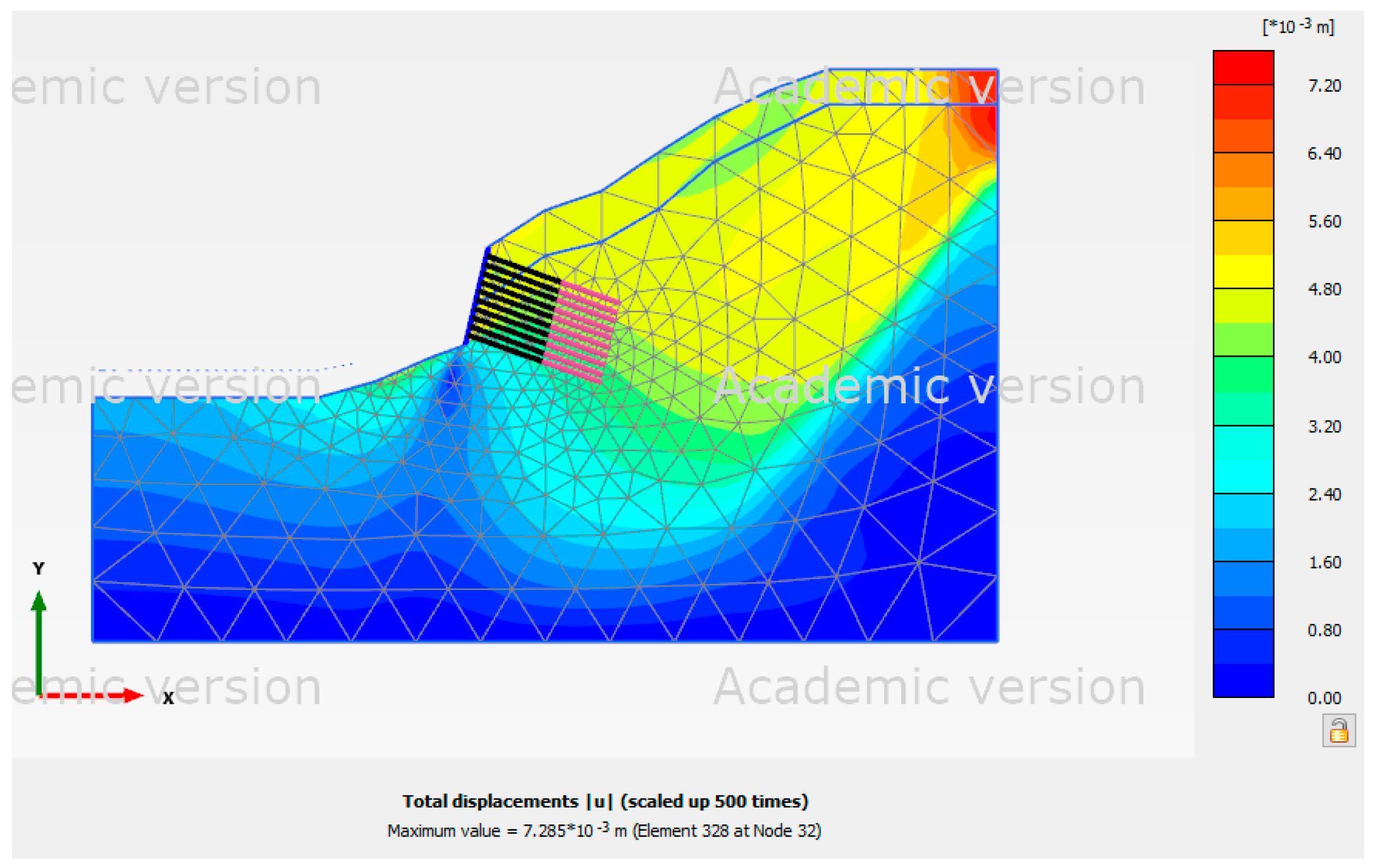
Figure 15.
Shading distribution diagram of total displacement with normal groundwater level and pseudo-static analysis for Site 3.
Figure 15.
Shading distribution diagram of total displacement with normal groundwater level and pseudo-static analysis for Site 3.
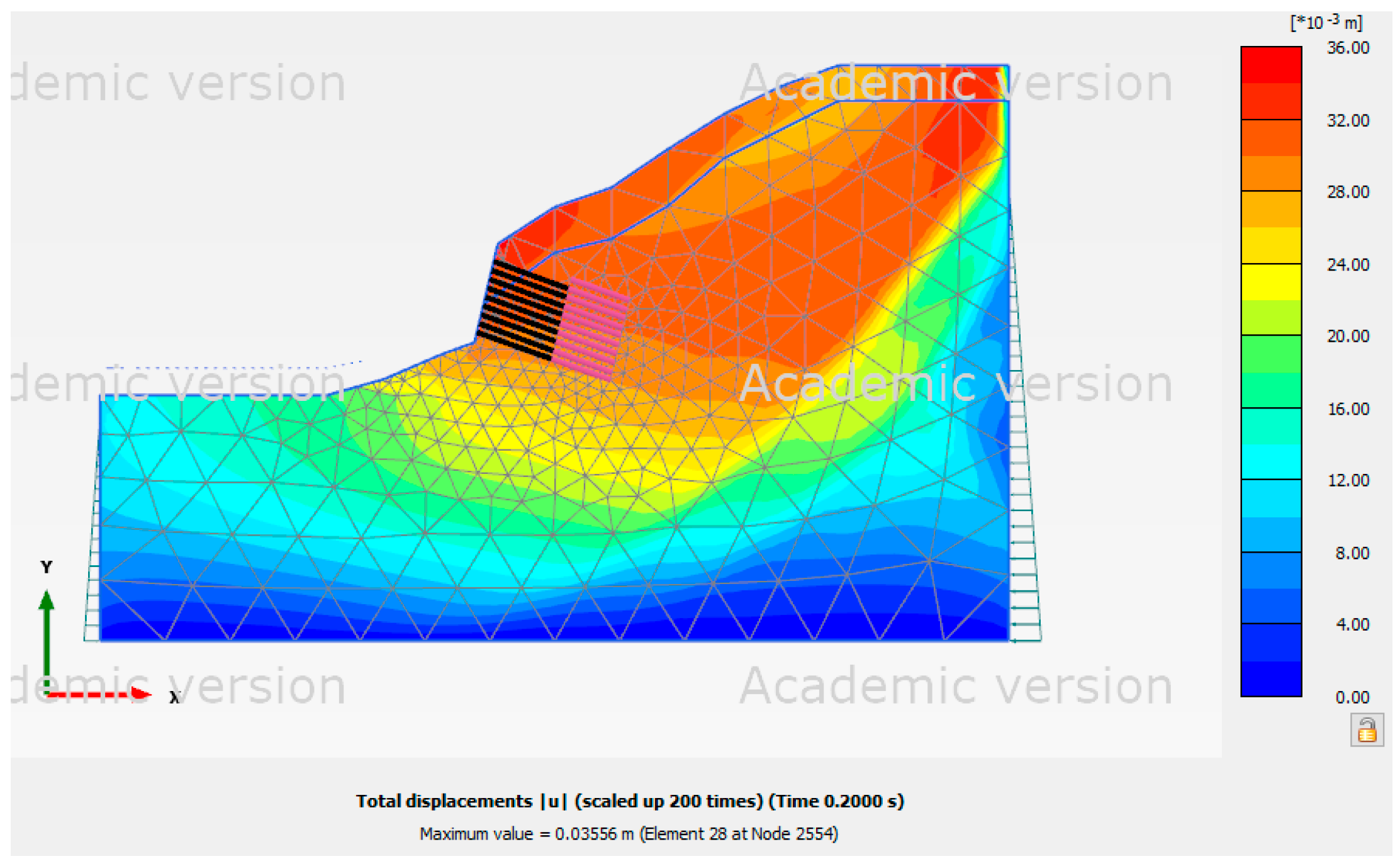
Table 4.
Displacement of Site 1 in various scenarios.
| scenarios |
∣u∣ (mm) |
(mm) | (mm) | ||
| max | min | max | min | ||
| Normal groundwater level | 3.87 | 1.62 | –0.30 | 3.56 | –0.50 |
| High groundwater level | 26.38 | 0.73 | –7.75 | 0 | –26.38 |
| Normal groundwater level and pseudo-static analysis | 23.94 | 0 | –20.44 | 2.47 | –13.30 |
Table 5.
Soil parameters of Site 2.
| Soil layer | Parameters | ||||||
|
(kN/m3) |
(kN/m3) |
E (kN/m2) |
ν |
c (kN/m2) |
φ ( ° ) |
ψ ( ° ) |
|
| Colluvium | 19.6 | 20.1 | 7×10⁴ | 0.3 | 10 | 28 | 0 |
| Weathered sandstone | 23.5 | 24.0 | 3×10⁵ | 0.3 | 50 | 30 | 0 |
Table 6.
Material parameters of anchor section of ground anchor of Site 2.
| Simulation elements | Young’s modulus (kN/m2) |
Unit weight (kN/m3) |
Diameter (cm) |
Horizontal spacing (m) |
Front end side friction resistance (kN/m) | Rear end side friction resistance (kN/m) |
|---|---|---|---|---|---|---|
| Embedded beam row element | 2.5 × 10⁷ | 10 | 20 | 3 | 95 | 95 |
Table 7.
Material parameters of free section of ground anchor of Site 2.
| Simulation elements | Material type | Axial stiffness (kN/m3) |
Horizontal spacing (m) |
Pre-force (kN/m) |
|---|---|---|---|---|
| Node-to-node anchor element | Elasticity | 7.53 × 10⁶ | 3 | 300 |
Table 8.
Displacement of Site 2 in various scenarios.
| scenario |
∣u∣ (mm) |
(mm) |
(mm) |
||
| max | min | max | min | ||
| Normal groundwater level | 75.12 | 17.84 | –29.35 | 73.27 | –30.22 |
| High groundwater level | 87.00 | 15.07 | –46.75 | 55.33 | –87.00 |
| Normal groundwater level and pseudo-static analysis | 86.43 | 0 | –56.94 | 73.92 | –40.24 |
Table 9.
Soil parameters of Site 3.
| Soil layer | Parameters | ||||||
|
(kN/m3) |
(kN/m3) |
E (kN/m2) |
ν |
c (kN/m2) |
φ ( ° ) |
ψ ( ° ) |
|
| Colluvial layer | 18.6 | 19.1 | 7 × 10⁴ | 0.3 | 10 | 28 | 0 |
| Interbedded sandstone and shale | 25.5 | 26.0 | 3 × 10⁵ | 0.3 | 50 | 35 | 5 |
Table 10.
Parameters of retaining wall materials of Site 3.
| Simulation elements | Material type | Axial stiffness (kN/m3) |
Flexural stiffness (kNm2/m) |
Weight (kN/m/m) |
ν |
|---|---|---|---|---|---|
| Plate element | Elasticity | 7.53 × 10⁶ | 7.2 | 0.17 |
Table 11.
Material parameters of anchor section of ground anchor of Site 3.
| Simulation elements | Young’s modulus (kN/m2) |
Unit weight (kN/m3) |
Diameter (cm) |
Horizontal spacing (m) |
Front end side friction resistance (kN/m) | Rear end side friction resistance (kN/m) |
|---|---|---|---|---|---|---|
| Embedded beam row element | 2.5 × 10⁷ | 10 | 20 | 3 | 43 | 43 |
Table 12.
Material parameters of free section of ground anchor of Site 3.
| Simulation elements | Material type | Axial stiffness (kN/m3) |
Horizontal spacing (m) |
Pre-force (kN/m) |
|---|---|---|---|---|
| Node-to-node anchor element | Elasticity | 2 × 10⁵ | 3.5 | 300 |
Table 13.
Displacement of Site 3 in various scenarios.
| scenario |
∣u∣ (mm) |
(mm) |
(mm) |
||
| max | min | max | min | ||
| Normal groundwater level | 6.40 | 1.62 | –2.38 | 6.31 | –1.31 |
| High groundwater level | 7.29 | 1.34 | –4.57 | 4.19 | –7.29 |
| Normal groundwater level and pseudo-static analysis | 35.56 | 0 | –34.95 | 9.15 | –25.62 |
Disclaimer/Publisher’s Note: The statements, opinions and data contained in all publications are solely those of the individual author(s) and contributor(s) and not of MDPI and/or the editor(s). MDPI and/or the editor(s) disclaim responsibility for any injury to people or property resulting from any ideas, methods, instructions or products referred to in the content. |
© 2024 by the authors. Licensee MDPI, Basel, Switzerland. This article is an open access article distributed under the terms and conditions of the Creative Commons Attribution (CC BY) license (http://creativecommons.org/licenses/by/4.0/).
Copyright: This open access article is published under a Creative Commons CC BY 4.0 license, which permit the free download, distribution, and reuse, provided that the author and preprint are cited in any reuse.


