
Submitted:
09 December 2024
Posted:
10 December 2024
You are already at the latest version
Abstract
The modelling of pan evaporation (Ep) trends in Slovak river basins was performed by utilizing artificial intelligence (AI) techniques algorithms to accurately forecast evaporation rates based on daily climate data spanning from 2010 to 2023 across eight sub-basins within the Slovak Republic. The findings derived from the AI modelling indicate that the river basins of Bodrog, Hornád, Ipeľ, Morava, Slaná, and Váh are experiencing increases in evaporation measurements, whereas the Dunaj and Hron rivers demonstrate declining trends. This divergence may suggest the presence of differing ecological factors that affect the evaporation dynamics associated with each river. In this study, a comprehensive set of 28 machine learning and deep learning models was employed, including: Machine Learning (ML): Linear Regression, Tree-Based, Support Vector Machines (both with and without Kernels), Ensemble, and Gaussian Process methods; Deep Learning (DL): Neural Networks (Narrow, Medium, Wide, Bilayered, and Trilayered). The Stepwise Linear Regression yielded the most optimal fit. The Minimum Redundancy Maximum Relevance (mRMR) method was utilized to assess the efficacy of feature selection by concentrating on both relevance and redundancy. The results suggest that placing greater emphasis on relative humidity (RH) and minimum temperature (tmin) may significantly enhance the predictive accuracy of the model.
Keywords:
1. Introduction
2. Materials and Methods
2.1. An Analytical Review of Climate Data
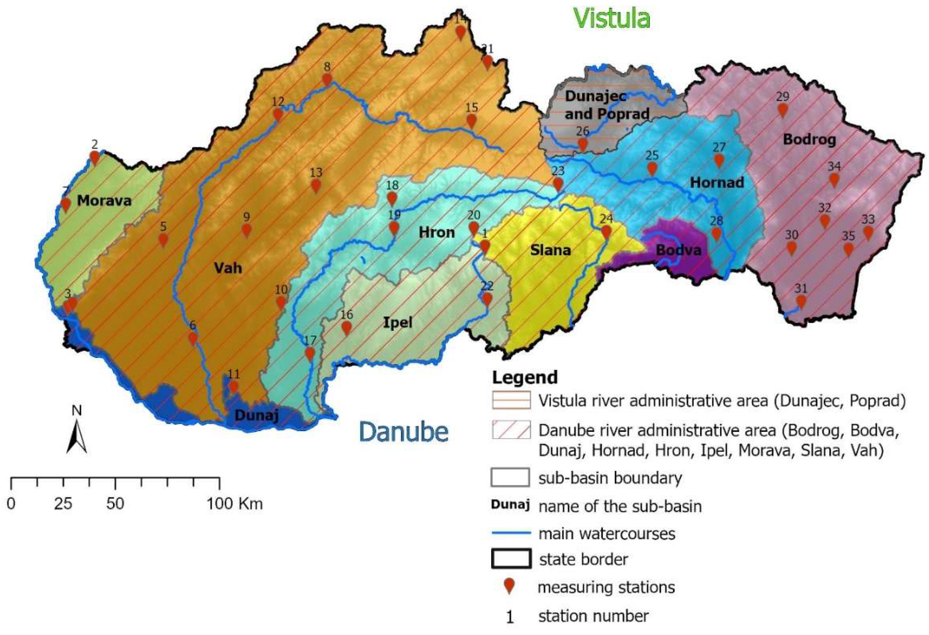
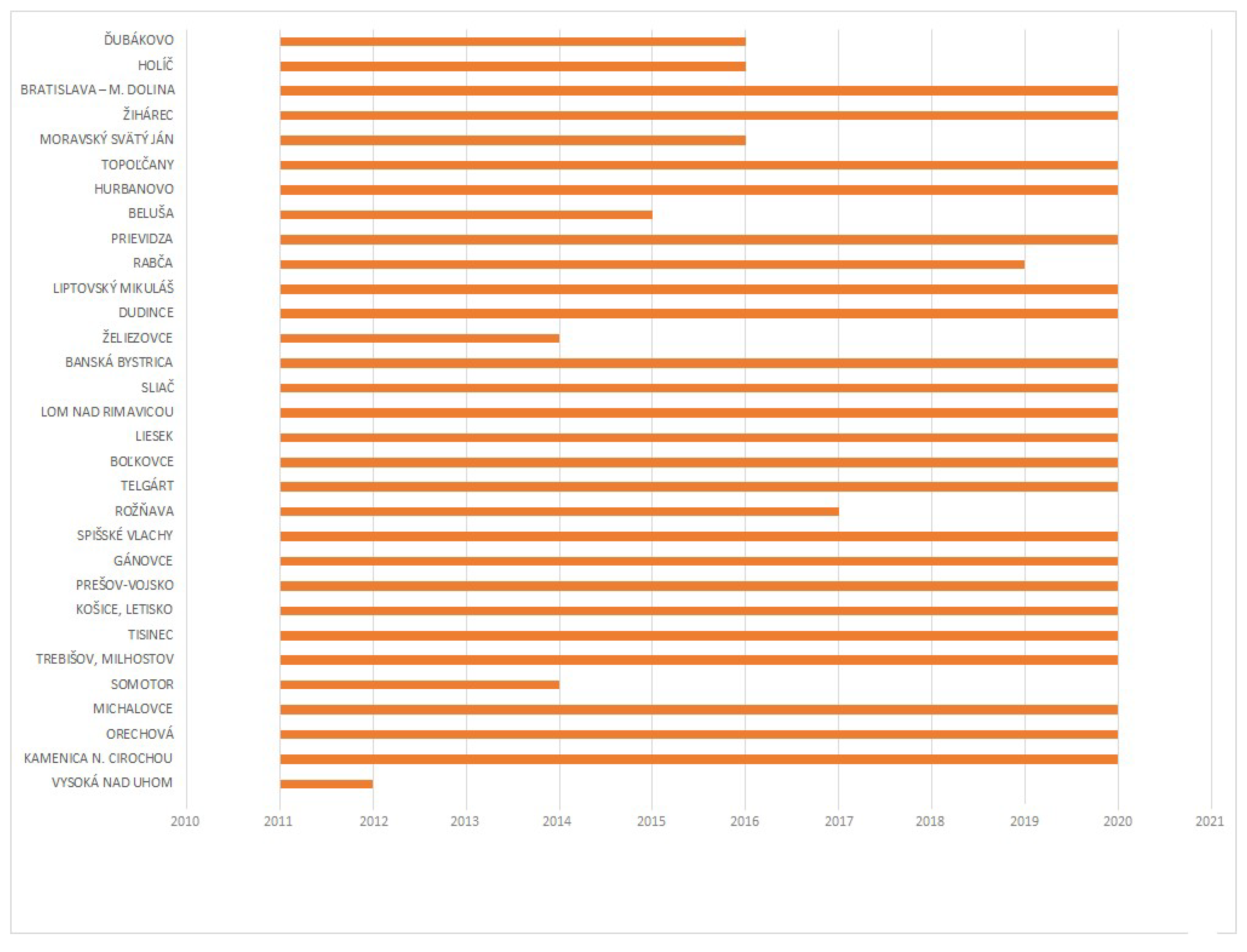
2.2. Data Description
2.3. Statistics and Machine Learning Toolbox Application
Linear Regression (LR) Methods
Tree-Based Methods
Support Vector Machines (SVM)
Efficient Linear (EL) Methods
Ensemble Methods (EM)
Gaussian Process Regression
Neural Networks (NN)
Kernels
3. Results
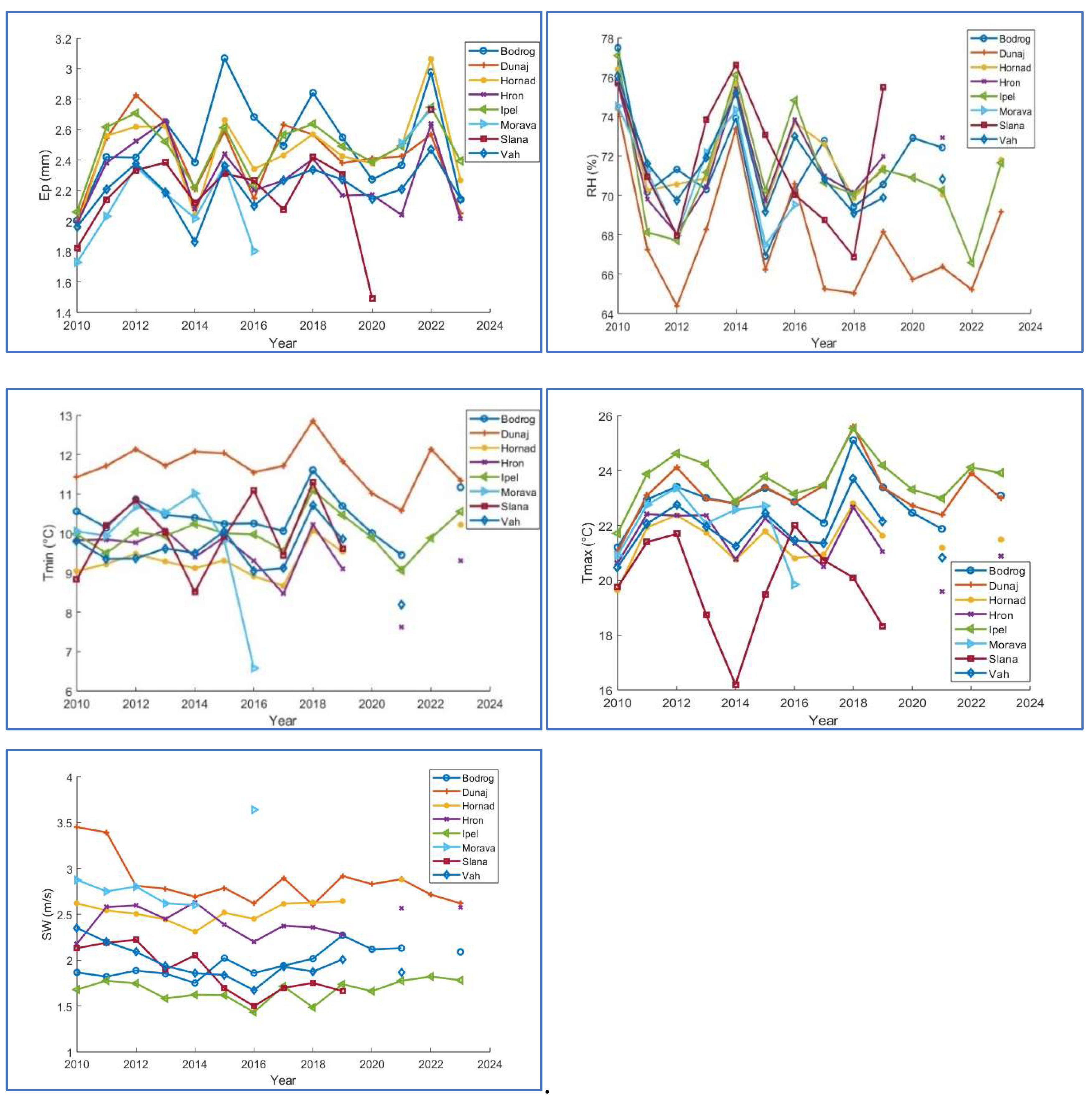
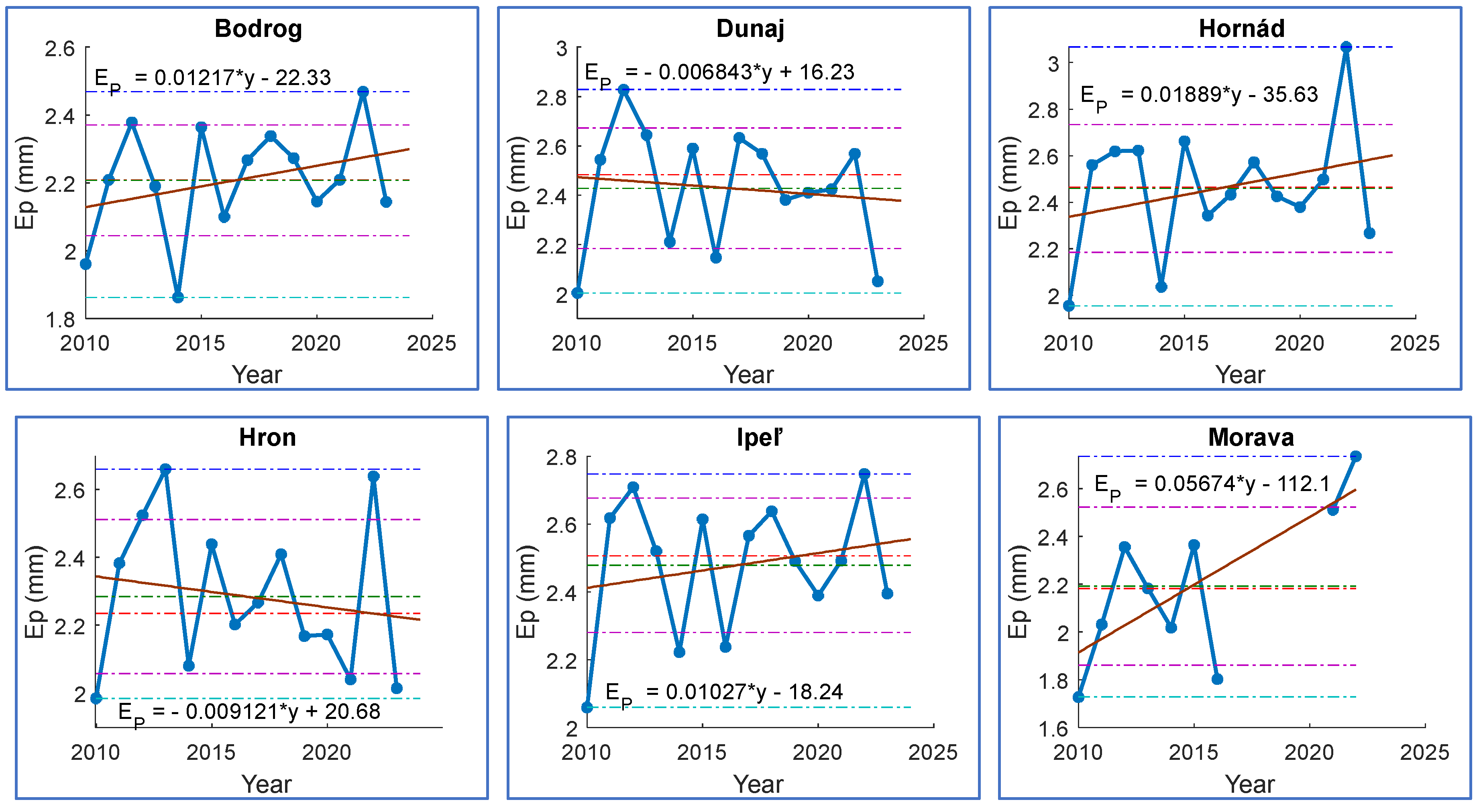
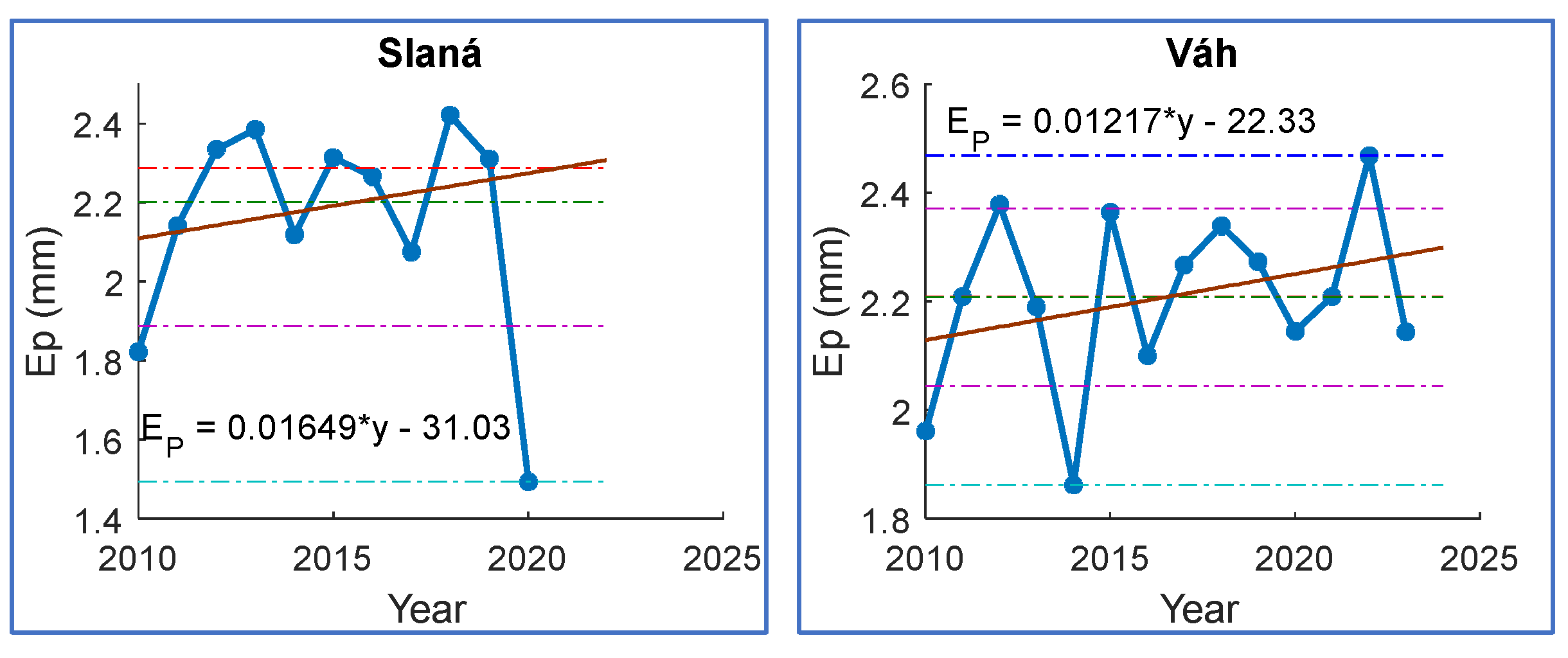
3.1. Changes in Ep Across River Basins
3.1.1. Ep Trend Analysis
- Bodrog river basin demonstrates a steady increase in measurements, with an annual change of +0,01057 mm, indicating a consistent rise in evaporation rates over time.
- Conversely, Dunaj river basin exhibits a slight decline, with an annual change of -0,006843 mm, suggesting a downward trend in evaporation.
- Hornád river basin shows a significant increase of +0,01889 mm per year.
- Similarly, Hron river basin reflects a decrease of -0,009121 mm annually.
- Ipeľ river basin records a modest increase of +0,01027 mm, indicating stable growth in its measurements, akin to that observed in Bodrog river basin.
- Morava river basin is notable for exhibiting the largest increase at +0,05674 mm per year.
- Slaná river basin also demonstrates a robust increase of +0,01649 mm.
- Finally, Váh river basin displays a consistent annual increase of +0,01217 mm, suggesting steady growth; however, this increase is less pronounced than those observed in other river basins.
3.2. AI Models’ Accuracy Evaluation
- ○
- The best model fit was evaluated for the LR models (1st and 2nd models) perform very well with RMSEs around 0.805 to 0.821 and R² values above 0.60, indicating that they can model dependence well.
- ○
- NN (Narrow, Medium, Wide, and Bilayered) have similar RMSE and MAE, while the results are also good, but not superior to traditional regression methods.
- ○
- SVM Models show relatively stable performances with RMSE between 0.882 - 0.900 and R² between 0.538 - 0.556, which are average results.
- ○
- Tree-based Models (Fine, Medium, Coarse) show worse performances, especially in predictions, with the highest RMSE value of 1.035 for Fine Trees.
- ○
- Gaussian Process Models get solid RMSE and MAE, with the best results around 0.877 RMSE. These models have the advantage of flexibility.
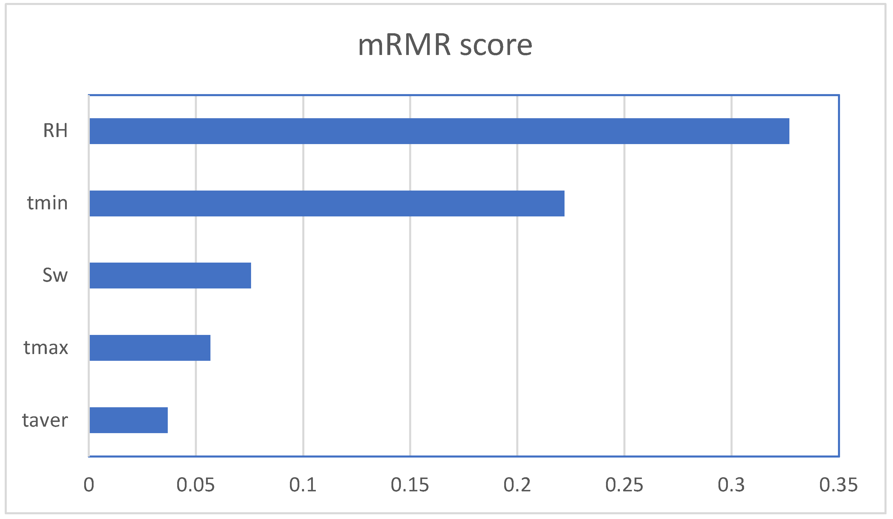
3.3. Climate Variables and Their Relation to the Ep
- Top Features: Relative humidity (RH) and minimum temperature (tmin) are the standout features, with RH being particularly critical to your analysis.
- Moderate Importance: Velocity (Sw) and maximum temperature (tmax) have moderate relevance but may not be as pivotal in influencing outcomes.
- Lowest Importance: Average temperature (taver) could be candidate for elimination or further consideration depending on the modelling approach, as it presents less relevance.
4. Discussion
5. Conclusions
Author Contributions
Funding
Institutional Review Board Statement
Informed Consent Statement
Data Availability Statement
Conflicts of Interest
References
- Šuhájková, P., Kožín, R., Beran, A., Melišová, E., Vizina, A., & Hanel, M. Update of empirical relationships for calculation of free water surface evaporation based on observation at Hlasivo station. Vodohospod. Tech.-Ekon. Inf. 2019, 61, 4-11. https://www.vtei.cz/en/2019/08/update-of-empirical-relationships-for-calculation-of-free-water-surface-evaporation-based-on-observation-at-hlasivo-station/ [In Czech].
- Kohut, M., Rožnovský, J., & Knozová, G. Měření výparu z vodní hladiny výparoměrem GGI-3000 v České republice Práce a studie 35. Praha: Český hydrometeorologický ústav, 2013, 95 s. ISBN 978-80-87577-16-5, ISSN 1210-7557. [In Czech].
- Fu, G., Charles, S.P. & Yu, J. A critical overview of pan evaporation trends over the last 50 years. Climatic Change 97, 193–214 (2009). [CrossRef]
- Jin, Y., Zhang, Y., Yang, X., Zhang, M., Guo, X.-B., Deng, Y., Hu, Y.-H., Lu, H.-Z., Tan, Z. H. Observed decreasing trend in pan evaporation in a tropical rainforest region during 1959–2021, Journal of Plant Ecology, Volume 17, Issue 1, February 2024, rtad033. [CrossRef]
- Abtew, W. Jayantha, O., & Nenad, I. Pan evaporation and potential evapotranspiration trends in South Florida . Hydrological Processes 2011, 25(6), 958-969. [CrossRef]
- Zhang, Q., Wang, W., Wang, S., Zhang, L. (2008). Increasing Trend of Pan Evaporation over the Semiarid Loess Plateau under a Warming Climate. J. Appl. Meteorol. Climatol. 2008, 55, 2007–2020. [CrossRef]
- Bai, H., Lu, X., Yang, X., Huang, J., Mu, X., Zhao, G., Gui, F., & Yue, C. Assessing impacts of climate change and human activities on the abnormal correlation between actual evaporation and atmospheric evaporation demands in southeastern China. Sustainable Cities and Society 2020, 56, 102075. [CrossRef]
- Golubev, V. S., Lawrimore, J. H., Groisman, Y. P., Speranskaya, N. A., Zhuravin, S. A., Menne, M. J., Peterson, T. C., & Malone, R. W. (2001). Evaporation changes over the contiguous United States and the former USSR: A reassessment, Geophysical Research Letters, No. 28, с. 2665. [CrossRef]
- Peterson, T., Golubev, V., & Groisman, P. Evaporation losing its strength. Nature 377. 1995., 687–688. [CrossRef]
- Stanhill, G., & Möller, M. Evaporative climate change in the British Isles, International Journal of Climatology 2007, No. 28, с. 1127. [CrossRef]
- Moonen, A. C., Ercoli, L., Mariotti , M., & Masoni, B. Climate change in Italy indicated by agrometeorological indices over 122 years, Agricultural and Forest Meteorology 2002, No. 111, с. 13. [CrossRef]
- Liu, B., Xu, M., Henderson, M., & Gong, W. A spatial analysis of pan evaporation trend in China, 1955-2000, Journal of Geophysical Research Atmospheres 2004, No. 109. [CrossRef]
- Shen, Y., Liu, C., Liu, M., Zeng, Y., & Tian, C. Change in pan evaporation over the past 50 years in the arid region of China, Hydrological Processes 2009, No. 24, с. 225. [CrossRef]
- Xu, Y.-P., Pan, S., Gao, C., Fu, G., & Chiang, Y.-M. Historical pan evaporation changes in the Qiantang River Basin, East China, International Journal of Climatology 2015, No. 36, с. 1928. [CrossRef]
- Yang, H., & Yang, D. Climatic factors influencing changing pan evaporation across China from 1961 to 2001, Journal of Hydrology 2012, No. 414-415, с. 184. [CrossRef]
- Chen, D., Gao, G., Xu, C.-Y., Guo, J., & Ren, G. Comparison of the Thornthwaite method and pan data with the standard Penman-Monteith estimates of reference evapotranspiration in China, Climate Research 2005, No. 28, с. 123. [CrossRef]
- Thomas, A. Spatial and temporal characteristics of potential evapotranspiration trends over China, International Journal of Climatology 2000, No. 20, с. 381. [CrossRef]
- Wang, K., & Dickinson, R. E. A review of global terrestrial evapotranspiration: Observation, modeling, climatology, and climatic variability, Reviews of Geophysics 2012, No. 50. [CrossRef]
- Zhang, L., Seydou, T., Yuanla, C., Yufeng, L., Ge, Z., Bo, L., Guy, F., Karthikeyan, R., & Vijay, S. Assessment of spatiotemporal variability of reference evapotranspiration and controlling climate factors over decades in China using geospatial techniques, Agricultural Water Management 2019, No. 213, с. 499 Management 2019, No. 213, с. 499. [CrossRef]
- Croitoru, A.-E., Piticar, A., Dragotă, C. S., & Burada, D. C. Recent changes in reference evapotranspiration in Romania, Global and Planetary Change 2013, No. 111, с. 127. [CrossRef]
- Chattopadhyay, N., & Hulme, M. Evaporation and potential evapotranspiration in India under conditions of recent and future climate change, Agricultural and Forest Meteorology 1997, No. 87, с. 55. [CrossRef]
- Hobbins, M. T., Dai, A., Roderick, M. L., & Farquhar, G. D. Revisiting the parameterization of potential evaporation as a driver of long-term water balance trends, Geophysical Research Letters 2008, No. 35. [CrossRef]
- Abtew, W., Obeysekera, J., & Iricanin, N. Pan evaporation and potential evapotranspiration trends in South Florida, Hydrological Processes 2010, No. 25, с. 958. [CrossRef]
- Hember, R. A., Coops, N. C., & Spittlehouse, D. L. Spatial and Temporal Variability of Potential Evaporation across North American Forests. Hydrology 2017, 4(1), 5. [CrossRef]
- Damborská, I., & Lapin, M. Changes and variability of evapotranspiration sums in Slovakia in 1951–2021. Contributions to Geophysics and Geodesy 2023, 53(3), 241-270. [CrossRef]
- Hrvoľ, J., Horecká, V., Škvarenina, J., Střelcová, K., & Škvareninová, J. Long-term results of evaporation rate in xerothermic Oak altitudinal vegetation stage in Southern Slovakia. Biologia 64. 2009, 605–609. [CrossRef]
- Novák, V., Danko, M., Holko., L. (2018). Hydrological research in the conditions of ongoing climate change. Bratislava: Veda, 2018, s. 51-93. ISBN 978-80-224-1691-7 978-80-224-1691-7.
- Eyring, V., Collins, W. D., Gentine, P., et al. Pushing the frontiers in climate modelling and analysis with machine learning. Nat. Clim. Chang. 14. 2024, 916–928. [CrossRef]
- Novotná, B., Jurík, Ľ., Čimo, J., Palkovič, J., Chvíla, B., Kišš, V. Machine Learning for Pan Evaporation Modeling in Different Agroclimatic Zones of the Slovak Republic (Macro-Regions). Sustainability 2022, 14, 3475. [CrossRef]
- Ren., C., Ren, G., Zhang, P., Kealdrup, S., & Qin, T. Y. Urbanization Significantly Affects Pan-Evaporation Trends in Large River Basins of China Mainland. Land 2021, 10(4):407.
- Abed, M., Imteaz, M. A., Ahmed, A. N. et al. Modelling monthly pan evaporation utilising Random Forest and deep learning algorithms. Sci Rep 12. 2022, 13132. [CrossRef]
- Amoo, T. O. Integrated hydrological modelling for sustainable water allocation planning: Mkomazi Basin, South Africa case study. 2018. [CrossRef]
- Benjamin, S. G., Brown, J. M., Brunet, G., Lynch, P., Saito, K., & Schlatter, T. W. 100 Years of Progress in Forecasting and NWP Applications. Meteorological Monographs, 59. 2019, 13.1-13.67. [CrossRef]
- Mao, Y., Li, Y., Teng, F., Sabonchi, A. K. S., Azarafza, M., & Zhang, M. Utilizing Hybrid Machine Learning and Soft Computing Techniques for Landslide Susceptibility Mapping in a Drainage Basin. Water 2024, 16(3), 380. [CrossRef]
- Drogkoula, M., Kokkinos, K., & Samaras, N. A. Comprehensive Survey of Machine Learning Methodologies with Emphasis in Water Resources Management. Appl. Sci. 2023, 13, 12147. [CrossRef]
- Ministry of Environment of the Slovak Republic Water Plan of the Slovak Republic – Update 2021. Summary Information. Porter, s.r.o. 2023. ISBN 978-80-8213-122-5. https://download.sazp.sk/2023/WPS-2021-Summary-Information-web.pdf.
- SHMÚ. Climate atlas of Slovakia. Slovenský hydrometeorologický ústav. Bratislava. 2015.
- Climatic Conditions of the Slovak Republic (Klimatické Pomery Slovenskej Republiky) 2022. https://www.shmu.sk/sk/?page=1064 (In Slovak).
- Slovak Environmental Agency. Atlas of the Slovak Republic - Web map application, 2024. https://app.sazp.sk/atlassr/.
- MathWorks. Statistics and Machine Learning Toolbox Analyze and model data using statistics and machine learning, 2024. https://www.mathworks.com/products/statistics.html.
- Zhao, Z., Anand, R., & Wang, M. Maximum Relevance and Minimum Redundancy Feature Selection Methods for a Marketing Machine Learning Platform. 2019 IEEE International Conference on Data Science and Advanced Analytics (DSAA), 442-452.
- Alsumaiei, A. A. Utility of Artificial Neural Networks in Modeling Pan Evaporation in Hyper-Arid Climates. Water 2020, 12, 1508. [CrossRef]
- Brutsaert, W., & Parlange, M. Hydrologic Cycle Explains the Evaporation Paradox. Nature 396. 1998, 30. [CrossRef]
- Elbeltagi, A., Heddam, S., Katipoğlu, O., Alsumaiei, A., & Al-Mukhtar, M. Advanced long-term actual evapotranspiration estimation in humid climates for 1958–2021 based on machine learning models enhanced by the RReliefF algorithm. Journal of Hydrology Regional Studies 2024. [CrossRef]
- Elbeltagi, A., Al-Mukhtar, M., Kushwaha, N.L., Nadhir, A.-A., & Vishwakarmaet, D. K. Forecasting monthly pan evaporation using hybrid additive regression and data-driven models in a semi-arid environment. Appl Water Sci 13, 42. 2023. [CrossRef]
- Massari, C., Avanzi, F., Bruno, G., Gabellani, S., Penna, D., & Camici, S. Evaporation enhancement drives the European water-budget deficit during multi-year droughts, Hydrol. Earth Syst. Sci., 26. 2022, 1527–1543. [CrossRef]
- Helm, J. M., Swiergosz, A. M., Haeberle, H. S., Karnuta, J. M., Schaffer, J. L., Krebs, V. E., Spitzer, A. I., & Ramkumar, P. N. Machine Learning and Artificial Intelligence: Definitions, Applications, and Future Directions. Curr Rev Musculoskelet Med. 2020 Feb; 13(1):69-76. /: https. [CrossRef]
- Miller, J. A., Aldosari, M., Saeed, F., Barna, N. H., Rana, S., Arpinar, I. B., & Liu, N., A Survey of Deep Learning and Foundation Models for Time Series Forecasting. 1, 1. 2024, 35 pages. [CrossRef]
- Solís, M., & Calvo-Valverde, L.-A. Explaining When Deep Learning Models Are Better for Time Series Forecasting. Engineering Proceedings 2024, 68(1), 1. [CrossRef]
- Westergaard, G., Erden, U., Mateo, O. A., Lampo, S. M., Akinci, T. C., & Topsakal, O. Time Series Forecasting Utilizing Automated Machine Learning (AutoML): A Comparative Analysis Study on Diverse Datasets. Information 2024, 15(1), 39 Datasets. [CrossRef]
- Kisi, O., Mirboluki, A., Naganna, S. R., Malik, A., Kuriqi, A., & Mehraein, M. Comparative evaluation of deep learning and machine learning in modelling pan evaporation using limited inputs, Hydrological Sciences Journal 2022. [CrossRef]
- Roderick, M. L., & Farquhar, G. D. Changes in Australian pan evaporation from 1970 to 2002, International Journal of Climatology 2004, No. 24, с. 1077. [CrossRef]
- Roderick, M. L., & Farquhar, G. D. Changes in New Zealand pan evaporation since the 1970s, International Journal of Climatology 2005, No. 25, с. 2031. [CrossRef]

| No. | Station Name | River Basin | District |
|---|---|---|---|
| 1 | Ďubákovo | Slaná | Banskobystrický |
| 2 | Holíč | Morava | Trnavský |
| 3 | Bratislava, Mlynská Dolina | Dunaj | Bratislavský |
| 4 | Bratislava-Koliba | Dunaj | Bratislavský |
| 5 | Jaslovské Bohunice | Váh | Trnavský |
| 6 | Žihárec | Váh | Nitriansky |
| 7 | Moravský Svätý Ján | Morava | Trnavský |
| 8 | Dolný Hričov | Váh | Žilinský |
| 9 | Topoľčany | Váh | Nitriansky |
| 10 | Mochovce | Váh | Nitriansky |
| 11 | Hurbanovo | Dunaj | Nitriansky |
| 12 | Beluša | Váh | Trenčiansky |
| 13 | Prievidza | Váh | Trenčiansky |
| 14 | Rabča | Váh | Žilinský |
| 15 | Liptovský Mikuláš, Ondrášová | Váh | Žilinský |
| 16 | Dudince | Ipeľ | Banskobystrický |
| 17 | Želiezovce | Hron | Nitriansky |
| 18 | Banská Bystrica, Zelená | Hron | Banskobystrický |
| 19 | Sliač | Hron | Banskobystrický |
| 20 | Lom nad Rimavicou | Slaná | Banskobystrický |
| 21 | Liesek | Váh | Žilinský |
| 22 | Boľkovce | Ipeľ | Banskobystrický |
| 23 | Telgárt | Hron | Banskobystrický |
| 24 | Rožňava | Slaná | Košický |
| 25 | Spišské Vlachy | Hornád | Košický |
| 26 | Gánovce | Hornád | Prešovský |
| 27 | Prešov – Army | Hornád | Prešovský |
| 28 | Košice, Airport | Hornád | Košický |
| 29 | Tisinec | Bodrog | Prešovský |
| 30 | Trebišov, Milhostov | Bodrog | Košický |
| 31 | Somotor | Bodrog | Košický |
| 32 | Michalovce | Bodrog | Košický |
| 33 | Orechová | Bodrog | Košický |
| 34 | Kamenica nad Cirochou | Bodrog | Prešovský |
| 35 | Vysoká Nad Uhom | Bodrog | Košický |
| No. | Code | Station Name | Climate data | ||
|---|---|---|---|---|---|
| Starting date | Ending date | ||||
| 1 | 665 | Ďubákovo | 1.1.2007 | 6/30/2016 | |
| 2 | 11,8 | Holíč | 1.1.2007 | 6/30/2016 | |
| 3 | 11,81 | Bratislava – M. Dolina | 39083 | 12/31/2023 | |
| 4 | 11,813 | Bratislava-Koliba | 1.1.2007 | 12/31/2019 | |
| 5 | 11,819 | Jaslovské Bohunice | 1.1.2007 | 12/31/2019 | |
| 6 | 11,82 | Žihárec | 1.1.2007 | 12/31/2023 | |
| 7 | 11,835 | Moravský Svätý Ján | 1.1.2007 | 12/31/2019 | |
| 8 | 11,841 | Dolný Hričov | 1.1.2007 | 12/31/2023 | |
| 9 | 11847 | Topoľčany | 1.1.2007 | 12/31/2023 | |
| 10 | 11,856 | Mochovce | 1.1.2007 | 12/31/2019 | |
| 11 | 11,858 | Hurbanovo | 1.1.2007 | 12/31/2023 | |
| 12 | 11,862 | Beluša | 1.1.2007 | 12/31/2019 | |
| 13 | 11,867 | Prievidza | 1.1.2007 | 12/31/2023 | |
| 14 | 11,869 | Rabča | 1.1.2007 | 12/31/2019 | |
| 15 | 11,878 | Liptovský Mikuláš | 1.1.2007 | 12/31/2023 | |
| 16 | 11880 | Dudince | 1.1.2007 | 12/31/2023 | |
| 17 | 11,881 | Želiezovce | 1.1.2007 | 12/31/2014 | |
| 18 | 11,898 | Banská Bystrica | 1.1.2007 | 12/31/2019 | |
| 19 | 11903 | Sliač | 1.1.2007 | 12/31/2023 | |
| 20 | 11,91 | Lom nad Rimavicou | 1.1.2007 | 12/31/2019 | |
| 21 | 11,918 | Liesek | 1.1.2007 | 12/31/2023 | |
| 22 | 11927 | Boľkovce | 1.1.2007 | 12/31/2023 | |
| 23 | 11,938 | Telgárt | 1.1.2007 | 12/31/2023 | |
| 24 | 11,944 | Rožňava | 1.1.2007 | 10/30/2017 | |
| 25 | 11,949 | Spišské Vlachy | 1.1.2007 | 12/31/2019 | |
| 26 | 11,952 | Gánovce | 1.1.2007 | 12/31/2023 | |
| 27 | 11955 | Prešov-vojsko | 1.1.2007 | 12/31/2023 | |
| 28 | 11968 | Košice, letisko | 1.1.2007 | 12/31/2023 | |
| 29 | 11976 | Tisinec | 1.1.2007 | 12/31/2023 | |
| 30 | 11978 | Trebišov, Milhostov | 1.1.2007 | 12/31/2023 | |
| 31 | 11,979 | Somotor | 1.1.2007 | 11/30/2015 | |
| 32 | 11982 | Michalovce | 1.1.2007 | 12/31/2023 | |
| 33 | 11984 | Orechová | 1.1.2007 | 12/31/2023 | |
| 34 | 11,993 | Kamenica N. Cirochou | 1.1.2007 | 12/31/2023 | |
| 35 | 11,995 | Vysoká nad Uhom | 1.1.2007 | 12/31/2019 | |
| 36 | 11855 | Nitra - Veľké Janíkovce | 1.1.2020 | 12/31/2023 | |
| Legend | |||||
| complete data | |||||
| some records are missing | |||||
| higher located stations - the measurement started later, e.g. in May | |||||
| the station has stopped measuring or the data is incomplete | |||||
| the station has been translated several times | |||||
| measurements finished | |||||
| River Basin | Number of Observations |
Mean | Median | Standard Deviation | Coefficient of Variation | Range | Quartiles | Whiskers |
|---|---|---|---|---|---|---|---|---|
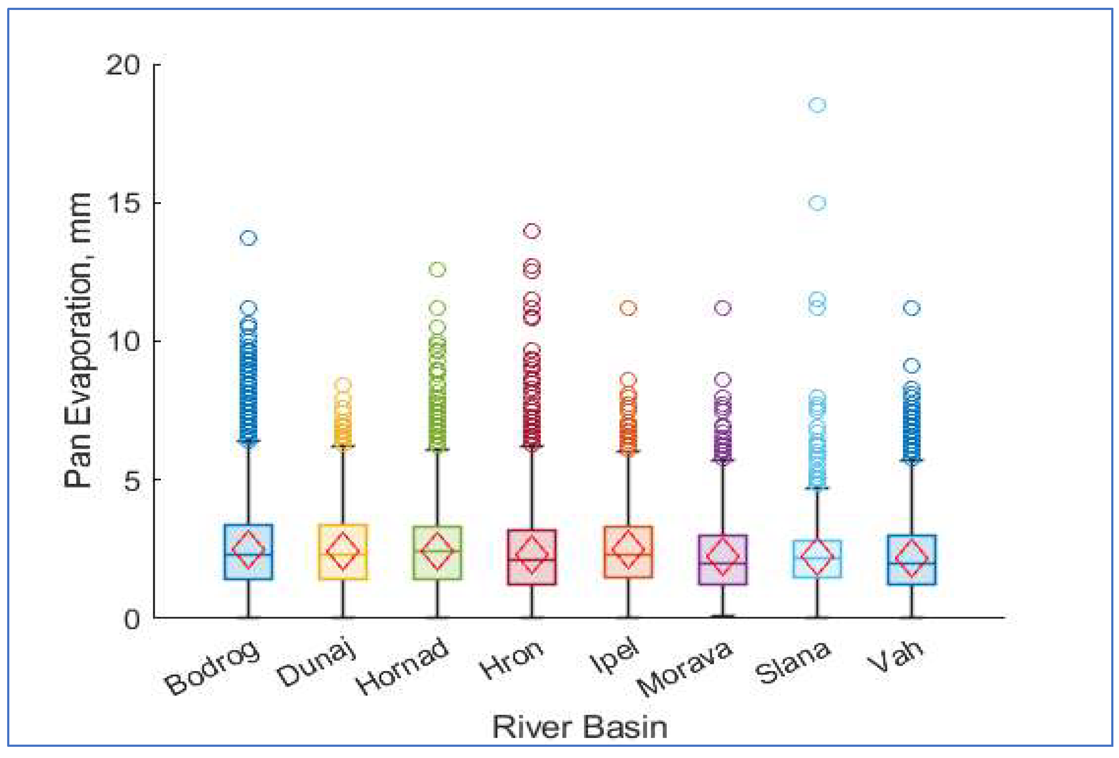
| Bodrog | 16 444 | 2.51 | 2.23 | 1.5 | 0.6 | 13.7 | [1.4 3.4] | [0 6.4] |
| Dunaj | 5 880 | 2.42 | 2.3 | 1.36 | 0.56 | 8.4 | [1.4 3.35] | [0 6.2] |
| Hornád | 11 047 | 2.46 | 2.4 | 1.41 | 0.57 | 12.6 | [1.4 3.3] | [0 6.1] |
| Hron | 8 827 | 2.3 | 2.1 | 1.42 | 0.62 | 14 | [1.2 3.2] | [0 6.2] |
| Ipeľ | 5 901 | 2.48 | 2.3 | 1.29 | 0.52 | 11.2 | [1.5 3.3] | [0 6] |
| Morava | 3 148 | 2.21 | 2 | 1.37 | 0.62 | 11.1 | [1.2 3] | [0.1 5.7] |
| Slaná | 3 252 | 2.21 | 2.2 | 1.16 | 0.52 | 18.5 | [1.5 2.8] | [0 4.7] |
| Váh | 21 237 | 2.2 | 2 | 1.32 | 0.6 | 11.2 | [1.2 3] | [0 5.7] |
| River Basin Comparison | Difference between Means | Lower Limit | Higher Limit |
|---|---|---|---|
| Bodrog vs Dunaj | 0.0831 | 0.0166 | 0.1497 |
| Bodrog vs Hornád | 0.0481 | -0.0076 | 0.1038 |
| Bodrog vs Hron | 0.2110 | 0.1511 | 0.2709 |
| Bodrog vs Ipeľ | 0.0301 | -0.0339 | 0.0942 |
| Bodrog vs Morava | 0.2995 | 0.2148 | 0.3842 |
| Bodrog vs Slaná | 0.2966 | 0.2232 | 0.3699 |
| Bodrog vs Váh | 0.3041 | 0.2577 | 0.3504 |
| Dunaj vs Hornád | -0.0350 | -0.1047 | 0.0346 |
| Dunaj vs Hron | 0.1279 | 0.0548 | 0.2009 |
| Dunaj vs Ipeľ | -0.0530 | -0.1295 | 0.0235 |
| Dunaj vs Morava | 0.2163 | 0.1219 | 0.3108 |
| Dunaj vs Slaná | 0.2134 | 0.1290 | 0.2978 |
| Dunaj vs Váh | 0.2209 | 0.1585 | 0.2833 |
| Hornád vs Hron | 0.1629 | 0.0996 | 0.2262 |
| Hornád vs Ipeľ | -0.0179 | -0.0852 | 0.0493 |
| Hornád vs Morava | 0.2514 | 0.1642 | 0.3386 |
| Hornád vs Slaná | 0.2485 | 0.1723 | 0.3246 |
| Hornád vs Váh | 0.2560 | 0.2053 | 0.3067 |
| Hron vs Ipeľ | -0.1809 | -0.2516 | -0.1101 |
| Hron vs Morava | 0.0885 | -0.0014 | 0.1784 |
| Hron vs Slaná | 0.0855 | 0.0063 | 0.1648 |
| Hron vs Váh | 0.0931 | 0.0378 | 0.1483 |
| Ipeľ vs Morava | 0.2693 | 0.1766 | 0.3621 |
| Ipeľ vs Slaná | 0.2664 | 0.1840 | 0.3488 |
| Ipeľ vs Váh | 0.2739 | 0.2142 | 0.3337 |
| Morava vs Slaná | -0.0029 | -0.1023 | 0.0964 |
| Morava vs Váh | 0.0046 | -0.0769 | 0.0861 |
| Slaná vs Váh | 0.0075 | -0.0621 | 0.0771 |
| Model Number | Model Type | RMSE (Validation) | MSE (Validation) | RSquared (Validation) | MAE (Validation) | MAE (Test) | MSE (Test) | RMSE (Test) | RSquared (Test) |
|---|---|---|---|---|---|---|---|---|---|
| 1 | Linear Regression: Linear | 0.821 | 0.673 | 0.599 | 0.626 | 0.625 | 0.673 | 0.820 | 0.599 |
| 2 | Linear Regression: Interactions Linear | 0.805 | 0.649 | 0.613 | 0.611 | 0.611 | 0.647 | 0.805 | 0.614 |
| 3 | Linear Regression: Robust Linear | 0.821 | 0.675 | 0.598 | 0.624 | 0.624 | 0.674 | 0.821 | 0.598 |
| 4 | Stepwise Linear Regression: Stepwise linear | 0.805 | 0.649 | 0.613 | 0.611 | 0.611 | 0.647 | 0.805 | 0.614 |
| 5 | Fine Tree | 1.035 | 1.072 | 0.388 | 0.777 | 0.453 | 0.443 | 0.666 | 0.747 |
| 6 | Medium Tree | 0.952 | 0.906 | 0.484 | 0.706 | 0.565 | 0.618 | 0.786 | 0.647 |
| 7 | Coarse Tree | 0.911 | 0.830 | 0.527 | 0.671 | 0.618 | 0.715 | 0.846 | 0.592 |
| 8 | Linear SVM | 0.900 | 0.810 | 0.538 | 0.660 | 0.660 | 0.810 | 0.900 | 0.538 |
| 9 | Quadratic SVM | 0.886 | 0.785 | 0.552 | 0.645 | 0.643 | 0.783 | 0.885 | 0.554 |
| 10 | Cubic SVM | 0.882 | 0.778 | 0.556 | 0.639 | 0.636 | 0.773 | 0.879 | 0.559 |
| 11 | Fine Gaussian SVM | 0.927 | 0.860 | 0.509 | 0.676 | 0.527 | 0.624 | 0.790 | 0.644 |
| 12 | Medium Gaussian SVM | 0.879 | 0.773 | 0.559 | 0.636 | 0.626 | 0.758 | 0.871 | 0.568 |
| 13 | Coarse Gaussian SVM | 0.886 | 0.786 | 0.552 | 0.643 | 0.642 | 0.783 | 0.885 | 0.553 |
| 14 | Efficient Linear: Efficient Linear Least Squares | 0.919 | 0.844 | 0.518 | 0.684 | 0.684 | 0.844 | 0.919 | 0.519 |
| 15 | Efficient Linear: Efficient Linear SVM | 0.922 | 0.851 | 0.515 | 0.682 | 0.685 | 0.854 | 0.924 | 0.513 |
| 16 | Ensemble: Boosted Trees | 0.895 | 0.801 | 0.543 | 0.655 | 0.646 | 0.780 | 0.883 | 0.555 |
| 17 | Ensemble: Bagged Trees | 0.889 | 0.791 | 0.549 | 0.654 | 0.481 | 0.488 | 0.699 | 0.722 |
| 18 | Squared Exponential Gaussian Process Regression | 0.881 | 0.776 | 0.557 | 0.643 | 0.640 | 0.770 | 0.877 | 0.561 |
| 19 | Matern 5/2 Gaussian Process Regression | 0.880 | 0.774 | 0.558 | 0.641 | 0.638 | 0.766 | 0.875 | 0.563 |
| 20 | Exponential Gaussian Process Regression | 0.877 | 0.770 | 0.561 | 0.638 | 0.601 | 0.693 | 0.832 | 0.605 |
| 21 | Rational Quadratic Gaussian Process Regression | 0.881 | 0.776 | 0.558 | 0.642 | 0.639 | 0.767 | 0.876 | 0.562 |
| 22 | Narrow Neural Network | 0.879 | 0.773 | 0.559 | 0.641 | 0.637 | 0.766 | 0.875 | 0.563 |
| 23 | Medium Neural Network | 0.879 | 0.772 | 0.560 | 0.640 | 0.631 | 0.754 | 0.868 | 0.570 |
| 24 | Wide Neural Network | 0.888 | 0.788 | 0.551 | 0.648 | 0.622 | 0.732 | 0.855 | 0.583 |
| 25 | Bilayered Neural Network | 0.881 | 0.776 | 0.557 | 0.641 | 0.636 | 0.762 | 0.873 | 0.565 |
| 26 | Trilayered Neural Network | 0.881 | 0.777 | 0.557 | 0.641 | 0.633 | 0.756 | 0.870 | 0.569 |
| 27 | SVM Kernel | 0.881 | 0.777 | 0.557 | 0.638 | 0.632 | 0.767 | 0.876 | 0.563 |
| 28 | Least Squares Regression Kernel | 0.878 | 0.772 | 0.560 | 0.640 | 0.636 | 0.762 | 0.873 | 0.566 |
| Ranking | Feature | mRMR score |
|---|---|---|
| 1 | RH | 0.3269 |
| 2 | tmin | 0.2219 |
| 3 | Sw | 0.0757 |
| 4 | tmax | 0.0568 |
| 5 | taver | 0.0368 |
Disclaimer/Publisher’s Note: The statements, opinions and data contained in all publications are solely those of the individual author(s) and contributor(s) and not of MDPI and/or the editor(s). MDPI and/or the editor(s) disclaim responsibility for any injury to people or property resulting from any ideas, methods, instructions or products referred to in the content. |
© 2024 by the authors. Licensee MDPI, Basel, Switzerland. This article is an open access article distributed under the terms and conditions of the Creative Commons Attribution (CC BY) license (http://creativecommons.org/licenses/by/4.0/).


