
Submitted:
09 December 2024
Posted:
09 December 2024
You are already at the latest version
Abstract
The concept of asymmetric persistence in time series was proposed and an appropriate stochastic Langevin-type model was presented. The influence of this particular form of memory on the behavior of the generated time series was examined. It has been shown that asymmetry causes a significant distortion of the effect of drift forces and has a weaker impact on stochastic diffusion forces. Due to this, current known methods for reconstructing the Langevin-type model fail. The results of this work may help in deriving a new reconstruction method.
Keywords:
asymmetric persistence
; correlations
; time series
; Langevin equation
; model reconstruction procedure
1. Introduction
The concept of asymmetric persistence appeared over 20 years ago in the context of economic time series [1], however, mechanisms leading to this type of correlations may also be present in various physical, geophysical or biological processes. A simple scatterer-based mechanism in 1D random walk was recently proposed in Ref. [2]. In general, the processes governing an upward trend may be different from those governing a downward trend.
In this work we present a stochastic model of time series with persistence based on the discrete Langevin equation. The idea of modifying this equation appeared in Ref. [3] (for periodical case), then it was adapted to the description of time series with persistence of order 1 [4] and next developed for a general case of persistence of order p [5]. The mechanism of p-order persistence means that the next increment is associated with a sequence of p signs (increase (+) or decrease (-)) of p previous increments. The persistence is a special case of memory, which generally involves the influence of previous states of a process on the next state. In order to take into account the whole history of previous states, the well-known generalizations of the Langevin equation were derived by introducing the integral term [6] or by using fractional derivative [7]. These models can describe persistent processes with long memory (understood as the power-like decay of the autocovariance function) very well, but the persistence is symmetrical.
In Ref. [5] the analysis of the model and the procedure of its reconstruction from p-order persistent time series concerned mainly cases of symmetric persistence. However, this model offers the possibility of describing time series with asymmetric persistence, therefore here it will be used as a generator of this type of time series.
The main task of the present work is to analyze the impact of asymmetric persistence on the behavior of the generated time series. For this purpose we use standard methods: Detrended Fluctuation Analysis (DFA) [8,9] to estimate the Hurst exponent and the procedure of reconstruction of the Langevin equation [10]. Even though DFA does not recognize cases with asymmetric persistence, and the reconstruction procedure was dedicated to Markov series only, the obtained results are valuable and will be useful in creating a new procedure for reconstructing the initial model with built-in p-order persistence [5] from asymmetric time series.
Section 2 presents the model and its comparison with fractional Brownian motion (fBm). The analysis of p-order asymmetric and antisymmetric persistent walk is included in Section 3. The main section of this paper is Section 4, which examines the behavior of time series in the potential well assuming various forms of the potential, diffusion functions and persistence parameters. A summary and discussion of results are provided in Section 5. In Appendix we have included a list of patterns (symbolizing seven previous increments) with persistence parameters assigned to them.
2. The Model
2.1. Persistence
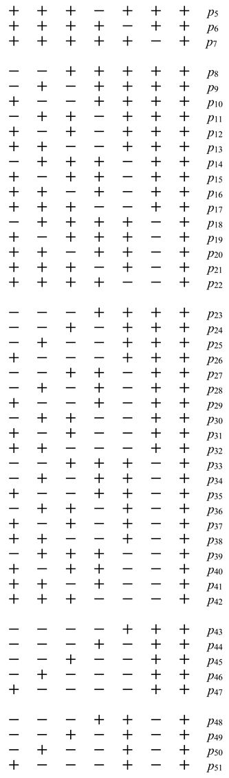
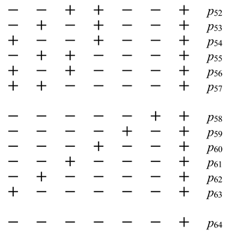
We define a special form of correlation in time series y(k), k = 1,…,N. The next state y(k+1) will depend on the current state y(k) and on the sequence of p signs of the previous increments: Δ(k-p-1),…., Δ(k), where Δ(k) = y(k) – y(k-1). This relationship is related to the assumed probability of the next increase or decrease. We use a different notation for the probabilities (i.e., p(i)) when the last increment was positive and a different notation (i.e., q(i)) for those when it was negative (see Figure 1), where i = 1, ..., 2p-1. This distinction will facilitate the introduction of the concepts of symmetric, asymmetric and antisymmetric persistence in time series. Figure 1a (Figure 1b) shows the case when the last increment is positive (negative), then the probability that the next increment will follow the trend is related to the probability given by the parameter p(k) (q(k)).
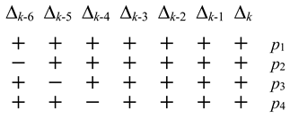
The number of all states for the p signs of the previous increments is 2p. In Appendix we present a list of all states with assigned probabilities p(k) (q(k)) for the case p = 7. The order determined by index k results from three adopted rules: the number of signs ‘minus’ (‘plus’) in the sequence; the moving of signs ‘minus’ (‘plus’) to the right; the last increment has a positive (negative) sign. Parameter p determines the order of persistence in our model.
2.2. Modified Discrete Langevin Model
The discrete version of the classical Langevin equation [11,12]
can describe an evolution of Markov (of order 1) series only. The deterministic drift term is given by the drift function a(y), the stochastic diffusion term by the diffusion function b(y) and the independent random variable ξk with normal density, Δ is the time step. In order to generalize the equation for finite-range correlated cases the additional factor is introduced to the diffusion term:
where the new function c(…) determines the sign of the term, therefore the noise is replaced by the absolute value of the noise |ξk|. Function c(…) depends on vector sk= [sk1, sk2, …, skp], the random scalar variable rk with uniform distribution in (0, 1) and the deterministic vector parameter D. Vector sk represents a pattern of signs of p previous increments i.e., sign(Δ(k-p-1)), …, sign( Δ(k)), before state y(k), (e.g., [+ − + + − − +] for p = 7) whereas D = [p(1), p(2), …p(2p-1), q(1), q(2), …, q(2p-1)] contains 2p persistence parameters. Function c(…) takes only two values 1 or -1. In each step the value of rk is drawn from the uniform distribution and ξk from the normal distribution. Let the pattern before y(k) be e.g., [+ − + + − − +] and the assumed probability of the pattern is p(40) (see list of patterns in Appendix), then when rk < p(40) function c(…) = 1, otherwise c(…) = - 1. For persistent series of order p the function is maintaining the tendency of increase (decrease) in the next step according to assumed vector parameter D. When all parameters p(i) and q(i) are greater than 0.5 ( lower than 0.5) the time series is persistent (antipersistent) and is Markovian for p(i) = q(i) = 0.5. If simultaneously there appear components of D greater and smaller than 0.5 the series has a mixed persistence. The case when p(i) = q(i) (p(i) = 1 - q(i)) for all i is called symmetric (antisymmetric) persistence. In other cases we have asymmetric persistence
Obviously, when all components of D are the same the p-persistent model is reduced to 1-persistent model [4] (let us note that the persistence parameter d in that paper is equal to 1-D).
2.3. The Hurst Exponent
The range of memory in our model is limited (in each step) to signs of p previous increments. The purpose of this subsection is to show how this property is represented by the Detrended Fluctuation Analysis which usually is used to estimation of the Hurts exponent [8,9]. The result of DFA is the fluctuation function F(n). If this function behaves as a power law in a certain range of n (in DFA procedure the profile of time series is cut into N/n segments of length n), the exponent is related to the Hurst exponent.
Three time series were generated using Eq. (2) with: a(y) = 0, b(y) = 1 (representing an analogue of the Brownian walk), persistence of order p = 1, p = 4, p = 7, and symmetric parameters p(k) = q(k) with values starting from a strong persistence 0.8 and gently decreasing with k to a Markovian value 0.5. Figure 2a–c show fluctuation functions obtained for this cases. Black line is related to the Hurst exponent H = 0.8. For larger values of n, the slope of the fluctuation function changes to a value corresponding to H = 0.5 (green line). We can observe that the crossover nc between the two scaling regimes (the long-range correlation regime and the uncorrelated behavior) increases with order of persistence p, from nc = 100 for p = 1 to nc = 500 for p = 7. For comparison, Figure 2d shows F(n) for the case of fractional Brownian motion with H = 0.8. Here the long-range correlation regime has a size comparable to the length of the generated time series.
2.4. Comparison with Fractional Brownian Motion
Fractional Brownian motion [13] was introduced as a generalization of Brownian motion for the case of long-range correlations. For this purpose, fractional integral was used, which involved taking into account the entire past of the process. Unlike our p-persistent model in which each state remembers only p previous increments, in fBm the memory includes all previous values of the process. Positive and negative correlations are symmetric in fBm which corresponds to symmetric persistence in our model. Let us treat the series generated by fBm with H = 0.7 as if it were generated by our 7-order persistent model, then the reconstruction of vector parameter D leads to values p(i) and q(i) shown in Figure 3. Since p(i) = q(i), i = 1,…, 64, this confirms the symmetry of persistence
in fBm. Moreover, Figure 3 shows how the memory built into fBm is expressed by the behavior of persistence parameters. In general their values are decreasing with increasing k but we notice a few jumps. Therefore, if we wanted to rely on fBm, we would have to renumber the parameters (in order to avoid these jumps) but there is no need to do this in present work.
3. Asymmetric Persistence
Asymmetric persistence means that all or only some of the parameters p(i) differ from the corresponding parameters q(i). Then the upward trend in time series differs from the downward trend. In this section, we present three examples illustrating the impact of asymmetric persistence on certain features of the generated time series.
In Example 1 we generate time series of length N = 106 using Eq. 2 with a(y) = 0, b(y) = 1, p = 7, time step Δ = 0.01 and persistence parameters in the following forms:
Values of the parameters start from 0.9 (0.6) and decrease with k to 0.5. By adopting a functional form of parameters, we avoid the tedious task of determining the value of each of the 128 persistence parameters. After applying DFA procedure, we obtain the fluctuation function F(n) shown in Figure 4a. In the first scaling regime (black line) the Hurst exponent H = 0.686 and then drop to H = 0.5 (green line). The procedure DFA does not take into account asymmetry of persistence and its result H = 0.686 is equal to an average value of p(k) + q(k).
In Example 2 we only change values of persistence parameters:
In this antisymmetric case the fluctuation function gives the Hurst exponent H = 0.5 (see Figure 4b, black and green line) what suggests that time series is uncorrelated. However, according to assumed values of parameters, the time series is strongly persistent in downward trend and strongly antipersistent in upward trend. This means that DFA may incorrectly recognize the level of correlation in time series where asymmetric correlations exist because actually it only finds their average effect.
In both of the above examples, the absence of a drift term (i.e., a(y) = 0) was assumed (like in free random walk) which means there were no potential V(y) of the drift force (where V’(y) = -a(y)) that would limit the dynamics of the process In Example 3 we introduce a simple quadratic potential V(y) = y2/2 (then a(y) = - y) but other assumptions are adopted from Example 2. The generated time series is stationary (unlike in Example 1 and 2). Its values cluster around y = - 3.56 (see Figure 5a) instead of y = 0 even though the minimum of the potential is at zero. According to a simple physical interpretation, the Langevin equation describes fluctuation of a particle in the potential well (see Figure 5b). The fluctuations are governed by the stochastic diffusion forces that interact with drift forces (potential). For the case of symmetric persistence the stochastic forces are amplified (weakened) by the action of persistent (antipersistent) trends but values of time series still are clustered around the minimum of the potential (see green distribution function f(y) in Figure 5b). Asymmetric persistence (e.g., as the one given by Eqs. (5) and (6)) leads to an asymmetry of stochastic forces and as a result it will cause a shift of the distribution function (see red distribution in Figure 6b).
4. Reconstruction of the Drift and Diffusion Functions from Time Series
For the case of the classical Langevin equation the procedure of reconstruction of the drift and diffusion functions (here we call it the standard procedure) was proposed in Ref. [10] and then developed in many papers [14,15,16,17]. However, for generalized non-Markov models the method fails. In papers [4,5] it was shown that for Langevin-type model with symmetric persistence the standard procedure leads to a wrong reconstruction of the drift function but to a good estimation of the diffusion function, therefore the new modified procedure was proposed. Unfortunately, for general asymmetric cases this procedure also fails.
In this chapter we will show the influence of various forms of persistence on the deformations of drift and diffusion functions reconstructed using the standard procedure. To this aim we assume three different cases of the functions:
however, these three examples have a common feature - the classical Langevin equation with these forms of functions generates stationary time series characterized by a Gaussian (or half-Gaussian) distribution function. By maintaining this type of uniformity, we avoid the influence of the form of the distribution function on our analysis.
4.1. Symmetric Persistence
We generate three sets of time series using Eq. (2) where drift and diffusion function are given by three cases M1 – M3. Each set consists of two time series; in one we assume the following symmetric form of persistence parameters:
and in the other the form
The order of persistence p = 7, time step Δ = 0.01 and the length of series is N = 2x10⁶. Applying the standard procedure [10] to the generated series, we obtain reconstructions of the drift functions, which differ significantly from the initial assumed forms in M1 – M3 (see Figure 6). However, the reconstruction of the diffusion function is correct (in accordance with the conclusions of Ref. [5]). Figure 6a suggests that the obtained deviations may be the result of rotation of the initial drift function, but in nonlinear cases we are dealing with a combination of rotation with additional slight deformation. The angle of ‘rotation’ of the drift function graph increases as the average value of p(k) + q(k) increases (which corresponds to the value of H estimated by DFA).
4.2. Antisymmetric Persistence
Here we also apply three cases M1 - M3, but each set consists of three time series because the following three antisymmetric forms of persistence parameters were assumed for them:
Figure 7 shows the reconstructed drift functions. With increasing value of p(1) in Eqs. (12) – (14) the graphs of drift functions are increasingly shifted from the graph of the initial function, however the transformation is not a pure translation. Moreover, in antisymmetric case also the diffusion functions b(y) are incorrectly reconstructed, although the deviations are less significant (see Figure 8). Particularly unsatisfactory, in the context of reconstruction, is the result of the DFA procedure, which gives an estimate of the Hurst exponent H ≈ 0.5 for all cases with antisymmetric persistence parameters (as shown in Section 3, DFA gives the average value of p(k) + q(k)). Thus, DFA treats antisymmetric cases as Markovian regardless of the level of persistence.
4.3. Asymmetric Persistence
In this subsection we assume two forms of persistence parameters that are neither symmetric nor antisymmetric, i.e.:
and:
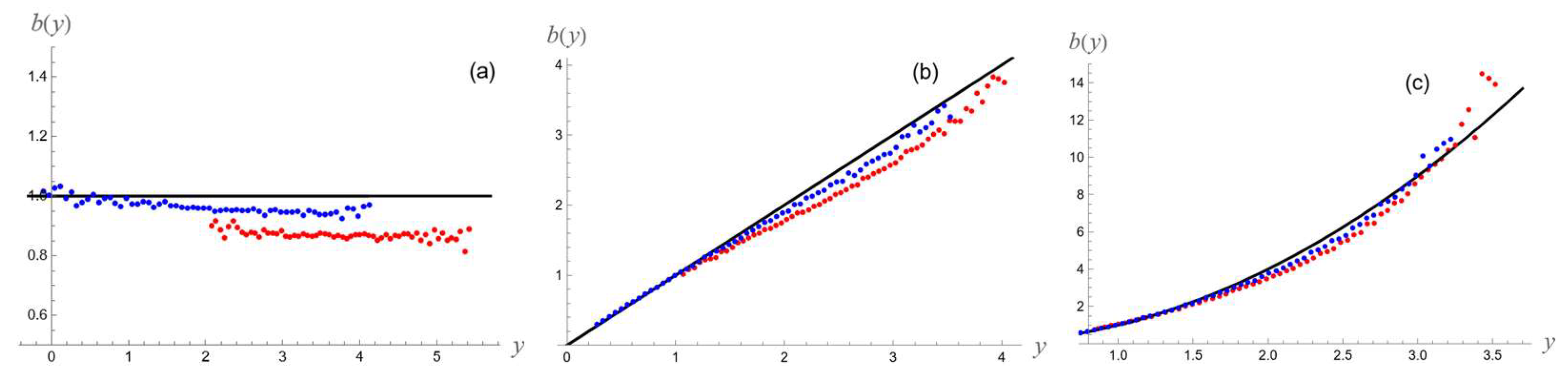
Parameters given by Eqs. (15), (16) mean strong upward persistence and weak downward persistence, while (18) indicates a downward antipersistent trend. The reconstructed drift functions (Figure 9) are significantly deviated from initial forms. The deviations are combinations of the transformations mentioned in the previous two subsections: ‘rotation’ and ‘translation’. Similarly to the antisymmetric case, the reconstructed diffusion functions differ from the initial functions, although the deviations are not so large (see Figure 10).
5. Discussion
The introduction of the concept of asymmetric persistence allows for a deeper analysis of time series and their more proper modeling. Hidden mechanisms in complex geophysical, biological or economic processes may be of a different nature when they lead to an upward trend than those which lead to a downward trend. Standard models assuming symmetry not only oversimplify the examined process but also do not provide the opportunity to identify these mechanisms. However, like most generalizations, the assumption of asymmetric persistence also leads to additional difficulties and challenges.
The present work concerns a stochastic time series model based on the Langevin equation with built-in finite-range persistence. Although an appropriate model was already derived in our paper [5], the procedure for its reconstruction from time series was tested only for symmetric persistence. Unfortunately, this procedure does not work in asymmetric cases. In the present paper, we re-analyze this p-order persistent model in the context of its application to time series in which asymmetric persistence may operate. We increased the memory length from p = 5 (in Ref. [5]) to p = 7, which resulted in a fourfold increase in the number of parameters. The comparison of this model with the fractional Brownian motion has shown that the persistence in the fractional model is symmetric. To make our model more similar to fBm, we should slightly change the order of persistence parameters in Appendix.
The next part of the work concerned the analysis of the effectiveness of standard procedures for the analysis of time series with asymmetric persistence and the reconstruction of the model from these data. The time series were generated by Eq. (2) assuming different forms of the drift and diffusion functions and persistence parameters.
The example of p-order persistent walk shows that the estimation of the Hurst exponent made by the DFA procedure may suggest misleading conclusions when we are dealing with asymmetric persistence. For example, for any antisymmetric persistence it gives the Markovian value H = 0.5. The explanation is quite simple - DFA gives the average result equal
By adding the potential the freedom of the persistent trend is limited and it complicates the dynamics of the process. The stochastic force associated with the trend competes with the drift force and the process may find a different steady state location. This causes a shift of the generated time series, which makes the reconstruction of the function a(y) very difficult. In the symmetric case there is no such shift and then the reconstruction procedure proposed in Ref. [5] works well. However, for asymmetric cases a new procedure must be developed.
From the examples analyzed in Section 4 we can conclude that the reconstructions of drift function a(y) obtained by the standard procedure [10] are very different from the initial function. For symmetric persistence the main transformation of drift function is rotation, for antisymmetric it is shift and for more general asymmetric cases it is a combination of rotation and shift. In addition, the functions experience another, much smaller shape deformation. It should be emphasized that asymmetric persistence also causes incorrect reconstructions of the diffusion function b(y) obtained from the standard method. (only in the symmetric case the reconstruction of b(y) is correct).
Referring to our reconstruction procedure of p-persistent model [5] the basic problem caused by asymmetry of persistence is the significant shift of the reconstructed a(y) relative to the initial drift function. When dealing with a real time series, we do not know whether the potential is shifted or whether the shift is a result of asymmetric persistence in the process (moreover both of these factors may act simultaneously). In fact, this is the main reason for the failure of the reconstruction procedure proposed in Ref. [5]. Rotations do not cause as big changes as shifts and the procedure was able to identify them. Therefore, developing a new procedure for the model with asymmetric persistence is a big challenge. The results of this work should help in this task because they show problems that need to be solved.
Supplementary Materials
The following supporting information can be downloaded at the website of this paper posted on Preprints.org.
Author Contributions
Conceptualization, Z.C.; methodology, Z.C.; software, Z.C.; formal analysis, Z.C.; investigation, Z.C.; writing—original draft preparation, Z.C.; writing—review and editing, Z.C.; visualization, Z.C.; project administration, Z.C.; funding acquisition, Z.C. All authors have read and agreed to the published version of the manuscript.
Funding
This research was funded in part by National Science Centre, Poland, Contract No. UMO-2022/45/B/ST10/01621.
Data Availability Statement
The data that support the findings of this study are available from the corresponding author upon reasonable request.
Conflicts of Interest
The authors declare no conflicts of interest.
Appendix A
Here we present a list of patterns symbolizing the signs of seven previous increments with the parameters p(k) assigned to them. The list for parameters q(k) is analogous, one only need to replace: p by q, "+" by "-" and "-" by "+".
References
- Franses, P.H.; Paap, R. Modelling asymmetric persistence over the business cycle, Econometric Institute Research Papers, 1998, (No. EI 9852). Retrieved from http://hdl.handle.net/1765/1525.
- Rossetto, V. The one-dimensional asymmetric persistent random walk, J. Stat. Mech., 2018, 043204. [CrossRef]
- Czechowski, Z.; Telesca, L. Construction of A Langevin model from time series with a periodical correlation function: Application to wind speed data, Phys. A 2013, 392, 5592-5603. [CrossRef]
- Czechowski, Z. Reconstruction of the modified discrete Langevin equation from persistent time series. Chaos 2016, 26, 053109. [CrossRef]
- Czechowski, Z. Discrete Langevin-type equation for p-order persistent time series and procedure of its reconstruction. Chaos, 2021, 31, 063102. [CrossRef]
- Kubo, R. The Fluctuation-Dissipation Theorem. Rep. Prog. Phys. 1966, 29, 255-284. [CrossRef]
- Mainardi, F.; Mura, A.; Tampieri, F. Brownian motion and anomalous diffusion revisited via a fractional Langevin Equation. Mod. Probl. State Phys. 2009, 8, 3 (2009); E-print http://arxiv.org/abs/1004.3505.
- Kantelhardt, J.W; Koscielny-Bunde, E.; Rego, H.H.A.; Havlin, S.; Bunde, A. Detecting long-range correlations with detrended fluctuation analysis. Physica A 2001, 295, 441- 454.
- Kantelhardt, J.W. Fractal and multifractal time series. arXiv: 2008, 0804.0747v1, 1-59. [CrossRef]
- Siegert, S; Friedrich, R.; Peinke, J. Analysis of data sets of stochastic systems. Phys. Lett. A 1998, 243, 275-280. [CrossRef]
- Grasman, J.; van Herwaarden; O. A. Asymptotic Methods for the Fokker-Planck Equation and the Exit Problem in Applications. Springer-Verlag, Berlin, Germany, 1999.
- Oksendal, B. Stochastic differential equations: an introduction with applications; Springer-Verlag, Berlin, Germany, 1998.
- Mandelbrot, B.B.; Van Ness, J.W. Fractional Brownian Motions, Fractional Noises and Applications. SIAM Rev. 1968, 10, 422-437. [CrossRef]
- Sura, P.; Barsugli, A note on estimating drift and diffusion parameters from timeseries. J. Phys. Lett. A 2002, 305, 304-311. [CrossRef]
- Gottschal, J.; Peinke, J. On the definition and handling of different drift and diffusion estimates. New J. Phys. 2008, 10, 083034. [CrossRef]
- Anteneodo, C.; Riera, R. Arbitrary order corrections for finite-time drift and diffusion coefficients. Phys. Rev. E 2009, 80, 031103. [CrossRef]
- Friedrich, R.; Peinke, J.; Sahimi, M.; Reza Rahimi Tabar, M. Approaching complexity by stochastic methods: From biological systems to turbulence. Physics Reports 2011, 506(5), 87–162. [CrossRef]
Figure 1.
Ilustration of the p-order persistence concept (for p = 7); y(k-7),..., y(k-1) - values of the seven states of the time series preceding the current state y(k); symbols + and - denote the signs of the seven previous increments; red arrows – next possible increment. (a) Case where the last increment has the positive sign, then the sign of next stochastic increment will also be positive with probability p(15) and negative with probability 1 - p(15); (b) Case where the last increment has the negative sign, then the sign of next stochastic increment will also be negative with probability q(50) and positive with probability 1 - q(50). The values of p(15) and q(50) depend on the sequence of seven signs of previous increments that are listed in Appendix.
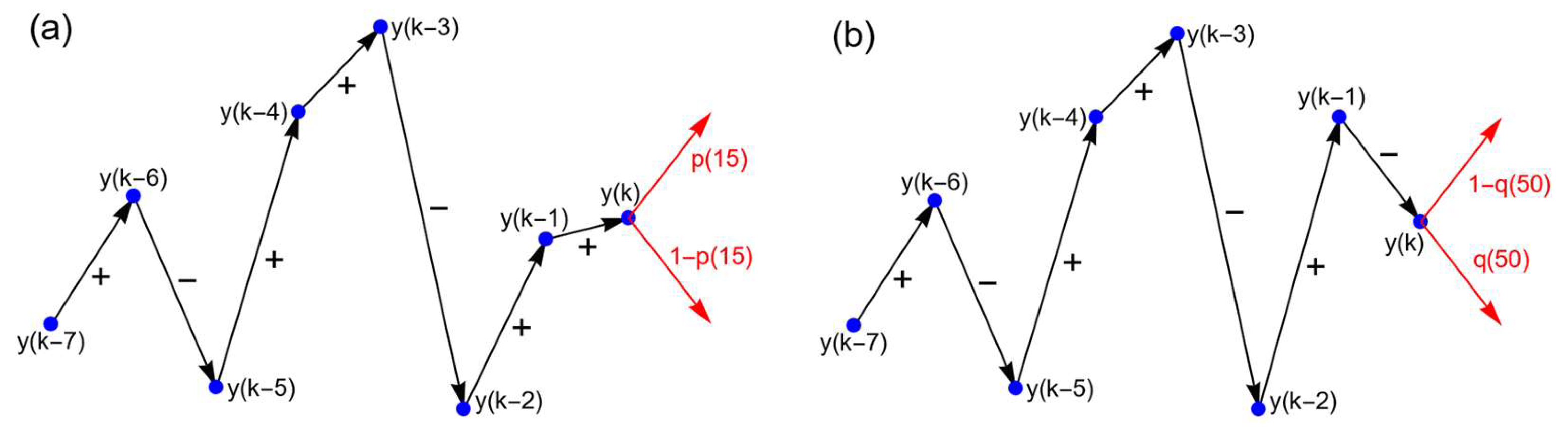
Figure 2.
Fluctuation functions F(n) obtained from p-order persistent time series generated by Eq. (2) with a(y) = 0, b(y) = 1 and symmetric parameters, p(k) = q(k). (a) Case p = 1; (b) p = 4; (c) p = 7; (d) F(n) is obtained from fBm with H = 0.8. Black line represents H = 0.8, green line: H = 0.5.
Figure 2.
Fluctuation functions F(n) obtained from p-order persistent time series generated by Eq. (2) with a(y) = 0, b(y) = 1 and symmetric parameters, p(k) = q(k). (a) Case p = 1; (b) p = 4; (c) p = 7; (d) F(n) is obtained from fBm with H = 0.8. Black line represents H = 0.8, green line: H = 0.5.
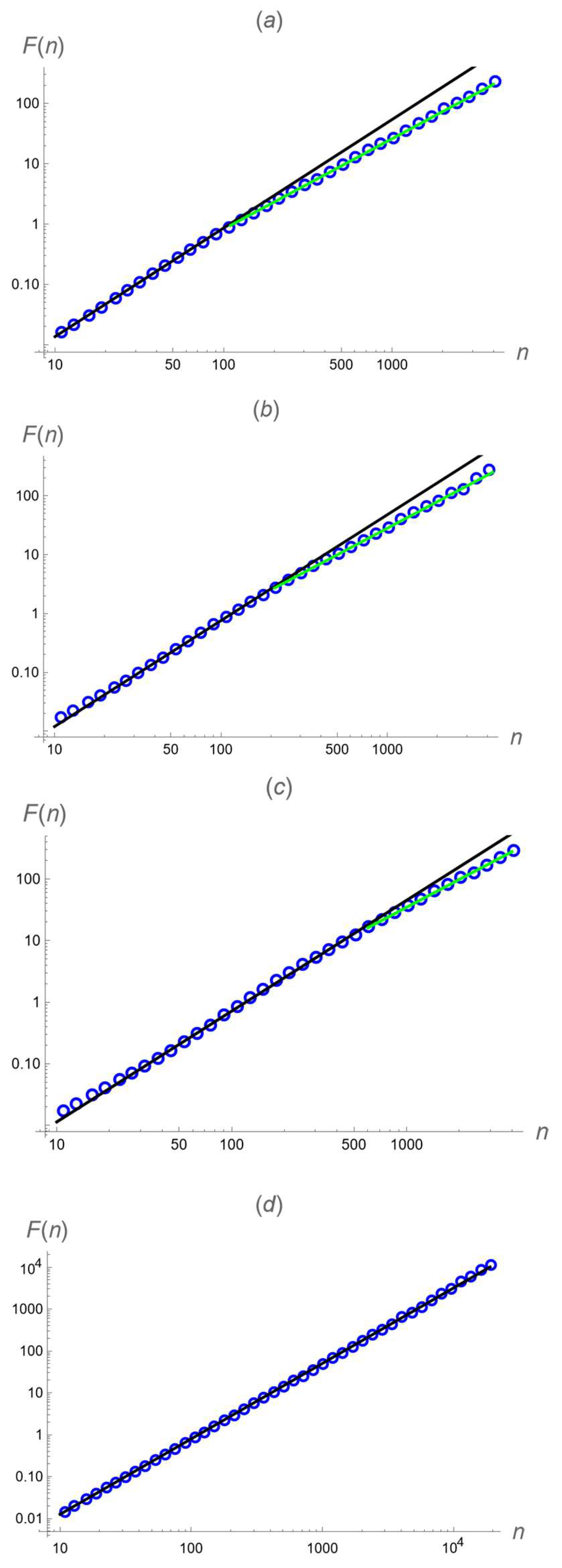
Figure 3.
Persistence parameters p(k) (red points) and q(k) (black +) reconstructed from fBm with H = 0.7. .
Figure 3.
Persistence parameters p(k) (red points) and q(k) (black +) reconstructed from fBm with H = 0.7. .
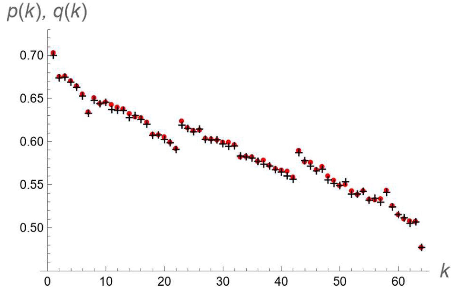
Figure 4.
Fluctuation functions F(n) obtained from p-order persistent time series generated by Eq. (2) with a(y) = 0, b(y) = 1. (a) Case with asymmetric parameters given by Eqs. (3) and (4). Black line represents H = 0.686, green line: H = 0.5. (b) Case with antisymmetric parameters given by Eqs. (5) and (6). Black and green lines represent H = 0.5.
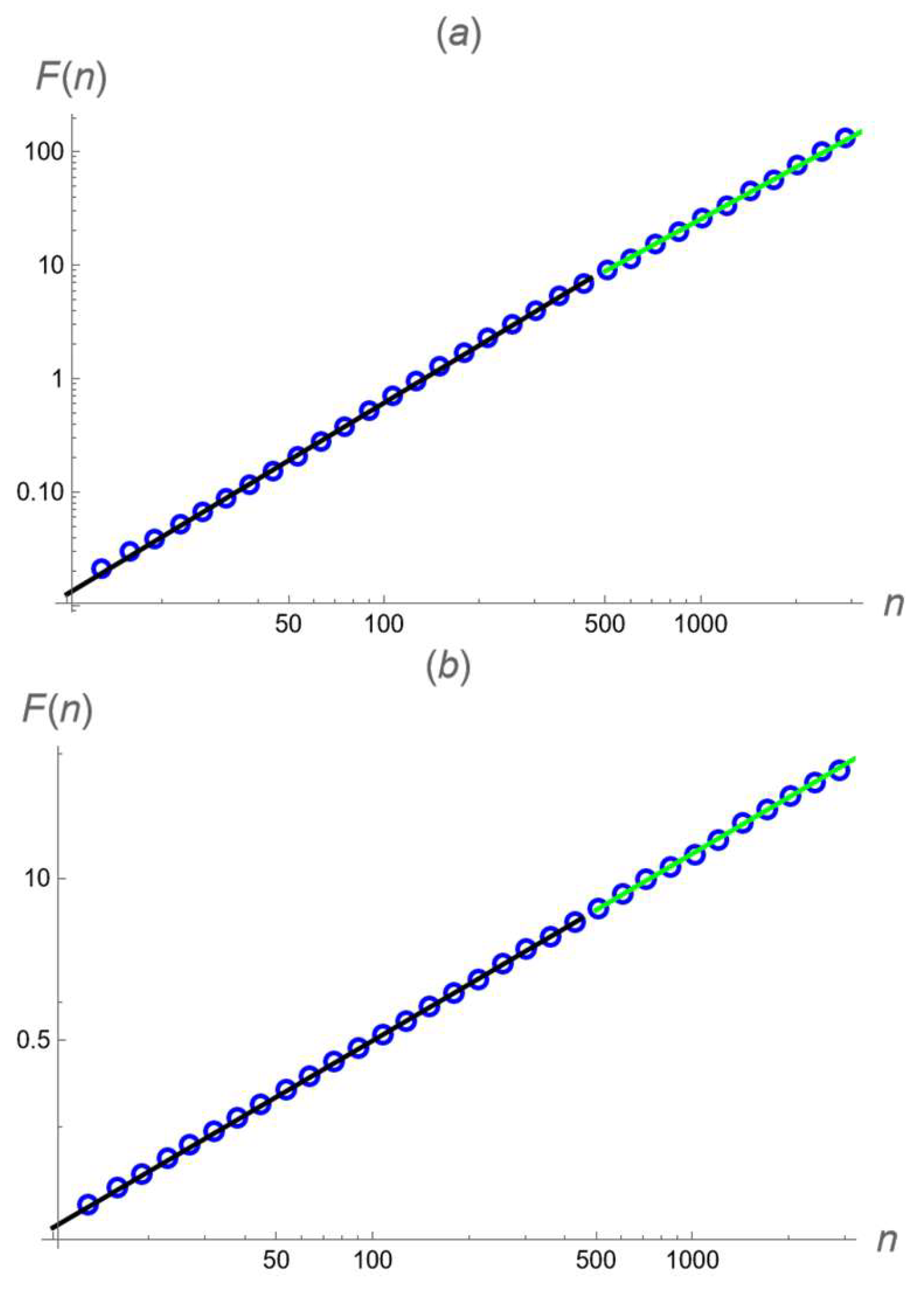
Figure 5.
(a) Time series generated by Eq. (2) with a(y) = - y, b(y) = 1 and antisymmetric parameters, Eqs. (5) and (6). (b) Potential V(y) (black graph), distribution function f(y) (red graph) of time series shown in plot (a). For a comparison the green graph represents the distribution function for a symmetric case.
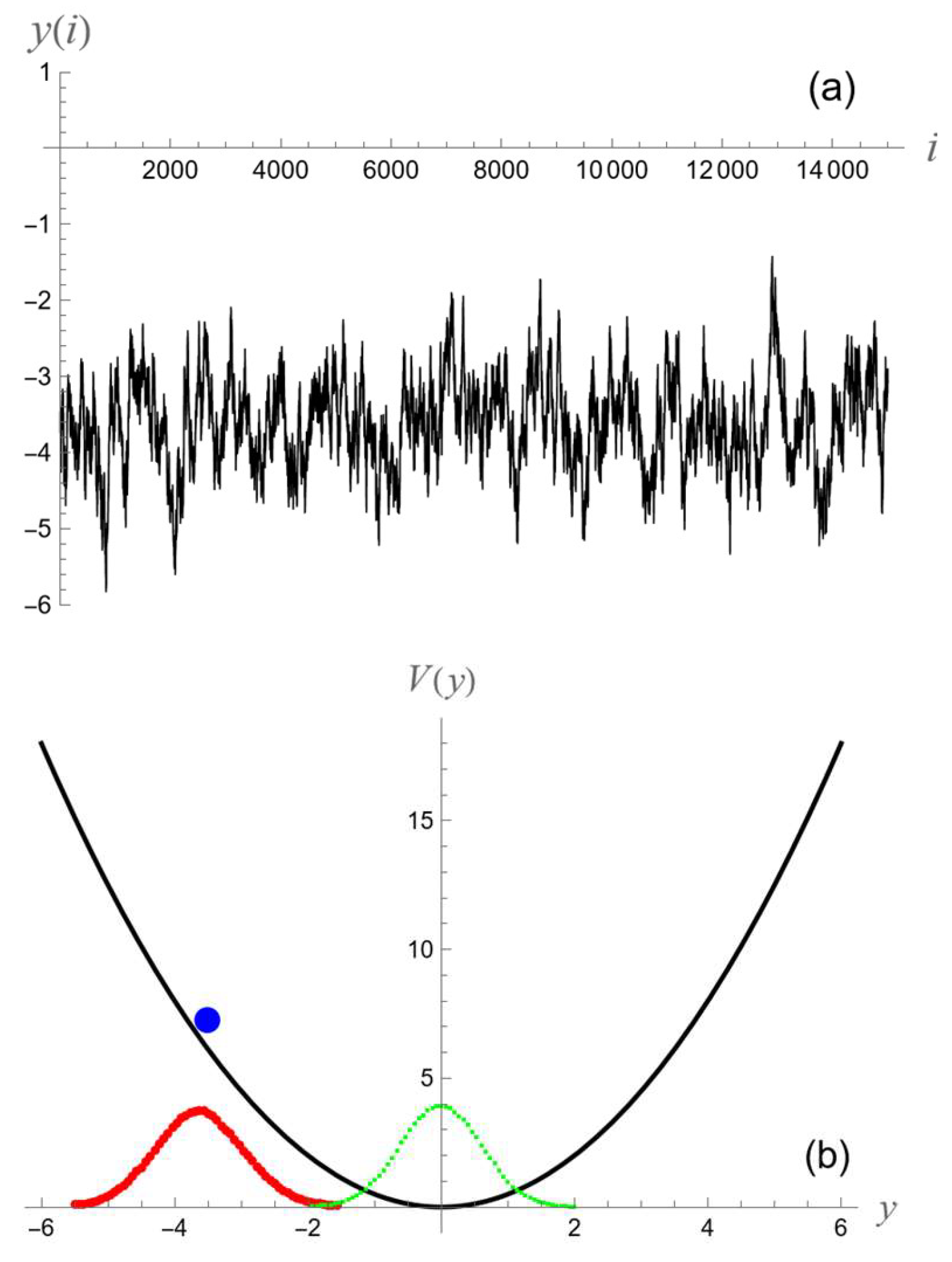
Figure 6.
Standard procedure reconstructions of drift functions from time series generated by Eq. (2) for two symmetric forms of persistence parameters given by Eq. (10) (blue points) and Eq. (11) (red points). (a) Case M1; (b) case M2; (c) case M3. Black graphs represent the initial forms of a(y).
Figure 6.
Standard procedure reconstructions of drift functions from time series generated by Eq. (2) for two symmetric forms of persistence parameters given by Eq. (10) (blue points) and Eq. (11) (red points). (a) Case M1; (b) case M2; (c) case M3. Black graphs represent the initial forms of a(y).
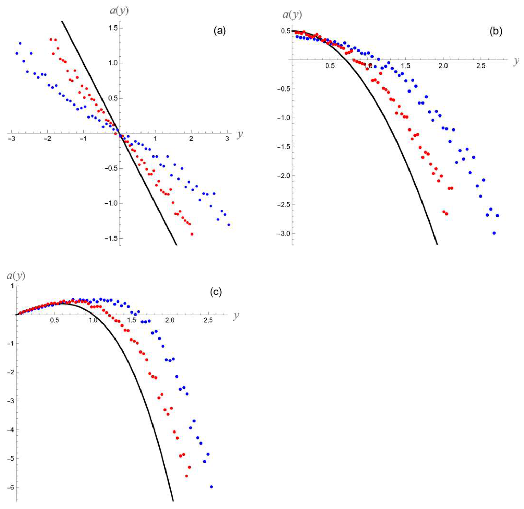
Figure 7.
Standard procedure reconstructions of drift functions from time series generated by Eq. (2) for three antisymmetric forms of persistence parameters given by Eq. (12) (blue points), Eq. (13) (green points) and Eq. (14) (red points). (a) Case M1; (b) case M2; (c) case M3. Black graphs represent the initial forms of a(y).
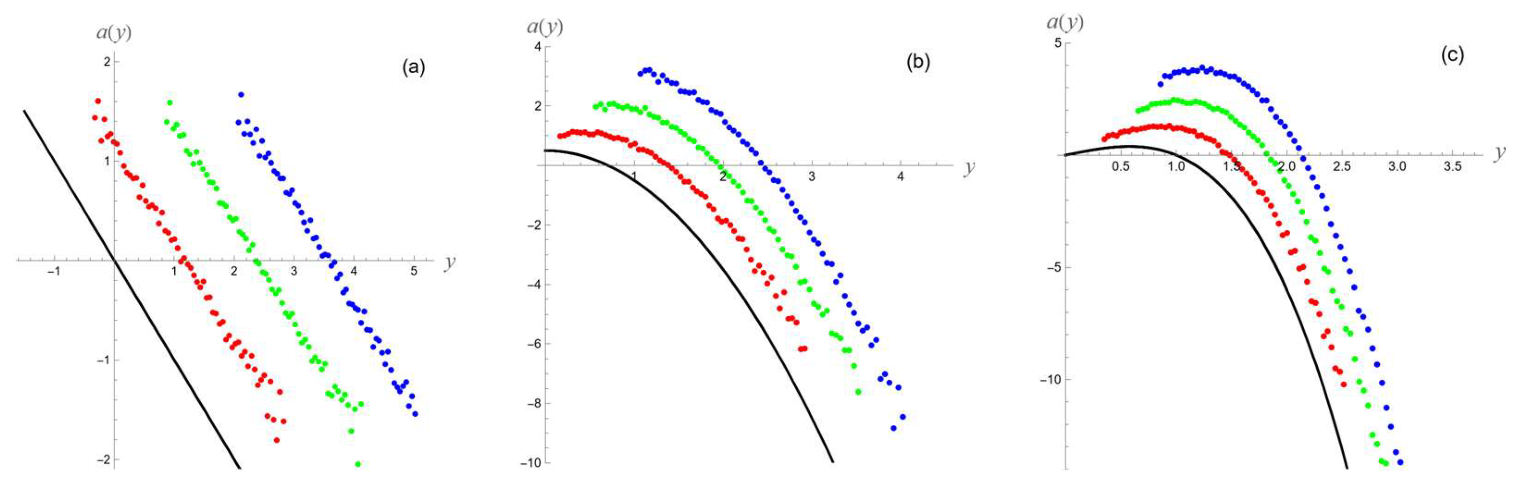
Figure 8.
Standard procedure reconstructions of diffusion functions from time series generated by Eq. (2) for the antisymmetric form of persistence parameters given by Eq. (12) (blue points). (a) Case M1; (b) case M2; (c) case M3. Black graphs represent the initial forms of b(y).
Figure 8.
Standard procedure reconstructions of diffusion functions from time series generated by Eq. (2) for the antisymmetric form of persistence parameters given by Eq. (12) (blue points). (a) Case M1; (b) case M2; (c) case M3. Black graphs represent the initial forms of b(y).
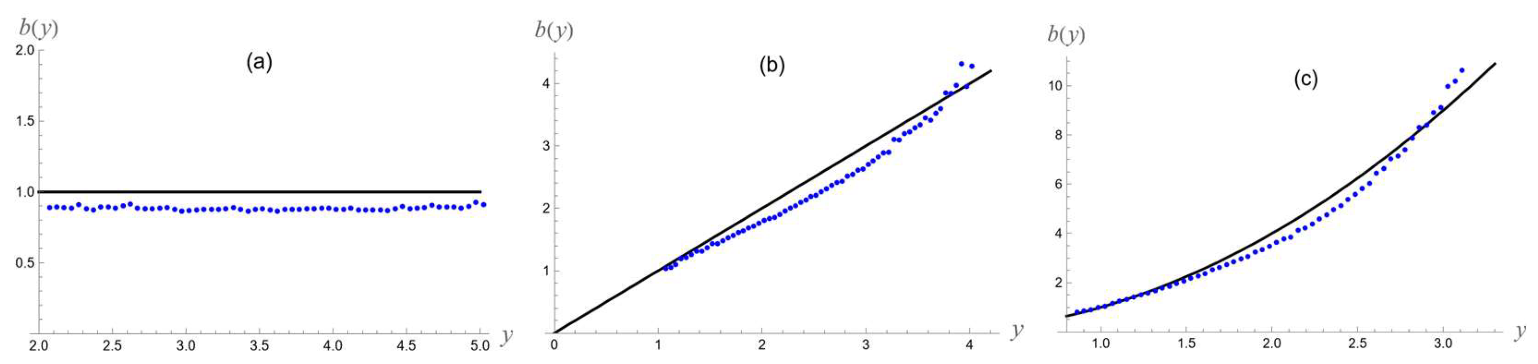
Figure 9.
Standard procedure reconstructions of drift functions from time series generated by Eq. (2) for two asymmetric forms of persistence parameters given by Eqs. (15), (16) (blue points) and Eqs. (17), (18) (red points). (a) Case M1; (b) case M2; (c) case M3. Black graphs represent the initial forms of a(y).
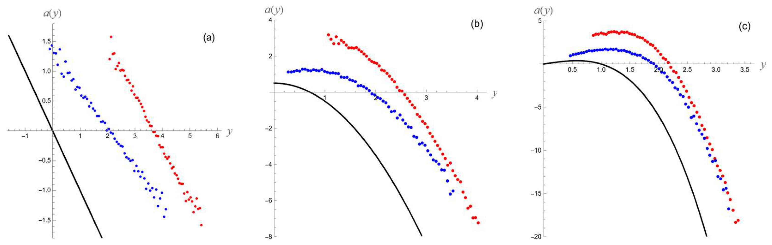
Figure 10.
Standard procedure reconstructions of diffusion functions from time series generated by Eq. (2) for two asymmetric forms of persistence parameters given by Eqs. (15), (16) (blue points) and Eqs. (17), (18) (red points). (a) Case M1; (b) case M2; (c) case M3. Black graphs represent the initial forms of b(y).
Disclaimer/Publisher’s Note: The statements, opinions and data contained in all publications are solely those of the individual author(s) and contributor(s) and not of MDPI and/or the editor(s). MDPI and/or the editor(s) disclaim responsibility for any injury to people or property resulting from any ideas, methods, instructions or products referred to in the content. |
© 2024 by the authors. Licensee MDPI, Basel, Switzerland. This article is an open access article distributed under the terms and conditions of the Creative Commons Attribution (CC BY) license (http://creativecommons.org/licenses/by/4.0/).
Copyright: This open access article is published under a Creative Commons CC BY 4.0 license, which permit the free download, distribution, and reuse, provided that the author and preprint are cited in any reuse.


