Submitted:
04 December 2024
Posted:
09 December 2024
You are already at the latest version
Abstract
This paper provides a comprehensive review of uncertainty quantification (UQ) methods and their applications in CFD aerodynamics. The review begins by discussing the various sources of uncertainty in CFD simulations, highlighting their impact on aerodynamic predictions. It then explores a range of UQ methods, including non-probabilistic, probabilistic, and Bayesian approaches, detailing their strengths and limitations in the context of aerodynamics. The paper further examines the application of these methods to real-world CFD problems, showcasing their effectiveness in addressing uncertainties inherent in aerodynamic simulations. Additionally, challenges and limitations of applying UQ techniques in CFD aerodynamics are critically evaluated. The review concludes by outlining potential future research directions aimed at advancing UQ methodologies and their integration into CFD-based aerodynamic design and analysis. Key takeaways from the study are presented to provide a foundation for further developments in this important area of research.
Keywords:
UQ
; Aerodynamics
; CFD
1. Introduction
Before quantifying uncertainty, it is essential to distinguish it from "errors," as the two are often confused. According to the AIAA standard definition [1], uncertainty is “a potential deficiency in any phase or activity of the modeling process that arises from a lack of knowledge.” This uncertainty typically stems from gaps in understanding physical models or input parameters, leading to unreliable simulations. In contrast, errors are defined as “a recognizable deficiency in any phase or activity of modeling and simulation that is not due to a lack of knowledge.” Errors, therefore, result from identifiable issues that can be diagnosed and corrected.
With these definitions in mind, this study focuses on uncertainty quantification (UQ) [2], which involves characterizing input uncertainties, propagating them through the model or system, and performing statistical or interval assessments of the resulting outputs. In short, it assesses how uncertainties and assumptions affect the model’s predictions.
These uncertainties are generally categorized into two types [3]:
- Aleatory uncertainty (irreducible uncertainty): This type is related to inherent variability in the system or its environment, such as material properties, manufacturing tolerances, or boundary conditions. Aleatory uncertainty cannot be reduced, but it can be addressed through additional experiments to gather more data or by using probabilistic methods
- Epistemic uncertainty (reducible uncertainty): This type arises from a lack of knowledge about the physical model itself, often stemming from assumptions or simplifications in the model’s formulation (e.g., turbulence models, periodicity, or steady-state conditions). Unlike aleatory uncertainty, epistemic uncertainty can be reduced by conducting more experiments and using the results to refine and improve the underlying physical models.
The inclusion of uncertainty in the design process has shifted traditional methods, which relied on safety margins and knockdown factors, toward more advanced approaches like robust design and reliability-based design. Robust design aims to create solutions that are relatively insensitive to small variations in uncertain variables, ensuring consistent performance under variability. Reliability-based design, on the other hand, ensures that the probability of failure remains below an acceptable threshold, emphasizing both safety and reliability.
These new approaches offer several advantages over traditional methods [4]. They improve confidence in analysis tools, reduce design cycle time, lower costs and risks, and enhance system performance while meeting reliability requirements. Additionally, they lead to more robust designs that can perform effectively under off-nominal conditions.
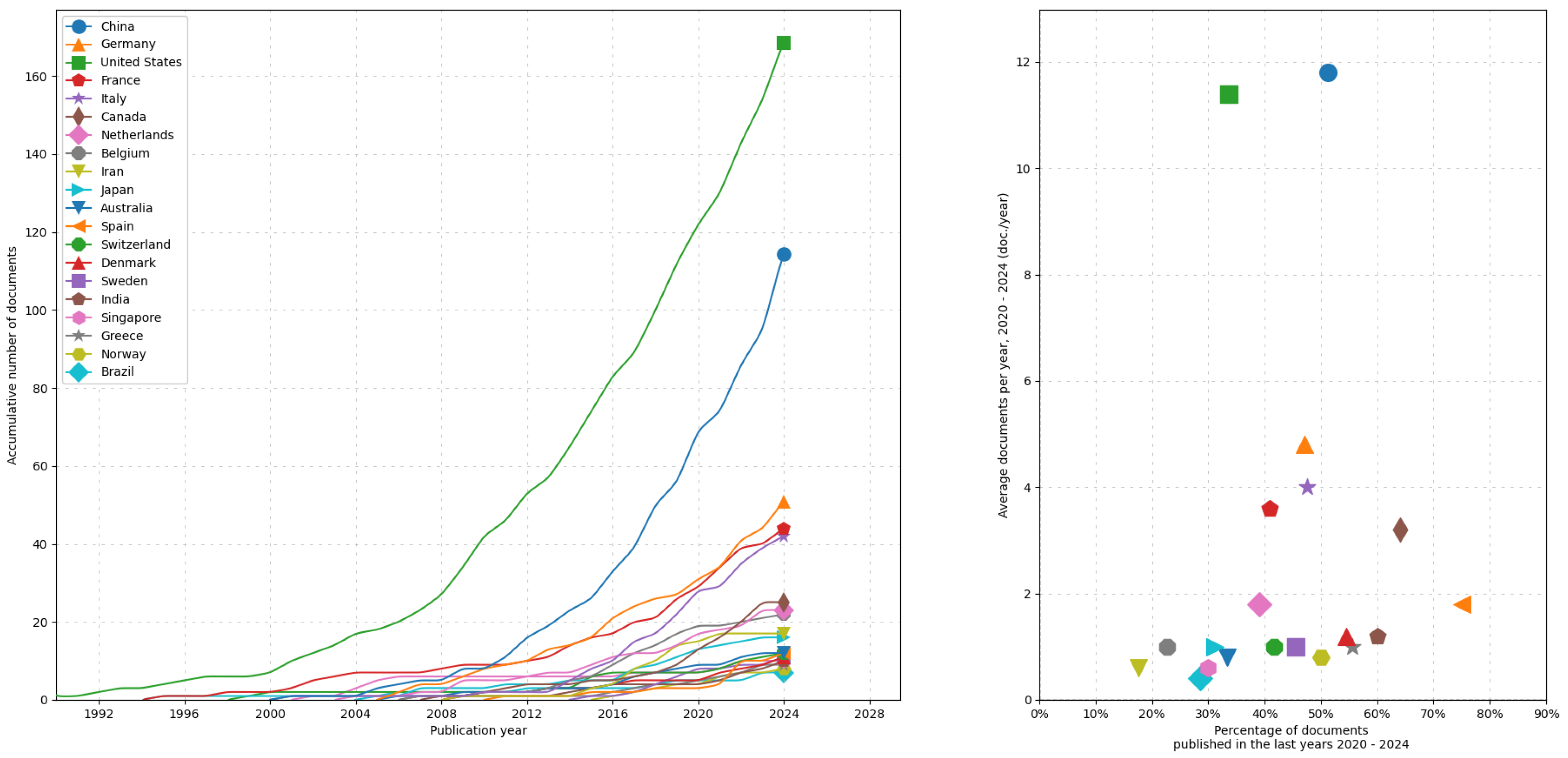
As part of a preliminary bibliometric study, we conducted an analysis to better understand the evolution and key trends in the field of UQ applied to CFD. The figures presented provide an overview of the most relevant keywords in the literature and the geographical distribution of contributions across different countries over time. Figure 1 (left) shows a histogram highlighting the frequency of key terms found in UQ-CFD publications, while Figure 1 (right) illustrates a word cloud that emphasizes the most prominent concepts. Additionally, Figure 2 examines the temporal trends in the contributions from various countries, shedding light on the global development of this field.
To illustrate the importance of these uncertainties, although they will be detailed in later sections, we provide a few typical examples of aleatory uncertainty effects. For instance, uncertainty in inlet conditions, such as inlet temperature in the high-pressure stage of a turbine, can lead to significant variations —up to 60% in the Nusselt number on the pressure side [6]. Similarly, Dam et al. (2024) [7] found that small modifications (1% chord) in the trailing edge can increase mechanical and thermal stresses, particularly in the hub and shroud regions.
Salvadori, Insinna, and Martelli [8] studied the interaction between combustor and turbine components, identifying a residual swirl from the combustor that altered the stagnation point location on the high-pressure vane by as much as 4% of the chord. In the context of wind turbine airfoils, Marepally et al. (2022) [9] showed that uncertainty in lift coefficients and lift-to-drag ratios becomes particularly significant near the stall region. A 5% deviation in geometric parameters caused about a 3% deviation in these quantities near the operating point, with uncertainties increasing from around 5% to more than 10% for thinner and thicker airfoils, respectively, near the stall region.
Regarding epistemic uncertainties, a typical example is found in Reynolds-Averaged Navier–Stokes (RANS) models [10]. These models are limited in replicating certain characteristics of turbulent flows due to inherent simplifications, such as the assumption that the Reynolds stress tensor can fully describe the turbulent flow field. Other simplifications include the eddy viscosity hypothesis, which assumes Reynolds stress anisotropy is proportional to the mean rate of strain, and the gradient diffusion hypothesis for modeling turbulent transport. While these assumptions may be relatively accurate for simpler flows, they can introduce significant discrepancies in more complex turbulent flows, especially those involving mean rotation effects, swirl, or strong streamline curvature, where the fidelity of linear eddy-viscosity-based closures often falls short.
This review is structured to provide a comprehensive overview of uncertainty quantification (UQ) methods and their applications in CFD aerodynamics, along with insights into potential future research directions. In Section 2, we discuss the various sources of uncertainty in CFD aerodynamics. Section 3 explores the different UQ methods, including non-probabilistic, probabilistic, and Bayesian approaches. Section 4 addresses the challenges and limitations associated with UQ in this field. Section 5 outlines future directions for advancing UQ in CFD aerodynamics.
2. Uncertainty Sources in CFD Aerodynamics
In aerodynamics, the presence of various uncertainties can significantly affect the accuracy and reliability of both simulations and test. These uncertainties stem from multiple factors, including variations in geometry, boundary and initial conditions, model assumptions, and experimental measurements. A thorough understanding of these sources is crucial for improving model fidelity and predictive capability. In this section, we outline the key sources of uncertainty and their impact.
2.1. Geometric Uncertainty
Geometric uncertainty in CFD aerodynamics arises from several factors, including manufacturing tolerances, surface roughness, and operational deformations. These uncertainties introduce variability into the physical geometry of aerodynamic components, leading to discrepancies between simulation predictions and real-world performance. Managing these uncertainties is essential, as even small deviations from the ideal geometry can have significant effects on aerodynamic characteristics such as lift, drag, and overall efficiency.
One of the primary sources of geometric uncertainty is manufacturing variability. For example, slight deviations in the shape of an aircraft wing or imperfections in surface quality can lead to noticeable differences in aerodynamic behavior. Zhang et al. (2021) demonstrated the significant effect of surface roughness and manufacturing tolerances on drag predictions during wind tunnel testing of airfoils, showing how these uncertainties can alter performance estimates [11]. Similarly, Wu et al. (2018) investigated turbine blade performance and found that small geometric deviations from the nominal design could cause notable changes in lift and drag, highlighting the importance of precise manufacturing [12].
Manufacturing errors and in-service degradation also play a key role in geometric uncertainty. Over time, components such as gas turbines experience wear and tear that leads to deviations from their original geometry, which can negatively impact performance. Lange et al. (2020) explored the impact of 18 geometric uncertainty variables in a high-pressure compressor blade and found that the leading-edge thickness was the most influential factor affecting efficiency [13]. Further emphasizing the importance of key geometric parameters, Wang et al. (2023) showed that, under near-stall conditions, the blade tip leading-edge radius and tip thickness were the dominant factors influencing efficiency deviation. These parameters accounted for up to 54% of the total efficiency variation, underscoring the need for strict control over these features during manufacturing [14].
Another significant source of geometric uncertainty stems from operation, such as aeroelastic deformation. This is particularly challenging in aerospace applications where structures, like wings, experience dynamic forces that can alter their shape in real time. Righi, Carnevali, and Ravasi (2021) explored this phenomenon by studying flutter speed and found a broad confidence interval, with variability on the same order of magnitude as differences between lower and higher fidelity models. This indicates how unpredictable aeroelastic deformations can be, further complicating geometric uncertainty management [15,16].
Geometric uncertainties are especially difficult to measure and predict under real operational conditions. For instance, wing flexing during flight introduces deformations that challenge the accuracy of CFD simulations. To address this, probabilistic approaches can be used to model a range of geometric configurations and assess their impact on simulation outcomes. By incorporating these probabilistic techniques, engineers could better capture the influence of geometric variability and improve the robustness of their aerodynamic predictions.
2.2. Boundary and Initial Conditions
Boundary and initial condition uncertainties are key contributors to variability in CFD simulations, arising from fluctuations in external environmental and operating conditions. These uncertainties encompass factors such as wind speed, temperature, pressure, and turbulence intensity, all of which can vary during operation and significantly affect the accuracy of simulations. In complex aerodynamic flows, the sensitivity of the flow field to these parameters is particularly pronounced, making it essential to carefully quantify and account for their uncertainties during CFD analysis.
For instance, Araya et al. (2021) explored the impact of boundary condition uncertainties in CFD simulations of wind turbines. Their study revealed that even small variations in wind speed and direction could lead to substantial changes in predicted power output and the loading on turbine blades, underscoring the importance of accurately modeling external environmental conditions in wind energy applications [17]. Similarly, boundary condition uncertainties play a significant role in external aerodynamic simulations, such as vehicle design, where variations in temperature and humidity can alter the performance predictions of the vehicle under different environmental conditions.
The effect of turbulence intensity and environmental fluctuations on low Reynolds number aerodynamic designs has also been highlighted. García-Gutiérrez et al. (2020) identified how turbulence level fluctuations impact the optimal design of low Reynolds propellers and the performance of high-altitude airships. Their findings showed that turbulence significantly influences the aerodynamic performance of these systems, making it a crucial factor in their design optimization processes [18,19].
In the context of turbomachinery, uncertainty in operational conditions has attracted growing attention. For example, Tang et al. (2020) investigated the effects of stochastic operational conditions such as exhaust pressure, inlet flow, rotor speed, and mechanical vibration on the performance of centrifugal compressors. Their results demonstrated that these fluctuating conditions introduce variability in performance parameters, complicating the prediction of compressor behavior under real-world operating conditions [20]. Gopinathrao et al. (2009) utilized the non-intrusive probability collocation method (NIPRC) to analyze how variations in inlet total pressure affected the pressure ratio and efficiency of NASA Rotor 37, highlighting the sensitivity of turbomachinery performance to boundary condition uncertainties [21]. Similarly, Wang et al. (2009) examined the influence of random outlet static pressure on NASA Rotor 37, showing that robust design methods can mitigate the rapid decline in efficiency at off-design conditions, particularly at the choked flow point [22].
In supersonic flow applications, boundary condition uncertainties become even more critical. Lu et al. (2022) studied the influence of freestream parameters such as velocity, static pressure, and temperature on fin-plate configurations in supersonic flow. They found that uncertainties in these flow parameters, along with geometric variations in fin angles, could lead to significant deviations in heat transfer and pressure predictions on the bottom plate, with heat transfer uncertainty exceeding 30% in some cases [23]. Their study revealed that freestream velocity, pressure, and fin angle were the primary contributors to uncertainty, whereas wall temperature had a negligible effect.
2.3. Model Uncertainty
Model uncertainty in CFD arises from the inherent approximations and assumptions made in mathematical models used to simulate complex physical phenomena. This type of uncertainty has a significant impact on the accuracy of aerodynamic predictions, particularly in intricate flow regimes. One of the primary sources of model uncertainty stems from turbulence modeling, as the chaotic and multiscale nature of turbulence is challenging to fully capture with simplified models.
The widely used Reynolds-Averaged Navier–Stokes (RANS) equations are a prime example, as they rely on various assumptions, such as the eddy viscosity hypothesis, to model turbulent flows. These assumptions may work well for certain flow regimes but often fail to accurately capture anisotropic turbulence effects present in flows with strong curvature, swirl, or rotation. The assumption of linear eddy viscosity in particular limits the ability of RANS models to predict flows with significant anisotropic turbulence, leading to inaccuracies in the flow field predictions [24]. Numerous studies have documented these limitations. For instance, Slotnick et al. (2014) provided a comprehensive review of CFD applications in aerospace, noting the critical challenges posed by turbulence modeling [25]. Ghosal (1996) also highlighted the epistemic uncertainties introduced by turbulence models, which impact the prediction of complex flows [26]. Pope (2000) emphasized the inherent uncertainties in turbulence models and underscored the need for more rigorous methods to quantify and address these uncertainties [27].
More advanced turbulence models, such as Large Eddy Simulation (LES), address some of the shortcomings of RANS by resolving larger turbulent structures. However, LES still relies on subgrid-scale (SGS) models to account for the effects of smaller, unresolved turbulent eddies. The choice of SGS model can introduce additional uncertainty, as different models provide varying levels of accuracy depending on flow conditions. For example, the commonly used Smagorinsky model is sensitive to both the selected model parameters and the specific characteristics of the flow, which can affect the reliability of the results [28]. Furthermore, the grid resolution plays a critical role in LES accuracy, as finer grids resolve more turbulent scales, but at a higher computational cost. Despite these refinements, LES simulations can still diverge from experimental results due to uncertainties in SGS models and the stochastic nature of turbulence itself [27].
Beyond RANS and LES, hybrid models like Detached Eddy Simulation (DES) and Reynolds Stress Models (RSM) have been developed to address some of the uncertainties in traditional approaches. DES combines elements of RANS and LES, while RSM directly models the Reynolds stress tensor to better capture the anisotropic nature of turbulence. However, these methods also carry their own uncertainties, especially regarding parameterization and the transition between different flow regimes. Understanding these uncertainties is essential for producing reliable aerodynamic designs.
Other numerical techniques, such as panel methods, which are often used in inviscid flow simulations, also introduce model uncertainty. These methods approximate the flow field by discretizing surfaces into panels, which inherently limits their precision, especially near solid boundaries where the flow becomes more complex. The distribution of panels, if inadequate, can lead to substantial errors in the predicted flow behavior. A comparison of the uncertainty introduced by RANS and panel methods was explored in [29], where inviscid panel methods using the approach were analyzed for uncertainty quantification [30].
Recent advancements have introduced methods to directly address the uncertainty in turbulence modeling. The Eigenspace Perturbation Method (EPM) is a promising approach that perturbs the Reynolds stress tensor’s eigenvalues and eigenvectors to quantify uncertainty from turbulence models. This physics-based method is currently the only approach that systematically addresses structural uncertainty in turbulence modeling, offering an improved framework for assessing uncertainty in RANS-based simulations [31].
Additionally, numerical and algorithmic uncertainty emerges from the discretization of the governing partial differential equations (PDEs) used in CFD. This type of uncertainty is typically evaluated using methods such as the Grid Convergence Index (GCI) introduced by Roache [32] and Richardson Extrapolation [33]. Both techniques involve refining the computational mesh to quantify how much numerical uncertainty is present in a simulation due to grid resolution.
The uncertainties inherent in models are not limited to low-fidelity approaches. As highlighted above, Large Eddy Simulations (LES) experience significant interactions between modeling and numerical errors [34]. This issue is particularly pronounced in LES with implicit filtering, a common method in practical applications, where the grid itself provides the local filtering bandwidth [35]. In LES, as opposed to RANS) simulations, the dynamics of large-scale structures are directly computed while small scales are modeled by applying a low-pass filter to the Navier-Stokes equations. Establishing effective scale separation in LES is challenging because low-pass filtering is generated by a complex combination of implicit filtering via the mesh and discretization schemes [36]. Even when explicit filters are introduced, the discretization methods alter the effective filter function shape [37]. Boundary conditions further influence the overall model in LES, significantly affecting the formation of shear and boundary layers as well as the transition to turbulence. LES results are also generally more sensitive to the inlet Reynolds number compared to RANS simulations [38].
Like experimental observations, Direct Numerical Simulations (DNS) are impacted by uncertainties, including sampling errors and discretization errors [37]. In a well-conducted DNS, the mesh must resolve all significant flow scales, making sampling error the dominant uncertainty. However, the mesh selection often relies on empirical judgment, meaning that sampling and discretization errors can be coupled. Oliver et al. [39] propose a Bayesian approach to account for sampling errors when estimating discretization errors, thereby providing a more structured treatment of uncertainties. Additionally, DNS is subject to uncertainties stemming from boundary condition specifications, similar to the challenges faced in LES [37].
Machine Learning (ML) techniques are increasingly explored to address model uncertainties in CFD. By leveraging data-driven approaches, ML methods aim to better quantify uncertainties from model approximations, offering promising avenues for improving prediction accuracy in aerodynamic simulations [40,41,42].
2.4. Measurement Uncertainty
Although the focus of this study is the uncertainty quantification in CFD, measurement uncertainty represents another critical source of error in CFD simulations, particularly when these simulations are validated against experimental data. Validation is essential to ensure that CFD models accurately predict real-world phenomena, but experimental measurements themselves are subject to a variety of uncertainties. These uncertainties arise from limitations in measurement instruments, calibration issues, sensor inaccuracies, and environmental factors. In aerodynamic simulations, wind tunnel tests are often used for validation, and these tests introduce their own set of uncertainties, including sensor misalignment, inaccuracies in pressure or temperature readings, and the inherent turbulence levels present in the wind tunnel environment.
For instance, Childs et al. (2021) conducted a study on the flow in NASA’s Langley Unitary Planform Wind Tunnel, using both CFD simulations and experimental measurements to analyze flow fields at different Mach numbers. Their work identified several sources of measurement uncertainty in the experimental data, including geometric fidelity (such as nozzle-block positioning), boundary conditions (such as inflow turbulence), and sensor inaccuracies, particularly in high-speed flow regimes [43]. These geometric discrepancies and boundary condition variabilities can significantly affect the comparison between CFD results and experimental data. Errors in the sensor data—such as pitot pressure measurements—can further contribute to discrepancies between predicted and observed flow features.
Another example is Hubbard and Houlden’s (2019) documentation of uncertainty quantification methods for supersonic wind tunnel tests. Their study employed both random and systematic uncertainty quantification techniques to evaluate the reliability of measurements taken in these extreme conditions. Random uncertainties were derived from repeat experimental measurements, while systematic uncertainties were calculated through propagation methods, considering instrumentation-based errors like wall pressures, probe temperatures, and facility dew points [44]. Such detailed uncertainty quantification is vital to improve the reliability of CFD simulations by providing a clearer understanding of the limitations in the experimental data used for validation.
In city-scale pollution modeling, similar challenges arise, as shown by Efthimiou et al. (2015), who analyzed CFD simulations of urban air pollution. They found that the accuracy of their models was strongly dependent on the measurement uncertainties in environmental data, such as wind speed and pollutant concentration, collected by sensors placed throughout the urban environment [45]. These uncertainties can lead to significant variability in predictions, making accurate experimental data crucial for refining and validating CFD models.
Overall, measurement uncertainty introduces both aleatory and epistemic uncertainties into CFD simulations. Aleatory uncertainty, driven by the inherent variability in repeated measurements, and epistemic uncertainty, stemming from a lack of precise knowledge about the accuracy of instruments and conditions, both play critical roles in determining the fidelity of CFD validation efforts. Addressing these uncertainties requires robust experimental protocols and comprehensive uncertainty quantification techniques, allowing for more reliable comparisons between simulation and experiment.
3. Methods of Uncertainty Quantification
Once the key uncertainties have been identified, the next step is to determine the appropriate methods for quantifying them. Uncertainty Quantification (UQ) in Computational Fluid Dynamics (CFD) involves a range of techniques to evaluate and propagate uncertainties through simulations. The goal of UQ is to assess how uncertainties in inputs, such as boundary conditions or material properties, influence the outputs, like aerodynamic forces or pressure fields.
This section presents an overview of the main UQ methodologies, highlighting their main characteristics. To formalize the uncertainty quantification process in a computational context, a general stochastic differential equation (SDE) is used. For instance:
where:
- is a nonlinear differential operator that includes spatial and/or temporal derivatives. In CFD, this typically corresponds to the Navier-Stokes equations (or their simplified versions).
- represents the solution, which may include velocity and pressure fields as well as turbulence variables in aerodynamic problems.
- is the source term that might incorporate external forces or energy inputs.
- represents the random or uncertain variables in the system, such as uncertainties in turbulence levels or variations in inlet velocities.
UQ methods can generally be categorized into two broad classes: probabilistic and non-probabilistic approaches. The primary distinction between these approaches lies in how they handle uncertainty: probabilistic methods model uncertainty through statistical distributions, whereas non-probabilistic methods use alternate frameworks such as intervals or sets. Los métodos intrusivos implican la sustitución del modelo determinista original por su representación estocástica, mientras que los no intrusivos se caracterizan por utilizar el modelo original sin modificaciones. Una de las principales ventajas de los métodos intrusivos es que requieren una cantidad sustancialmente menor de simulaciones en comparación con los no intrusivos [46]. Esta característica representa una gran ventaja en nuestra línea de investigación, donde es necesario evaluar un gran número de geometrías y existe un elevado número de fuentes de incertidumbre.
3.1. Non-Probabilistic Methods
Epistemic uncertainty refers to uncertainties that stem from a lack of knowledge or incomplete information about a system. Unlike aleatory uncertainty, which arises from inherent variability, epistemic uncertainty can potentially be reduced through additional data or understanding. To address such uncertainties, non-deterministic frameworks are used in Uncertainty Quantification (UQ). Two widely employed methods in this category are Interval Analysis and Dempster-Shafer Theory, both of which provide robust approaches to manage and propagate incomplete or imprecise information through computational models.
3.1.1. Interval Analysis
Interval analysis is a powerful method for handling epistemic uncertainty, where uncertain inputs are represented as intervals instead of precise values or probability distributions. Each uncertain variable is described by an interval , where and define the lower and upper bounds, respectively. The key idea behind interval analysis is that rather than assigning specific probabilities to each possible value of an uncertain input, the entire range of possible values is considered. This approach is particularly useful when probabilistic information is unavailable or when data is insufficient to define accurate distributions.
The propagation of input intervals through the model results in output intervals that provide bounds on the possible system responses. This ensures that all possible variations within the input uncertainties are accounted for in the final predictions. In practice, interval analysis can be performed using either local or global optimization methods. Local interval analysis focuses on small variations within the input intervals and is often used to evaluate the sensitivity of the model to minor changes. On the other hand, global interval analysis considers the entire range of input uncertainties, using global optimization techniques to map input intervals to output intervals. This approach ensures that the most extreme combinations of input values are captured, providing a conservative estimate of the system’s response.
One challenge in interval analysis, especially in high-dimensional problems, is efficiently performing the interval mapping without overestimating the resulting output intervals. Overestimation can occur if the input intervals are overly broad or if the propagation method is not sufficiently refined. To mitigate this, advanced optimization algorithms are often employed to reduce the conservatism in the output intervals while still maintaining computational efficiency. Despite this challenge, interval analysis remains a valuable tool in UQ, particularly when there is a lack of precise probabilistic information.
3.1.2. Dempster-Shafer Theory
Dempster-Shafer theory offers another approach to epistemic uncertainty, extending the concept of interval analysis by incorporating belief structures that allow for more nuanced uncertainty representation. In this framework, uncertain inputs are modeled as sets of intervals, each of which is assigned a basic probability assignment (BPA). These intervals can overlap, be contiguous, or remain disjoint, providing a flexible way to represent uncertainties where different levels of belief can be assigned to different intervals.
The key advantage of Dempster-Shafer theory is its ability to distinguish between what is known and what is plausible. This is achieved through the construction of cumulative distribution functions (CDFs) that represent both the belief and plausibility of certain outcomes. Belief provides the lower bound of probability estimates, representing the minimum amount of confidence that a particular outcome will occur based on the available evidence. Plausibility, on the other hand, represents the upper bound, reflecting the maximum potential probability consistent with the evidence. This dual representation allows for a more comprehensive treatment of uncertainty, particularly in cases where the available data is sparse or conflicting.
In practical terms, Dempster-Shafer theory can handle complex scenarios where inputs have multiple, possibly overlapping intervals. These intervals are propagated through the simulation, yielding CDFs that quantify the belief and plausibility of different outcomes. The theory is particularly useful in situations where probabilistic information is ambiguous or incomplete, as it allows the decision-maker to assess the range of possible outcomes without committing to precise probabilities.
Overall, both interval analysis and Dempster-Shafer theory offer robust methods for managing epistemic uncertainty in computational models. While interval analysis focuses on propagating input ranges through deterministic models, Dempster-Shafer theory provides a more flexible framework for representing uncertainty when the available knowledge is incomplete. Together, these methods provide valuable tools for handling uncertainty in CFD and other complex simulations where data limitations pose significant challenges.
3.2. Probabilistic Methods
3.2.1. Sampling Methods
Sampling-based methods are among the most widely used UQ techniques, relying on the generation of random or structured samples to estimate statistical properties of the system. The core idea is to propagate uncertainty from the inputs to the outputs through simulations. Some of the most common sampling methods include:
- Monte Carlo Sampling (MC): One of the most popular approaches, Monte Carlo simulations generate large sets of random samples from the input distributions. By solving the deterministic model for each sample, the statistical properties of the outputs can be estimated. Despite its simplicity and ability to handle complex non-linear systems, MC can be computationally expensive, especially for high-dimensional problems in CFD. Slow convergence is a significant drawback, particularly for rare events or extreme conditions.
-
Latin Hypercube Sampling (LHS): A more efficient variant of Monte Carlo, LHS divides the input space into intervals of equal probability and ensures better sampling coverage by drawing samples systematically from each interval. This method improves convergence compared to standard MC.
- –
- Initial Sampling: LHS can be employed to generate the initial set of samples for analysis.
- –
- Importance Sampling: After an initial sample set, additional samples are generated with higher density in regions that contribute more significantly to the output variance. This method refines the estimate of statistical properties, particularly in critical regions.
Sampling-based methods follow a standard procedure: first, defining the range of possible inputs; second, randomly generating inputs from defined probability distributions (); third, performing deterministic computations for each sample to obtain corresponding outputs (integrating the operator ); and finally, aggregating the results to estimate statistical measures like mean, variance, or probability distributions of the output. While MC is widely used, its computational cost can be prohibitive for complex CFD models with numerous uncertain parameters.
3.2.2. Reliability Methods
Reliability methods provide an alternative to sampling-based approaches, often offering more computational efficiency. They focus on estimating the probability of failure or low-probability events.These methods rely on approximating the response surface of the model and calculating key statistics such as the mean and standard deviation of the response, along with cumulative distribution functions (CDF) or complementary cumulative distribution functions (CCDF).
-
Local Reliability Methods: These methods include first-order and second-order approximations, such as:
- –
- First-Order Mean Value (MVFOSM) and Second-Order Mean Value (MVSOSM) methods.
- –
- Most Probable Point (MPP) Search Methods: Techniques like the Advanced Mean Value (AMV) method and its iterative variants (AMV+).
- –
- These methods solve local optimization problems to identify the MPP, which is then used to integrate the approximate probabilities.
- Global Reliability Methods: Designed to handle non-smooth and multimodal response surfaces, these methods utilize Gaussian process models to create global approximations, solving for specific contours of the response function and employing multimodal adaptive importance sampling.
3.2.3. Stochastic Expansion Methods
Stochastic expansion methods, such as Polynomial Chaos Expansions (PCE) and Stochastic Collocation, are widely used for UQ when the response functions exhibit finite second-order moments.
Polynomial Chaos (PC) and Stochastic Collocation (SC) are both powerful methods for Uncertainty Quantification (UQ), representing uncertain quantities using series expansions. PC [47] utilizes orthogonal polynomials as basis functions, projecting the solution onto this basis to solve deterministic equations.
where is a polynomial basis of the random variable, and are the deterministic coefficients. The polynomial basis is formed as a function of the vector , which represents the independent random variables that define the uncertainty in our problem.
The basis of chaotic polynomials must satisfy the orthogonality condition:
with respect to the inner product defined by the probability density function (PDF, w) of the stochastic variables. The inner product is given by:
which, when substituted into the original problem, yields:
By applying the Galerkin method, a system of equations is derived to compute the coefficients :
From the expansion coefficients, the mean and variance can be computed as:
as well as other statistical moments of the solution.
This method is effective for problems where the solution depends smoothly on the uncertain parameters. Stochastic Collocation (SC) [48], on the other hand, employs a set of collocation points in the uncertain parameter space to approximate the solution through interpolation. SC is generally more efficient than Polynomial Chaos (PC) for high-dimensional problems, especially when the solution is not very smooth.
Finally, quadrature points , where , and the corresponding quadrature weights , allow the computation of expectations as:
3.3. Adaptive Sampling Methods
Adaptive sampling methods dynamically adjust the sampling strategy as the simulation progresses, allowing for more efficient exploration of the response surface in certain problem domains. The key advantage of these methods is their ability to refine the sampling process based on evolving knowledge of the system’s behavior, targeting regions of interest with higher precision and reducing the computational cost associated with traditional sampling approaches.
One of the primary techniques used in adaptive sampling is Gaussian Process Adaptive Importance Sampling (GPAIS). This method leverages a surrogate model, typically a Gaussian process (GP), to represent the underlying response surface. As new data points are sampled and the model is updated, the GP model provides an estimation of both the predicted mean and uncertainty in regions where data is sparse. The adaptive nature of GPAIS allows for focused sampling in areas where the uncertainty is highest or where the response surface exhibits significant variability. This makes it particularly effective in low-dimensional problems with smooth or moderately non-smooth responses, as the GP surrogate is well-suited for capturing the underlying trends and variations in such cases.
Another adaptive sampling method is POF-darts, which similarly uses a Gaussian process surrogate model but focuses on specific regions of the design space where failures or critical thresholds may occur. This method is highly effective in problems where identifying extreme or rare events is of interest, as it directs the sampling effort towards regions that are most likely to contribute to critical outcomes. Like GPAIS, POF-darts is particularly well-suited for problems with lower dimensionality, as the complexity of the response surface can be efficiently managed with a surrogate model.
In both GPAIS and POF-darts, the surrogate model plays a crucial role in guiding the adaptive sampling process. By continuously updating the model with new data points and recalibrating the sampling strategy, these methods significantly reduce the number of samples required to achieve accurate results compared to non-adaptive approaches like Monte Carlo sampling. This makes them ideal for problems where computational resources are limited or where certain regions of the design space require more detailed exploration due to complex or non-linear behavior.
Overall, adaptive sampling methods offer a powerful approach for improving the efficiency and accuracy of uncertainty quantification in computational simulations. By focusing computational efforts where they are most needed, these methods can deliver high-quality results with fewer resources, making them an attractive option for many real-world applications.
3.4. Comparison of Methods

Table 1.
Comparison of UQ methods in CFD.
| Method | Computational Cost | Complexity | Applicability | Typical Use Cases |
| Interval Methods | Low | Low | Limited | Parameter range studies |
| Fuzzy Sets | Medium | Medium | Moderate | Expert knowledge integration |
| Dempster-Shafer | High | High | Specialized | Combining multiple uncertainty sources |
| Monte Carlo | High | Low | Wide | General uncertainty propagation |
| LHS | Medium | Medium | Wide | Efficient sampling for UQ |
| Importance Sampling | Medium | Medium | Specialized | Rare event simulation |
| PCE | Low-Medium | High | Moderate | Efficient UQ for smooth problems |
| SDEs | High | High | Specialized | Turbulence modeling |
| Bayesian Methods | Medium-High | High | Wide | Parameter estimation, model calibration |
| GPR | Medium | Medium | Wide | Surrogate modeling for UQ |
4. Challenges and Limitations
The following challenges and limitations are associated with uncertainty quantification (UQ) methods:
- Computational Cost: Probabilistic methods, such as Monte Carlo simulations, require extensive computational resources, especially for high-dimensional problems. The computational burden increases significantly as the complexity of the problem grows.
- Curse of Dimensionality: The curse of dimensionality is a well-documented issue in UQ. It refers to the exponential growth in computational cost as the number of uncertain input parameters increases. Sources indicate that stochastic expansion methods are preferable when the number of uncertain variables is approximately five, as the number of required simulations increases exponentially with the number of variables. Conversely, Monte Carlo methods (MCM) converge to the exact solution regardless of the number of variables.
- Model Complexity: Modeling complex phenomena, such as turbulence, under uncertainty poses significant challenges. These include capturing intricate physical behaviors and integrating probabilistic approaches into existing deterministic models.
- Accuracy vs. Efficiency Trade-offs: There is an inherent trade-off between accuracy and computational efficiency in UQ methods. Different approaches balance these factors differently, necessitating careful selection based on the problem requirements.
- Quantification of Epistemic Uncertainty: Quantifying epistemic uncertainty can be particularly challenging, as it often relies on subjective judgments rather than objective data [2]. This makes it difficult to represent all possible sources of uncertainty accurately.
- Integration with CFD Simulations: Integrating UQ methods with computational fluid dynamics (CFD) simulations often requires significant adaptations. These may include modifying CFD code or developing specialized interfaces to facilitate the interaction between the two frameworks.
5. Future Directions in UQ for CFD Aerodynamics
Uncertainty Quantification (UQ) in Computational Fluid Dynamics (CFD) aerodynamics continues to evolve, with various emerging trends aimed at addressing the limitations of current methods and improving the accuracy and efficiency of uncertainty analyses. Several promising directions for future research are identified, focusing on leveraging new computational techniques and expanding the scope of UQ in high-dimensional and complex systems.
Data-Driven UQ is poised to play a pivotal role in future UQ developments. Machine learning methods, such as Gaussian Process Regression (GPR) and neural networks, are increasingly used to construct surrogate models that approximate the behavior of high-fidelity simulations. These data-driven approaches can drastically reduce computational costs by learning from existing simulation data and predicting new outputs without the need for running full simulations. In particular, GPR provides uncertainty estimates alongside predictions, making it a natural fit for UQ applications. Neural networks, especially deep learning models, offer even more flexibility, allowing for the handling of highly complex, non-linear relationships between inputs and outputs. Future research may focus on refining these techniques to handle larger datasets and more complex systems, potentially integrating them with traditional UQ frameworks.
Adaptive Sampling Methods are another area of ongoing research. Recent advancements in adaptive sampling have improved the efficiency of UQ methods by dynamically adjusting sampling strategies based on the evolving response surface. This is particularly relevant in high-dimensional spaces, where traditional sampling methods like Monte Carlo may become prohibitively expensive. New adaptive sampling algorithms, such as Gaussian Process-based approaches and the POF-darts method, show great promise in focusing computational resources on the most informative regions of the input space, thus improving overall efficiency.
Multi-fidelity Modeling represents a promising approach for balancing computational cost and accuracy. By combining low-fidelity models (which use simplified physics) with high-fidelity simulations (such as Direct Numerical Simulation or Large-Eddy Simulation), UQ analyses can be conducted more efficiently. Low-fidelity models are faster to compute but may lack detail, while high-fidelity models are more accurate but computationally expensive. Multi-fidelity UQ strategies aim to leverage the strengths of both by intelligently blending simulations of different fidelities, thus reducing the overall computational expense without sacrificing accuracy.
Bayesian Inference for UQ is expected to become increasingly sophisticated as researchers seek to refine techniques that handle complex, non-linear systems and incorporate experimental data in real-time. Bayesian approaches are particularly suited for updating uncertainty estimates as new data becomes available, making them ideal for dynamic systems where conditions may change. Future work will likely focus on improving computational efficiency in Bayesian inference, allowing these methods to scale to more complex problems while still providing accurate, real-time updates.
Hybrid Methods, which combine probabilistic and non-probabilistic approaches, are another area of interest. These methods aim to capture both aleatoric (inherent) and epistemic (knowledge-based) uncertainties within the same framework, offering a more comprehensive treatment of uncertainty. For instance, a hybrid UQ approach could use probabilistic methods to handle variability in known inputs while applying non-probabilistic techniques, such as interval analysis or Dempster-Shafer theory, to manage uncertainty due to lack of knowledge.
Finally, there is a growing need to develop more efficient UQ methods that can manage the curse of dimensionality. High-dimensional spaces, which are typical in complex CFD problems, can lead to exponential growth in computational requirements. Techniques such as model order reduction, which reduces the complexity of the underlying system while maintaining essential features, have shown promise in this regard [49]. Additionally, improving methods for quantifying epistemic uncertainty, particularly in the absence of reliable data, remains a crucial challenge [3]. As UQ methods become more integrated with CFD simulations, future advancements will likely focus on more seamless integration of these techniques, enhancing their usability and effectiveness in practical applications.
Furthermore, the identification of more realistic representations of underlying coefficients, such as considering alternative distributions when necessary, could lead to more accurate UQ results [50]. Overall, the future of UQ in CFD aerodynamics will likely see significant advancements in computational efficiency, flexibility, and accuracy, driven by data-driven methods, adaptive sampling, and innovative hybrid approaches. These improvements will further the understanding and management of uncertainties in increasingly complex aerodynamic systems.
Funding
This study was funded by the “European Education and Culture Executive Agency, Project: 101124439 — EURECA-PRO 2.0 — ERASMUS-EDU-2023-EUR-UNIV” and the “Ministerio de Universidades, Real Decreto 1059/2021, de 30 de noviembre, por el que se regula la concesión directa de diversas subvenciones a las universidades participantes en el proyecto ‘Universidades Europeas’ de la Comisión Europea.”
Conflicts of Interest
The authors declare no conflicts of interest.
Abbreviations
The following abbreviations are used in this manuscript:
| CDF | Cummulative Density Function |
| CFD | Computational Fluid Dynamics |
| DNS | Direct Numerical Simulations |
| EPM | Eigenspace Perturbation Method |
| IPC | Intrusive Polynomial Chaos |
| LES | Large Eddy Simulation |
| LHS | Latin Hypercube Sampling |
| NIPC | Non intrusive Polynomial Chaos |
| PC | Polynomial Chaos |
| PCE | Polynomial Chaos Expansion |
| Probability Density Function | |
| RANS | Reynolds-averaged Navier-Stokes equations |
| RSM | Response Surface Method |
| SDE | Stochastic Differential Equation |
| UQ | Uncertainty Quantification |
References
- Oberkampf, W.L.; Trucano, T.G. Verification and validation in computational fluid dynamics. Progress in Aerospace Sciences 2002, 38, 209–272. [Google Scholar] [CrossRef]
- Adams, B.M.; Bohnhoff, W.J.; Dalbey, K.R.; Ebeida, M.S.; Eddy, J.P.; Eldred, M.S.; Hooper, R.W.; Hough, P.D.; Hu, K.T.; Jakeman, J.D.; Khalil, M.; Maupin, K.A.; Monschke, J.A.; Ridgway, E.M.; Rushdi, A..; Seidl, D.T.; Stephens, J.A.; Winokur, J.G. Dakota, A Multilevel Parallel Object-Oriented Framework for Design Optimization, Parameter Estimation, Uncertainty Quantification, and Sensitivity Analysis: Version 6.13 User’s Manual 2020. [CrossRef]
- Montomoli, F.; Carnevale, M.; D’Ammaro, A.; Massini, M.; Salvadori, S.; others. Uncertainty quantification in computational fluid dynamics and aircraft engines; Springer, 2015.
- Zang, T.A. Needs and opportunities for uncertainty-based multidisciplinary design methods for aerospace vehicles; National Aeronautics and Space Administration, Langley Research Center, 2002.
- Ruiz-Rosero, J.; Ramirez-Gonzalez, G.; Viveros-Delgado, J. Software survey: ScientoPy, a scientometric tool for topics trend analysis in scientific publications. Scientometrics 2019, 121, 1165–1188. [Google Scholar] [CrossRef]
- Simone, S.; Montomoli, F.; Martelli, F.; Chana, K.S.; Qureshi, I.; Povey, T. Analysis on the Effect of a Nonuniform Inlet Profile on Heat Transfer and Fluid Flow in Turbine Stages. Journal of Turbomachinery 2011, 134, 011012. [Google Scholar] [CrossRef]
- Thanh Dam Mai, Duy-Tan Vo, B.K.U.L.D.K.H.L.; Ryu, J. Impact of trailing-edge modification in stator vanes on heat transfer and the performance of gas turbine: a computational study. Engineering Applications of Computational Fluid Mechanics 2024, 18, 2393430, [https://doi.org/10.1080/19942060.2024.2393430]. [CrossRef]
- Salvadori, S.; Insinna, M.; Martelli, F. Unsteady Flows and Component Interaction in Turbomachinery. International Journal of Turbomachinery, Propulsion and Power 2024, 9. [Google Scholar] [CrossRef]
- Marepally, K.; Jung, Y.S.; Baeder, J.; Vijayakumar, G. Uncertainty quantification of wind turbine airfoil aerodynamics with geometric uncertainty. Journal of Physics: Conference Series 2022, 2265, 042041. [Google Scholar] [CrossRef]
- Mishra, A.A.; Mukhopadhaya, J.; Alonso, J.; Iaccarino, G. Design exploration and optimization under uncertainty. Physics of Fluids 2020, 32, 085106. [Google Scholar] [CrossRef]
- Zhang, C.; Chen, J.; Zhao, J.; Wu, X. Research on Model Validation and Uncertainty Quantification of Airfoil Flow. Journal of Physics: Conference Series 2021, 1985, 012015. [Google Scholar] [CrossRef]
- Wang, X.; Zou, Z. Uncertainty analysis of impact of geometric variations on turbine blade performance. Energy 2019, 176, 67–80. [Google Scholar] [CrossRef]
- Probabilistic CFD Simulation of a High-Pressure Compressor Stage Taking Manufacturing Variability Into Account, Vol. Volume 6: Structures and Dynamics, Parts A and B, Turbo Expo: Power for Land, Sea, and Air, 2010. [CrossRef]
- WANG, J.; WANG, B.; YANG, H.; SUN, Z.; ZHOU, K.; ZHENG, X. Compressor geometric uncertainty quantification under conditions from near choke to near stall. Chinese Journal of Aeronautics 2023, 36, 16–29. [Google Scholar] [CrossRef]
- Righi, M., Uncertainties Quantification in Flutter Prediction of a Wind Tunnel Model Exhibiting Large Displacements. In AIAA Scitech 2021 Forum. [CrossRef]
- Righi, M.; Carnevali, L.; Ravasi, M., Uncertainties Quantification in Flutter Prediction of a Wind Tunnel Model Exhibiting Large Displacements. In AIAA SCITECH 2022 Forum. [CrossRef]
- Araya, D.A. Offshore wind farm CFD modelling: uncertainty quantification and polynomial chaos; The University of Manchester (United Kingdom), 2021.
- García-Gutiérrez, A.; Gonzalo, J.; López, D.; Delgado, A. Stochastic design of high altitude propellers. Aerospace Science and Technology 2020, 107, 106283. [Google Scholar] [CrossRef]
- García-Gutiérrez, A.; Gonzalo, J.; Domínguez, D.; López, D. Stochastic optimization of high-altitude airship envelopes based on kriging method. Aerospace Science and Technology 2022, 120, 107251. [Google Scholar] [CrossRef]
- Tang, X.; Wang, Z.; Xiao, P.; Peng, R.; Liu, X. Uncertainty quantification based optimization of centrifugal compressor impeller for aerodynamic robustness under stochastic operational conditions. Energy 2020, 195, 116930. [Google Scholar] [CrossRef]
- Gopinathrao, N.P.; Bagshaw, D.; Mabilat, C.; Alizadeh, S. Non-deterministic CFD simulation of a transonic compressor rotor. 2009, Vol. 6, p. 1125 – 1134. Cited by: 24. [CrossRef]
- Non-Deterministic CFD Simulation of a Transonic Compressor Rotor, Vol. Volume 6: Structures and Dynamics, Parts A and B, Turbo Expo: Power for Land, Sea, and Air, 2009. [CrossRef]
- Lu, J.; Li, J.; Song, Z.; Zhang, W.; Yan, C. Uncertainty and sensitivity analysis of heat transfer in hypersonic three-dimensional shock waves/turbulent boundary layer interaction flows. Aerospace Science and Technology 2022, 123, 107447. [Google Scholar] [CrossRef]
- Duraisamy, K.; Iaccarino, G.; Xiao, H. Turbulence modeling in the age of data. Annual review of fluid mechanics 2019, 51, 357–377. [Google Scholar] [CrossRef]
- Slotnick, J.P.; Khodadoust, A.; Alonso, J.; Darmofal, D.; Gropp, W.; Lurie, E.; Mavriplis, D.J. CFD vision 2030 study: a path to revolutionary computational aerosciences. Technical report, 2014.
- Ghosal, S. An analysis of numerical errors in large-eddy simulations of turbulence. Journal of Computational Physics 1996, 125, 187–206. [Google Scholar] [CrossRef]
- Pope, S.B., Modelling and simulation. In Turbulent Flows; Cambridge University Press, 2000; p. 333–334.
- Smagorinsky, J.; Manabe, S.; Holloway, J.L. Numerical results from a nine-level general circulation model of the atmosphere1. Monthly weather review 1965, 93, 727–768. [Google Scholar] [CrossRef]
- Mourousias, N.; García-Gutiérrez, A.; Malim, A.; Domínguez Fernández, D.; Marinus, B.G.; Runacres, M.C. Uncertainty quantification study of the aerodynamic performance of high-altitude propellers. Aerospace Science and Technology 2023, 133, 108108. [Google Scholar] [CrossRef]
- Morgado, J.; Vizinho, R.; Silvestre, M.; Páscoa, J. XFOIL vs CFD performance predictions for high lift low Reynolds number airfoils. Aerospace Science and Technology 2016, 52, 207–214. [Google Scholar] [CrossRef]
- Matha, M.; Morsbach, C. Improved self-consistency of the Reynolds stress tensor eigenspace perturbation for uncertainty quantification. Physics of Fluids 2023, 35. [Google Scholar] [CrossRef]
- Roache, P.J. Quantification of uncertainty in computational fluid dynamics. Annual review of fluid Mechanics 1997, 29, 123–160. [Google Scholar] [CrossRef]
- Shubham, S.; Wright, N.; Ianakiev, A. Application of Richardson extrapolation method to aerodynamic and aeroacoustic characteristics of low Reynolds number vertical axis wind turbines. 28th AIAA/CEAS aeroacoustics 2022 conference, 2022, p. 3022.
- Vreman, B.; Geurts, B.; Kuerten, H. Comparision of numerical schemes in large-eddy simulation of the temporal mixing layer. International journal for numerical methods in fluids 1996, 22, 297–311. [Google Scholar] [CrossRef]
- Ghosal, S. An analysis of numerical errors in large-eddy simulations of turbulence. Journal of Computational Physics 1996, 125, 187–206, Cited by: 477; All Open Access, Hybrid Gold Open Access. [Google Scholar] [CrossRef]
- Kravchenko, A.; Moin, P. On the effect of numerical errors in large Eddy simulations of turbulent flows. Journal of Computational Physics 1997, 131, 310–322, Cited by: 463; All Open Access, Hybrid Gold Open Access. [Google Scholar] [CrossRef]
- Xiao, H.; Cinnella, P. Quantification of model uncertainty in RANS simulations: A review. Progress in Aerospace Sciences 2019, 108, 1–31. [Google Scholar] [CrossRef]
- Carnevale, M.; Montomoli, F.; D’Ammaro, A.; Salvadori, S.; Martelli, F. Uncertainty quantification: A stochastic method for heat transfer prediction using LES. Journal of Turbomachinery 2013, 135. Cited by: 61. [CrossRef]
- Oliver, T.A.; Malaya, N.; Ulerich, R.; Moser, R.D. Estimating uncertainties in statistics computed from direct numerical simulation. Physics of Fluids 2014, 26. Cited by: 117; All Open Access, Bronze Open Access. [CrossRef]
- Chu, M. Physics Based and Machine Learning Methods For Uncertainty Estimation In Turbulence Modeling, 2024, [arXiv:physics.flu-dyn/2407.10615].
- Heyse, J.F.; Mishra, A.A.; Iaccarino, G. Estimating RANS model uncertainty using machine learning. Journal of the Global Power and Propulsion Society 2021, 2021, 1–14. [Google Scholar] [CrossRef]
- Duraisamy, K. Perspectives on machine learning-augmented Reynolds-averaged and large eddy simulation models of turbulence. Phys. Rev. Fluids 2021, 6, 050504. [Google Scholar] [CrossRef]
- Childs, R.; Stremel, P.; Hawke, V.; Garcia, J.; Kleb, W.L.; Hunter, C.; Parikh, P.; Patel, M.; Alter, S.J.; Rhode, M.N.; others. Flow Characterization of the NASA Langley Unitary Plan Wind Tunnel, Test Section 2: Computational Results. AIAA AVIATION 2021 FORUM, 2021, p. 2963.
- Hubbard, E.; Houlden, H., Evaluation of CFD as a Surrogate for Wind-Tunnel Testing - Experimental Uncertainty Quantification. In AIAA AVIATION 2021 FORUM; [https://arc.aiaa.org/doi/pdf/10.2514/6.2021-2962]. [CrossRef]
- Efthimiou, G.C.; Berbekar, E.; Harms, F.; Bartzis, J.G.; Leitl, B. Prediction of high concentrations and concentration distribution of a continuous point source release in a semi-idealized urban canopy using CFD-RANS modeling. Atmospheric Environment 2015, 100, 48–56. [Google Scholar] [CrossRef]
- Parekh, J.; Verstappen, R. Intrusive polynomial chaos for CFD using OpenFOAM. Computational Science–ICCS 2020: 20th International Conference, Amsterdam, The Netherlands, June 3–5, 2020, Proceedings, Part VII 20. Springer, 2020, pp. 677–691.
- Debusschere, B., Intrusive Polynomial Chaos Methods for Forward Uncertainty Propagation. In Handbook of Uncertainty Quantification; Ghanem, R.; Higdon, D.; Owhadi, H., Eds.; Springer International Publishing: Cham, 2017; pp. 617–636. [CrossRef]
- Xiu, D., Stochastic Collocation Methods: A Survey. In Handbook of Uncertainty Quantification; Ghanem, R.; Higdon, D.; Owhadi, H., Eds.; Springer International Publishing: Cham, 2016; pp. 1–18. [CrossRef]
- Arregui-Mena, J.D.; Margetts, L.; Mummery, P.M. Practical application of the stochastic finite element method. Archives of computational methods in engineering 2016, 23, 171–190. [Google Scholar] [CrossRef]
- Wendorff, A.D. Combining Uncertainty and Sensitivity Using Multi-Fidelity Probabilistic Aerodynamic Databases for Aircraft Maneuvers. PhD thesis, Stanford University, 2016.
Figure 1.
Comparison of key concepts in UQ applied to CFD aerodynamics. On the left, a histogram displaying the frequency of key terms found in the literature on UQ in CFD, and on the right, a word cloud representing the most prominent keywords extracted from the same body of work. Figure created using the software ScientoPy [5]
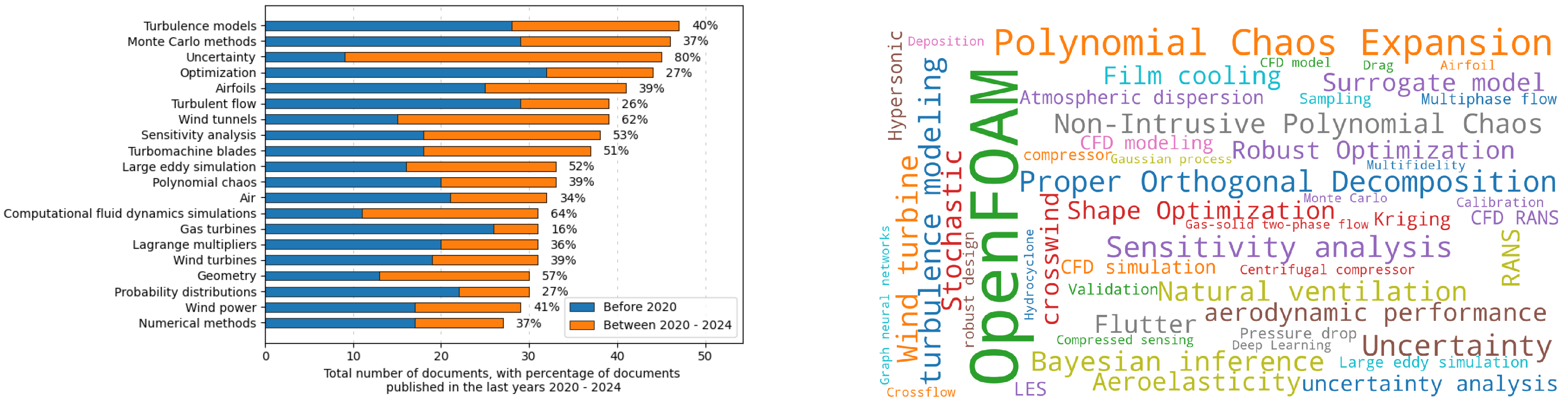
Figure 2.
Temporal evolution of the contribution of different countries to the field of UQ in CFD.
Disclaimer/Publisher’s Note: The statements, opinions and data contained in all publications are solely those of the individual author(s) and contributor(s) and not of MDPI and/or the editor(s). MDPI and/or the editor(s) disclaim responsibility for any injury to people or property resulting from any ideas, methods, instructions or products referred to in the content. |
© 2024 by the authors. Licensee MDPI, Basel, Switzerland. This article is an open access article distributed under the terms and conditions of the Creative Commons Attribution (CC BY) license (http://creativecommons.org/licenses/by/4.0/).
Copyright: This open access article is published under a Creative Commons CC BY 4.0 license, which permit the free download, distribution, and reuse, provided that the author and preprint are cited in any reuse.


