Subdiffusion Equation with Fractional Caputo Time Derivative with Respect to Another Function in Modeling Superdiffusion

1. Introduction

Diffusion processes are generated by a random walk of molecules. In the standard continuous time random walk (CTRW) model [1,2,3,4,5,6,7], this process is characterized by two probability densities $\psi \left(\Delta t\right)$ and $\lambda \left(\Delta x\right)$ describing jumps of a single particle, $\Delta t$ is the waiting time for the particle to jump, $\Delta x$ is the length of the jump. In normal diffusion, both distributions have finite moments. In the case of anomalous diffusion at least one of these distributions has a heavy tail, which causes it to have infinite moments. In the case of subdiffusion the waiting time for the molecule to jump is anomalously long, $\psi$ has a heavy tail. Subdiffusion can occur in media in which the movement of molecules is very hindered, such as gels or porous media. When jumps of molecules can be anomalously long, which occurs in turbulent media, we are dealing with superdiffusion. In this case, $\lambda$ has a heavy tail, the second central moment of this distribution is infinite. Within the CTRW model, anomalous diffusion is described by an equation with a fractional derivative, in the subdiffusion equation it is a fractional derivative with respect to time, and in the superdiffusion equation it is a fractional derivative with respect to the spatial variable [1,2,3,6,7,8,9,10,11,12,13,14,15].

Types of diffusion processes are often defined by the temporal evolution of the mean square displacement (MSD) ${\sigma }^2$ of a diffusing molecule [1,16,17,18,19],

$$\begin{array}{c}\hfill {\sigma }^2\left(t\right)\sim \left\{\begin{array}{c}{t}^{2/\gamma },2>\gamma >1,\mathrm{for}\mathrm{superdiffusion},\\ t,\mathrm{for}\mathrm{normal}\mathrm{diffusion},\\ t^{\alpha },0<\alpha <1,\mathrm{for}\mathrm{ordinary}\mathrm{subdiffusion}.\end{array}\right.\end{array}$$

(1)

In an unbounded homogeneous one-dimensional system, there is ${\sigma }^2\left(t\right)=2D_{\alpha }{t}^{\alpha }/\mathsf{\Gamma }(1+\alpha )$ with $0<\alpha <1$ for subdiffusion and ${\sigma }^2\left(t\right)=2D_{\alpha =1}t$ for normal diffusion, $D_{\alpha }$ is a subdiffusion coefficient given in the units of ${\mathrm{m}}^2/\sec$ (or normal diffusion coefficient when $\alpha =1$). However, for superdiffusion described by a fractional differential equation, the relation takes the form

$${\sigma }^2\left(t\right)=\kappa t^{2/\gamma }$$

(2)

with $\kappa =\infty$. Thus, for fractional superdiffusion ${\sigma }^2\left(t\right)=\infty$ holds which is a rather useless relation because it does not define the parameter $\gamma$.

Another disadvantage of the fractional superdiffusion model is the difficulty in assigning boundary conditions at a partially permeable membrane. The reason for this is that the fractional derivative with respect to the spatial variable has a non-local character. Then, non-local boundary conditions have been used. This causes difficulties in using the fractional superdiffusion equation to model the process in membrane systems.

We propose a model of superdiffusion that leads to Eq. (2) with $\kappa <\infty$, and in which local boundary conditions at a membrane, such as those for subdiffusion or normal diffusion, can be applied. The model is based on the g–subdiffusion equation with fractional Caputo time derivative with respect to another function, see Refs. [20,21]. The g–subdiffusion equation can be interpreted as the ordinary subdiffusion equation with a changed time scale controlled by the function g. The change in time scale is generated by a deterministic process. We add that a change in time scale can also be generated by a stochastic process in the subordinate method [6,22,23,24,25,26]. So far, the g–subdiffusion equation has been used to describe a smooth transition from subdiffusion to ultraslow diffusion (slow subdiffusion) [20], to superdiffusion [27], to subdiffusion with a changed parameter $\alpha$ [28], to model the transition between different types of anomalous diffusion with irreversible reactions [29], and to describe anomalous diffusion of drugs released from densely packed gel beads immersed in water [30]. In this paper, this equation is used to describe superdiffusion in the entire time domain. We consider diffusion in a one-dimensional unbounded system, except in Sec. V, where the filtration process in a membrane system is modeled.

2. Anomalous Diffusion Equations

In this section we show the ordinary subdiffusion and fractional superdiffusion equations, along with their Green’s functions. The Green’s function (GF) $P(x,t|x_0)$ is defined as the solution to the equation with the initial condition $P(x,0|x_0)=\delta (x-x_0)$, $\delta$ is the delta–Dirac function, and - in an unbounded system - with boundary conditions $P(\pm \infty ,t|x_0)=0$. The GF is interpreted as the probability density of finding a molecule at point x at time t, $x_0$ being the initial position of the molecule at time $t=0$.

2.1. Ordinary Subdiffusion Equation

The ordinary subdiffusion equation reads

$${\displaystyle \frac{{‌}^C{\partial }^{\alpha }{P}_{\alpha }(x,t|x_0)}{\partial t^{\alpha }}}=D_{\alpha }{\displaystyle \frac{{\partial }^2{P}_{\alpha }(x,t|x_0)}{\partial x^2}},$$

(3)

where $0<\alpha <1$,

$${\displaystyle \frac{{‌}^C{d}^{\alpha }f\left(t\right)}{d{t}^{\alpha }}}={\displaystyle \frac{1}{\mathsf{\Gamma }(1-\alpha )}}{\int }_0^t{(t-u)}^{-\alpha }{f}^{\prime }\left(u\right)du$$

(4)

is the fractional Caputo time derivative, $f^{\prime }\left(u\right)=df\left(u\right)/du$.

The Green’s function for Eq. (3) is (see, among others, Refs. [31,32,33,34,35])

$$\begin{array}{c}\hfill P_{\alpha }(x,t|x_0)={\displaystyle \frac{1}{2\sqrt{D_{\alpha }}}}{f}_{-1+\alpha /2,\alpha /2}\left(t;{\displaystyle \frac{|x-x_0|}{\sqrt{D_{\alpha }}}}\right)={\displaystyle \frac{1}{2\sqrt{D_{\alpha }{t}^{\alpha }}}}\sum _{j=0}^{\infty }{\displaystyle \frac{1}{j!\mathsf{\Gamma }(1-\alpha (j+1)/2)}}{\left(-{\displaystyle \frac{|x-x_0|}{\sqrt{D_{\alpha }{t}^{\alpha }}}}\right)}^j.\end{array}$$

(5)

Formally, the Green’s function for normal diffusion can be obtained from the Green’s function for ordinary subdiffusion Eq. (5) in the limit $\alpha \to 1^{-}$; in the following this limit is also noted as $\alpha =1$.

$$P_{\alpha =1}(x,t|x_0)={\displaystyle \frac{1}{2\sqrt{\pi Dt}}}{\mathrm{e}}^{-{\displaystyle \frac{{(x-x_0)}^2}{4Dt}}}.$$

(6)

The above function fulfils the normal diffusion equation

$${\displaystyle \frac{\partial P_{\alpha =1}(x,t|x_0)}{\partial t}}=D{\displaystyle \frac{{\partial }^2{P}_{\alpha =1}(x,t|x_0)}{\partial x^2}}.$$

(7)

In terms of the ordinary Laplace transform

$$\mathcal{L}\left[f\left(t\right)\right]\left(s\right)={\int }_0^{\infty }{\mathrm{e}}^{-st}f\left(t\right)dt,$$

(8)

due to the following relation

$$\mathcal{L}\left[{\displaystyle \frac{{‌}^C{d}^{\alpha }f\left(t\right)}{d{t}^{\alpha }}}\right]\left(s\right)=s^{\alpha }\mathcal{L}\left[f\left(t\right)\right]\left(s\right)-s^{\alpha -1}f\left(0\right),\alpha \in (0,1),$$

(9)

the ordinary subdiffusion equation is

$$s^{\alpha }\mathcal{L}\left[P_{\alpha }(x,t|x_0)\right]\left(s\right)-s^{\alpha -1}{P}_{\alpha }(x,0|x_0)=D_{\alpha }{\displaystyle \frac{{\partial }^2\mathcal{L}\left[P_{\alpha }(x,t|x_0)\right]\left(s\right)}{\partial x^2}}.$$

(10)

The solution to Eq. (10) is the Laplace transform of Green’s function,

$$\mathcal{L}\left[P_{\alpha }(x,t|x_0)\right]\left(s\right)={\displaystyle \frac{1}{2\sqrt{D_{\alpha }}{s}^{1-\alpha /2}}}{\mathrm{e}}^{-|x-x_0|{\displaystyle \frac{s^{\alpha /2}}{\sqrt{D_{\alpha }}}}}.$$

(11)

2.2. Factional Superdiffusion Equation

The fractional superdiffusion equation reads

$${\displaystyle \frac{\partial P_{\gamma }(x,t|x_0)}{\partial t}}=D_{\gamma }{\displaystyle \frac{{\partial }^{\gamma }{P}_{\gamma }(x,t|x_0)}{{\partial \left|x\right|}^{\gamma }}},$$

(12)

where the Riesz–type fractional derivative is defined by its Fourier transform, $\mathcal{F}\left(k\right)={\int }_{-\infty }^{\infty }{\mathrm{e}}^{ikx}f\left(x\right)dx$, as

$$\mathcal{F}\left[{\displaystyle \frac{d^{\gamma }f\left(x\right)}{{d\left|x\right|}^{\gamma }}}\right]\left(k\right)=-{\left|k\right|}^{\gamma }\mathcal{F}\left(k\right).$$

(13)

The Green’s function for Eq. (12) is, see Ref. [27] and the references cited therein,

$$\begin{array}{c}\hfill P_{\gamma }(x,t|x_0)={\displaystyle \frac{1}{\sqrt{\pi }|x-x_0|}}{H}_{12}^{11}\left({\displaystyle \frac{|x-x_0{|}^{\gamma }}{2^{\gamma }{D}_{\gamma }t}}\left|\begin{array}{c}(1,1)\\ (1/2,\gamma /2)(1,\gamma /2)\end{array}\right.\right)\\ \hfill ={\displaystyle \frac{1}{\gamma \sqrt{\pi }{\left(D_{\gamma }t\right)}^{1/\gamma }}}\sum _{j=0}^{\infty }{\displaystyle \frac{\mathsf{\Gamma }(1/\gamma +2j/\gamma )}{j!\mathsf{\Gamma }(1/2+j)}}{\left(-{\displaystyle \frac{{(x-x_0)}^2}{4{\left(D_{\gamma }t\right)}^{2/\gamma }}}\right)}^j,\end{array}$$

(14)

where H denotes the H–Fox function [36].

3. $\mathit{G}$–Subdiffusion Equation

The g–subdiffusion equation is a modified ordinary subdiffusion equation Eq. (3). The modification consists in changing the time variable t to a function $g\left(t\right)$,

$$t\to g\left(t\right),$$

(15)

$g\left(t\right)$ is given in a time unit and meets the conditions

$$g\left(0\right)=0,g(\infty )=\infty ,g^{\prime }\left(t\right)>0.$$

(16)

In order to determine the equation and Green’s function for the g–subdiffusion process, the Laplace transform with respect to the function g, which is called the g–Laplace transform, can be used [37,38]

$${\mathcal{L}}_g\left[f\left(t\right)\right]\left(s\right)={\int }_0^{\infty }{\mathrm{e}}^{-sg\left(t\right)}f\left(t\right)g^{\prime }\left(t\right)dt.$$

(17)

The relation between the Laplace transforms is as follows

$${\mathcal{L}}_g\left[f\left(t\right)\right]\left(s\right)=\mathcal{L}\left[f\left(g^{-1}\left(t\right)\right)\right]\left(s\right).$$

(18)

Eq. (18) provides the relation

$${\mathcal{L}}_g\left[f\left(t\right)\right]\left(s\right)=\mathcal{L}\left[h\left(t\right)\right]\left(s\right)\iff f\left(t\right)=h\left(g\left(t\right)\right).$$

(19)

Knowing the ordinary Laplace transform, the above equation is helpful in determining the inverse g–Laplace transform. The examples are

$${\mathcal{L}}_g^{-1}\left[{\displaystyle \frac{1}{s^{\mu +1}}}\right]\left(t\right)={\displaystyle \frac{g^{\mu }\left(t\right)}{\mathsf{\Gamma }(1+\mu )}},\mu >-1,$$

(20)

$$\begin{array}{c}\hfill {\mathcal{L}}_g^{-1}\left[s^{\nu }{\mathrm{e}}^{-a{s}^{\beta }}\right]\left(t\right)\equiv f_{\nu ,\beta }(g\left(t\right);a)={\displaystyle \frac{1}{g^{1+\nu }\left(t\right)}}\sum _{j=0}^{\infty }{\displaystyle \frac{1}{j!\mathsf{\Gamma }(-\nu -\beta j)}}{\left(-{\displaystyle \frac{a}{g^{\beta }\left(t\right)}}\right)}^j,\end{array}$$

(21)

$a,\beta >0$.

The conclusion from Eqs. (19) is that the change in the time variable can be made according to the relation

$$t\to g\left(t\right)\iff \mathcal{L}\left[P_{\alpha }(x,t|x_0)\right]\left(s\right)\to {\mathcal{L}}_g\left[P_g(x,t|x_0)\right]\left(s\right).$$

(22)

Applying the rule Eq. (22) to Eq. (10), we get

$$s^{\alpha }{\mathcal{L}}_g\left[P_{g,\alpha }(x,t|x_0)\right]\left(s\right)-s^{\alpha -1}{P}_{g,\alpha }(x,0|x_0)=D_{\alpha }{\displaystyle \frac{{\partial }^2{\mathcal{L}}_g\left[P_{g,\alpha }(x,t|x_0)\right]\left(s\right)}{\partial x^2}},$$

(23)

where $P_{g,\alpha }(x,0|x_0)=\delta (x-x_0)$. Due to the relation

$${\mathcal{L}}_g\left[{\displaystyle \frac{{‌}^C{d}_g^{\alpha }f\left(t\right)}{d{t}^{\alpha }}}\right]\left(s\right)=s^{\alpha }{\mathcal{L}}_g\left[f\left(t\right)\right]\left(s\right)-s^{\alpha -1}f\left(0\right),\alpha \in (0,1),$$

(24)

where

$${\displaystyle \frac{{‌}^C{d}_g^{\alpha }f\left(t\right)}{d{t}^{\alpha }}}={\displaystyle \frac{1}{\mathsf{\Gamma }(1-\alpha )}}{\int }_0^t{[g\left(t\right)-g\left(u\right)]}^{-\alpha }{f}^{\prime }\left(u\right)du$$

(25)

is the Caputo fractional derivative with respect to another function g[21,37,38], the inverse g–Laplace transform of Eq. (24) reads

$${\displaystyle \frac{{‌}^C{\partial }_g^{\alpha }{P}_{g,\alpha }(x,t|x_0)}{\partial t^{\alpha }}}=D_{\alpha }{\displaystyle \frac{{\partial }^2{P}_{g,\alpha }(x,t|x_0)}{\partial x^2}}.$$

(26)

When $\alpha \to 1^{-}$ there is

$${\displaystyle \frac{{‌}^C{d}_{g}f\left(t\right)}{dt}}={\lim }_{\alpha \to 1^{-}}{\displaystyle \frac{{‌}^C{d}_g^{\alpha }f\left(t\right)}{d{t}^{\alpha }}}={\displaystyle \frac{f^{\prime }\left(t\right)}{g^{\prime }\left(t\right)}}.$$

(27)

Combining Eqs. (11) and (22) we get the Green’s function for g-subdiffusion equation in terms of the g-Laplace transform

$${\mathcal{L}}_g\left[P_{g,\alpha }(x,t|x_0)\right]\left(s\right)={\displaystyle \frac{1}{2\sqrt{D_{\alpha }}{s}^{1-\alpha /2}}}{\mathrm{e}}^{-|x-x_0|{\displaystyle \frac{s^{\alpha /2}}{\sqrt{D_{\alpha }}}}}.$$

(28)

Eqs. (21) and (28) provide

$$\begin{array}{c}\hfill P_{g,\alpha }(x,t|x_0)={\displaystyle \frac{1}{2\sqrt{D_{\alpha }}}}{f}_{-1+\alpha /2,\alpha /2}\left(g\left(t\right);{\displaystyle \frac{|x-x_0|}{\sqrt{D_{\alpha }}}}\right)={\displaystyle \frac{1}{2\sqrt{D_{\alpha }{g}^{\alpha }\left(t\right)}}}\sum _{j=0}^{\infty }{\displaystyle \frac{1}{j!\mathsf{\Gamma }(1-\alpha (j+1)/2)}}{\left(-{\displaystyle \frac{|x-x_0|}{\sqrt{D_{\alpha }{g}^{\alpha }\left(t\right)}}}\right)}^j.\end{array}$$

(29)

Since P is translational invariant and symmetric with respect to the point $x_0$, there is

$${\sigma }^2\left(t\right)=2{\int }_0^{\infty }{x}^{2}P(x,t|0)dx.$$

(30)

In terms of the g-Laplace transform we have ${\mathcal{L}}_g\left[{\sigma }^2\left(t\right)\right]\left(s\right)={\int }_0^{\infty }{x}^2\left[P_{g,\alpha }(x,t|0)\right]\left(s\right)dx=2D_{\alpha }/s^{1+\alpha }$. Finally, we obtain for g-subdiffusion

$${\sigma }_g^2\left(t\right)={\displaystyle \frac{2D_{\alpha }}{\mathsf{\Gamma }(1+\alpha )}}{g}^{\alpha }\left(t\right).$$

(31)

4. Using the $\mathit{G}$–Subdiffusion Equation to Describe Superdiffusion

The idea of using the g–subdiffusion equation to describe superdiffusion is based on the definition of the function g which provides Eq. (31) in the form of Eq. (2) with finite $\kappa$.

4.1. Finding the Function g

We assume that a function g provides asymptotic agreement between the Green’s function for g–subdiffusion Eq. (29) and the one for fractional superdiffusion Eq. (14) when $t\to \infty$,

$$P_{g,\alpha }(x,t\to \infty |x_0)=P_{\gamma }(x,t\to \infty |x_0).$$

(32)

Since

$$P_{g,\alpha }(x,t\to \infty |x_0)={\displaystyle \frac{1}{2\sqrt{D_{\alpha }\mathsf{\Gamma }(1-\alpha /2)g^{\alpha }\left(t\right)}}},$$

(33)

$$P_{\gamma }(x,t\to \infty |x_0)={\displaystyle \frac{1}{\gamma \sqrt{\mathsf{\Gamma }(1/\gamma )}{\left(D_{\gamma }t\right)}^{1/\gamma }}},$$

(34)

we get from the above equations

$$\tilde{g}\left(t\right)=E{t}^{{\displaystyle \frac{2}{\gamma \alpha }}},$$

(35)

where

$$E={\left({\displaystyle \frac{\pi \gamma D_{\gamma }^{1/\gamma }}{2\sqrt{D_{\alpha }}\mathsf{\Gamma }(1/\gamma )\mathsf{\Gamma }(1-\alpha /2)}}\right)}^{2/\alpha },$$

(36)

$\tilde{g}$ is the designation of the function g for superdiffusion. We note that $\sqrt{g^{\alpha }\left(t\right)D_{\alpha }}=\pi \gamma D_{\gamma }^{1/\gamma }{t}^{1/\gamma }/\left[2\mathsf{\Gamma }(1/\gamma )\sqrt{\pi }\right]$, which causes the subdiffusion coefficient $D_{\alpha }$ to be eliminated from the Green’s function. Eqs. (29) and (35) provide the Green’s function describing superdiffusion

$$\begin{array}{c}\hfill P_{\tilde{g},\alpha }(x,t|x_0)={\displaystyle \frac{\mathsf{\Gamma }(1/\gamma )\mathsf{\Gamma }(1-\alpha /2)}{\pi \gamma {\left(D_{\gamma }t\right)}^{1/\gamma }}}\sum _{j=0}^{\infty }{\displaystyle \frac{1}{j!\mathsf{\Gamma }(1-\alpha (j+1/2)}}{\left(-{\displaystyle \frac{|x-x_0|2\mathsf{\Gamma }(1/\gamma )\mathsf{\Gamma }(1-\alpha /2)}{\pi \gamma {\left(D_{\gamma }t\right)}^{1/\gamma }}}\right)}^j.\end{array}$$

(37)

The time evolution of MSD is

$${\sigma }^2\left(t\right)={\kappa }_{\tilde{g}}{t}^{{\displaystyle \frac{2}{\gamma }}},$$

(38)

with

$${\kappa }_{\tilde{g}}={\left({\displaystyle \frac{\pi \gamma D_{\gamma }^{1/\gamma }}{\sqrt{2}\mathsf{\Gamma }(1/\gamma )\mathsf{\Gamma }(1-\alpha /2)}}\right)}^2.$$

(39)

4.2. G–Superdiffusion Equation

The g–superdiffusion equation, which is defined as the g–subdiffusion equation describing superdiffusion, reads

$${\displaystyle \frac{{‌}^C{\partial }^{\gamma ,\alpha }P(x,t|x_0)}{\partial t^{\gamma ,\alpha }}}=\tilde{D}{\displaystyle \frac{{\partial }^{2}P(x,t|x_0)}{\partial x^2}},$$

(40)

where

$${\displaystyle \frac{{‌}^C{\partial }^{\gamma ,\alpha }f\left(t\right)}{\partial t^{\gamma ,\alpha }}}={\displaystyle \frac{1}{\mathsf{\Gamma }(1-\alpha )}}{\int }_0^t{\displaystyle \frac{f^{\prime }\left(u\right)}{(t^{\frac{2}{\gamma \alpha }}-u^{\frac{2}{\gamma \alpha }})}}du,$$

(41)

$\tilde{D}$ is the superdiffusion coefficient given in the units of $m^2/{\sec }^{2/\gamma }$. This coefficient is related to other parameters as $\tilde{D}={[\pi \gamma D_{\gamma }^{1/\gamma }/\left(2\mathsf{\Gamma }(1/\gamma )\mathsf{\Gamma }(1-\alpha /2)\right)]}^2$.

4.3. Stochastic Interpretation

The ordinary subdiffusion equation can be derived from the ordinary continuous time random walk (CTRW) model. The g–subdiffusion equation can be derived from a modified CTRW model (called the g-CTRW model), which becomes the ordinary CTRW model when $g\left(t\right)\equiv t$[39]. Let $\Delta t_i$ be the waiting time for the particle to i-th jump. The sequences of waiting times for the particle to jump for both processes are related to each other as follows

$${\mathcal{P}}_n[\underset{ordinarysubdif.}{\underbrace{(\Delta t_1,\Delta t_2,\dots ,\Delta t_n)}}]={\mathcal{P}}_n[\underset{gsubdif.}{\underbrace{(g^{-1}\left(\Delta t_1\right),g^{-1}\left(\Delta t_2\right),\dots ,g^{-1}\left(\Delta t_n\right))}}],$$

(42)

where $P_n$ is the probability distribution of the sequence of n waiting times for a particle to jump. The average number of a particle jumps for g–subdiffusion is given by the formula [27]

$$〈n\left(t\right)〉={\displaystyle \frac{g^{\alpha }\left(t\right)}{\tau \mathsf{\Gamma }(1+\alpha )}},$$

(43)

where $\tau$ is a parameter given in the unit of ${\sec }^{\alpha }$. The mean jumps frequency is defined as $f\left(t\right)=d〈n\left(t\right)〉/dt$, for g–subdiffusion there is

$$f\left(t\right)={\displaystyle \frac{g^{\prime }\left(t\right)}{\tau \mathsf{\Gamma }\left(\alpha \right)g^{1-\alpha }\left(t\right)}}.$$

(44)

From Eqs. (35) and (44) we get

$$f\left(t\right)=\tilde{E}{t}^{{\displaystyle \frac{2}{\gamma }}-1}.$$

(45)

where $\tilde{E}=2E^{\alpha }/\left(\gamma \tau \mathsf{\Gamma }(1+\alpha )\right)$. Eq. (45) shows that the superdiffusion effect in the g–subdiffusion process is caused by an increasing frequency of particle jumps. This is a different superdiffusion interpretation than its interpretation within the ordinary CTRW model. In the latter model the superdiffusion effect originates from anomalously long particle jumps performed with relatively high probabilities whereas jump frequency is constant.

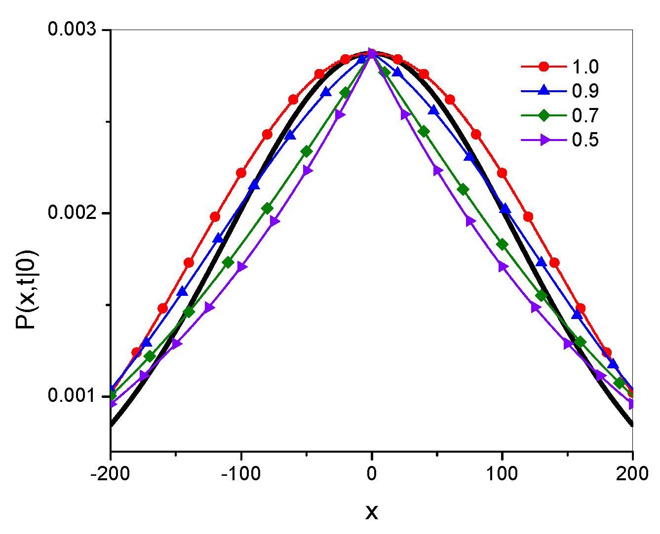
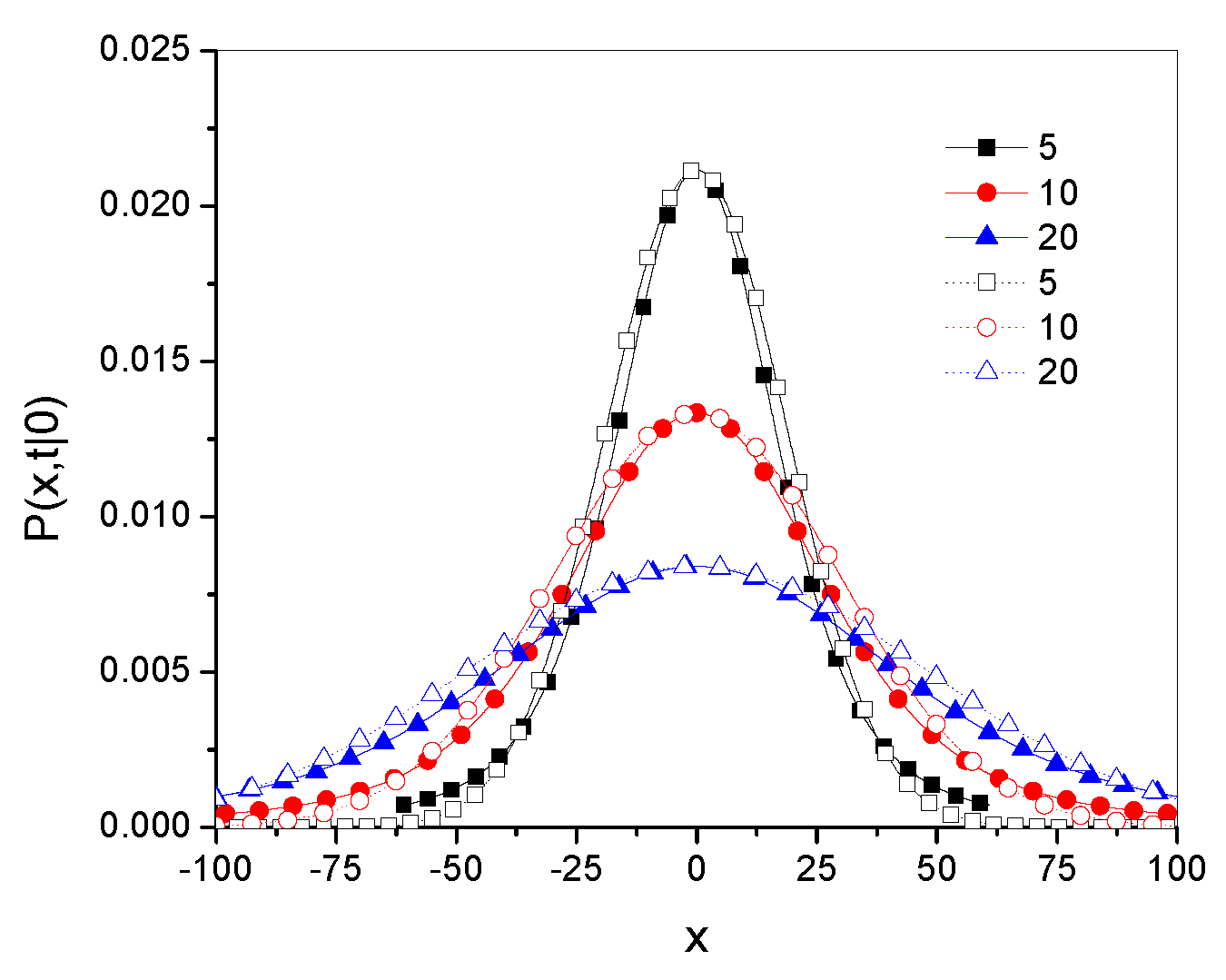
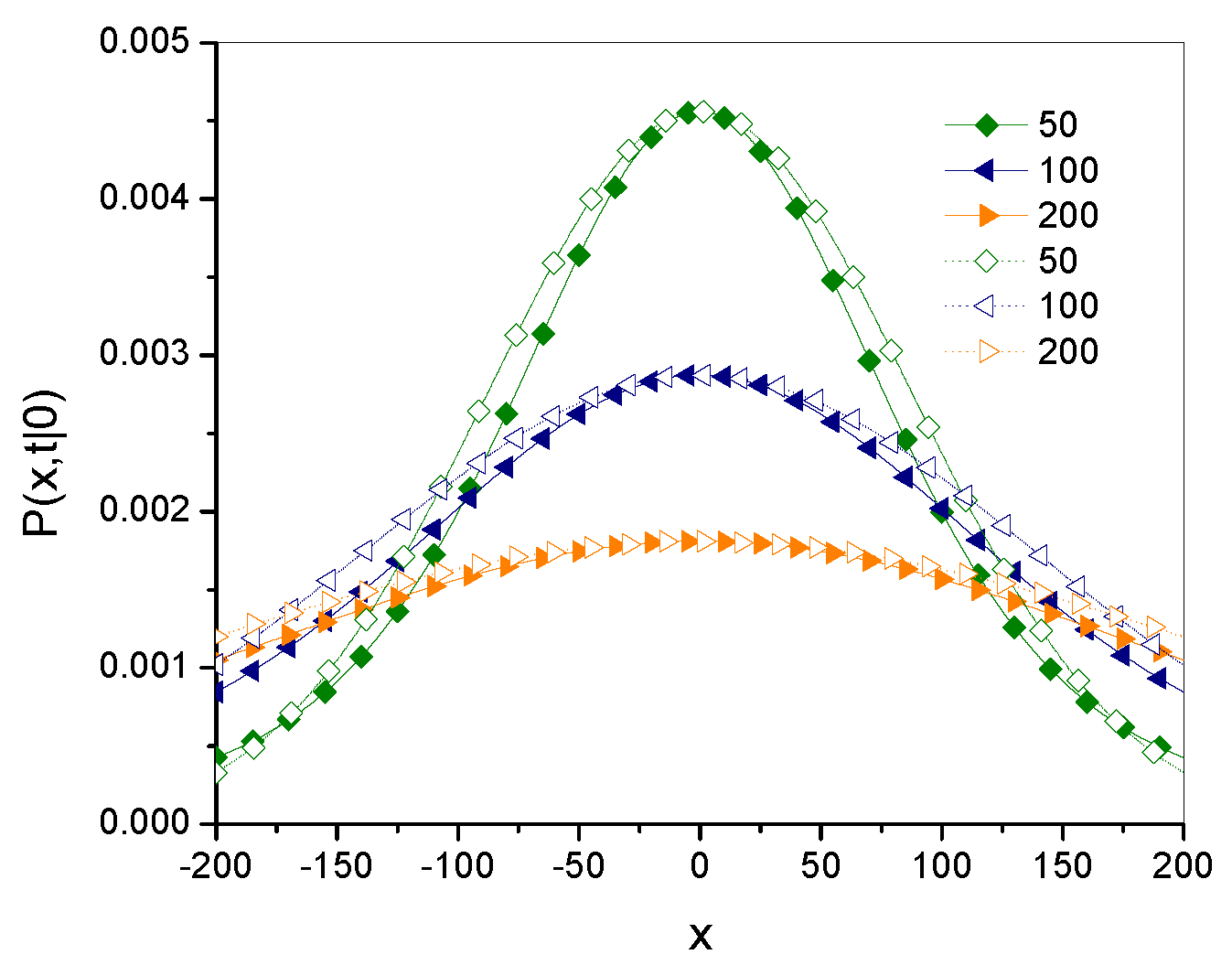
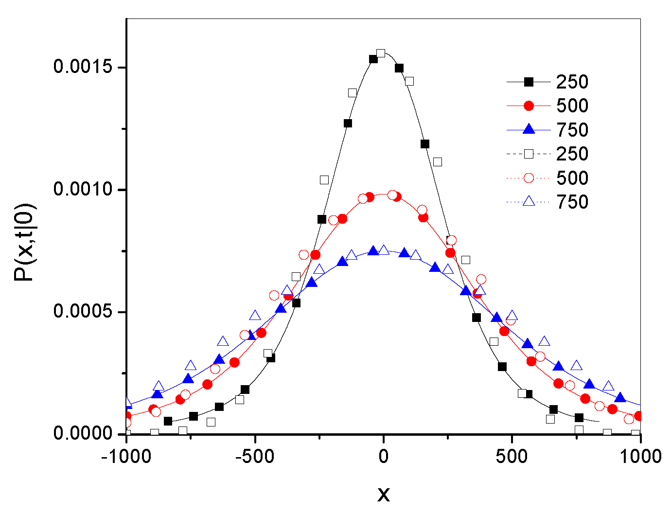
4.4. The Influence of Parameter $\alpha$ on g–Superdiffusion

Example plots of the Green’s functions $P_{\gamma }$ and $P_{\tilde{g},\alpha }$ are shown in Figure 1; the Green’s functions have been plotted for 20 leading terms in the series defining the function. Throughout this paper, the values of all parameters and variables are given in arbitrarily chosen units. The qualitative differences between the functions are most visible at point $x=0$. The function $P_{\gamma }$ is smooth, as is the function $P_{\tilde{g},\alpha }$ for $\alpha \to 1^{-}$, while the latter functions for $\alpha <1$ has characteristic spikes at this point.

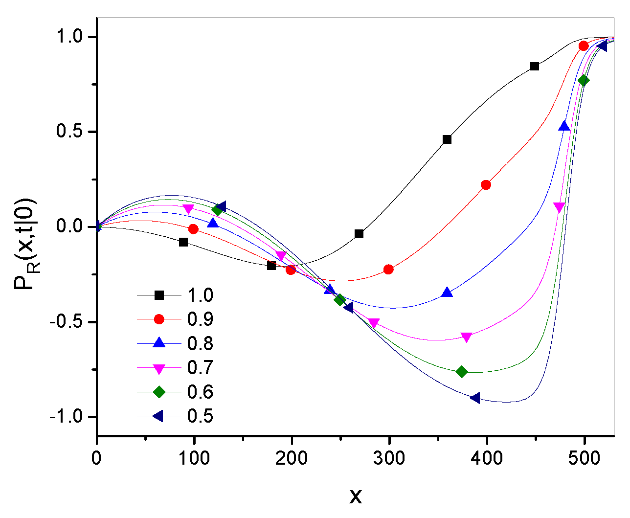
We note that the exponent of the function Eq. (38) is the same as for fractional superdiffusion and depends on the superdiffusion parameter $\gamma$ only, the function ${\kappa }_{\tilde{g}}$ is finite and depends on both parameters $\gamma$ and $\alpha$. In order to check the influence of the parameter $\alpha$ on the Green’s function, we use the relative function $P_R$ showing the relative difference of the Green’s functions $P_{\tilde{g},\alpha }$ and $P_{\gamma }$,

$$P_R(x,t|x_0)={\displaystyle \frac{P_{\gamma }(x,t|x_0)-P_{\tilde{g},\alpha }(x,t|x_0)}{P_{\gamma }(x,t|x_0)}}.$$

(46)

An example of the influence of the parameter $\alpha$ on the Green’s function is shown in Figure 2. The figure suggests that for x not too far from the initial particle position, the functions $P_{\gamma }$ and $P_{\tilde{g},\alpha }$ differ from each other rather little, $P_{\gamma }$ is closer to $P_{\tilde{g},\alpha }$ for larger $\alpha$. For large x, $P_{\gamma }$ dominates over $P_{\tilde{g},\alpha }$. Next we consider the detailed case of $\alpha \to 1^{-}$.

4.5. G-Subdiffusion for $\alpha \to 1^{-}$

Let us write the function $P_{\gamma }$ Eq. (14) in the following form

$$P_{\gamma }(x,t|x_0)={\displaystyle \frac{1}{\gamma \sqrt{\pi }{\left(D_{\gamma }t\right)}^{1/\gamma }}}\sum _{j=0}^{\infty }{\displaystyle \frac{A_j}{j!}}{\left(-{\displaystyle \frac{{(x-x_0)}^2}{4{\left(D_{\gamma }t\right)}^{2/\gamma }}}\right)}^j,$$

(47)

where $A_j=\mathsf{\Gamma }(1/\gamma +2j/\gamma )/[j!\mathsf{\Gamma }(1/2+j)]$. In the limit $\alpha \to 1^{-}$, $P_{\tilde{g},\alpha }$ has a structure similar to $P_{\gamma }$,

$$P_{\tilde{g},\alpha \to 1^{-}}(x,t|x_0)={\displaystyle \frac{1}{\gamma \sqrt{\pi }{\left(D_{\gamma }t\right)}^{1/\gamma }}}\sum _{j=0}^{\infty }{\displaystyle \frac{B_j}{j!}}{\left(-{\displaystyle \frac{{(x-x_0)}^2}{\gamma {\left(D_{\gamma }t\right)}^{2/\gamma }}}\right)}^j,$$

(48)

where $B_j=(\mathsf{\Gamma }(1/\gamma )/\sqrt{\pi }){(2\mathsf{\Gamma }(1/\gamma )/\sqrt{\pi }\gamma )}^j$.

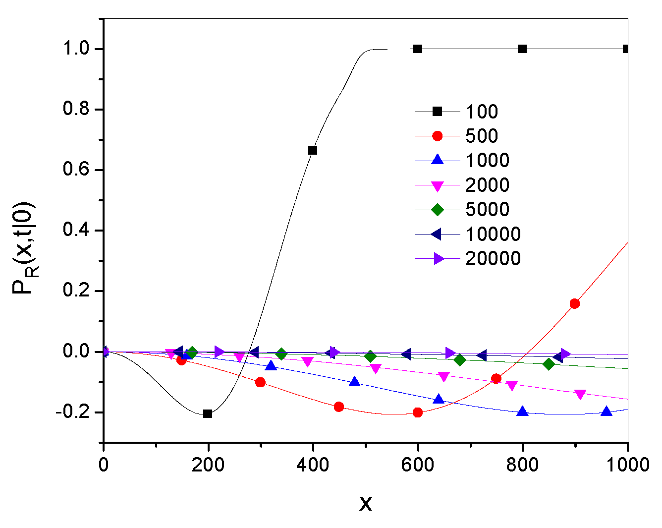
The plots of the relative function

$$P_R(x,t|x_0)={\displaystyle \frac{P_{\gamma }(x,t|x_0)-P_{\tilde{g},\alpha \to 1^{-}}(x,t|x_0)}{P_{\gamma }(x,t|x_0)}}.$$

(49)

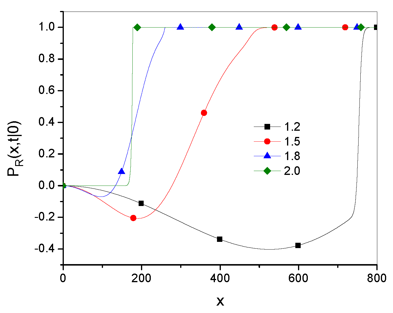
are shown in Figures (Figure 3) and (Figure 4), here $D_{\gamma }=10$, and $x_0=0$. Figure 3 shows that the range of x in which both Green’s functions are close to each other grows with time. Figure 4 shows that for larger values of the parameter $\gamma$ (which corresponds to a smaller superdiffusion effect) the relation $P_{\gamma }\gg P_{\tilde{g},\alpha \to 1^{-}}$ holds in a larger range of x.

Plots of the Green’s functions $P_{\gamma }$ and $P_{\tilde{g},\alpha }$ for different times are shown in Figure 5, Figure 6 and Figure 7 for $\gamma =1.5$, $D_{\gamma }=10$, and $x_0=0$. The plots suggest that both functions are rather close to each other for both short and long times, their qualitative features are also similar.

5. Filtration in a Superdiffusion System

As mentioned, using fractional superdiffusion equations one cannot uniquely define local boundary conditions at a thin membrane, excluding boundary conditions at fully absorbing or fully reflecting walls [40]. The boundary conditions used for this equation are usually non-local, which - in our opinion - causes difficulties in their physical interpretation. However, for the g–superdiffusion equation local boundary conditions can be used because the equation contains an integer-order spatial derivative; these conditions are in practice the same as boundary conditions for ordinary subdiffusion or normal diffusion equations.

The membrane can be used to filter a diffusing substance. Assuming the system is homogeneous in the plane parallel to the membrane, the problem is one-dimensional. Let a thin membrane, placed at point $x=0$, separates vessels A and B. We assume that initially a diffusing molecule is in the vessel A, $x_0<0$. The filtering membrane allows (almost) free movement of molecules from A to B, while molecules trying to pass through the membrane in the opposite direction can be retained at the membrane with probability $\sigma$. Let us assume that the walls bounded the vessels are located at a large distance from the membrane and do not effectively affect the diffusion of molecules through the membrane. Then, the vessels are represented as infinite intervals, $A=(-\infty ,0)$ and $B=(0,\infty )$.

The boundary conditions at the membrane are [41]

$$J_{A,\tilde{g},\alpha }(0^{-},t|x_0)=J_{B,\tilde{g},\alpha }(0^{+},t|x_0),$$

(50)

and

$$P_{A,\tilde{g},\alpha }(0^{-},t|x_0)=\sigma P_{B,\tilde{g},\alpha }(0^{+},t|x_0),$$

(51)

where the g–superdiffusion flux $J_{\tilde{g},\alpha }$ is defined as

$$J_{\tilde{g},\alpha }(x,s|x_0)=-D_{\alpha }{\displaystyle \frac{{‌}^C{\partial }_{\tilde{g}}^{\alpha }}{\partial t^{\alpha }}}{\displaystyle \frac{\partial P_{\tilde{g},\alpha }(x,t|x_0)}{\partial x}}.$$

(52)

The above boundary conditions generate the following Green’s functions (see Ref. [41])

$$P_{A,\tilde{g},\alpha }(x,t|x_0)=P_{\tilde{g},\alpha }(x,t|x_0)+(1-\mathsf{\Lambda })P_{\tilde{g},\alpha }(x,t|2x_M-x_0),$$

(53)

$$P_{B,\tilde{g},\alpha }(x,t|x_0)=\mathsf{\Lambda }{P}_{\tilde{g},\alpha }(x,t|x_0),$$

(54)

where $\mathsf{\Lambda }=2\sigma /(1+\sigma )$.

As example, we consider a filtration process taking place in a subdiffusive medium, such as a turbulent one, in which at the initial moment a homogeneous solution of concentration $C_0$ is in region A and there is no diffusing substance in region B. The initial conditions are $C_A(x,0)=C_0$ and $C_B(x,0)=0$. We are interested in the temporal evolution of the amount of substance in region B. The concentration $C_B(x,t)$ can be calculated using the formula

$$C_{B,\tilde{g},\alpha }(x,t)=C_0{\int }_{-\infty }^0{P}_{B,\tilde{g},\alpha }(x,t|x_0)d{x}_0.$$

(55)

Eq. (55) provide

$$C_{B,\tilde{g},\alpha }(x,t)={\displaystyle \frac{\mathsf{\Lambda }{C}_0}{2}}{f}_{-1,\alpha /2}\left(E{t}^{{\displaystyle \frac{2}{\gamma \alpha }}},{\displaystyle \frac{x}{\sqrt{D}}}\right).$$

(56)

The time evolution of total amount of substance in region B, $W_{B,\tilde{g},\alpha }\left(t\right)={\int }_0^{\infty }{C}_{B,\tilde{g},\alpha }(x,t)dx$, is

$$W_{B,\tilde{g},\alpha }\left(t\right)={\displaystyle \frac{\mathsf{\Lambda }{C}_0{E}^{\alpha /2}}{\mathsf{\Gamma }(1+\alpha /2)}}{t}^{{\displaystyle \frac{1}{\gamma }}}.$$

(57)

Eqs. (56) and (57) can be easily derived when we use the g–Laplace transform of the above equations and Eqs (20), (21), (28), and (35). We add that for ordinary subdiffusion with parameter $\alpha$ the rate of the filtration process is $W_{B,\alpha }\left(t\right)\sim t^{\alpha /2}$[41]. Comparing this equation with Eq. (57) we obtain a relation showing the difference in filtration for the processes, $W_{B,\tilde{g},\alpha }\left(t\right)\sim t^{\eta }{W}_{B,\alpha }\left(t\right)$ with $\eta =(1/\gamma )-(\alpha /2)>0$.

6. Final Remarks

The g–subdiffusion equation with the fractional Caputo derivative with respect to another function can be interpreted as the ordinary subdiffusion equation with a changed time variable. So far, the g–subdiffusion equation has been mainly used to describe a smooth transition from subdiffusion to another type of diffusion [20,27] or subdiffusion with a changed parameter $\alpha$ [28]. In this paper, this equation is used to describe superdiffusion in the entire time domain. The characteristic features of the g–superdiffusion equation are as follows.

• The g–superdiffusion equation is defined as the g–subdiffusion equation Eq. (26) with the function g given by Eq. (35). This equation can be written in the equivalent form Eq. (40), which contains a Caputo-type fractional time derivative controlled by two parameters $\gamma \in (1,2)$ and $\alpha \in (0,1)$. The parameter $\gamma$ is the exponent of the time evolution of MSD Eq. (38), which defines the type of diffusion. This parameter also defines the order of the Riesz-type derivative with respect to the spatial variable in the fractional superdiffusion equation which gives the same Green’s function as the g–subdiffusion equation in the limit $t\to \infty$. Thus, it can be said that these equations give an equivalent description of the process in the long-time limit. The parameter $\alpha$ controls the rate of convergence of the Green’s functions.
• More general, solutions of the g–subdiffusion equation goes asymptotically to solutions of the fractional superdiffusion equation when the initial and boundary conditions, and the parameter $\gamma$ are the same for both equations.
• It appears that the parameter $\alpha$ for which the Green’s functions for g–superdiffusion are qualitatively most similar to the one for fractional superdiffusion is $\alpha =1$. This case is considered in Sec. 4.E.
• The g–subdiffusion equation is "local in space", so "typical" boundary conditions at partially permeable walls can be involved in the superdiffusion model.
• The stochastic interpretation of g–superdiffusion process is that the jump frequency of a diffusing particle increases over time to infinity. The probability distribution of the jump lengths of a diffusing molecule has finite moments.
• The Green’s function for g–subdiffusion provides ${\sigma }^2\left(t\right)=\kappa t^{2/\gamma }$ with $\kappa <\infty$.

An effective method for solving the g–superdiffusion equations is the method of Laplace transform with respect to the function $\tilde{g}$ Eq. (35).

References

- R. Metzler and J. Klafter, The random walk’s guide to anomalous diffusion: a fractional dynamics approach, Phys. Rep. 339, 1 (2000). [CrossRef]
- R. Metzler, J. Klafter, and I. M. Sokolov, Anomalous transport in external fields: Continuous time random walks and fractional diffusion equations extended, Phys. Rev. E 58, 1621 (1998). [CrossRef]
- A. Compte, Stochastic foundations of fractional dynamics, Phys. Rev. E 53, 4191 (1996). [CrossRef]
- S.I. Denisov and H. Kantz, Continuous-time random walk with a superheavy-tailed distribution of waiting times, Phys. Rev. E 83, 041132 (2011). [CrossRef]
- E. W. Montroll and G. H. Weiss, Random walks on lattices. II, J. Math. Phys. 6, 167 (1965).
- J. Klafter and I. M. Sokolov, First Step in Random Walks. From Tools to Applications (Oxford UP, New York, 2011).
- E. Barkai, R. Metzler, and J. Klafter, From continuous time random walks to the fractional Fokker-Planck equation, Phys. Rev. E 61, 132 (2000). [CrossRef]
- E. Barkai, Fractional Fokker-Planck equation, solution, and application, Phys. Rev. E 63, 046118 (2001).
- R. Klages, G. Radons, and I. M. Sokolov, Anomalous Transport: Foundations and Applications (Wiley, New York, 2008).
- I. M. Sokolov, J. Klafter, and A. Blumen, Fractional kinetics, Phys. Today 55, 11, 48-54 (2002).
- I. M. Sokolov and J. Klafter, From diffusion to anomalous diffusion: a century after Einstein’s Brownian motion, Chaos 15, 026103 (2005). [CrossRef]
- R. Hilfer and L. Anton, Fractional master equations and fractal time random walks, Phys. Rev. E 51, R848 (1995). [CrossRef]
- W. Wyss, The fractional diffusion equation, J. Math. Phys. 27, 2782 (1986).
- A. V. Chechkin, J. Klafter, and I. M. Sokolov, Fractional Fokker-Planck equation for ultraslow kinetics, Europhys. Lett. 63, 326 (2003). [CrossRef]
- A. V. Chechkin, V. Y. Gonchar, R. Gorenflo, N. Korabel, and I. M. Sokolov, Generalized fractional diffusion equations for accelerating subdiffusion and truncated Levy flights, Phys Rev. E 78, 021111 (2008). [CrossRef]
- E. Barkai, Y. Garini, and R. Metlzer, Strange kinetics of single molecules in living cells, Phys. Today 65, 29 (2012). [CrossRef]
- R. Metzler, J. H. Jeon, A. G. Cherstvy, and E. Barkai, Anomalous diffusion models and their properties: non-stationarity, non-ergodicity, and ageing at the centenary of single particle tracking, Phys. Chem. Chem. Phys. 16, 24128 (2014). [CrossRef]
- A. G. Cherstvy, H. Safdari, and R. Metzler, Anomalous diffusion, nonergodicity, and ageing for exponentially and logarithmically time–dependent diffusivity: striking differences for massive versus massless particles, J. Phys. D: Appl. Phys. 54, 195401 (2021).
- R. Metzler and J. Klafter, The restaurant at the end of the random walk: recent developments in the description of anomalous transport by fractional dynamics, J. Phys. A 37, R161 (2004). [CrossRef]
- T. Kosztołowicz and A. Dutkiewicz, Subdiffusion equation with Caputo fractional derivative with respect to another function, Phys. Rev. E 104, 014118 (2021). [CrossRef]
- R. Almeida, A Caputo fractional derivative of a function with respect to another function, Commun. Nonlinear Sci. Numer. Simul. 44, 460 (2017). [CrossRef]
- I. M. Sokolov, Thermodynamics and fractional Fokker-Planck equations, Phys. Rev. E 63, 056111 (2001). [CrossRef]
- W. Feller, An introduction to probability theory and its applications, Vol. 2 (Wiley, New York, 1968).
- A. V. Chechkin, F. Seno, R. Metzler, and I. M. Sokolov, Brownian yet non-Gaussian diffusion: From superstatistics to subordination of diffusing diffusivities, Phys. Rev. X 7, 021002 (2017). [CrossRef]
- B. Dybiec and E. Gudowska–Nowak, Subordinated diffusion and continuous time random walk asymptotics, Chaos 20, 043129 (2010). [CrossRef]
- A. Chechkin and I. M. Sokolov, Relation between generalized diffusion equations and subordination schemes, Phys. Rev. E 103, 032133 (2021). [CrossRef]
- T. Kosztołowicz, Subdiffusion equation with fractional Caputo time derivative with respect to another function in modeling transition from ordinary subdiffusion to superdiffusion, Phys. Rev. E 107, 064103 (2023). [CrossRef]
- T. Kosztołowicz and A. Dutkiewicz, Composite subdiffusion equation that describes transient subdiffusion, Phys. Rev. E 106, 044119 (2022). [CrossRef]
- T. Kosztołowicz, First passage time for the g-subdiffusion process of vanishing particles, Phys. Rev. E 106, L022104 (2022).
- T. Kosztołowicz, A. Dutkiewicz, K. D. Lewandowska, S. Wa̧sik, and M. Arabski, Subdiffusion equation with Caputo fractional derivative with respect to another function in modeling diffusion in a complex system consisting of matrix and channels, Phys. Rev. E 106, 044138 (2022).
- T. Kosztołowicz, From the solutions of diffusion equation to the solutions of subdiffusive one, J. Phys. A: Math. Gen. 37, 10779 (2004).
- F. Mainardi, The fundamental solutions for the fractional diffusion–wave equation, Appl. Math. Lett. 9, 23 (1996). [CrossRef]
- F. Mainardi, Y. Luchko, and G. Pagnini, The fundamental solutions of the space–time fractional diffusion equation, Fract. Calculus Appl. Anal. 4, 153 (2001).
- F. Mainardi, G. Pagnini, and R. K. Saxena, Fox H functions in fractional diffusion, J. Comput. Appl. Math. 178, 321 (2005).
- A. Apelblat and F. Mainardi, Application of the Efros theorem to the function represented by the inverse Laplace transform of s-μe-sν, Symmetry 13, 354 (2021).
- A. M. Mathai, R. K. Saxena, and H. J. Haubold, The H-function. Theory and Applications (Springer, New York, 2010).
- H. M. Fahad, M. ur Rehman, and A. Fernandez, On Laplace transforms with respect to functions and their applications to fractional differential equations, Math. Methods Appl. Sci. (2021), arXiv:1907.04541. [CrossRef]
- F. Jarad and T. Abdeljawad, Generalized fractional derivatives and Laplace transform, Discrete Contin. Dyn. Syst., Ser. S 13, 709 (2020). [CrossRef]
- T. Kosztołowicz and A. Dutkiewicz, Stochastic interpretation of g-subdiffusion process, Phys. Rev. E 104, L042101 (2021).
- R. Metzler and J. Klafter, Boundary value problems for fractional diffusion equations, Physica A 278, 107 (2000). [CrossRef]
- T. Kosztołowicz, Model of anomalous diffusion-absorption process in a system consisting of two different media separated by a thin membrane, Phys. Rev. E 99, 022127 (2019). [CrossRef]