
Submitted:
05 December 2024
Posted:
06 December 2024
You are already at the latest version
Abstract
TEB (Timed Elastic Band) can efficiently generates optimal trajectories that match the motion characteristics of car-like robots. However, the quality of the generated trajectories is often unstable, and they sometimes violate boundary conditions. Therefore, this paper proposes a fuzzy logic control-TEB algorithm (FLC-TEB). This method adds smoothness and jerk objectives to make the trajectory generated by TEB smoother and the control more stable. Building on this, a fuzzy controller is proposed based on the kinematic constraints of car-like robots. It uses the narrowness and complexity of trajectory turns as inputs to dynamically adjust the weights of TEB's internal objectives. The results of real car-like robot tests show that compared to the classical TEB, FLC-TEB increased trajectory time by 16% but reduced trajectory length by 16%; The trajectory smoothness was significantly improved, the change in the turning angle on the trajectory was reduced by 39%, the smoothness of the linear velocity increased by 71%, and the smoothness of the angular velocity increased by 38%, with no reverse movement occurring. This indicates that when planning trajectories for car-like mobile robots, FLC-TEB provides more stable and smoother trajectories compared to the classical TEB.
Keywords:
Car-like Mobile Robot
; Timed Elastic Band
; Fuzzy logic control
; Local path planning
; Trajectory smoothness
1. Introduction
Mobile robots are a type of robots capable of perceiving their surroundings and utilizing sensor information to autonomously or semi-autonomously navigate the environment and perform specific tasks, with autonomous motion planning being a key capability for task execution. The motion planning algorithms for mobile robots aim to find a path that satisfies geometric, kinematic, dynamic, and input constraints [1], encompassing path planning and path tracking. Path planning can be further divided into global path planning and local path planning, also referred to as path searching and trajectory optimization [2]. Global path planning typically searches for geometrically feasible routes, which are not directly suitable for the robot as robots cannot make sharp turns abruptly and need to decelerate [3]. Local path planning generates a trajectory with velocity and directional information, taking into account the control inputs along the trajectory to ensure smooth motion.
Local path planning for mobile robots is typically categorized into three types in the field of mobile robotics: artificial intelligence algorithms, bio-inspired algorithms, and classical algorithms. Classical algorithms can be further divided into sampling-based methods, curve interpolation-based methods, and optimization-based methods [4].
Artificial Intelligence (AI) algorithms use neural networks and reinforcement learning for path planning, such as Q-learning [5]. Currently, AI algorithms are primarily employed in the preprocessing stage of planning to provide prior knowledge, and are less frequently used as standalone path planners.
Bio-inspired algorithms refer to Intelligent Optimization Algorithms such as the Ant Colony Algorithm (ACO) [6] and Firefly Algorithm (FA) [7]. However, their imbalance between global and local search capabilities leads to significant variations in performance across different environments [8].
Classical path planning algorithms are based on explicit mathematical models and logical rules. Sampling-based methods randomly or semi-randomly sample in the solution space to find paths that satisfy specific conditions. The dynamic window approach (DWA) samples in the robot’s velocity space to generate optimal trajectories [9], offering fast computation and ease of solving. However, it exhibits unstable planning efficiency across different maps and is unsuitable for car-like robots. Rapidly-exploring Random Tree Star (RRT*) relies on extensive sampling expansions. While it has strong problem-solving capabilities, it demands high computational effort, converges slowly, and generates paths that are not sufficiently smooth [10].
Curve interpolation-based methods use mathematical functions to generate smooth paths, such as B-spline Curves [11] and high-order Bezier Curves [12]. However, these methods suffer from poor real-time performance and are more suitable for robots with simple constraints, showing suboptimal performance in car-like robots.
Optimization-based methods solve paths by defining a cost function to minimize the cost. The cost function typically considers multiple factors such as path length, smoothness, and safety. The Artificial Potential Field (APF) method is simple and efficient in computation but prone to path oscillation and local optima issues [13].
Achieving path planning with real-time performance, smoothness, and obstacle avoidance remains challenging for car-like mobile robots under non-holonomic constraints. Traditional methods based on sampling, curve interpolation, and optimization each have their advantages and disadvantages but fail to balance path smoothness and computational efficiency in complex environments. The Timed-elastic-band (TEB) method proposed by Rosmann et al. [14] transforms the path planning problem into a real-time multi-objective optimization problem, effectively integrating kinematic constraints and trajectory planning requirements. It efficiently generates optimal trajectories that conform to the motion characteristics of car-like robots, balancing trajectory smoothness, real-time performance, and obstacle avoidance. Compared to traditional Dubins curves and Reeds-Shepp curves, TEB not only exhibits comparable or equivalent results in trajectory optimization but also achieves superior performance in the time dimension [15].
Sun et al. improved TEB for a specific kinematic model of a collaborative robot and further developed a motion control function to ensure stability and safety during operation [16]. Hoang et al. incorporated human socio-temporal characteristics into the TEB algorithm to enable robots to plan trajectories more aligned with human intuition when avoiding people [17]. Wu et al. incorporated the heuristic function of the A-star algorithm into TEB's objective function to generate trajectories along walls and near the edges of curved paths, reducing planning time [18]. Zha et al. removed objective terms related to velocity and time information from TEB and added constraints for smoothness and curvature, subsequently applying fifth-order spline curves to smooth the trajectory, thereby improving trajectory smoothness [19]. Wang et al. introduced a two-step TEB algorithm to filter and optimize rough global paths generated by MH-RRT, reducing the number of homotopy class paths requiring optimization and thereby lowering TEB's computational burden [20]. Smith et al. addressed the decoupling between TEB's use of factor graphs as an optimization data structure in the G2O framework and the environmental data structures (e.g., costmap) in the navigation stack by proposing an Egocircle method for ego-centered obstacle representation and gap-based topological trajectory search to simplify TEB computations and enhance optimization efficiency [21]. Liu et al. utilized the Random Sample Consensus (RANSAC) algorithm to simplify the contours of complex obstacles, reducing computational load and enabling more responsive and faster optimization [22]. Nguyen et al. added potential collision information generated by the Hybrid Reciprocal Velocity Obstacle (HRVO) model as an objective term to TEB's objective function, enabling mobile robots to proactively predict the behavior of dynamic obstacles and enhancing TEB's optimization speed in dynamic scenarios [23].
Despite its excellent tunability and optimization capabilities, the TEB method, widely applied in local path planning, still has certain limitations in practical applications:
- Insufficient adaptability to different scenarios. The algorithm lacks the ability to self-adjust across varying environments, leading to suboptimal performance in dynamic or complex scenarios.
- Conflicts in multi-objective optimization. Potential conflicts among multiple optimization objectives may cause the overall optimization result to deviate from the optimal solution, or even break certain soft constraints.
- Lack of smooth control inputs. Frequent oscillations in orientation angles, velocity, and acceleration along the trajectory impact the robot's motion stability.
To address these issues, this paper proposes an improved TEB method based on fuzzy logic control (FLC-TEB, Fuzzy Logic Controller TEB), introducing new objective terms for trajectory smoothness and jerkiness in the TEB to reduce oscillations and dynamically adjusting the weights of objective terms based on environmental characteristics to enhance trajectory quality and algorithm robustness. The main contributions of this paper include:
- Introducing new objective terms for trajectory smoothness and jerkiness into the classic TEB objective function. These improvements aim to enhance the overall smoothness of the trajectory, reduce drastic changes in velocity control, and thereby improve the robot's motion stability.
- Designing fuzzy logic control rules to dynamically adjust the weights of objective terms in the TEB objective function through a fuzzy controller. This enables the improved TEB algorithm to optimize the priorities of different objectives in real time according to environmental changes, thereby significantly improving the quality of the overall trajectory.
The content of this paper is organized as follows: Section 2 briefly introduces the classic Timed-Elastic-Band (TEB) method, analyzes the kinematic model of car-like mobile robots, and explains how the TEB algorithm incorporates kinematic constraints into the objective function. Section 3 focuses on the improvements of adding trajectory smoothness and jerkiness objective terms into the classic TEB, along with the design of a fuzzy logic controller to dynamically adjust the weights of the objective terms to adapt to environmental changes. Section 4 validates the effectiveness of the proposed FLC-TEB algorithm in local path planning for car-like robots through simulations and real-world experiments. Finally, Section 5 summarizes the main conclusions of this paper and outlines future research directions.
2. TEB for Car-Like Robots
The classic Timed Elastic Band (TEB) method incorporates the kinematic constraints of car-like robots into the objective function for optimization, enhancing the algorithm's applicability to car-like robots.
2.1. Classic Timed Elastic Band
The Timed-Elastic-Band (TEB) method treats pose points as variables to be optimized while adding objective terms as soft constraints into the optimizer [24]. Its overall goal is to obtain a trajectory for a car-like mobile robot that moves from the starting point to the endpoint in the shortest time. The pose points consist of a series of discrete sequences along the path. TEB further introduces time intervals , where each represents the time interval for the robot to move from to . At this point, the optimization variables are expressed as:
At this point, the TEB problem is formulated as:
Considering the actual motion trajectory of the robot, additional objective conditions are incorporated when solving Equation (2), such as velocity and acceleration being constrained to the intervals and , the distance to obstacles, non-holonomic constraints for car-like robots, and minimum turning radius which is constrained such that , and represents the radius corresponding to each arc segment in the trajectory. To improve the solving speed, the constraints are incorporated into the total objective term in the form of penalty functions, transforming the original exact nonlinear programming (NLP) problem into an approximate nonlinear least-squares optimization problem, expressed as:
The represents various objective terms, including the robot's velocity , acceleration , distance to obstacles , shortest path length , optimal trajectory time , and kinematic constraints , among others. Velocity and acceleration are treated as constraints, bounded through penalty functions, while path length and trajectory time are treated as optimization objectives to achieve the optimal solution.
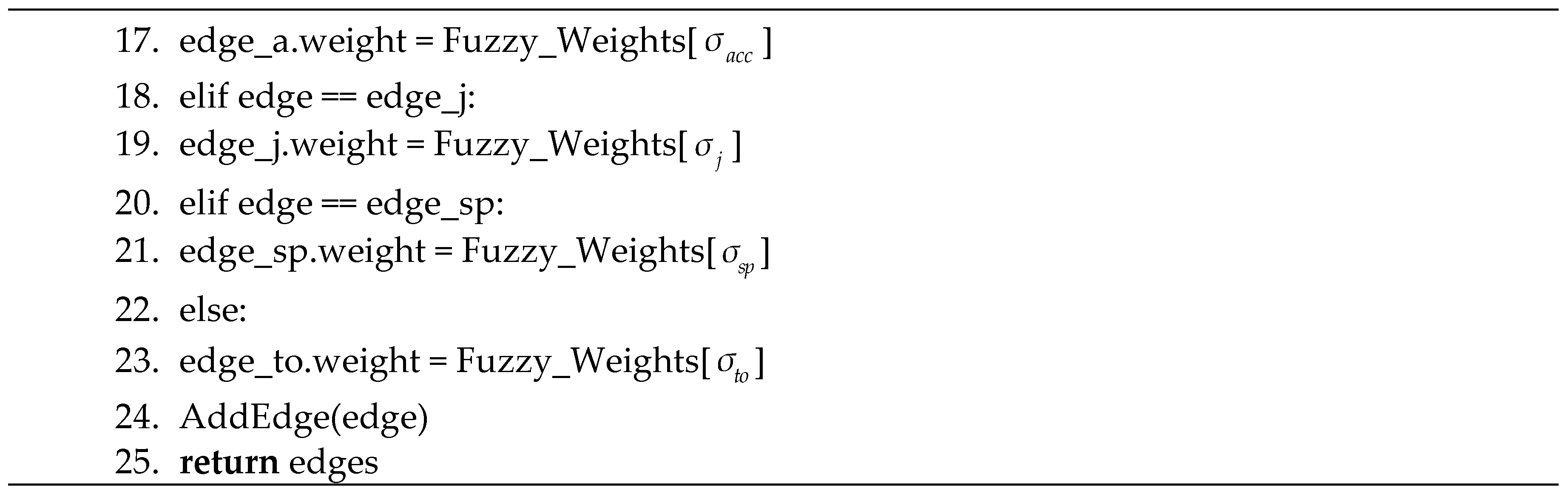
As shown in Figure 1, TEB employs a hypergraph to depict the process of solving a nonlinear optimization problem. In the figure, represents poses along the trajectory, represents waypoints, and represents associated obstacles. TEB employs different objective functions as hyperedges in the hypergraph, treating all connected poses and their time intervals as nodes in the hypergraph for optimization. The trajectory with the minimum cost under the total objective function is selected as the optimal trajectory. The TEB Optimizer section in Figure 2 illustrates the process by which TEB uses a hypergraph to optimize the trajectory.
2.2. Kinematic Model of a Car-Like Robot
At low speeds, the local path planning of car-like mobile robots is based on their kinematics without considering dynamics. The car-like robot is modeled as a rigid body with four wheels in contact with the ground, with its direction determined by the front wheels [25], as shown in Figure 3:
Figure 3 illustrates the kinematic model of a car-like mobile robot in the world coordinate system . The continuous poses of the car-like mobile robot during motion are represented as . The robot's kinematic center is the point S, located at the midpoint of the rear wheel axis. The robot's principal axis is aligned with the x-axis.
When turning, the car-like mobile robot has a rotational motion radius around the center of rotation (ICR), labeled as in the diagram; The equivalent front wheel steering angle , lies within the range. When , the robot's turning radius is equal to the minimum turning radius, . The robot's signed translational velocity along its principal axis is denoted by . The ordinary differential motion equations of the robot in the world coordinate system are as follows:
Non-holonomic constraints require that the robot's consecutive poses and lie on a common arc with the same curvature during motion [15]. As shown in Figure 4, the direction vector of the robot at pose is , which forms an angle with the velocity at , and an angle with the velocity at . The non-holonomic constraint is expressed using the following equations:
The front wheel steering angle of a car-like mobile robot has a maximum limit, beyond which the radius of the turn is minimized, referred to as the minimum turning radius. In Figure 4, the relationship between two adjacent poses can be described as:
The turning radius of a car-like mobile robot must satisfy .
TEB incorporates the non-holonomic constraint and the minimum turning radius constraint from the kinematic model of car-like robots into the total objective function in the form of weighted penalty functions, as shown in Equation:
3. Improved TEB Algorithm with Fuzzy Logic Controller
During local path optimization, the weights of the objective terms in the TEB algorithm significantly influence the actual optimization results. According to the quadratic penalty theory, the optimal solution for the original nonlinear problem can only be achieved when all the objective term weights approach infinity() [15]. Since excessively large weights can cause the solver to struggle with convergence, TEB employs a weight coefficient of 1 as the standard weight for each objective term. However, in different scenarios, the robot must consider varying priority objectives for the trajectory to reduce energy consumption and improve mobility efficiency.
Therefore, new objective for trajectory smoothness and jerkiness are added to the objective function to achieve smoother trajectories and more stable velocity changes, and a fuzzy logic control method is introduced to enhance TEB's adaptability. The flowchart for dynamically adjusting the weights of TEB objective terms using a fuzzy controller is shown in Figure 5:
3.1. TEB Objective Function Considering Robot Motion Smoothness
To address issues such as oscillations in velocity, angular velocity, and steering angles in TEB-based local path planning, smoothness and jerk [26,27] are incorporated into the TEB objective terms to reduce the robot's motion instability.
Trajectory smoothness is represented by the angular changes between adjacent pose points, as shown in Equation (10):
The Jerk is the derivative of acceleration and is calculated using the differences between four consecutive poses, as shown in Equation (11):
Therefore, penalty terms for trajectory smoothness and jerk, along with their corresponding weights, are added to Equation (9). These penalty terms are incorporated as hyperedges into the optimization framework of TEB, forming a new objective function:
3.2. Establishment of Fuzzy Rule Controller
The key to local path planning for car-like robots lies in effectively incorporating the constraints introduced by the kinematic model into the planning process. Non-holonomic constraints require replacing lateral translational motion with curved motion, while the minimum turning radius constraint further reduces the solution space for the path.
To improve the local path planning performance of car-like robots, this paper proposes using "freedom" and "directionality" to evaluate the trajectory characteristics of car-like mobile robots. Under non-holonomic and minimum turning radius constraints, the "freedom" of car-like mobile robot motion refers to the flexibility of pose adjustment, while "directionality" refers to the complexity of curved motion in the trajectory caused by non-holonomic constraints, replacing the need for lateral translation. To evaluate freedom, this paper uses the ratio of the average distance between the trajectory and obstacles to the minimum turning radius to measure the Narrowness () of the passage, which serves as an intuitive indicator of trajectory freedom; To evaluate directionality, this paper uses the proportion of different curvature arcs in the entire trajectory to quantify the turning complexity () of curved motion, which reflects the trajectory's directionality.
3.2.1. Freedom Evaluation
Due to the minimum turning radius constraint, car-like mobile robots have an inaccessible circular area on the side, and the planned path must circumvent this area. Within this area, the distance from any point to the kinematic center is , the point furthest from the robot's kinematic center is , with a distance of from the kinematic center. As shown in Figure 6, when there are obstacles outside point , the robot cannot directly turn around to move toward a target point behind it. In this situation, the robot can only adjust its initial pose and move forward in the other direction before turning to indirectly approach the target point, or adopt a reversing strategy. However, to avoid instability, reversing behavior is usually subject to strict constraints [28]. Therefore, when the distance on both sides of the robot in the passage is less than , the solution space for navigable paths is significantly reduced.
When the orientation of the target point's pose is opposite to the current pose, car-like mobile robots usually use curved motion to adjust the heading angle. As shown in Figure 7, when the space around the robot is too narrow to plan a single curved trajectory to adjust the heading angle, the robot needs to use a combination of forward and backward movements to achieve heading angle adjustment. When the distance between the obstacle and the robot, , is less than , the robot cannot adjust its heading angle by 180° using a single forward and backward combination movement, significantly increasing the complexity of pose adjustment. This limitation further reduces the solution space for path planning, constraining effective motion options.
Therefore, the adjustability of car-like mobile robot poses is evaluated using the narrowness () of the passage where the trajectory lies. is determined by the relationship between the average distance, , between all robot poses along the trajectory and the nearest obstacle, and the minimum turning radius . Assuming the semi-axle length of the car-like mobile robot satisfies , and there are n trajectory points in the trajectory, with the average distance to the nearest obstacle , is calculated as:
3.2.2. Directionality Evaluation
Due to non-holonomic kinematic constraints, the motion trajectory of car-like mobile robots requires curved motion instead of lateral translation, and an increase in curved motion raises the complexity of the trajectory. Additionally, the greater the curvature of the curved trajectory, the higher the demands on the robot's motion control inputs. Therefore, the complexity of curved motion for car-like mobile robots is evaluated using the Turning Complexity (). is derived from the proportion of trajectory segments with different curvatures relative to the total.
For each local trajectory generated by the local planner, the curvature change between each pair of consecutive poses is first calculated, where is the heading angle change between adjacent poses and , and is the length of the corresponding trajectory segment. If the curvature exceeds the turning threshold , the trajectory between and is labeled as a turning segment; otherwise, it is labeled as a non-turning segment.
Next, turning segments are identified as sharp turning segments. If the curvature of a turning segment exceeds the sharp turning threshold but is less than, the segment is classified as a sharp turning segment, where is the curvature corresponding to the minimum turning radius of the car-like robot, given by . In this paper, and . Trajectory segments identified as sharp turning segments are not counted again as turning segments. If the trajectory contains n trajectory points , it consists of n-1 segments. Let the number of turning segments be and the number of sharp turning segments be . The turning complexity is defined as:
3.2.3. Establishment of Fuzzy Rules
Fuzzy logic control is a rule-based control method. Compared to other control methods, it can simulate human reasoning through linguistic control without requiring a precise mathematical model, offering greater fault tolerance, robustness, and simplicity [29]. This paper considers the freedom and directionality of robot motion to set corresponding fuzzy logic control rules and establish a fuzzy controller for dynamically adjusting parameters.
The domain of narrowness is [0, 4], with a fuzzy set of [S, M, L]. The membership function of narrowness () is shown in Figure 9(a). The domain of turning complexity is [0, 2], with a fuzzy set of [S, M, L]. The membership function of turning complexity () is shown in Figure 9(b).); (b) Membership function graph for the complexity of turns ().
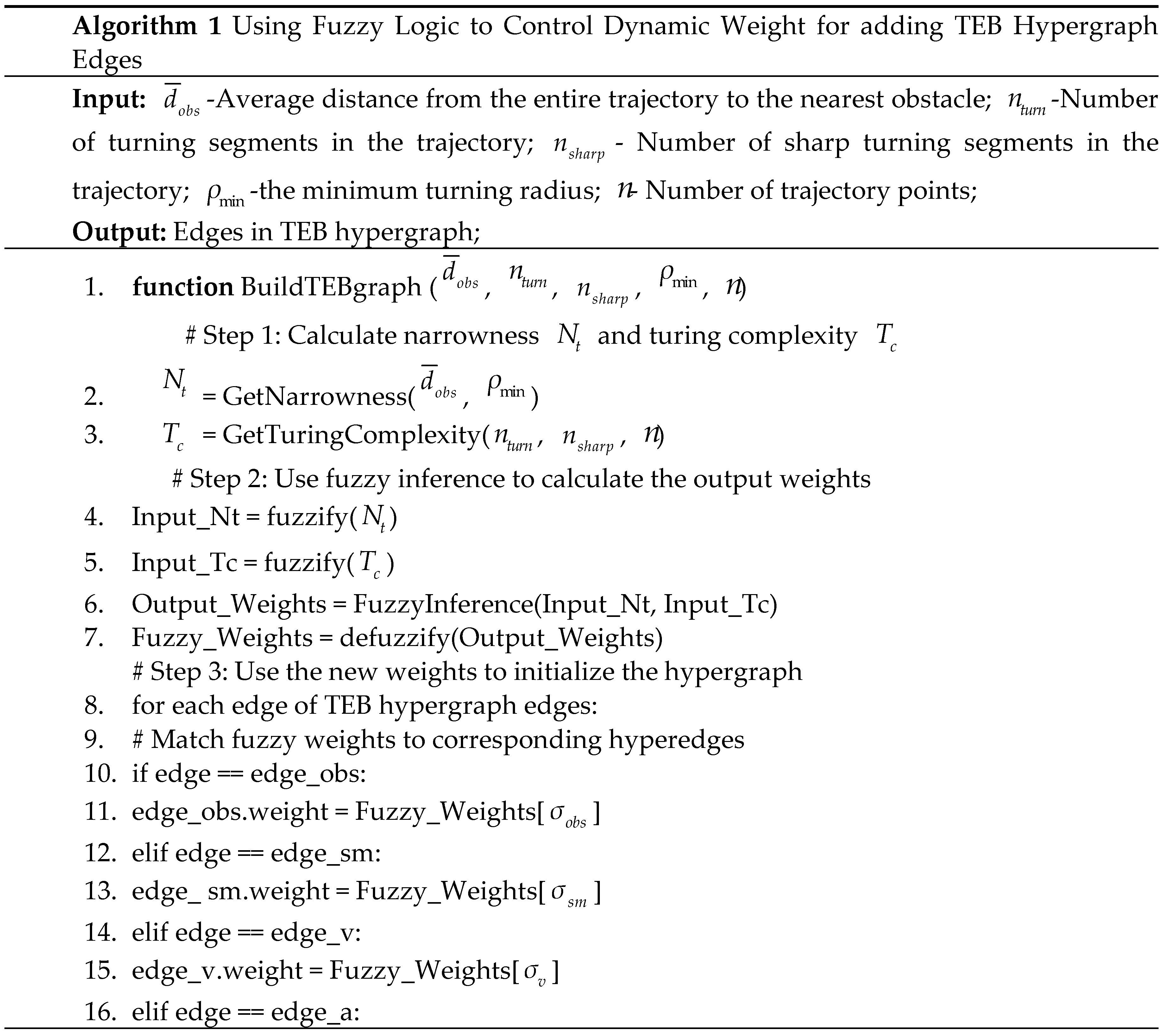
Based on the above fuzzy logic control rules, using fuzzy logic control to build TEB graph edges is as follows:
3.3. Nonlinear Mapping Strategy for Output Weight Values
The increase in penalty function weight coefficients has a nonlinear effect on optimization results, typically following a pattern close to logarithmic growth. Therefore, to simplify computation and improve the performance of the fuzzy controller, the inputs to the fuzzy controller are represented as a linear set, and a piecewise function is used to map the inputs to weight values. As shown in Figure 10, the output range of the fuzzy controller, denoted as , is [-1,3], and the real weight values, denoted as , obtained through piecewise function mapping, fall within the range [0, 1000].
The membership function for the output weights of the fuzzy controller is shown in Figure 11. The weight ranges for objectives related to obstacle distance, smoothness, velocity, acceleration, and jerk are mapped using piecewise functions. Specifically, the fuzzy output range for obstacle distance is [-1, 3], corresponding to a weight range of , with a fuzzy set of [VL,L,M,H,VH]. Since the weights for optimal time and shortest path length should not be too large, these objectives are not linearized, and their corresponding weight range is set to , with a fuzzy set of [VL, L, H, VH].
4. Simulation and Experimental Results
To validate the performance of the proposed FLC-TEB algorithm, modifications and adjustments were made to the TEB algorithm using the C++ programming language in the Ubuntu 18.04 ROS melodic environment, and comparisons were conducted with the original algorithm. First, simulation tests were conducted. The StageRos simulation environment was built to test the algorithm's ability to adaptively adjust weights in different environments, comparing the motion performance improvements brought by the new method. Next, the proposed algorithm was tested on a real car-like robot platform to evaluate its adaptive capabilities and practical improvements in robot performance. The experimental results presented in this paper are reproducible under the same robot structure and experimental parameters. In this paper, the speed smoothness metric is defined as the variance of the speed distribution along the entire trajectory. Lower variance indicates more stable speed and smoother trajectories, while higher variance suggests greater speed fluctuations and less smooth paths.
4.1. Simulation Experiment
The workstation running the program was equipped with an AMD Ryzen 5 5600H processor with Radeon Graphics, featuring 6 cores and a base frequency of approximately 3.3 GHz, and was equipped with 8 GB of RAM. The simulation employed a quadrilateral robot model to simulate a car-like robot. The robot body dimensions were 0.6m in length and 0.25m in width, with a front-to-rear axle distance of 0.4m, and a minimum turning radius of 0.5m. The kinematic parameters are provided in Table 2.
Table 3 shows the default weights for the classic TEB algorithm, the TEB algorithm optimized with smoothness and jerkiness (referred to as "Smooth-TEB"), and the weights computed for FLC-TEB in the narrow continuous turning section of Simulation Map:
Figure 12 shows Simulation Map used in this simulation. Simulation Map is a channel with continuous turns, where the width of the channel is 1.0m throughout. The car-like robot starts from the channel entrance, with the goal located at the position near the exit of the channel. The trajectory planned by the planner in a single execution on this map (red curve in the figure) is analyzed below. The kinematic characteristic curves obtained by the traditional TEB, Smooth-TEB, and FLC-TEB algorithms are shown in Figure 13.
As shown in Figure 13, in the channel environment of Simulation Map, all three Timed-Elastic-Band (TEB) algorithms generated feasible and consistent trajectories. From the perspective of trajectory length and time consumption, the TEB algorithm produced the longest path but the shortest execution time. The Smooth-TEB algorithm shortened the path by 6.25% compared to TEB, but the execution time increased by 20%. The FLC-TEB algorithm generated a path almost identical in length to Smooth-TEB but with a further increase of 23% in execution time. The comparison of data for each algorithm is presented in Table 4.
The data in Table 4 shows that, compared to TEB, FLC-TEB shortened the trajectory length by 8%, but increased the trajectory execution time by 49%. This is because the channel width in Simulation Map is very narrow, with two consecutive sharp turns near the entrance, causing FLC-TEB to increase the weight of the speed constraint, resulting in lower speeds. However, FLC-TEB reduced the change in turning angles by 50% compared to TEB and by 24% compared to Smooth-TEB. The smoothness of linear and angular velocities improved by 56%. FLC-TEB increased the weights for obstacle distance, speed, and acceleration while reducing the weights for trajectory length and execution time after considering the characteristics of the area. Notably, despite the reduced weight for trajectory length, FLC-TEB shortened the trajectory length due to better speed smoothing, indicating that FLC-TEB's weight adjustments improved the overall quality of the trajectory. Next, we analyze the motion performance of the robot moving along the complete trajectory to the destination. The kinematic characteristic curves obtained from real-time planning and full motion using traditional TEB, Smooth-TEB, and FLC-TEB are shown in Figure 14.
Table 5 shows the real-time feedback data during the complete motion process on this map. The TEB algorithm generated a longer path but had the shortest execution time. Smooth-TEB produced a path length almost identical to TEB but increased execution time by 4%. FLC-TEB generated a slightly shorter path than the other two but increased execution time by 6% compared to TEB. The results in Figure 14(a,b) shows that compared to the TEB algorithm, FLC-TEB reduced the linear velocity smoothness of the robot by 50% but increased the angular velocity smoothness by 55%. The trajectory and angular velocity smoothness optimized by the FLC-TEB planner were superior to those of TEB, enhancing motion stability and safety. This allowed the robot to reach the target point with minimal pose corrections, improving its motion efficiency.
4.2. Experiment in Real Environment
Simulation experiments cannot fully replicate the movement of robots on real road surfaces; therefore, we conducted experiments using a self-developed car-like robot platform. Figure 15 shows the robot we used, with its components listed in Table 6 and its kinematic parameters provided in Table 7.
The experiment was conducted outdoors, with multiple barriers used as obstacles. The map configuration is shown in Figure 16.
On the constructed map, TEB, Smooth TEB, and FLC-TEB were used for planning. The resulting kinematic characteristic curves are shown in Figure 17
Table 8 presents the results of this real-world experiment. From the data, it can be concluded that the FLC-TEB algorithm demonstrated significant advantages. In terms of trajectory length, FLC-TEB generated the shortest trajectory (9.41 meters), significantly outperforming TEB (11.19 meters) and Smooth-TEB (10.63 meters). This is because both TEB and Smooth-TEB required reversing to adjust the forward heading angle, whereas FLC-TEB did not encounter such situations. In contrast, FLC-TEB's trajectory duration was longer than TEB's but shorter than Smooth-TEB's. Additionally, both FLC-TEB and Smooth-TEB exhibited lower linear and angular velocities compared to TEB, indicating that FLC-TEB achieved better time results while ensuring smoother paths and velocity controls.
In terms of trajectory smoothness, FLC-TEB also demonstrated excellent performance. The average heading angle variation on its trajectory was 0.0358 rad, a 39% reduction compared to TEB (0.0504 rad). The linear velocity smoothness (0.0541 m²/s²) and angular velocity smoothness (0.0382 rad²/s²) of FLC-TEB's generated trajectory significantly outperformed TEB. It was slightly inferior to Smooth-TEB only in angular velocity smoothness. This indicates that FLC-TEB effectively reduces speed and acceleration fluctuations, improving trajectory smoothness and motion stability.
Overall, FLC-TEB not only provided shorter and smoother trajectories in path optimization but also enhanced the robot's motion stability and efficiency through reasonable time control and velocity fluctuation management, demonstrating significant advantages in practical applications.
5. Conclusions
This paper proposes a fuzzy logic-based improved TEB algorithm (FLC-TEB) for local path planning of car-like robots. The algorithm introduces constraints on trajectory smoothness and jerkiness to improve the smoothness of trajectories and the stability of velocity control inputs. It dynamically adjusts the objective function weights based on real-time evaluations of the narrowness and turning complexity of the environment, thereby enhancing trajectory quality.
- Without the fuzzy controller, the introduction of trajectory smoothness and jerkiness constraints can improve trajectory smoothness and velocity stability but at the cost of increased trajectory length and execution time;
- The introduction of the fuzzy controller significantly improves trajectory smoothness and velocity stability while adaptively adjusting the weights of the objectives based on the region's characteristics. In narrow or highly curved areas, it prioritizes improving trajectory smoothness and velocity stability, whereas in open or near-linear areas, it reduces trajectory length and execution time to achieve a better overall trajectory quality;
- Simulation results show that in narrow and continuously curved channels, FLC-TEB achieved a path length nearly identical to the classic TEB, with trajectory duration increasing by 6%, but turning angle variations decreased by 38%. Real-world experimental results further validated the effectiveness of the algorithm. In an open outdoor map with regions formed by discrete obstacles, FLC-TEB increased trajectory duration by 16% compared to classic TEB, but shortened the trajectory length by 16%. Turning angle variations decreased by 39%, linear velocity smoothness improved by 71%, angular velocity smoothness improved by 38%, and no reversing behavior was observed. These results indicate that for trajectory planning of car-like mobile robots, FLC-TEB significantly enhanced the adaptability and robustness of the TEB algorithm in complex environments.
In future work, more precise models will be considered to identify the robot's regional context, and the fuzzy sets of the fuzzy controller will be further refined to enhance the adaptability of FLC-TEB.
Author Contributions
Conceptualization, L.C. and R.L.; methodology, R.L., L.C. and D.J.; software, R.L., G.M. and S.X.; validation, D.J., R.L. and S.X.; formal analysis, G.M.; investigation, G.M. and S.X.; resources, G.M. and S.X.; data curation, D.J. and R.L.; writing—original draft preparation, R.L. and L.C.; writing—review and editing, R.L. and L.C.; visualization, G.M. and S.X.; supervision, L.C.; project administration, S.X.; funding acquisition, L.C., G.M. and S.X. All authors have read and agreed to the published version of the manuscript.
Funding
This research was funded by the Guangxi Science and Technology Major Special Program( AA23062024 and AA23062003).
Data Availability Statement
The data presented in this study are available on request from the corresponding author.
Conflicts of Interest
The authors declare no conflicts of interest.
References
- Antonyshyn, L.; Silveira, J.; Givigi, S.; Marshall, J. Multiple Mobile Robot Task and Motion Planning: A Survey. ACM Comput. Surv. 2023, 55, 35. [Google Scholar] [CrossRef]
- Dong, L.; He, Z.C.; Song, C.W.; Sun, C.Y. A review of mobile robot motion planning methods: from classical motion planning workflows to reinforcement learning-based architectures. J. Syst. Eng. Electron. 2023, 34, 439–459. [Google Scholar] [CrossRef]
- Ravankar, A.; Ravankar, A.A.; Kobayashi, Y.; Hoshino, Y.; Peng, C.C. Path Smoothing Techniques in Robot Navigation: State-of-the-Art, Current and Future Challenges. Sensors 2018, 18, 30. [Google Scholar] [CrossRef] [PubMed]
- Liu, L.X.; Wang, X.; Yang, X.; Liu, H.J.; Li, J.P.; Wang, P.F. Path planning techniques for mobile robots: Review and prospect. Expert Syst. Appl. 2023, 227, 30. [Google Scholar] [CrossRef]
- Tan, X.Q.; Han, L.H.; Gong, H.; Wu, Q.W. Biologically Inspired Complete Coverage Path Planning Algorithm Based on Q-Learning. Sensors 2023, 23. [Google Scholar] [CrossRef] [PubMed]
- Wang, W.J.; Li, J.Y.; Bai, Z.N.; Wei, Z.H.; Peng, J.X. Toward Optimization of AGV Path Planning: An RRT<SUP>* </SUP>-ACO Algorithm. IEEE Access 2024, 12, 18387–18399. [Google Scholar] [CrossRef]
- Xu, G.H.; Zhang, T.W.; Lai, Q.; Pan, J.; Fu, B.; Zhao, X.L. A new path planning method of mobile robot based on adaptive dynamic firefly algorithm. Mod. Phys. Lett. B 2020, 34, 17. [Google Scholar] [CrossRef]
- Xu, Y.Q.; Li, Q.Q.; Xu, X.; Yang, J.F.; Chen, Y. Research Progress of Nature-Inspired Metaheuristic Algorithms in Mobile Robot Path Planning. Electronics 2023, 12, 22. [Google Scholar] [CrossRef]
- Liu, Y.J.; Wang, C.; Wu, H.; Wei, Y.L. Mobile Robot Path Planning Based on Kinematically Constrained A-Star Algorithm and DWA Fusion Algorithm. Mathematics 2023, 11, 20. [Google Scholar] [CrossRef]
- Cui, X.N.; Wang, C.Q.; Xiong, Y.; Mei, L.; Wu, S.Q. More Quickly-RRT*: Improved Quick Rapidly-exploring Random Tree Star algorithm based on optimized sampling point with better initial solution and convergence rate. Eng. Appl. Artif. Intell. 2024, 133, 16. [Google Scholar] [CrossRef]
- Cao, M.L.; Li, B.X.; Shi, M.G. The Dynamic Path Planning of Indoor Robot Fusing B-Spline and Improved Anytime Repairing A* Algorithm. IEEE Access 2023, 11, 92416–92423. [Google Scholar] [CrossRef]
- Durakli, Z.; Nabiyev, V. A new approach based on Bezier curves to solve path planning problems for mobile robots. J. Comput. Sci. 2022, 58, 8. [Google Scholar] [CrossRef]
- Zhang, Y.Y. ; Ieee. In Improved Artificial Potential Field Method for Mobile Robots Path Planning in a Corridor Environment. In Proceedings of the 19th IEEE International Conference on Mechatronics and Automation (IEEE ICMA), Electr Network, 2022, Aug 07-10; pp. 185–190.
- Rösmann, C.; Feiten, W.; Wösch, T.; Hoffmann, F.; Bertram, T. Trajectory modification considering dynamic constraints of autonomous robots. In Proceedings of the ROBOTIK 2012; 2012, 7th German Conference on Robotics; p. 1.
- Rösmann, C.; Hoffmann, F.; Bertram, T. Kinodynamic trajectory optimization and control for car-like robots. In Proceedings of the 2017 IEEE/RSJ International Conference on Intelligent Robots and Systems (IROS), 2017, 24-28 Sept. 2017; pp. 5681–5686. [Google Scholar]
- Sun, X.H.; Deng, S.C.; Tong, B.H.; Wang, S.; Zhang, C.Y. A Solution for Trajectory Planning and Control of Cooperative Steering Mobile Robot Based on Time Elastic Band. J. Comput. Syst. Sci. Int. 2022, 61, 1046–1057. [Google Scholar] [CrossRef]
- Hoang, V.B.; Nguyen, L.A.; Nguyen, P.V.; Truong, X.T. A Time-Dependent Motion Planning System for Mobile Service Robots in Dynamic Social Environments. In Proceedings of the 2021 International Conference on System Science and Engineering (ICSSE), 2021, 26-28 Aug. 2021; pp. 464–469. [Google Scholar]
- Wu, J.F.; Ma, X.H.; Peng, T.R.; Wang, H.J. An Improved Timed Elastic Band (TEB) Algorithm of Autonomous Ground Vehicle (AGV) in Complex Environment. Sensors 2021, 21. [Google Scholar] [CrossRef] [PubMed]
- Zha, T.; Wen, J.; Li, Y.; Sun, L. A Local Planning Method Based on Graph Optimization Framework. In Proceedings of the 2021 6th International Conference on Control, 9-11 Oct. 2021, 2021, Robotics and Cybernetics (CRC); p. 80.
- Wang, J.Y.; Luo, Y.H.; Tan, X.J. Path Planning for Automatic Guided Vehicles (AGVs) Fusing MH-RRT with Improved TEB. Actuators 2021, 10, 19. [Google Scholar] [CrossRef]
- Smith, J.S.; Xu, R.Y.; Vela, P. ; Ieee. In egoTEB: Egocentric, Perception Space Navigation Using Timed-Elastic-Bands. In Proceedings of the IEEE International Conference on Robotics and Automation (ICRA), Electr Network, 2020, May 31-Jun 15; pp. 2703–2709.
- Liu, C.; Liu, Y. Robot planning and control method based on improved time elastic band algorithm. In Proceedings of the 2023 4th International Conference on Computer Engineering and Application (ICCEA), 2023, 7-9 April 2023; pp. 911–915. [Google Scholar]
- Nguyen, L.A.; Pham, T.D.; Ngo, T.D.; Truong, X.T. ; Ieee. In A Proactive Trajectory Planning Algorithm for Autonomous Mobile Robots in Dynamic Social Environments. In Proceedings of the 17th International Conference on Ubiquitous Robots (UR), Kyoto, JAPAN, 2020, Jun 22-26; pp. 309–314.
- Rösmann, C.; Feiten, W.; Wösch, T.; Hoffmann, F.; Bertram, T. Efficient trajectory optimization using a sparse model. In Proceedings of the 2013 European Conference on Mobile Robots; 2013; pp. 138–143. [Google Scholar]
- Vieira, R.P.; Argento, E.V.; Revoredo, T.C. Trajectory Planning For Car-like Robots Through Curve Parametrization And Genetic Algorithm Optimization With Applications To Autonomous Parking. IEEE Latin Am. Trans. 2022, 20, 309–316. [Google Scholar] [CrossRef]
- Yu, L.; Wu, H.; Liu, C.; Jiao, H.J.S. An optimization-based motion planner for car-like logistics robots on narrow roads. 2022, 22, 8948.
- Wang, Z.; Li, P.; Li, Q.; Wang, Z.; Li, Z. Motion Planning Method for Car-Like Autonomous Mobile Robots in Dynamic Obstacle Environments. IEEE Access 2023, 11, 137387–137400. [Google Scholar] [CrossRef]
- Rimmer, A.J.; Cebon, D. Planning Collision-Free Trajectories for Reversing Multiply-Articulated Vehicles. IEEE Trans. Intell. Transp. Syst. 2016, 17, 1998–2007. [Google Scholar] [CrossRef]
- Yao, M.; Deng, H.G.; Feng, X.Y.; Li, P.G.; Li, Y.F.; Liu, H.Y. Improved dynamic windows approach based on energy consumption management and fuzzy logic control for local path planning of mobile robots. Comput. Ind. Eng. 2024, 187, 18. [Google Scholar] [CrossRef]
Figure 1.
TEB uses a hypergraph to represent the nonlinear optimization problem.
Figure 2.
Timed elastic band local planner.
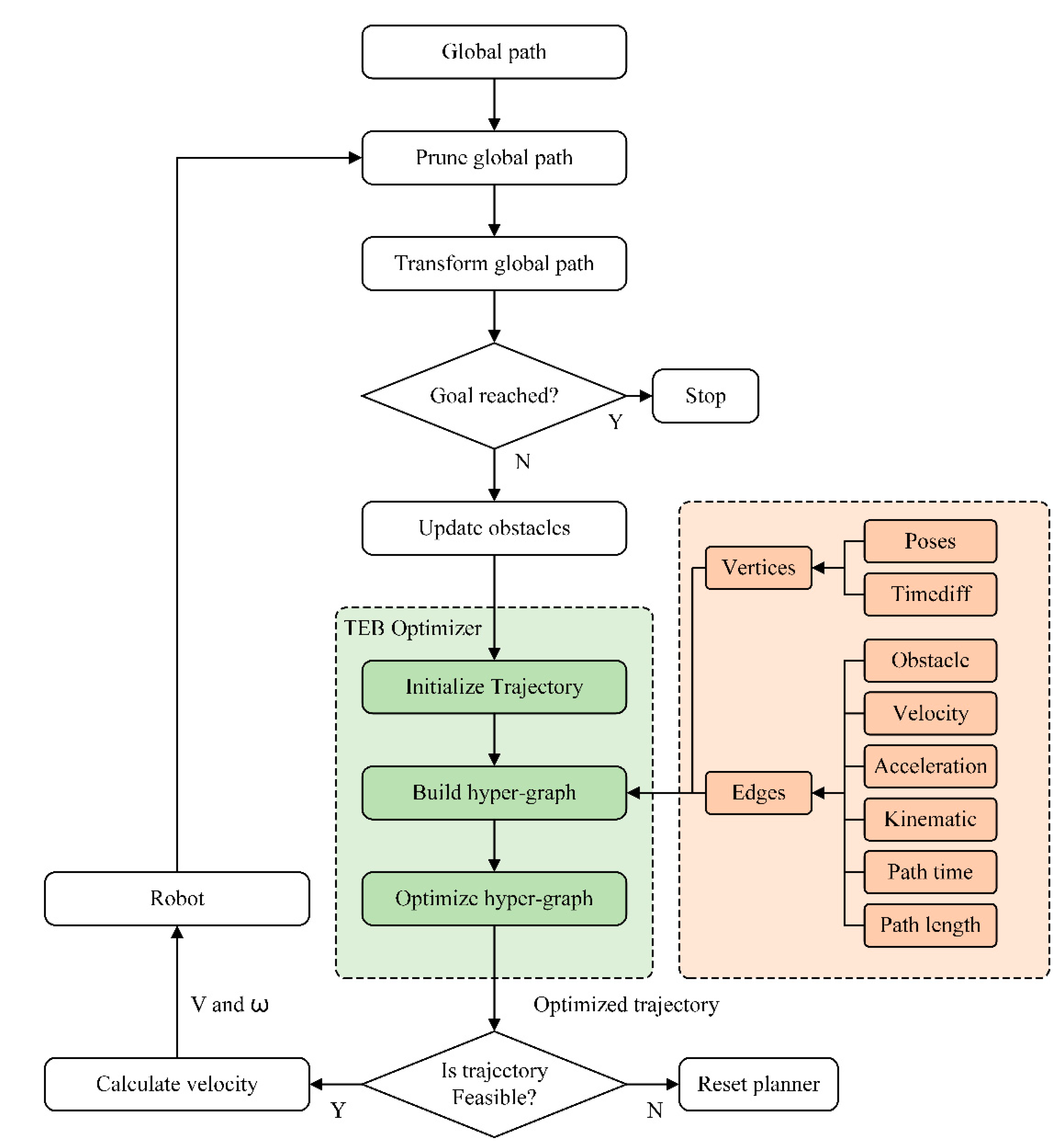
Figure 3.
The kinematic model of car-like mobile robots.
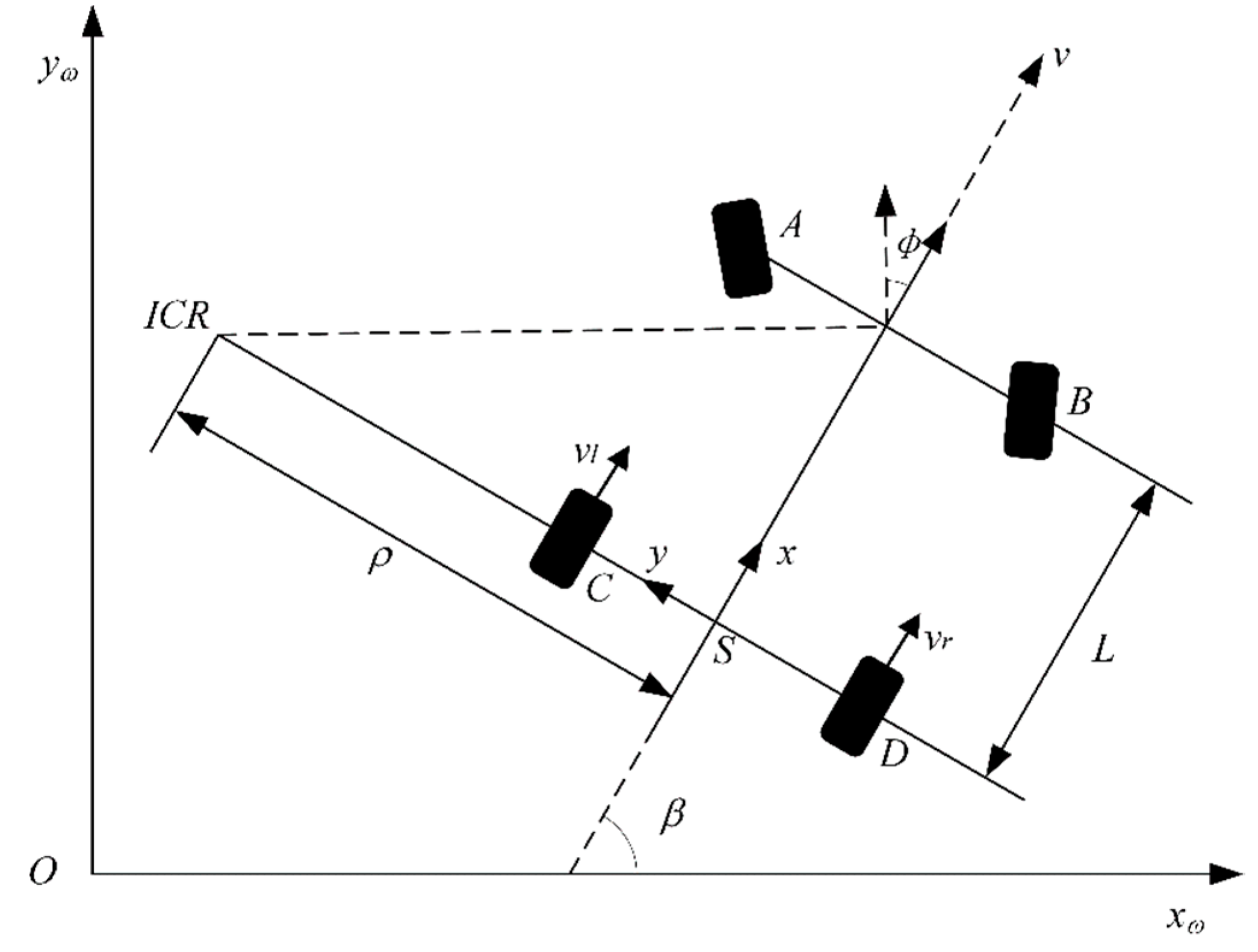
Figure 4.
Non-holonomic constraints of car-like mobile robots.
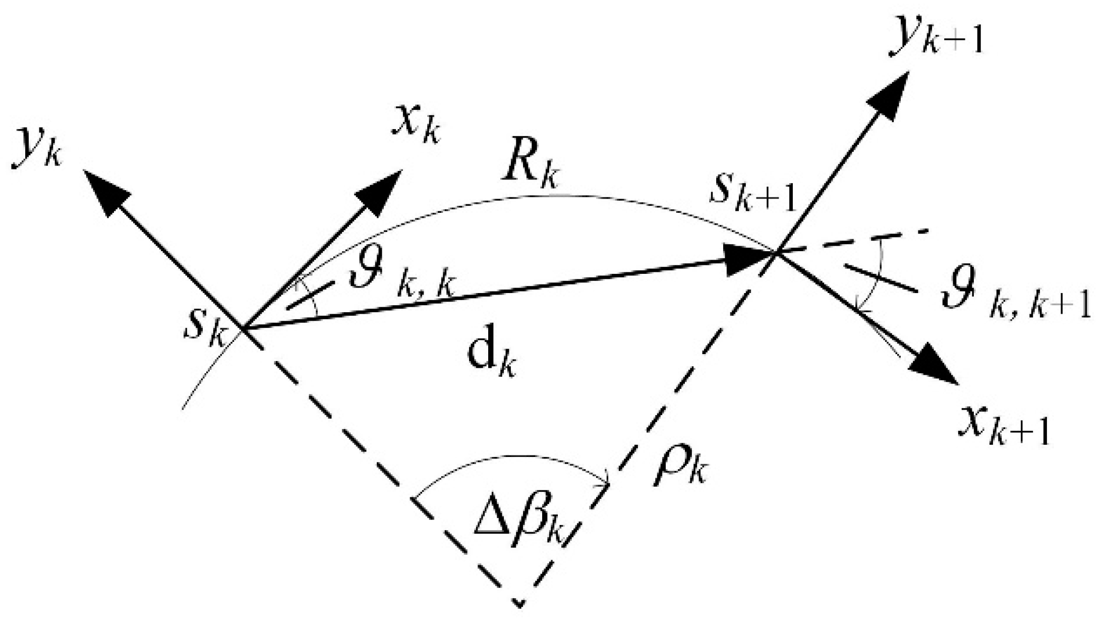
Figure 5.
TEB Algorithm Using Fuzzy Controller to Dynamically Adjust Objective Term Weights.
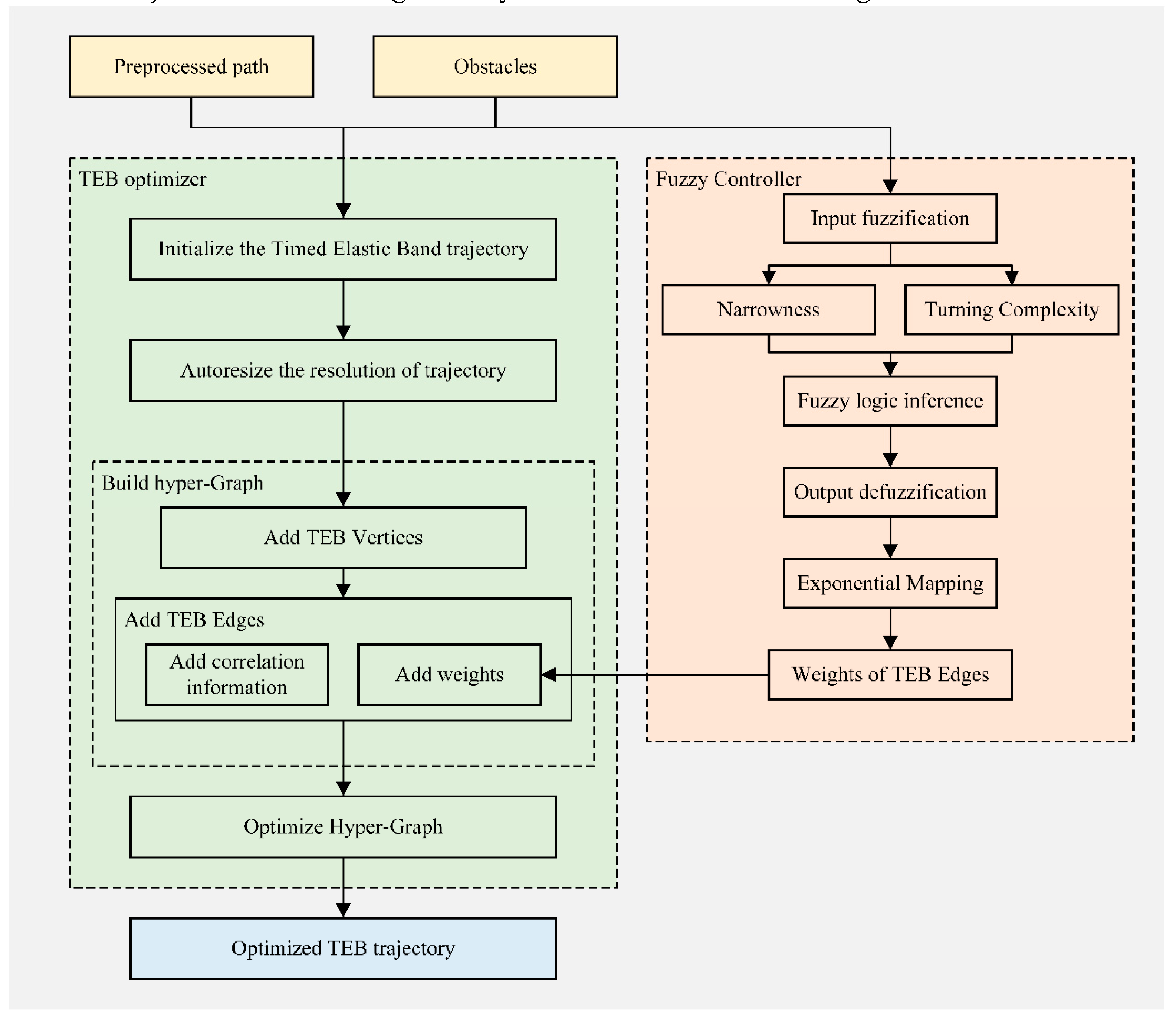
Figure 6.
The minimum turning radius limits the solution space of feasible paths for car-like robots.
Figure 6.
The minimum turning radius limits the solution space of feasible paths for car-like robots.
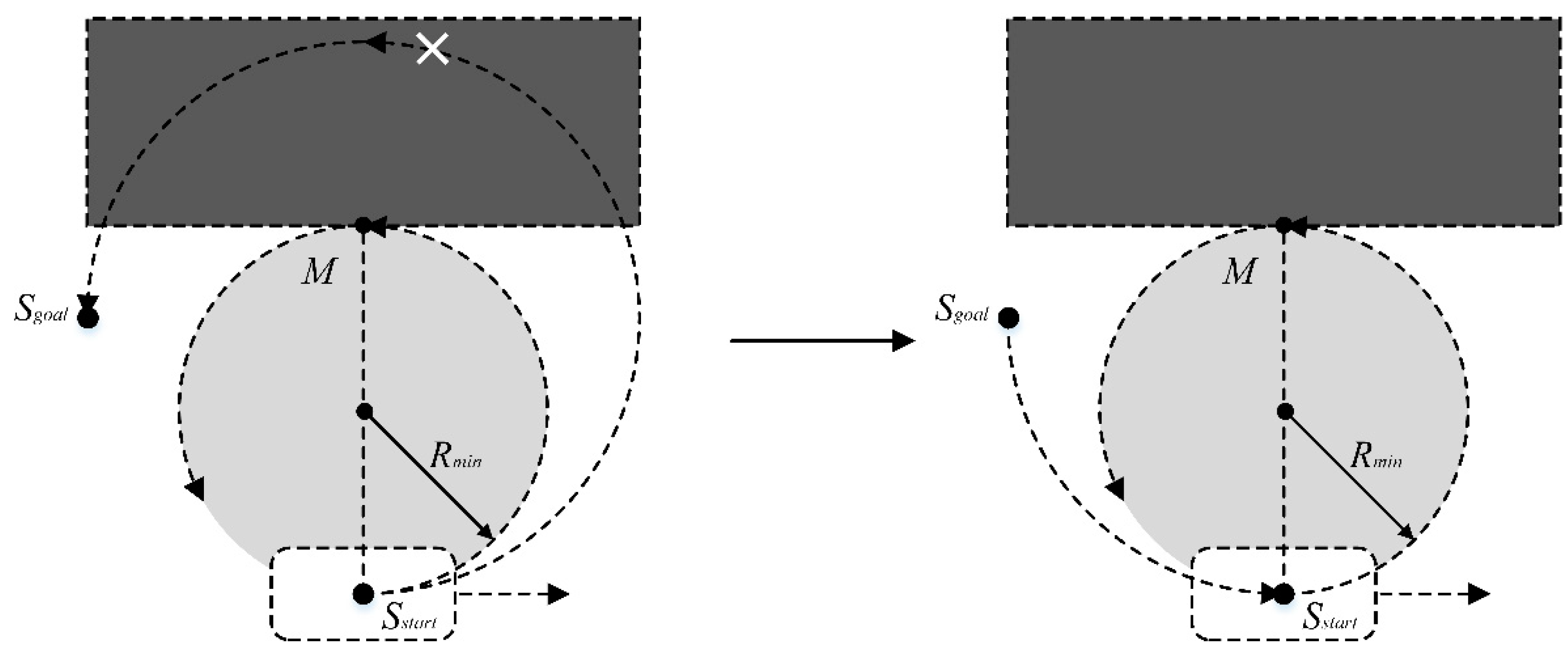
Figure 7.
The car-like robot uses a combination of backward and forward movements to adjust its orientation.
Figure 7.
The car-like robot uses a combination of backward and forward movements to adjust its orientation.
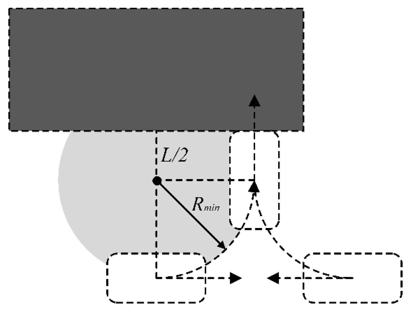
Figure 8.
A car-like mobile robot performs continuous turning movements along a trajectory.
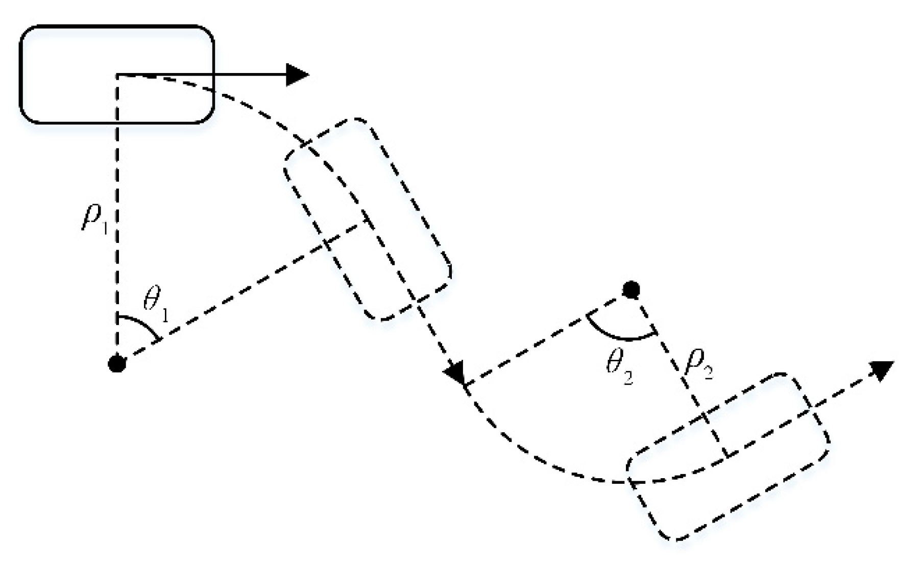
Figure 9.
(a) Membership function graph for the narrowness (
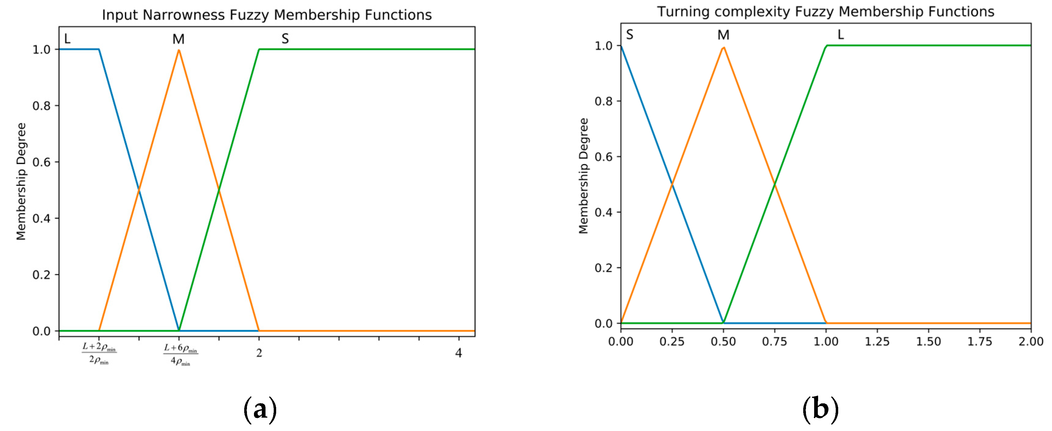
Figure 10.
Weight coefficients are mapped using piecewise functions.
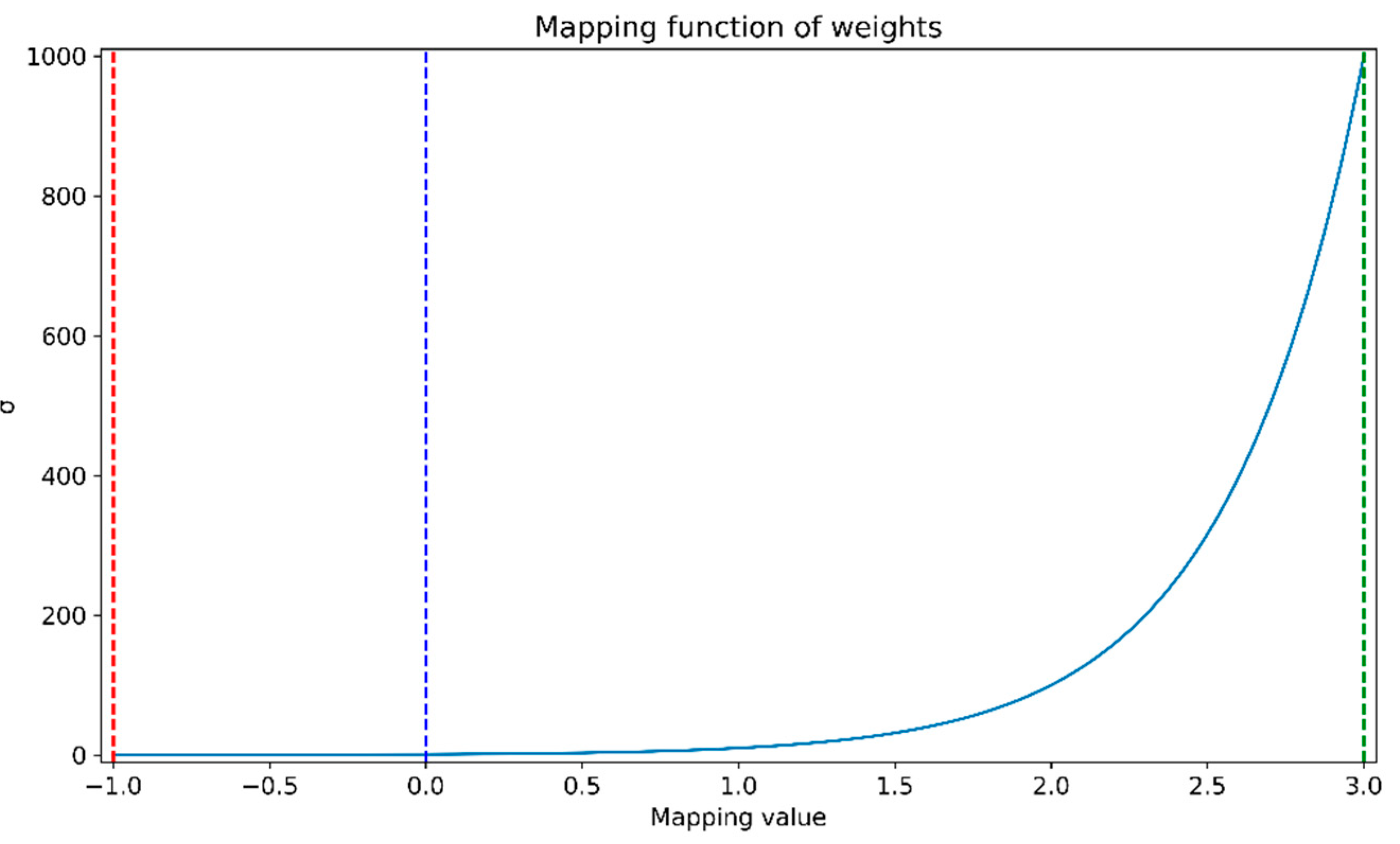
Figure 11.
Output weight membership functions: (a) Obstacle weight fuzzy membership function; (b) Smooth/velocity/acceleration/jerk weight fuzzy membership function; (c) Optimal time/shortest path weight fuzzy membership function.
Figure 11.
Output weight membership functions: (a) Obstacle weight fuzzy membership function; (b) Smooth/velocity/acceleration/jerk weight fuzzy membership function; (c) Optimal time/shortest path weight fuzzy membership function.
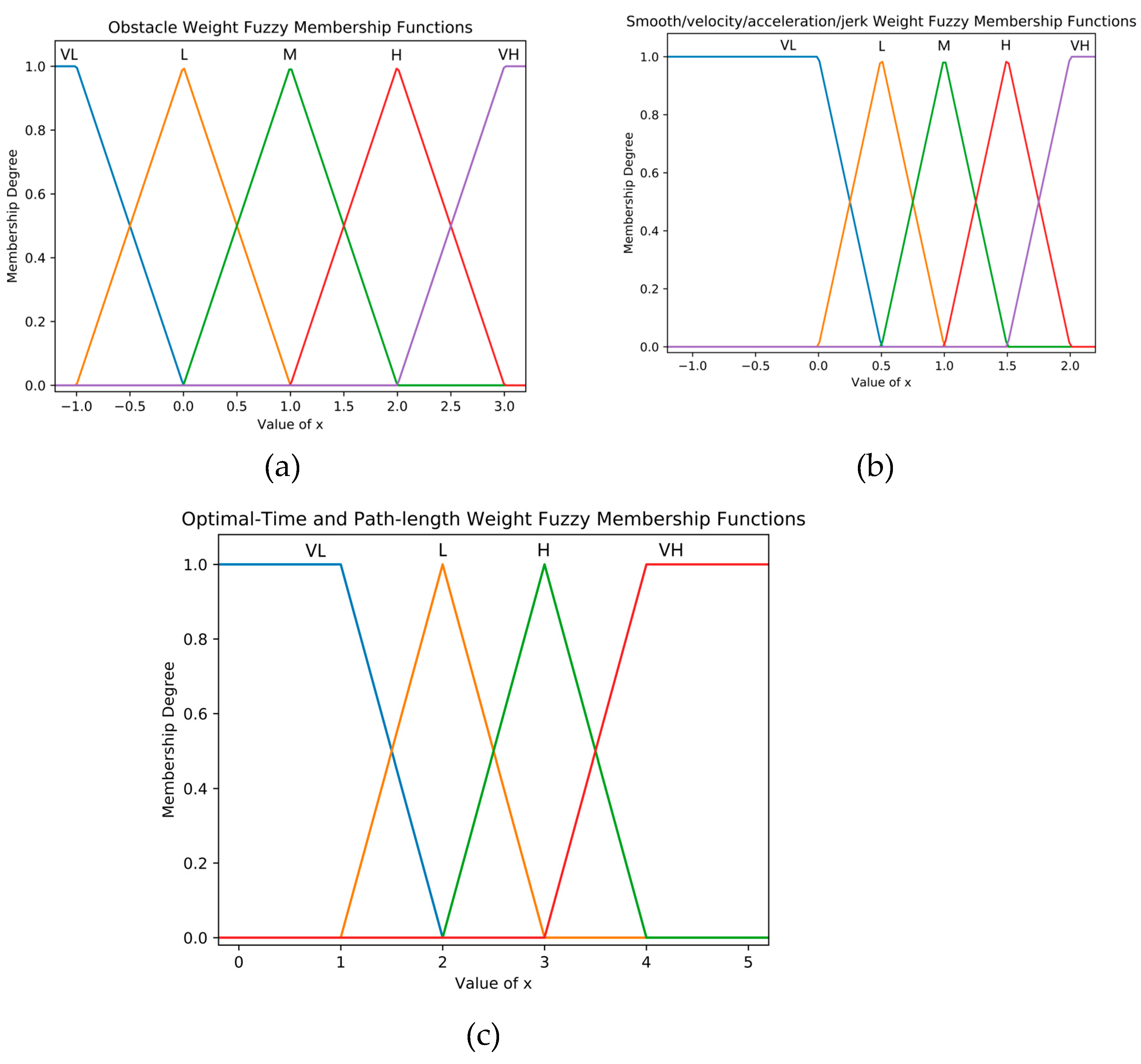
Figure 12.
A car-like robot modeled using a polygonal model moving through a narrow corridor with multiple corners. The green curve represents the global path, the red curve represents the motion trajectory, and the arrows indicate the heading angles at the trajectory points.
Figure 12.
A car-like robot modeled using a polygonal model moving through a narrow corridor with multiple corners. The green curve represents the global path, the red curve represents the motion trajectory, and the arrows indicate the heading angles at the trajectory points.
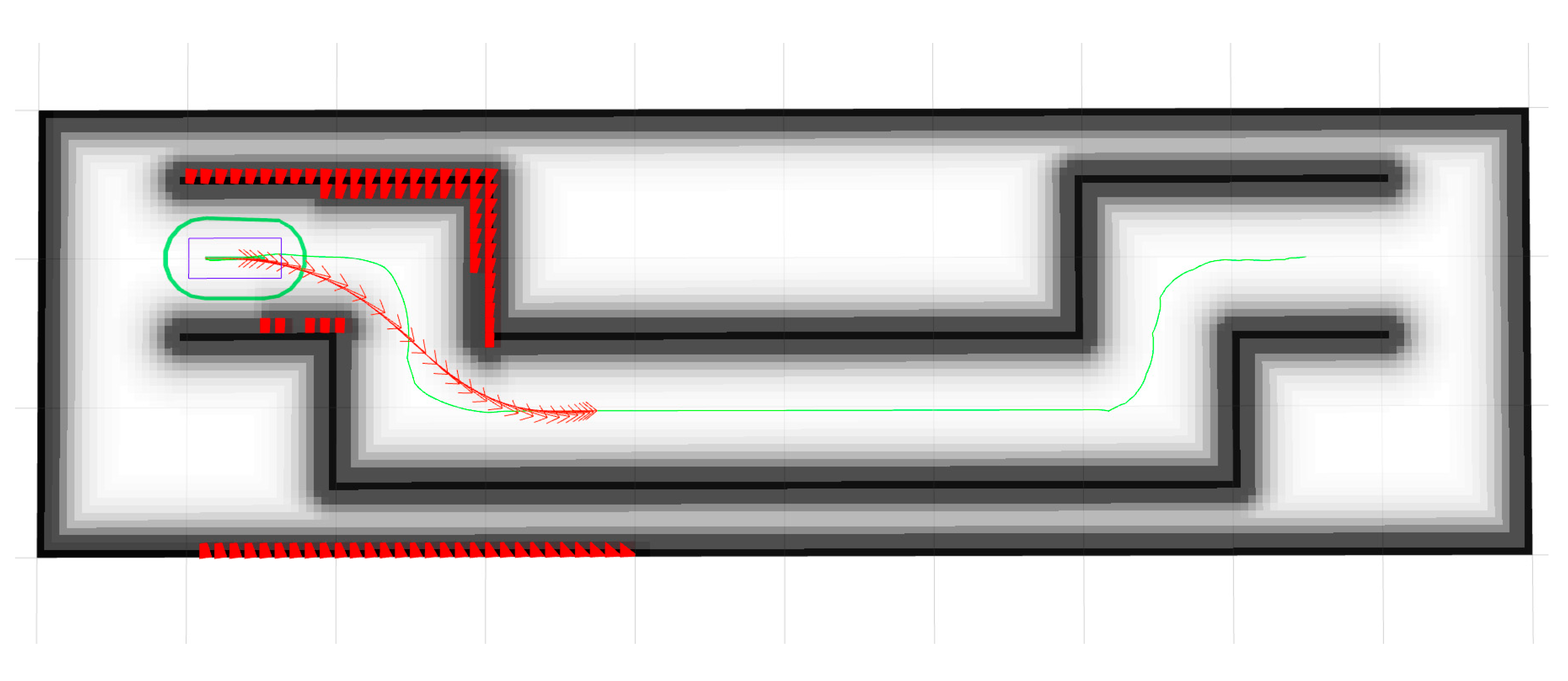
Figure 13.
Comparison of TEB, Smooth-TEB, FLC-TEB in Sim Map1:(a) Linear velocity comparison; (b) Angular velocity comparison; (c) Path comparison; (d) Path length and duration comparison.
Figure 13.
Comparison of TEB, Smooth-TEB, FLC-TEB in Sim Map1:(a) Linear velocity comparison; (b) Angular velocity comparison; (c) Path comparison; (d) Path length and duration comparison.
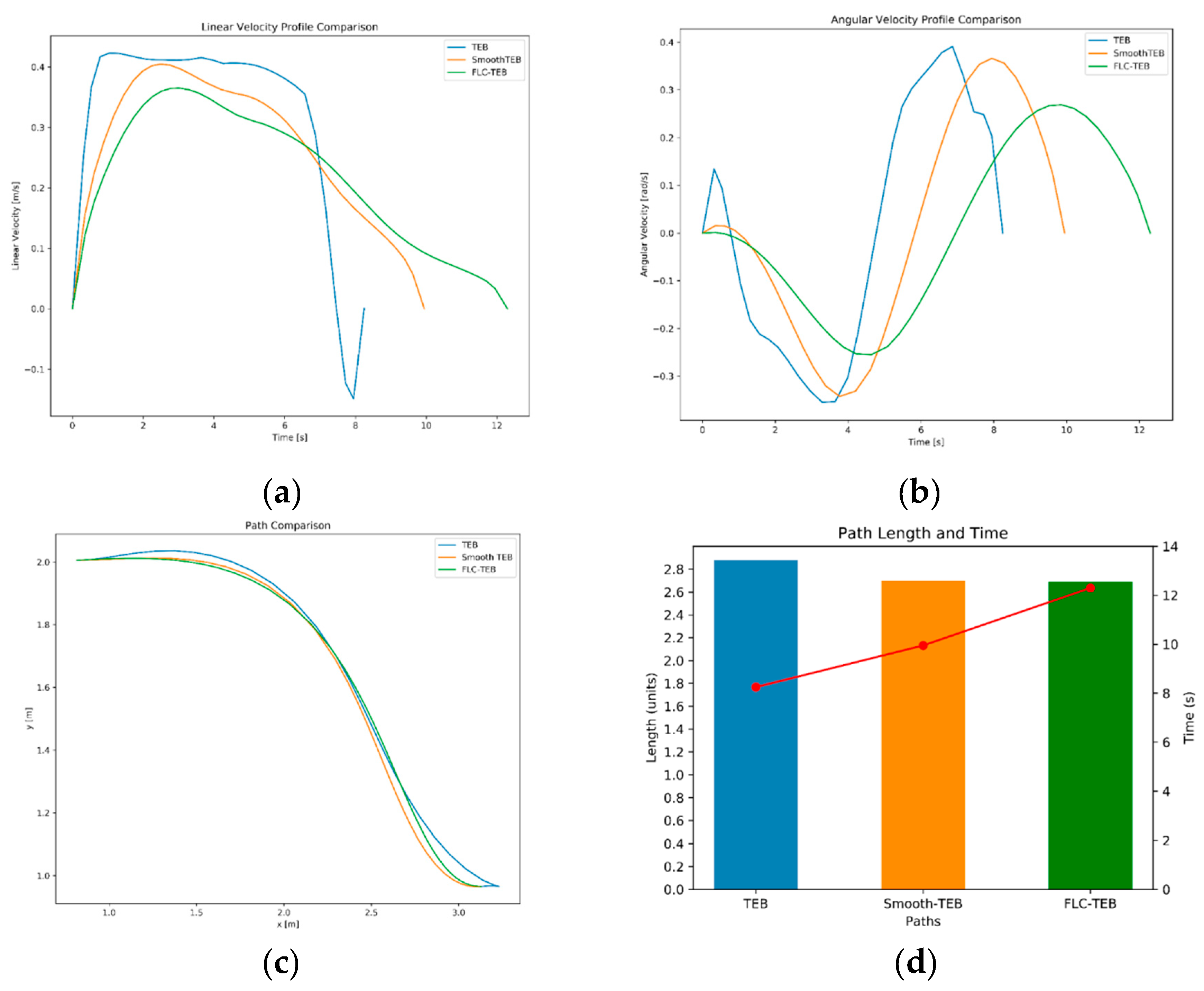
Figure 14.
Comparison of TEB, Smooth TEB, FLC-TEB in Complete Sim Map: (a) Linear velocity comparison. (b) Angular velocity comparison. (c) Path comparison. (d) Path length and duration comparison.
Figure 14.
Comparison of TEB, Smooth TEB, FLC-TEB in Complete Sim Map: (a) Linear velocity comparison. (b) Angular velocity comparison. (c) Path comparison. (d) Path length and duration comparison.
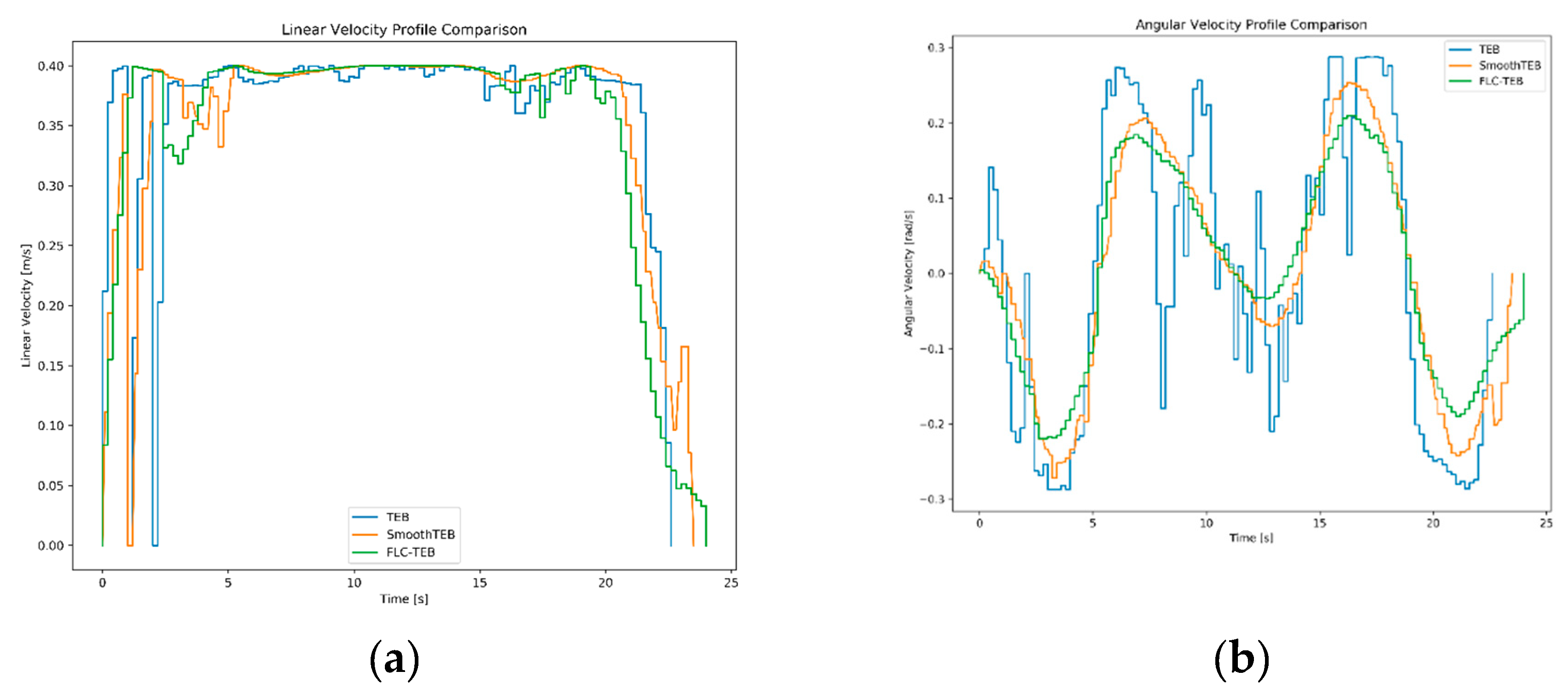
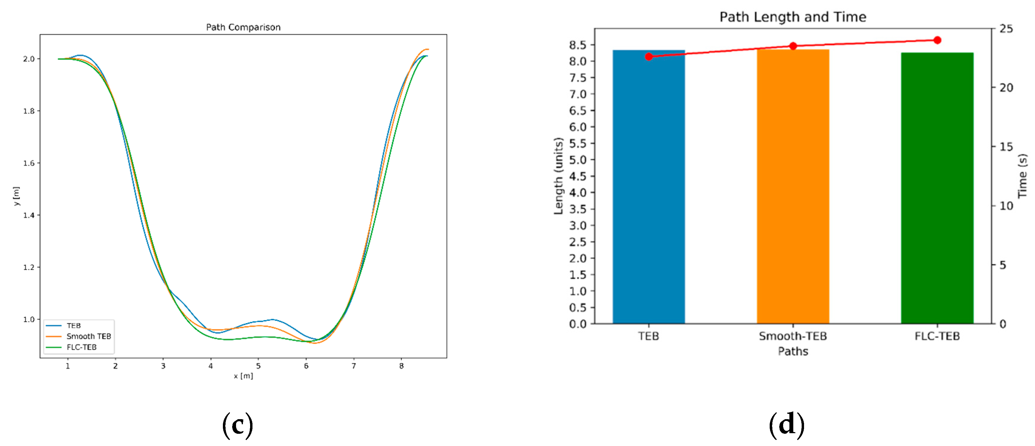
Figure 15.
The Car-like robot used in this paper.
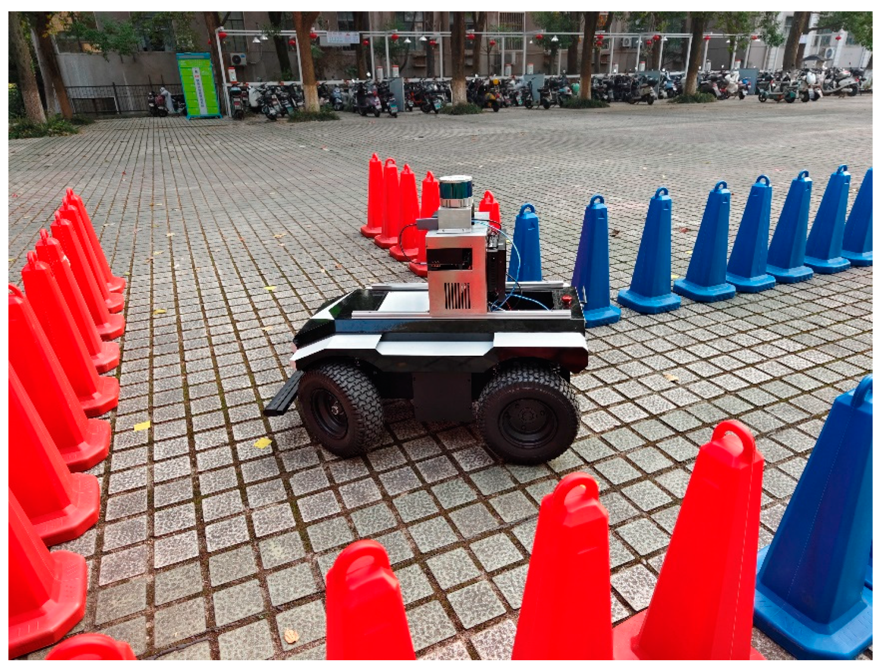
Figure 16.
Map built using SLAM in real car-like robot tests: (a) Map of an open area inside a campus. (b) The actual driving area on the map. (c) (d) Images from the real car-like robot during the test drive.
Figure 16.
Map built using SLAM in real car-like robot tests: (a) Map of an open area inside a campus. (b) The actual driving area on the map. (c) (d) Images from the real car-like robot during the test drive.
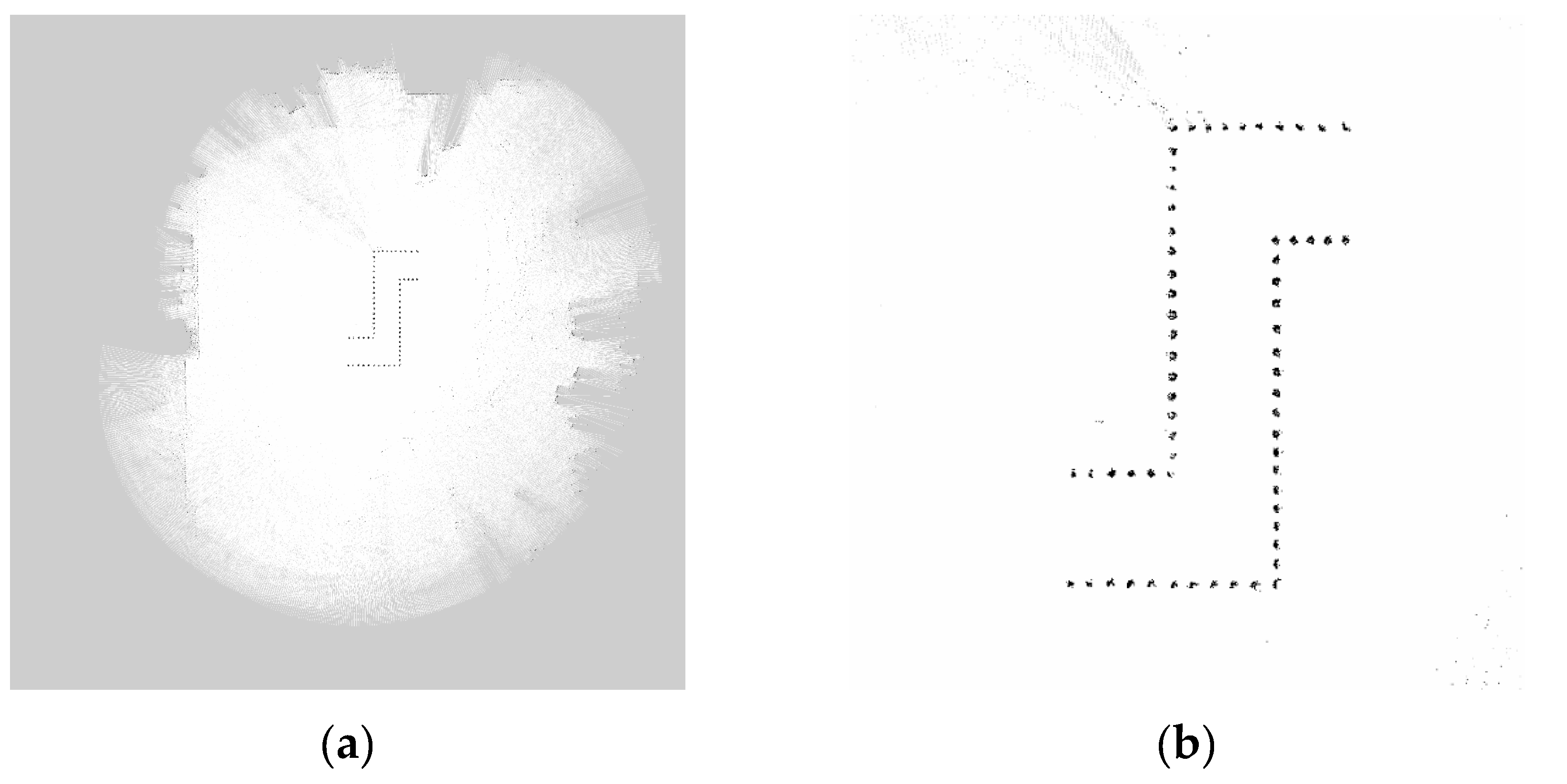
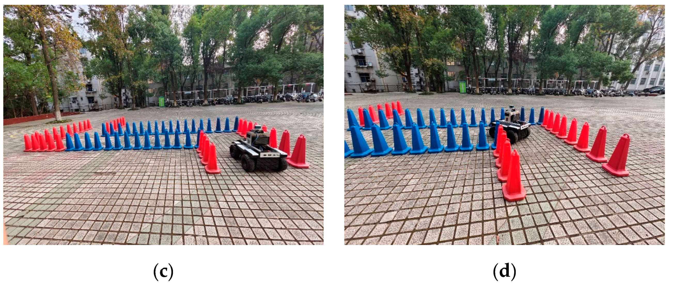
Figure 17.
Comparison of TEB, Smooth TEB, FLC-TEB in Real Car-like robot Test Map : (a) Linear velocity comparison. (b) Angular velocity comparison. (c) Path comparison. (d) Path length and duration comparison.
Figure 17.
Comparison of TEB, Smooth TEB, FLC-TEB in Real Car-like robot Test Map : (a) Linear velocity comparison. (b) Angular velocity comparison. (c) Path comparison. (d) Path length and duration comparison.
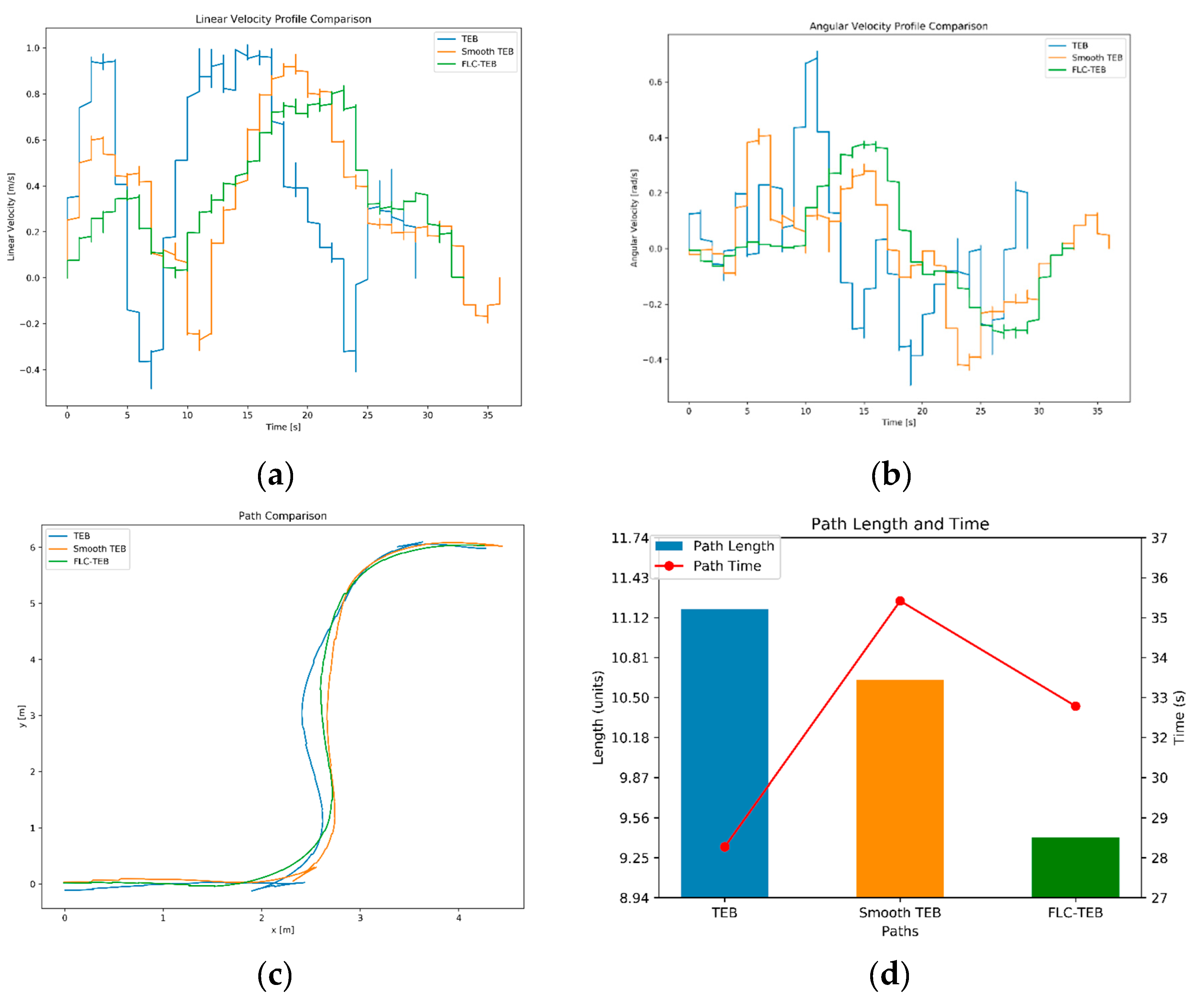

Table 1.
Fuzzy Logic Control Rule Table.
| No. | Input | Output | ||||||
|---|---|---|---|---|---|---|---|---|
| (linear) | (angular) | |||||||
| 1 | S | S | L | L | L | VL | H | VH |
| 2 | S | M | L | L | L | VL | L | H |
| 3 | S | L | M | M | L | L | VL | L |
| 4 | M | S | M | L | M | VL | L | H |
| 5 | M | M | M | L | M | VL | L | L |
| 6 | M | L | H | M | M | L | VL | L |
| 7 | L | S | H | L | H | L | L | L |
| 8 | L | M | H | M | H | L | VL | L |
| 9 | L | L | VH | H | H | M | VL | L |
Table 2.
The kinematic parameters used for this car-like robot.
| Parameters | Values |
|---|---|
| Maximum linear velocity(m/s) | 0.4 |
| Maximum linear backwards velocity(m/s) | 0.2 |
| Maximum angular velocity(m/s) | 0.3 |
| Maximum linear acceleration(m/s2) | 0.5 |
| Maximum angular acceleration(m/s2) | 0.5 |
| Maximum linear jerk(m/s3) | 0.1 |
| Maximum angular jerk(m/s3) | 0.1 |
Table 3.
Default TEB target weights and FLC-TEB calculated weights for the entry corridor section of Simulation Map.
Table 3.
Default TEB target weights and FLC-TEB calculated weights for the entry corridor section of Simulation Map.
| Weights | TEB | Smooth-TEB | FLC-TEB |
|---|---|---|---|
| Obstacle | 100.0 | 100.0 | 463.9 |
| Smoothness | 1.0 | 31.6 | |
| Velocity/Acceleration (Linear) | 2.0 | 2.0 | 31.6 |
| Velocity/Acceleration (Angular) | 1.0 | 1.0 | 10.0 |
| Jerk (Linear) | 2.0 | 31.6 | |
| Jerk(Angular) | 1.0 | 10.0 | |
| Shortest path | 1.0 | 1.0 | 0.8 |
Table 4.
Comparison of Planning Results between TEB, Smooth-TEB, and FLC-TEB.
| Trajectory performance indicators | TEB | Smooth-TEB | FLC-TEB |
|---|---|---|---|
| Trajectory length(m) | 2.88 | 2.70 | 2.69 |
| Trajectory duration(s) | 8.25 | 9.90 | 12.30 |
| Trajectory average angle changes (rad) | 0.0880 | 0.0571 | 0.0437 |
| Trajectory average linear velocity(m/s) | 0.33 | 0.26 | 0.22 |
| Trajectory linear velocity smoothness(m2/s2) | 0.0295 | 0.0144 | 0.0128 |
| Trajectory average angular velocity(rad/s) | 0.22 | 0.18 | 0.14 |
| Trajectory angular velocity smoothness(rad2/s2) | 0.0612 | 0.0464 | 0.0272 |
Table 5.
Comparison of Actual Motion Results of TEB, Smooth-TEB, and FLC-TEB in Simulation Map.
| Trajectory performance indicators | TEB | Smooth-TEB | FLC-TEB |
|---|---|---|---|
| Trajectory length(m) | 8.34 | 8.35 | 8.26 |
| Trajectory duration(s) | 22.60 | 23.50 | 24.00 |
| Trajectory average angle changes (rad) | 0.0037 | 0.0026 | 0.0023 |
| Trajectory average linear velocity(m/s) | 0.37 | 0.36 | 0.34 |
| Trajectory linear velocity smoothness(m2/s2) | 0.0053 | 0.0073 | 0.0110 |
| Trajectory average angular velocity(rad/s) | 0.17 | 0.13 | 0.11 |
| Trajectory angular velocity smoothness(rad2/s2) | 0.0381 | 0.0236 | 0.0173 |
Table 6.
Car-like robot chassis parameters.
| Components | Product Model |
|---|---|
| Industrial Control Computer (IPC) | NVIDIA Jetson Agx Xavier |
| Inertial Measurement Unit (IMU) | WHEELTEC N100 |
| Laser Detection and Ranging (LiDAR) | LSLIDAR C32 |
| Camera | Orbbec Gemini 2 |
Table 7.
Car-like robot chassis parameters.
| Parameters | Values |
|---|---|
| Wheelbase(m) | 0.56 |
| Maximum steering angle (rad) | 0.60 |
| Minimum turning radius (m) | 1.20 |
| Maximum linear velocity(m/s) | 1.00 |
| Maximum linear acceleration(m/s2) | 0.50 |
| Envelope size (m3) | 1.045×0.66×0.425 |
Table 8.
Comparison of Motion Results of TEB, Smooth-TEB, and FLC-TEB in Real Environments.
| Trajectory performance indicators | TEB | Smooth-TEB | FLC-TEB |
|---|---|---|---|
| Trajectory length(m) | 11.19 | 10.63 | 9.41 |
| Trajectory duration(s) | 28.3 | 35.5 | 32.8 |
| Trajectory average angle changes (rad) | 0.0504 | 0.0311 | 0.0358 |
| Trajectory average linear velocity(m/s) | 0.50 | 0.38 | 0.38 |
| Trajectory linear velocity smoothness(m2/s2) | 0.1757 | 0.0987 | 0.0541 |
| Trajectory average angular velocity(rad/s) | 0.19 | 0.15 | 0.15 |
| Trajectory angular velocity smoothness(rad2/s2) | 0.0607 | 0.0352 | 0.0382 |
Disclaimer/Publisher’s Note: The statements, opinions and data contained in all publications are solely those of the individual author(s) and contributor(s) and not of MDPI and/or the editor(s). MDPI and/or the editor(s) disclaim responsibility for any injury to people or property resulting from any ideas, methods, instructions or products referred to in the content. |
© 2024 by the authors. Licensee MDPI, Basel, Switzerland. This article is an open access article distributed under the terms and conditions of the Creative Commons Attribution (CC BY) license (http://creativecommons.org/licenses/by/4.0/).
Copyright: This open access article is published under a Creative Commons CC BY 4.0 license, which permit the free download, distribution, and reuse, provided that the author and preprint are cited in any reuse.


