
Submitted:
11 July 2024
Posted:
12 July 2024
You are already at the latest version
Abstract
Aiming at the APF algorithm in the collision-free path planning and LQR algorithm tracking process, there are problems such as unreachable target points, local optimization, low safety coefficient of autonomous lane change collision avoidance tracking control and poor stability, this paper proposes an optimized APF method, which solves the defects of the traditional artificial potential field method by adding the distance adjustment factor, the safety distance protection model and the sub-target virtual potential field, and at the same time generates the autonomous driving car collision-free path. The path tracking control system is designed based on feed-forward control and DLQR controller, in which the vehicle dynamics state space model is used as the basis, the model is linearized and discretized, and the corresponding constraint variables are set to minimize the control command objective cost function under the constraints, and the objective of the DLQR controller.The objective is to accurately determine the steering angle in order to achieve path tracking and eliminate the lateral error between the reference path and the actual path caused by external interference.Finally, the simulink model and CarSim parameter configuration joint simulation platform are built, and different obstacle scenarios and different speeds are selected for collision-free path planning and tracking motion simulation research and analysis, which verifies the accuracy and practicability of the algorithm, and shows more obvious advantages in obstacle avoidance ability, path smoothing degree, and collision avoidance safety stability. The ideas proposed in this paper are expected to be further extended and popularized to actual path planning problems, which has important practical significance and engineering value.
Keywords:
Path planning
; artificial potential field algorithms
; collision avoidance
; path tracking
; linear quadratic optimal controller
1. Introduction
Today, with the quick advancements in computer science, technology, and artificial intelligence, the idea of replacing human drivers with automated driving systems is slowly coming true. The development of automated driving has made it possible for people to progressively give up control [1].The integration of the Internet of Things and artificial intelligence into vehicles has enabled cars to possess their own thinking system and decision-making capabilities. Consequently, intelligent automatic driving technology in automobiles is gradually taking the role of the conventional process of “perception-decision-execution” carried out by drivers.A highly sophisticated product, automatic driving integrates a number of cutting-edge technologies, such as environment sensing, decision planning, and following control. Path planning serves as the foundation of automatic driving, while path follow, wing is a crucial technology. By implementing reasonable path planning and accurate path tracking, road safety can be ensured, traffic accidents can be avoided, passenger comfort can be maintained, and traffic congestion can be reduced [2].
Path planning has received a lot of attention in the study of obstacle avoidance for autonomous vehicles. Path design for self-driving automobiles must take into account regulations and road architecture in addition to impediments. In order to make the planned path easier for the vehicle to follow, vehicle dynamics as well as the constraints of the actuating controller are taken into account at the path planning level.Local path planning is a crucial technique for addressing the active safety issue with self-driving cars. Significant characteristics include excellent computing efficiency and real-time performance. A*, genetic, ant colony, particle swarm, and artificial potential field (APF) methods are currently the most common local path planning algorithms. The potential field is created using the artificial potential field method based on the potential functions of objectives, road constructions, and barriers. It moves along the potential field’s downward direction as it plans the route. The route tracking module then figures out the inputs needed from the vehicle to track the path.Its cheap computational cost, even for complicated path planning including barriers and road features, is this method’s key benefit over other path planning approaches. It benefits from quick searches, tremendous computational power, and simple modeling. In contrast to other algorithms, the approach is also well suited for active obstacle avoidance in self-driving automobiles [3]. The topology of the actual driving environment of the vehicle is constructed using the corresponding gravitational and repulsive potential field values, which are formed around the obstacles, in accordance with the traditional artificial potential field method.The conventional APF-based vehicle active obstacle avoidance path planning method does, however, have some drawbacks. The standard APF-based self-driving vehicle is unable to get information about the state of the world’s roads [4]. The conventional APF-based vehicle active obstacle avoidance path planning method does, however, have some drawbacks. The standard APF-based self-driving vehicle is unable to get information about the state of the world’s roads.An extensive body of research has been done on APF-based path planning and tracking. In order to enhance the obstacle avoidance function and enable the planned courses to suit the various requirements of vehicle travel.Tang Zhirong et al. [5] ellipticized the distances in the conventional repulsive potential field. To address the local minimum problem, An,L et al. [6] suggested a novel obstacle point construction approach. To increase the planning path’s smoothness, Xiu Caijing et al. [7] coupled the vehicle restrictions with the objective function. The strategy, however, is only able to address the vehicle path planning problem in static environments; it ignores the path planning problem in dynamic environments, making it challenging to use in automatic driving. The approach is straightforward in theory and performs well in real-time. In real applications, however, it is simple to run into issues with local optimal solutions and goal unreachability due to a lack of constraints like vehicle dynamics. The resilience of the algorithm is impacted by the parameters [8].
X. Song et al. [9] By deciding on a strategy to enhance the heuristic of the search and increase the applicability of the algorithm improved the smart droplet algorithm. [10] Wang, X., Liu, M., and Ci, Y. offered a technique to provide advice for corrective speed, reducing the detrimental effects of finite rationality.Jian, L. et al. [11] refined the ant colony algorithm by combining it with the artificial potential field approach for global and local planning, respectively.To increase the algorithm’s viability, Liu et al. [12] integrated the artificial potential field method with the composite force field to relocate the sampling sites with a tendency for collusion to the region of no collusion.In order to overcome the shortcomings of the APF algorithm, such as its propensity to easily fall into local minima.For virtual impediments, Zheng et al. [13] introduced a new minimal criterion and improved the local path planning method.The local minimization problem was resolved by Matoui [14] and colleagues using a non-minimum speed approach.To solve the local minimization problem brought on by obstructions near the target, Ning et al. [15] suggested a safe distance. A better active filter was then used to design an obstacle avoidance controller.
Path tracking control is a critical technology for self-driving cars, and it is primarily implemented by active steering or differential braking [16]. The route tracking problem of self-driving cars has been explored by relevant researchers using proportional integral differential (PID) control [17]. Linear self-resistance control [18], pure track model, fuzzy adaptive control [19], model predictive control [20], and other methods are used. However, because differential braking affects the longitudinal motion of the vehicle, as well as the complexity and uncertainty of the subsequent path of high-speed vehicles, real-time path tracking function realization is currently facing technical challenges under complex working conditions. Under complex working situations, active steering now confronts technical challenges. The employment of model predictive control methods can increase control performance by maximizing the objective function while also taking the vehicle’s kinematics and dynamics into account.To construct predictive control for tracking yaw stability, Zhou Li-Hua et al. [21] adopted the linear quadratic regulator (LQR) technique.Lina Wu et al. [22] proposed a new strategy based on MPC and connected vehicles (CVs) for metering and speed guidance control of urban highway entrance ramps. To achieve adaptive optimization of predictive views, Hai Wang et al. [23] suggested a model predictive control route tracking method based on variable predictive views. Morales S et al. [24] devised an omnidirectional configuration to realize trajectory tracking and combined the multilevel control method into a linear quadratic regulator trajectory tracking controller to reduce trajectory tracking error.In the study of route tracking control method, Chen, J et al. developed a linear time-varying model predictive control (LTV-MPC) method and assessed the selected control parameters on the path tracking control method. The impact of this algorithm’s processing speed comes from a variety of sources. The underlying logic and essential objective of path tracking for driverless vehicles can be inferred to drastically reduce the path error between the actual route and the expected route throughout the autonomous driving process. Pure tracking control, linear quadratic regulator control, and model predictive control are the current major route tracking control approaches.
Based on the aforementioned study, the standard artificial potential field approach is enhanced in this paper to address the target unreachability issue by including a distance adjustment factor and a safe distance protection model. To facilitate a better resolution of the local minimum problem, a virtual sub-target potential field is introduced.In order to assure the practicality and correctness of path planning in dynamic situations, a dynamic road repulsive potential field based on the safety distance protection model is constructed for road structures in dynamic environments.Compared with literature [xii], by introducing new potential field models and optimization algorithms, improved artificial potential field method can more effectively guide autonomous vehicles to avoid obstacles and improve obstacle avoidance efficiency and safety. And it has higher adaptability and better handling of dynamic obstacles, such as moving vehicles or pedestrians, which is very important for autonomous vehicles to operate in the real environment. It also has better path planning ability, which can more accurately plan the vehicle’s traveling path and avoid the problem that the path is unreachable or trapped in the local optimal solution. Better real-time and stability, can respond quickly in a real-time environment, and can stably handle a variety of complex obstacle avoidance situations. Then, to design the right path, apply the enhanced artificial potential field approach and establish the vehicle dynamics model based on the bicycle model principle, by linearizing and discretizing the model and constructing the path tracking model, and use the corresponding constraint variables to establish the optimal objective function of predictive control and under the constraints.The objective cost function of the control command is minimized under the constraints.Finally Joint simulation is performed using MATLAB and embedded simulink model and CarSim. The experimental results show that the controller has strong obstacle avoidance ability and tracking performance under different dynamic obstacle scenarios and different speed parameters, and the variation of each parameter is within a reasonable range, with better driving safety and stability.
2. Collision Avoidance System General Architecture
2.1. Collision Problem Description
Vehicle collisions are the primary cause of most traffic accidents. Any collision avoidance system’s objective is to create a vehicle control algorithm that will prevent an oncoming collision. There are two conceivable options for collision avoidance maneuver driving configurations: longitudinal control and lateral control.
Currently, emergency brake aid or brake assist systems are being installed in an increasing number of cars. However, longitudinal collision avoidance controllers are only partially effective in avoiding head-on collisions on the road between fast-moving vehicles or rear-end crashes when there is not enough space between the vehicles. In order to drive the vehicle away from the obstacle collision hazard and since lateral vehicle maneuvering can be completed in less time than stopping, aggressive lateral vehicle maneuvering is more appropriate.By accurately calculating and adjusting the vehicle’s steering angle in real-time, autonomous driving systems can achieve more precise and accurate lateral control, which enhances the stability and safety of the drive. In this situation, autonomous driving systems can sense road conditions and obstacles in real-time and make steering decisions quickly and accordingly. In this study, we concentrate on leveraging lateral control of self-driving vehicles to perform obstacle avoidance maneuvers and track obstacle avoidance planning paths with benefits such as stability, comfort, and relevance to real-world settings.
2.2. Collision System Framework
The suggested collision avoidance framework seeks to maintain the vehicle as closely as feasible to the intended path while generating collision-free paths under various obstacle scenario conditions. To accommodate changes in obstacle placements and velocities in various obstacle scenario conditions, the routes are changed within the same control cycle. The system is made up of three modules: a virtual environment model simulation, a path tracking control system, and a collision-free path creation module.According to the potential field method, which is a local path planning algorithm based on a virtual force field proposed by Khatib in 1985, vehicles traveling on roads can be planned under various obstacle scenarios. The algorithm’s basic idea is to assume that the traveling target point generates a gravitational force on the vehicle and the obstacle generates a repulsive force on the vehicle, and the vehicle is controlled to travel along the potential field.The algorithm’s fundamental notion is that the vehicle is controlled to move through the “potential valley” between the “potential peaks” in the potential field, assuming that the traveling goal point creates gravitational force on the vehicle and the obstacle generates repulsive force. While the repelling force is inversely proportional to the distance between the vehicle and the obstacle, the gravitational force is proportionate to the distance between the vehicle and the traveling target point.By calculating the combined gravitational and repulsive forces acting on the vehicle as an external force, the vehicle’s motion direction and speed may be controlled. The obstacle vehicle pushes the primary vehicle away, as seen in Figure 1. The target point also generates an attracting force for the primary vehicle. The main vehicle moves in the direction of the combined force as a result of the combined action of the attracting and repulsive forces.The primary vehicle then avoids the obstacle vehicle using the obstacle avoidance system’s frame control, arriving at the target place in the end. The technique is a feedback control approach that is simple to mathematically explain, quick to react, and easily realizes the benefits of the algorithm and the environment to build a closed-loop control, among other things. The intended path is often smooth and safe, with a certain level of robustness.
3. Path Planning for Autonomous Obstacle Avoidance Based on an Improved APF algorithm
3.1. Road Potential Field Model
For autonomous driving to be safe, modeling an accurate and secure road boundary potential field function is crucial. It is assumed that the route that the primary vehicle drives on has two lanes, as illustrated in Figure 1.On the right and left sides of the road, respectively, are dispersed A and B. Let lane B serve as the travel lane, while lane A serve as the overtaking lane. The road coordinate system’s horizontal and vertical coordinates are x and y, respectively.In order to avoid a collision and keep the vehicle safe, the main vehicle should overtake any obstacle vehicles on the road, as shown in Figure 1, in accordance with the design principle of the active obstacle avoidance system for self-driving vehicles. In order to prevent more serious traffic collisions, the primary vehicle should also stay off the edge of the boundary and outside the boundary on both sides of the road.
3.1.1. Hazardous Potential Fields at Road Boundaries
The roadway lateral hazard potential field as a function of Px with x-direction is expressed as:
The longitudinal hazard potential field of the road as a function of the x-direction, Pz, is expressed as:
The longitudinal hazard potential field of the road as a function of the y-direction, Py, is expressed as:
where (X0, Y0) are the obstacle coordinates, Db is the main vehicle safety distance and Dt is the transition region. The function Ur of the road hazard potential field is expressed as:
The expression for the lateral repulsion of the road is:
The expression for the longitudinal repulsive force on the pavement is:
The attraction potential field expression Uatt is:
where Ds denotes the distance range of the vehicle forward path search, Xr denotes the center line of the overtaking lane. yv is the longitudinal position of the center of mass of the main vehicle in the coordinate system.
The roadway lateral gravitational force expression Fxatt is:
The roadway longitudinal attraction expression Fyatt is:
3.1.2. Safe Distance Protection Model
Vehicle braking, steering, and road structural parameters need to be taken into account when building the obstacle vehicle potential field. Additionally, it’s crucial to guarantee that the primary vehicle has enough time to make decisions regarding steering behavior and high stability when performing active obstacle avoidance maneuvers.
For active obstacle avoidance, it is therefore important to make sure that the safety distance Db and transition distance Dt are at least:
where v1 and v2 are the initial speeds of the main vehicle and the obstacle vehicle on the road, Fm is the maximum braking force of one wheel, M is the total mass of the main vehicle, and L1 is the length of the body of the obstacle vehicle.
3.2. Traditional Artificial Potential Field Method
3.2.1. Target Point Gravitational Field
Figure 2 (a) shows the traditional artificial potential field method’s gravitational field function is:
where X is the autopilot vehicle’s position vector, Uatt is the gravity potential field at the target location, Katt is the gain coefficient of the gravity potential field, which is a positive real number, and Xg is the autopilot vehicle’s target position vector.The gravitational potential field’s negative gradient is discovered:
3.2.2. Obstacle Vehicle Repulsion Field
Figure 2 (b) and (c) shows the expression for the specific potential field function of the repulsive force nature potential field is:
where Urep is the obstacle vehicle repulsive force field; Krep is the repulsive potential field gain coefficient, a positive real number, D is the straight line between the car and the obstacle vehicle shortest distance; D0 is the obstacle vehicle repulsive force can affect the maximum range.
3.3. Optimization of the Artificial Potential Field Method
3.3.1. Repulsive Potential Field Function with Increased Distance Adjustment Factor
This paper suggests an improved repulsive potential field function based on the original one, increasing the distance adjustment factor to reduce the repulsive force on the vehicle at the target point in order to address the unreachable target issue of the artificial potential field method. The following is the enhanced repelling potential field function:
where [x, y] are the autonomous vehicle’s real-time coordinate points; [xg, yg] are the coordinates of the target point; and R is the radius of the autonomous vehicle.
You may determine the repelling force of the obstacle vehicle’s potential field by:
From Eqs. (3) and (16), the repulsive potential field changes only when it is close to the target point. However, the improved method reduces the search efficiency of the algorithm. [25] Therefore, in this paper, the repulsive force is improved, i.e., the distance adjustment factor is added to the original repulsive force. The repulsive force formula is:
Eq. (16) not only enhances the repulsive potential field to make sure that the vehicle’s repelling force tends to zero at the target point, but also accounts for the self-driving car’s body radius to make the path more dependable and safe. The traditional potential field function’s target unreachability issue is resolved by the improved potential field function, which also eliminates the improved repulsive force extremum and prevents situations where there is an excessive amount of repulsive force.
3.3.2. Subtarget Virtual Point Intervention
After confirming that the primary vehicle is entrapped in the local minimum, the decision of the virtual target point’s position must be taken into account. First, care must be taken to prevent the inclusion of this point from causing it to mix with the gravitational or repulsive force and imprison the primary vehicle once more in the local minima. Second, in accordance with the active obstacle avoidance system for vehicles’ design principle, the primary vehicle shall attempt to maintain lane centerline during actual driving. In other words, the main vehicle should preferentially reach the center of the neighboring lane when engaging steering obstacle avoidance behavior.As a result, lane B’s centerline should be set at point P1’s horizontal coordinate X1. When the main vehicle enters a localized minimal point, point P1 should also guarantee that it can be subjected to a significant attractive potential energy.Figure 3 shows that the primary vehicle can then successfully execute active obstacle avoidance and fast get rid of the local minima. In conclusion, the virtual target point’s coordinates are set as , and then, using the spatial geometric relationship, the minimum distance between the virtual target point P1 and the main vehicle’s center of mass is calculated as:
3.3.3. Subtarget Virtual Potential Field Attraction Function
To ensure that the newly introduced virtual target point may successfully address the local minima problem, we provide an appropriate attractive potential field function. This feature must be able to rapidly activate and operate as the main influencing factor in the event that the main vehicle gets trapped in a local minima. The gravitational potential field function of the second virtual target can be expressed by the following formula:
where Kvir is the field gain coefficient for the attraction potential.
The gravitational potential field’s negative gradient, or Fvir is the associated potential field force. In order to express the second virtual target gravitational potential field force F bundle, the following functions are used:
The host vehicle was pointed in the direction of the second virtual potential field force. After the current problem of falling into the minimum point is fixed and the obstacle vehicle is successfully avoided, the virtual target point is afterwards actively deactivated. Environmental elements such as road margins, fixed obstructions, and moving obstructions will be considered in this effort by creating relevant potential functions. The exclusion potential function is used to determine the collision risk in order to prevent a collision between the self-driving car and road edges and objects.
The self-driving vehicle is traveling on a straight two-lane road, and the total potential field of the potential function consists of the potential field values of the road edges, obstacles, and target points, and the obtained 2D contour plot of the generic potential shows the collision-free trajectory of the vehicle’s path planning, as shown in Figure 4.
The total potential field function can be expressed as:
When the self-driving vehicle is caught in the local minima environment during driving, the sub-target virtual potential field triggers and intervenes in the controller system to help the self-driving vehicle escape from the local optimum, at which time the potential function can be expressed as:
When the self-driving vehicle is caught in the local minima environment during driving, the sub-target virtual potential field triggers and intervenes in the controller system to help the self-driving vehicle escape from the local optimum, at which time the potential function can be expressed as:
The potential field is rationally represented as:
4. Autonomous Obstacle Avoidance Path Planning for Autonomous Driving Vehicles Based on Optimized APF Algorithm
4.1. Experimental Parameter Presetting
This study simulates the path planning of autonomous vehicles both before and after the artificial potential field method has been improved. The test road is first chosen as a two-lane road. Each lane will be 3.5 meters wide, with a total length of 100 meters. The self-driving car’s starting point is (0, 2), and its destination position is (100, 2). Additionally, two dynamic obstacle vehicles with initial positions of (45, 1.75), (60, -1. 75), and matching speeds of 15 km/h and 20 km/h are set up for simulation testing.
4.2. Simulation Experiment Analysis
When the obstacle vehicle is moving faster than the rear main vehicle, which is assumed to be moving normally in the traffic lane at a speed of 60 km/h, the space between the two vehicles gets smaller and smaller until it is smaller than the predetermined safety distance. A reasonable gravitational potential field of the sub-target virtual point is generated by adding the sub-target virtual point, which provides a sub-target virtual point of attraction for the main vehicle that falls into the local minima and local oscillations, allowing it to escape from the issue of local minima and local oscillations. As a result, the preset vehicle safety and transition distance cannot completely eliminate the risk of falling into the local minima.These are the simulation results:The autopilot vehicle in Figure 5(a-c) moves from its starting location at a constant speed and smoothly passes the dynamic obstacle vehicle 1 to accomplish the obstacle avoidance under the influence of the composite potential field. And while the dynamic obstacle vehicle 2 drives, it progressively changes course to get ready for the subsequent lane change. The autonomous vehicle changes lanes sooner thanks to the composite force in Figure 5(c-e), overtakes from the same lane, successfully avoids the dynamic impediment vehicle 2, and travels smoothly to the target position.
4.3. Conclusion of the Simulation Experiment
The simulation findings accurately represent the precision of the algorithm and show that self-driving cars are capable of avoiding hazards, changing lanes, and overtaking in dynamic conditions. The enhanced artificial potential field approach increases the speed and degree of path smoothing while also improving the accuracy of the planned paths to the actual situation’s stability requirements. The increased artificial potential field method used in this work can therefore yield computations with more accuracy and applicability.
5. Vehicle Dynamics Modeling
5.1. Conditional Assumptions
Vehicle dynamics modeling’s fundamental premise is to investigate the relationship between each object’s relative motion and mechanical properties in order to give accurate control of the vehicle during path tracking. The actual modeling technique makes the following assumptions in order to streamline the algorithm’s solution procedure and improve path tracking efficiency.
- The vehicle only performs planar, two-dimensional motion parallel to the road surface due to the excellent road surface travel conditions.
- Because of the vehicle’s rigidity, the effect of the suspension system is not taken into account.
- The left and right wheels’ angles do not alter when the vehicle rotates with the front wheels;
- Not taking into account how the vehicle tires are coupled longitudinally and laterally;
- Disregards the impact of aerodynamics;
- Disregards the transfer of vehicle load;
- In order to streamline the study, the bicycle model is created while taking into account the characteristics of the reference path, as illustrated in Figure 6.
5.2. Vehicle Kinematics Modeling
can be expressed as Eq. (28)-Eq. (31):
since the formula:
So there is:
where:θ is the front wheel angle,L is the vehicle wheelbase, and R is the turning radius.
5.3. Simplified Model of Vehicle Dynamics
It is challenging to execute path tracking using only the vehicle’s kinematics model when the vehicle’s speed increases and the path curvature varies, despite the vehicle kinematics model having good tracking accuracy under low speed and smooth conditions. The nonlinear vehicle dynamics model calculation is too difficult. The tiny angle assumption, which turns each angle in the model into an ideal condition, is presented to lessen the burden of data processing. In this case, a vehicle dynamics model that considers the vehicle tire characteristics and dynamic effects must be developed in order to accurately track the reference path. It is assumed that the vehicle’s front wheel rotates at a small angle and that the longitudinal velocity is constant.
Then, according to Newton’s law of force analysis, the dynamics of the vehicle can be expressed as:
The moment equation is:
where a and b are the distance from the front and rear tires to the center of gravity of the vehicle, respectively.
The relationship between ay and y is:
where andare the lateral deflection stiffness of the front and rear tires, respectively, the lateral deflection stiffness should be negative, with the theoretical knowledge of the car and vehicle dynamics related to knowledge coordinate system in line with the cognitive logic of physics.
The front and rear wheel side deflections are calculated as:
The front and rear side deflection forces are:
By substituting (31) and (34) into Eq. (29), it can be obtained:
By substituting (34) into Eq. (30), we obtain:
From vy = y, substituting into Eq. Therefore, the vehicle lateral state space model can be defined by Eqs. (6), (7), (15), and (16) as:
6. Path Tracking for Autonomous Vehicles Based on DLQR Control Algorithm
6.1. Path Tracking Control Architecture
Despite the vehicle kinematics model’s high tracking accuracy under conditions of low speed and smoothness, it is challenging to the dynamics model of the autonomous vehicle suggests that feed-forward control and feedback To generate the proper steering angle for the self-driving car, DLQR control approach is employed.In an autonomous driving system, combining feedforward control with DLQR (Discrete Linear Quadratic Optimal Regulator) control can give full play to the advantages of both. Feedforward control can be used to predict and compensate for deviations due to external interference or system uncertainty, while DLQR control can be used to optimize vehicle trajectory and speed. In practical applications, feedforward control is often designed as an additional control that is added to the output of the DLQR controller. In this way, the DLQR controller is responsible for providing the basic control signal, while the feedforward controller is responsible for providing additional control signals that compensate for the predicted deviation for optimal driving performance. In order to lessen the disturbances caused by path curvature, the controller makes use of the reference path’s preview information. The LQR, on the other hand, has a stronger ability to adjust to longitudinal speed variations when following a specific course because it is made to remove the real-time lateral deviation and directional error brought on by external disturbances. Figure 7 depicts the control model.framework.
6.2. Calculation of Error Parameters
The closest planning point to the true motion point is found by traversing the planning path points such that the sequence of points is denoted as Dmin.
Then the tangential unit vector and the normal unit vector are:
The distance error is:
where (x, y) is the true motion point and (xDmin, yDmin) is the traversal matching point.
normal distance error and tangential distance error, respectively:
The angle between the velocity of the planned path point and the x-axis is:
The normal distance error rate is:
The vehicle traverse angle error is:
The vehicle transverse swing angular velocity error is:
The curvature of the planning path points is:
In summary, the error vector of the lateral error differential equation can be obtained as:
The component of the velocity in the y-direction and the acceleration are:
The vehicle transverse swing angular velocity and acceleration are:
Substituting the above equations (45)-(53) into the differential equation for the two-degree-of-freedom dynamics, the differential equation for the transverse error is obtained as:
Write it in matrix form as:
6.3. Feed forward Control
The objective of the optimal feedforward controller is to eliminate the lateral error generated by the path curvature. In this algorithm, preview information of the path path curvature is needed, which can be determined from the planned path. The feed forward control can be defined as, expressed as Eq. (27) and Eq. (28).
The defining equation for the curvature K is:
It is obtained from the defining equation of K:
Since the expression is too complex, it is approximated here as |K|≪1, |eθ|≪1, |vy|≪1 in a drift-free state.
So, substituting the above Eq. (61) into Eq. (57), we get:
where k3 is the third element of the K-matrix calculated by the feedback control module, vx is the constant longitudinal velocity, m is the mass, and a, b are the distances from the hub centers of the vehicle’s front and rear wheels to the center of mass, respectively. The vehicle’s front and back wheels’ lateral deflection stiffnesses are represented by the values cf and Cr, respectively.
The feedforward control input is f, but due to outside disturbances, this controller can’t always maintain zero lateral error. In order to reduce the lateral error, it is important to develop an external disturbance feedback controller.
6.4. Forecasting System
Because the vehicle motion comes with inertia effects, the steering control has a lag, so it is necessary to add a prediction module to improve the vehicle motion lag to improve the vehicle predictive performance.
The vehicle prediction position point is:
The vehicle is predicted to have a transverse swing angle of:
Vehicles are predicted to have a speed of:
6.5. Optimal DLQR Control
The DLQR controller’s task in this method is to produce the right steering angle in order to remove the lateral error between the reference path and the actual path caused by external disturbances. So, it is assumed that the longitudinal velocity is constant in this situation. Vehicle dynamics’ state space error model is expressed as follows:
where,u is the feedback steering control command. Since the LQR controller uses digital discrete control inputs and the discrete sampling time is 0. 01 s, the state space model needs to be discretized using Euler’s method.
Therefore, the DLQR discrete lateral error dynamics model can be expressed as:
The optimal steering control command may be expressed as:
where K is the optimal control gain and K is expressed as equation (32):
The objective cost function of the control command under constraints can be minimized by Eq. (71) and the matrix P can be solved by applying the algebraic Riccati equation Eq. (72):
The elements on the diagonal matrix correspond to the weights of different state and control quantities, the larger the weights, the more importance we attach to the quantity, i.e., we hope that the quantity will maintain a smaller value during the change process, in other words, the larger the “penalty” for the quantity. Q is the diagonal state cost matrix, which has good optimization minimization performance; R = [10] is the input cost matrix, which represents the control realization minimization. The method controls the steering parameters of the vehicle. Therefore, the vehicle steering parameters can be selected as q1 = q2 = q3 = q4 = 1.
From the transverse error differential equation, the matrix, is:
Matrices A and B are only related to vx,, the larger Q is, the better the accuracy, but poor stability. the larger R is, the smoother the motion process is, the better the comfort and safety, but the tracking effect is poor, so the values of Q and R should be weighed. Finally, the steering angle input is generated by combining both feed-forward control commands and feedback control commands to achieve excellent tracking control performance:
7. Joint Carsim and Simulink for Path Tracking Experiment Simulation
7.1. Joint Simulation Platform
Currently, the application of joint simulation platforms in the field of autonomous driving has become a popular trend.Ren,X et al. [26] In the simulation process, an open cooperative driving automation framework comprising of OpenCDA consisting of a common framework and a rapid prototyping tool to develop and operate the CDA system. The advantage of this open system is that high accuracy results can be obtained under different CDA algorithms, both at the traffic level and at the individual autonomy level.Using the best DLQR path tracking controller created based on the vehicle dynamics model, self-driving cars are able to track their paths in medium and high speed traffic.The improved artificial potential field method’s reference paths will be used for verification in order to test the aforementioned optimal DLQR path tracking controller’s motion obstacle avoidance and safety stability under various obstacle scenarios and speed parameters.
7.2. Tracking Control Algorithm Architecture
The self-driving car’s body specifications and characteristics are first built up in CarSim. Figure 8 and Table 1 display the characteristics and body measurements.
The simulation conditions are specified when the entire vehicle’s dimensions and parameter data have been established in CarSim, and the carsim parameter model is then transmitted to Simulink via an external interface. Currently, the route tracking joint simulation control model, which can perform joint simulation with input parameters, is made up of the Simulink control algorithm module and the CarSim parameter configuration module. Figure 9 displays the joint simulation control model for path tracking.
Then, a vehicle dynamics model based on the bicycle model is built in order to validate the viability and path planning impact of the enhanced APF based on the safe distance protection model under the aforementioned road circumstances.The related constraint variables are set to minimize the objective cost function of the control commands under the constraints by linearizing and discretizing the model and creating the best objective function for controlling the path tracking model.And the main vehicle’s active obstacle avoidance behavior under various obstacle scenarios and various initial velocity parameters, and then use MATLAB, the embedded Simulink model, and CarSim for joint simulation to check whether the obtained active obstacle avoidance paths can satisfy the actual vehicle’s dynamics and kinematics as well as the requirements for safety and stability.
7.3. Simulation Analysis of Obstacle Avoidance in Different Obstacle Scenarios
As shown in Figure 10(a), the yellow main vehicle is in the travel lane from the white starting point to 40km/h at a constant speed, the blue vehicle is a stationary obstacle, located in the overtaking lane of the red obstacle vehicle at a constant speed of 20km/h, located in the travel lane of the red obstacle vehicle with an initial speed of 20km/h, acceleration of 2.5m/s2 accelerated driving. The yellow vehicle located in the travel lane, when the vehicle visual detection and LiDAR feedback to the front of the blue stationary obstacle vehicle, triggering the collision avoidance system to improve the APF algorithm to make timely decisions, tracking the first section of the planning overtaking path to avoid the blue stationary obstacle vehicle, as shown in Figure 10(b). At this time, when traveling to the overtaking lane, the vision and radar again feedback to the front of the existence of slow-moving red dynamic obstacle vehicle Ⅰ, at this time and the distance between the front vehicle is getting closer and closer, and once again triggered the collision avoidance system to improve the APF algorithm, tracking the second section of the planning overtaking path to avoid the red dynamic obstacle vehicle Ⅰ located in the overtaking lane, traveling back to the host lane. As shown in Figure 10(c), after overtaking the red obstacle vehicle located in the overtaking lane, the scene detection system feeds back that there is still a red dynamic obstacle vehicle in front of it, although the vehicle is in an accelerated state driving, the yellow main vehicle is still larger than the red obstacle vehicle in front of it, and its distance is still getting closer and closer, and at this time, tracking the third section of the planned overtaking path to avoid the red dynamic obstacle vehicle Ⅱ located in the traveling lane, as Figure 10(d) shows, and finally successfully avoid all stationary and moving obstacle vehicles, and successfully reach the target point. It is verified that the active obstacle avoidance path planned by the improved APF algorithm can meet the dynamics and kinematics of the actual vehicle and the tracking control DLQR algorithm meets the steering safety and stability requirements.
7.4. Simulation Analysis of Tracking Motion under Different Speed Parameters
When the discrete LQR algorithm is applied to lateral overtaking control, higher steering speeds may increase the risk of loss of control or sideslip of the vehicle during cornering. Fast steering maneuvers may lead to unstable vehicle maneuvers, especially at high speeds, where the system may over-respond or oscillate and thus lose stability, and the vehicle may also cause excessive impacts when executing overtaking maneuvers, due to the fact that at high speeds, the inertia and dynamics of the vehicle may lead to greater lateral forces and accelerations, making the overtaking maneuvers more drastic and unstable. Overtaking control at high speeds requires more precise control of the system. Excessive speed may make it difficult for the controller to accurately track and adjust the position and trajectory of the vehicle. Excessive speed increases the risk of overtaking behavior. Overtaking needs to take into account the position, speed and acceleration of the vehicle in front of it to ensure that the overtaking maneuver is completed safely. Excessive speed may make overtaking more dangerous and increase the risk of collision with other vehicles.
Therefore, we need to verify the dynamic tracking control performance of the system at different speeds when applying the discrete LQR algorithm to lateral overtaking control, and we need to balance the relationship between the speed parameter and the stability of the system, and appropriately select a suitable speed range to ensure stable and safe lateral overtaking operations. Through the joint simulation of carsim parameter configuration and simulink algorithm control module, the DLQR algorithm is realized with different initial speeds to track the obstacle avoidance trajectory planned in the above scenario 1, and the change curves of the parameters such as the vehicle steering angle, vehicle yaw angle, and the vertical support force of the vehicle front and rear wheel steering over time are obtained under the conditions of different speeds, so as to study and analyze whether the lateral control of the vehicle is able to meet the requirements of the actual vehicle dynamics and kinematics and steering safety and stability requirements.
As seen in Figure 11(a), (b), and (c), the controller has a favorable tracking impact on the reference path at various speeds, and the amplitude of the steering angle variation at 60 km/h is a little smaller than that at 40 and 50 km/h.The maximum steering angle fluctuation and the range of the steering angle change rate fluctuation, however, are negligible and tolerable under the three speed conditions, and the vehicle’s lateral control exhibits good lane-changing performance. The vehicle’s lateral control performs well when changing lanes and passing other cars.The vehicle quickly steers to the corresponding angle without delay or sluggishness, and the vehicle is able to realize a smaller steering radius and good stability in the steering process, so that the vehicle can remain stable and avoid side-slipping, loss of control or instability, which means that the vehicle is able to provide sufficient grip and maneuvering stability at high speeds or sharp steering and lane changing, and is able to rotate faster and tighter, and possesses better maneuvering performance and maneuverability. handling and maneuverability.
Figure 12(a), (b), and (c) demonstrate that, under various speed conditions, the variation amplitude of the side slip angle at 60 km/h is marginally higher than that at 40 and 50 km/h,but the maximum fluctuation of side deflection angle and fluctuation range of side deflection angle change rate under the three speed conditions are small, and the range of change is reasonable, with good lateral control performance, which can be manifested by the fact that the vehicle is able to Maintaining a stable lateral deflection angle, small fluctuations in lateral deflection angle and jitter indicate that the vehicle has good stability and can remain on the expected driving trajectory. The vehicle is able to respond quickly to steering wheel maneuvering inputs, generating corresponding changes in side deflection angle for accurate maneuvering and directionality. It also enables the vehicle to quickly return to a stable side deflection angle, and it should be able to quickly return and maintain good lateral control when the vehicle encounters side winds, uneven road surfaces, or unexpected conditions.
Under different speed conditions, good lateral control performance is shown by the balanced distribution of the steering vertical support force of the four wheels of the vehicle. As shown in Figure 13(a), (b) and (c), when the vehicle encounters an obstacle vehicle, the algorithm realizes collision avoidance and lane changing overtaking control, the four wheels of the vehicle should maintain proper grounding pressure, and the support force of the inner wheels should be increased while that of the outer wheels should be decreased, which can provide higher lateral acceleration and better maneuvering performance to achieve effective cornering and maneuvering control and cornering characteristics, to ensure the optimum grip and handling stability, resulting in faster cornering speeds and more precise handling response. When the vehicle encounters side winds, uneven road surfaces or other disturbances, the vehicle is also able to adjust the vertical wheel steering support and wheel support distribution to maintain stability and avoid loss of control or skidding.
In summary, too little steering speed may result in slow steering response, while too much steering speed may make it difficult to control the vehicle accurately. Appropriate steering speed can provide better maneuvering performance, and turning at the appropriate steering speed can make it easier for the vehicle to track the planned path and provide good feedback. Comparison of experimental parameters Table 2 shows that the values of lateral control steering angle and side deflection angle under the three speed conditions fluctuate within a reasonable range,and the controller allows the vehicle to track the reference path steadily under various reasonable steering speed parameters to ensure the vehicle’s stability while driving, demonstrating the controller’s effectiveness. and the front and rear tires steering vertical support force is sufficient to meet the requirements of changing lanes and overtaking collision avoidance under the higher speed conditions. It demonstrates that the controller has great tracking precision, outstanding adaptivity, and resilience.
8. Conclusion
Artificial intelligence and autonomous driving has become a major trend with certainty in the future development of automotive technology, artificial intelligence is not able to replace the driver in the short term, the biggest problem of autonomous driving is stability and reliable safety, this is an insurmountable red line, and it will be throughout the entire algorithm and hardware design, this paper carries out a research on the path planning and tracking control of autonomous driving cars based on the optimization of artificial potential field (APF) method. In the study, the problem of unreachable APF target is solved by increasing the distance adjustment factor and safety distance protection model. The virtual sub-target potential field is introduced to solve the trouble of APF local optimal problem, the dynamic road repulsive potential field based on safety distance protection model is established for the road structure in the dynamic environment, and the environment modeling is carried out to ensure the practicability and accuracy of the path planning in the dynamic environment, and the autonomous overtaking collision avoidance path is planned by using the optimization of the APF potential field and the dynamic potential field at the road boundary together. Then establish the vehicle dynamics model based on the principle of bicycle model, construct the optimal objective function of the path tracking model by linearizing and discretizing the model, and set the corresponding constraint variables, and minimize the objective cost function of the control command under the constraints. Finally, the simulink model and CarSim parameter configuration joint simulation platform are built, and different obstacle scenarios and different speeds are selected to carry out experimental research and analysis on the DLQR algorithm tracking and control movement of the optimized APF autonomous overtaking collision avoidance path of the self-driving vehicle.
The experimental results show that the simulation results fully demonstrate that the self-driving vehicle is capable of avoiding obstacles and changing lanes to overtake in dynamic environments, reflecting that the optimized APF algorithm can avoid obstacles and change lanes to overtake in dynamic environment. The ability of the optimized APF algorithm not only solves the problems of target unreachability and local optimal solution, but also makes the planned path more in line with the actual situation, improves the degree of path smoothing and the speed of optimal path searching.The controller of DLQR algorithm is able to meet the requirements of dynamics and kinematics of the actual vehicle and its safety stability in different dynamic obstacle scenarios and different speed parameters, and the changes of various parameters are within a reasonable range, all of them have strong ability to avoid obstacles and overtake vehicles in a dynamic environment. The DLQR algorithm controller can meet the requirements of real vehicle dynamics and kinematics and safety stability under different dynamic obstacle scenarios and different speed parameters, and the variation of each parameter is within a reasonable range.
In the future, we will integrate multi-sensor technology in autonomous vehicles, equiating vehicles with multiple sensors, such as lidar, cameras, GPS, etc., to obtain information about the surrounding environment. In addition to algorithm optimization, the information obtained by multi-sensor fusion is effectively integrated into the path planning and tracking control of autonomous vehicles to improve the accuracy and robustness of the obstacle avoidance algorithm. Path planning and tracking control are two very important links, and the collaborative control of these two links is effectively and accurately integrated to ensure the stability and comfort of the vehicle while avoiding obstacles. Although existing obstacle avoidance algorithms perform well in simulation environments, in the actual driving environment, the vehicle will face more unknown and complex factors, such as bad weather, changes in road conditions, and so on. In the future, we will integrate more advantageous test environments, conduct vehicle actual scene tests, and test and verify the effect of algorithm research in actual scenes.
Funding
This work was supported by the National Natural Science Foundation of China under Grant No. 61403143, the Natural Science Foundation of Guangdong Province under Grants No. 2014A030313739, Science and Technology Foundation Program of Guangzhou under Grant No. 201510010124. Research on Common Technologies of Intelligent Factories for Discrete Manufacturing Industry Chain under Grants No. X220931UZ230z.
Data Availability Statement
The data presented in this study are available on request from the corresponding author.
Acknowledgments
The authors are grateful and thank all those who have helped to improve this paper during the research.
Conflicts of Interest
The authors declare no conflict of interest.
References
- Xu, X.; Hu, W.; Dong, H. Review of Key Technologies for Autonomous Vehicle Test Scenario Construction. Automot. Eng. 2021, 43, 610–619. [Google Scholar]
- Man,J.Research on Intelligent Vehicle Path Tracking Control,.Ph.D.Thesis,Zhejiang University Hangzhou. China, 2021.
- Le Vine,S.Zolfaghari,A.,Polak, J.Autonomous cars: the tension between occupant experience and intersection capacity. Transp. Res.C,Emerg. Technol,2015, 52,pp. 1-14.
- Chen L,Liu C,Shi H,etal.New robot planning algorithm based on improved artificial potential field.In: 2013 Third international conference on instrumentation,measurement computer,communication and control,Shenyang,China,21-23 September 2013, pp. 228-232.15.
- Tang, Z.; Ji, J.; Wu, M. Vehicles Path Planning and Tracking Based on an Improved Artificial Potential Field Method. j. Southwest Univ. (Nat. Sci. Ed.). 2018, 6, 180–188. [Google Scholar]
- An, L.; Chen, T.; Cheng, A. A Simulation on the Path Planning of Intelligent V ehicles Based on Artificial Potential Field Algorithm. qiche gongcheng/ Automot. Eng. 2017, 39, 1451–1456. [Google Scholar]
- Xiu, C.; Chen, H. A Research on Local Path Planning for Autonomous V ehicles Based on Improved APF Method Automotive engineering. automot. eng. 2013, 35 Automot. Eng. 2013, 35 , 808-811.
- Lee, J.; Nam, Y.; Hong, S. Random force based algorithm for local minima escape of potential field method. In Proceedings of the 2010 11th International Conference on Control Automation Robotics & Vision, Singapore, 7-10 December 2010; pp. 827–832. [Google Scholar]
- Song, X.; Pan, L.; Cao, H. Local path planning for vehicle obstacle avoidance based on improved intelligent water drops algorithm. automot. eng. 2016, . 38, 185–191. [Google Scholar]
- Wang, X.; Liu, M.; Ci, Y . Wang, X.; Liu, M.; Ci, Y . Effectiveness of driver's bounded rationality and speed guidance on fuel-saving and emissions-reducing at a signalized intersection. j Clean. Prod. 2021,325, 129343.
- Liu, J.; Yang, Y. Liu, H.; Di, P. ; Gao, M. Robot global path planning based on ant colony optimization with artificial potential field.Nongye Jixie Xuebao/T rans. Chin. Soc. Agric. Mach.. 2015, 46.
- Liu, Y . ; Zhang, W.G.; Li, G.W. Study on path planning based on improved PRM method. Jisuanji Yingyong Yanjiu 2012, 29.
- Zheng Y, Shao X, Chen Z, et al. Improvements on the virtual obstacle method. Int J Adv Robot Syst 2020; 17: 1-9. [CrossRef]
- Matoui F, Boussaid B, and Abdelkrim MN. Distributed path planning of a multi-robot system based on the neighborhood artificial potential field approach. simulation 2019; 95(7):637-657. [CrossRef]
- Yue M, Ning Y, Guo L, et al. A WIP vehicle control method based on improved artificial potential field subject to multi- obstacle environment. inf Technol Control 2020; 49(3):320-334. [CrossRef]
- Zhang, L.X.; Wu, G.Q.; Guo, X.X. Path tracking using linear time-varying model predictive control for autonomous vehicle. j. Tongji Univ. Nat. Sci. 2016, 44, 1595–1603. [Google Scholar]
- Zhang, L.X.; Wu, G.Q.; Guo, X.X. Path tracking using linear time-varying model predictive control for autonomous vehicle. j. Tongji Univ. Nat. Sci. 2016, 44, 1595–1603. [Google Scholar]
- Li, T.; Hu, J.; Gao, L.; Liu, X.; Bai, X. Agricultural machine path tracking method based on fuzzy adaptive pure pursuit model. Trans. Chin. Soc. Agric. Mach. 2013, 44, 205–210. [Google Scholar]
- Zeng, S. The Intelligent V ehicle Motion Research Based on LinearActive Disturbance Rejection Control. ph.D. Thesis, Xiamen University, Xiamen,. China, 2019.
- Lee, S.H.; Lee, Y .O.; Kim, B.A.; Chung, C.C. Proximate model predictive control strategy for autonomous vehicle lateral control.In Proceedings of the American Control Conference (ACC), Montreal, QC, Canada, 27-29 June 2012; pp. 3605-3610.
- Zhou, L.H.; Shi, P .L.; Jiang, J.X.; Zhang, L.; Liang, M.L.; Hou, J.W. Simulation research on vehicle stability control based on collision avoiding trajectory tracking. J. Shandong Univ. Technol.(Nat. Sci. Ed.) 2021, 35, 75-81.
- Wu, L.; Ci, Y . ; Sun, Y . ; Qi, W. Research on Joint Control of On-ramp Metering and Mainline Speed Guidance in the Urban Expressway based on MPC and Connected V ehicles. j. Adv. Transp. 2020, 2020, 7518087.
- Morales, S.; Magallanes, J.; Delgado, C.; Canahuire, R. LQR trajectory tracking control of an omnidirectional wheeled mobile robot. in Proceedings of the 2018 IEEE 2nd Colombian Conference on Robotics and Automation (CCRA), Barranquilla, Colombia,1-3 November 2018;pp. 1 -5.
- Chen, J.; Li, L.; Song, J. A study on vehicle stability control based on LTV-MPC. Automot. Eng. 2016, 38, 308–316. [Google Scholar]
- Tingbin C,Peng Z,Shuang G, et al. Research on the Dynamic Target Distribution Path Planning in Logistics System Based on Improved Artificial Potential Field Method-Fish Swarm Algorithm[C]//Northeastern University, Chinese Society of Automation, Information physical System Control and decision Committee. Proceedings of the 30th Conference on Control and Decision-making in China2018:4.
- Xu, R.; Guo, Y .; Han, X.; Xia, X.; Xiang, H.; Ma, J. OpenCDA: An open cooperative driving automation framework integrated with co-simulation. In Proceedings of the 2021 IEEE International Intelligent Transportation Systems Conference (ITSC), Indianapolis,IN, USA, 19–22September 2021.
Figure 1.
Principle of autonomous collision avoidance.
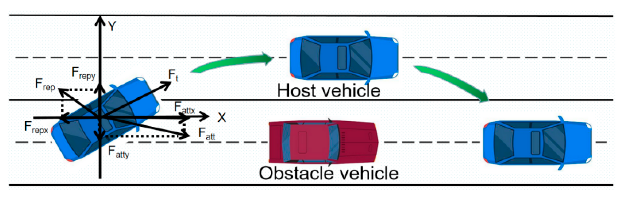
Figure 2.
APF three-dimensional potential field.
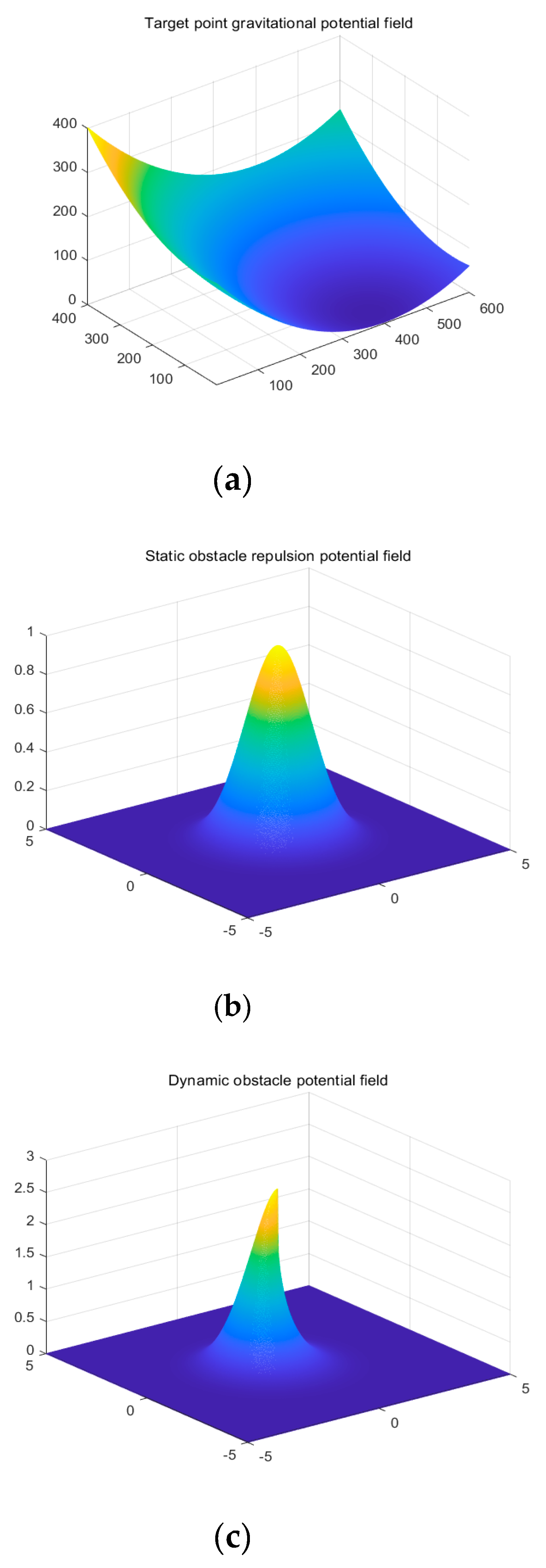
Figure 3.
Subtarget virtual potential field.
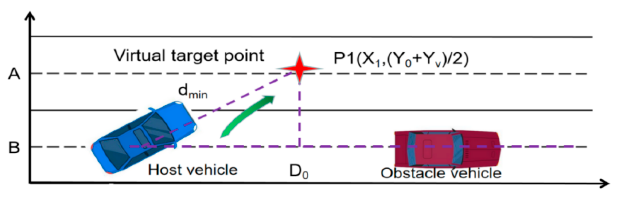
Figure 4.
Contour maps of potential fields and collision-free trajectories.
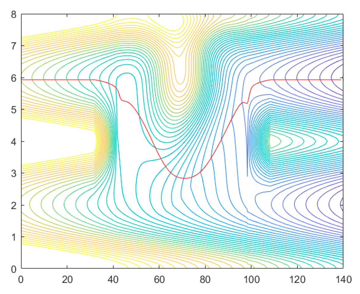
Figure 5.
Optimizing APF for overtaking and collision avoidance. (a). Change lanes with combined force; (b). Changing lanes to overtake; (c). Lane change and passing complete; (d). Return to main lane; (e). Drive smoothly to the target point.
Figure 5.
Optimizing APF for overtaking and collision avoidance. (a). Change lanes with combined force; (b). Changing lanes to overtake; (c). Lane change and passing complete; (d). Return to main lane; (e). Drive smoothly to the target point.
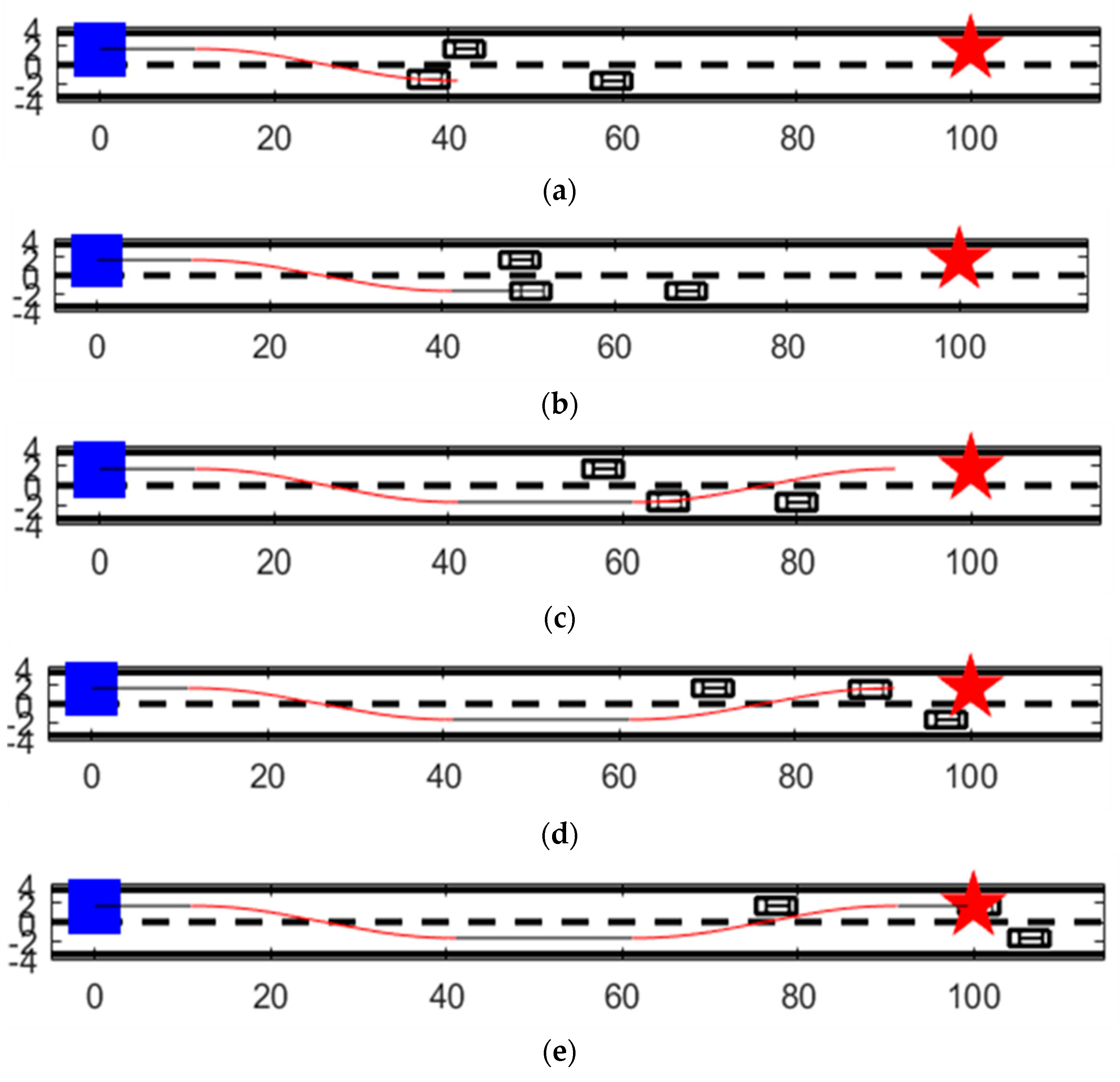
Figure 6.
Principles of vehicle dynamics.
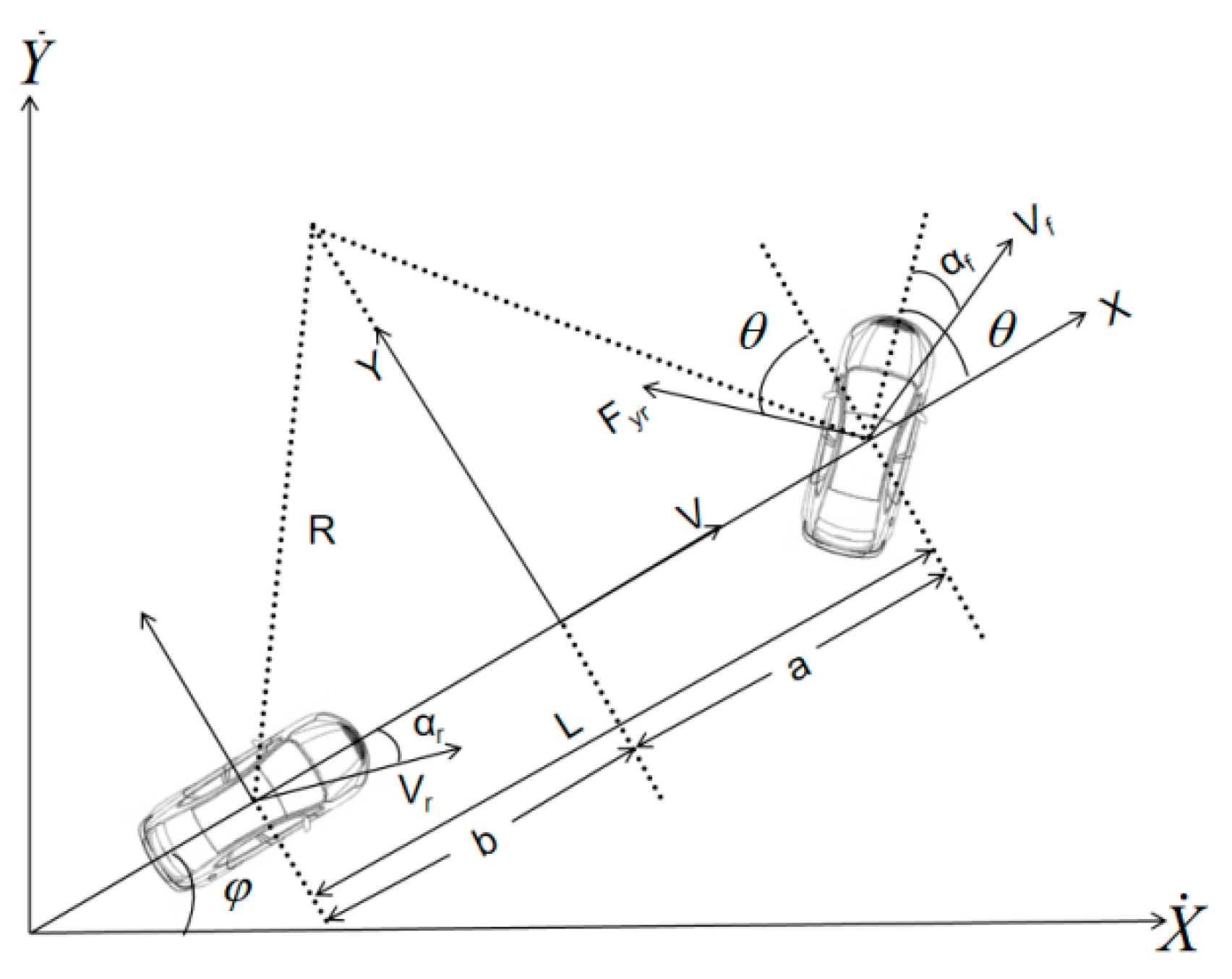
Figure 7.
Framework of DLQR tracking control algorithm.
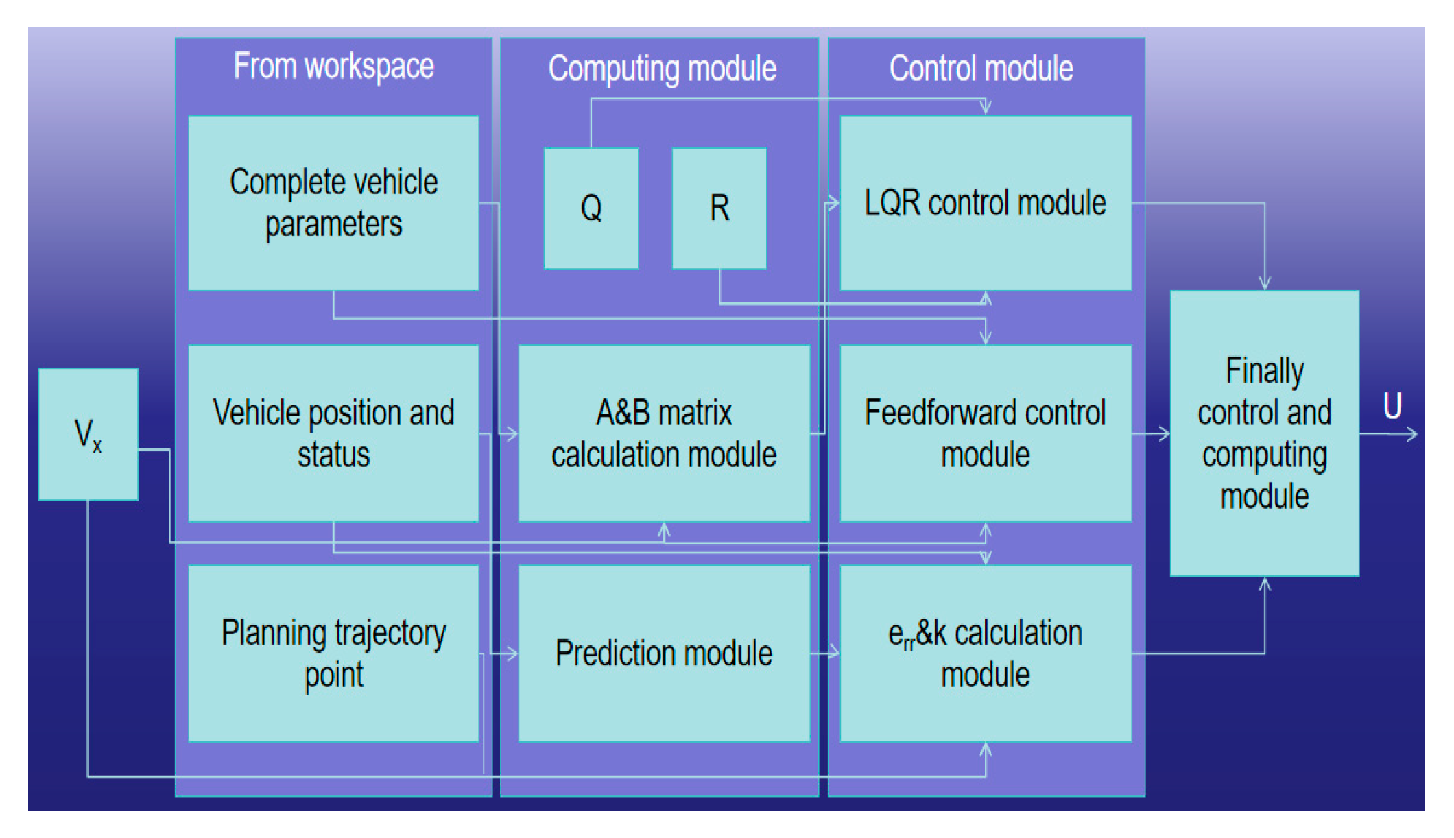
Figure 8.
Body dimensions.
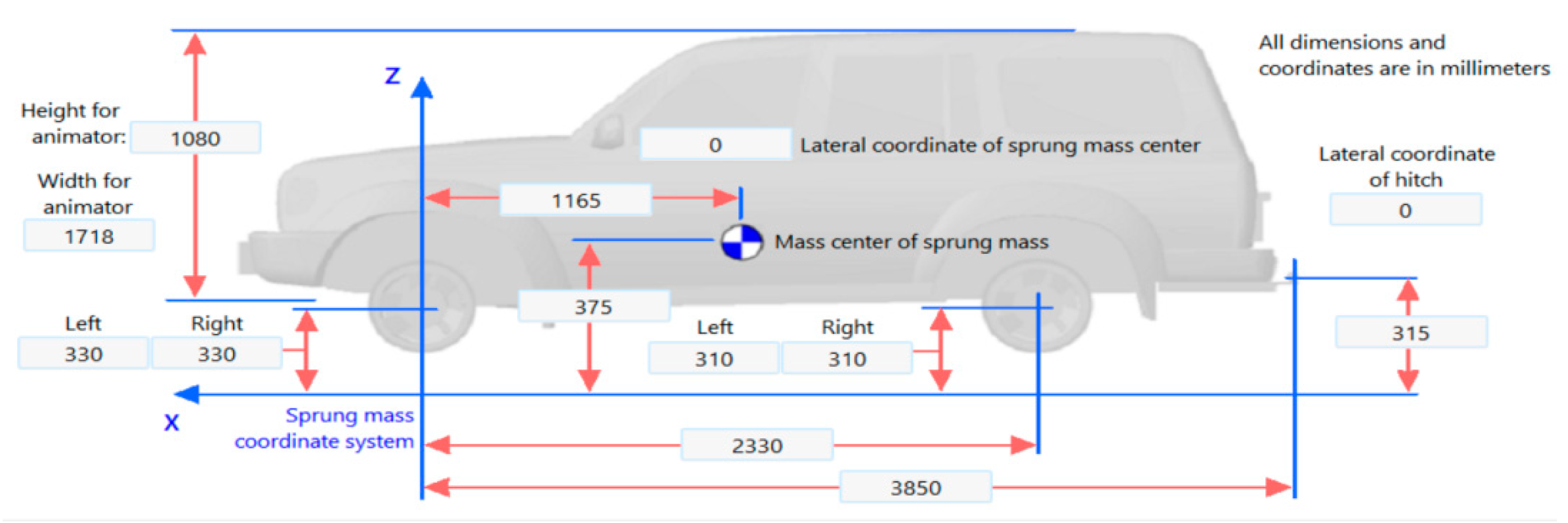
Figure 9.
CARSIM parameter configuration and simulink algorithm module co-simulation platform.
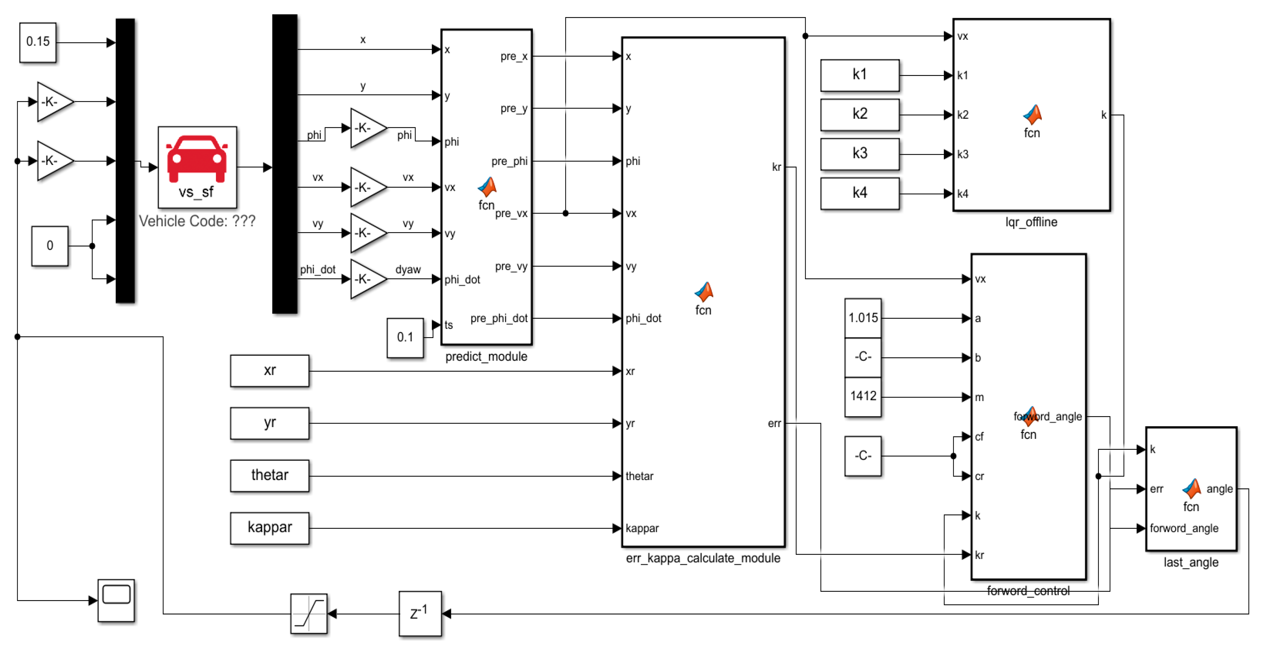
Figure 10.
Simulation analysis of obstacle avoidance in different obstacle scenarios.
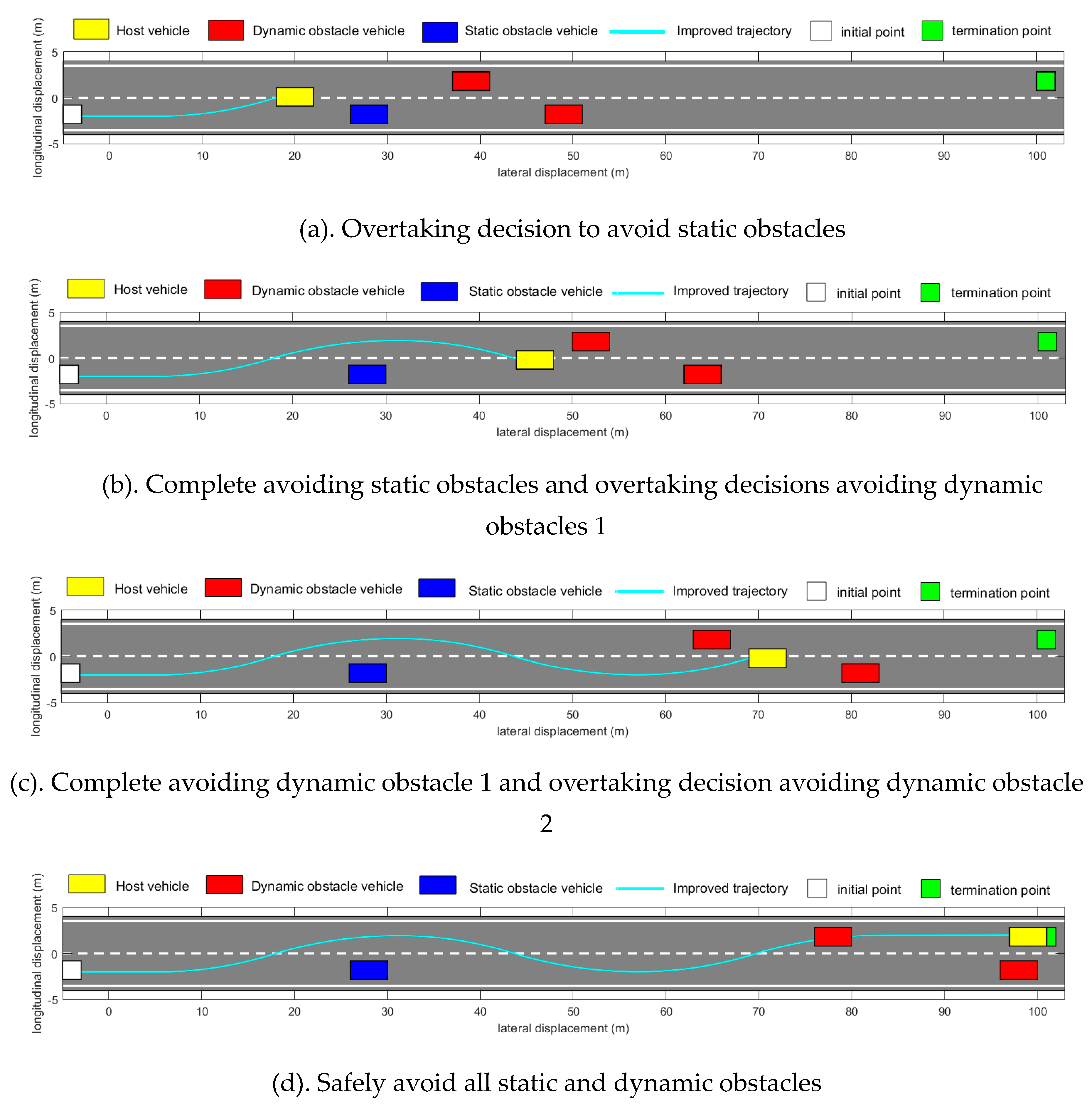
Figure 11.
Analysis of steering Angle results.
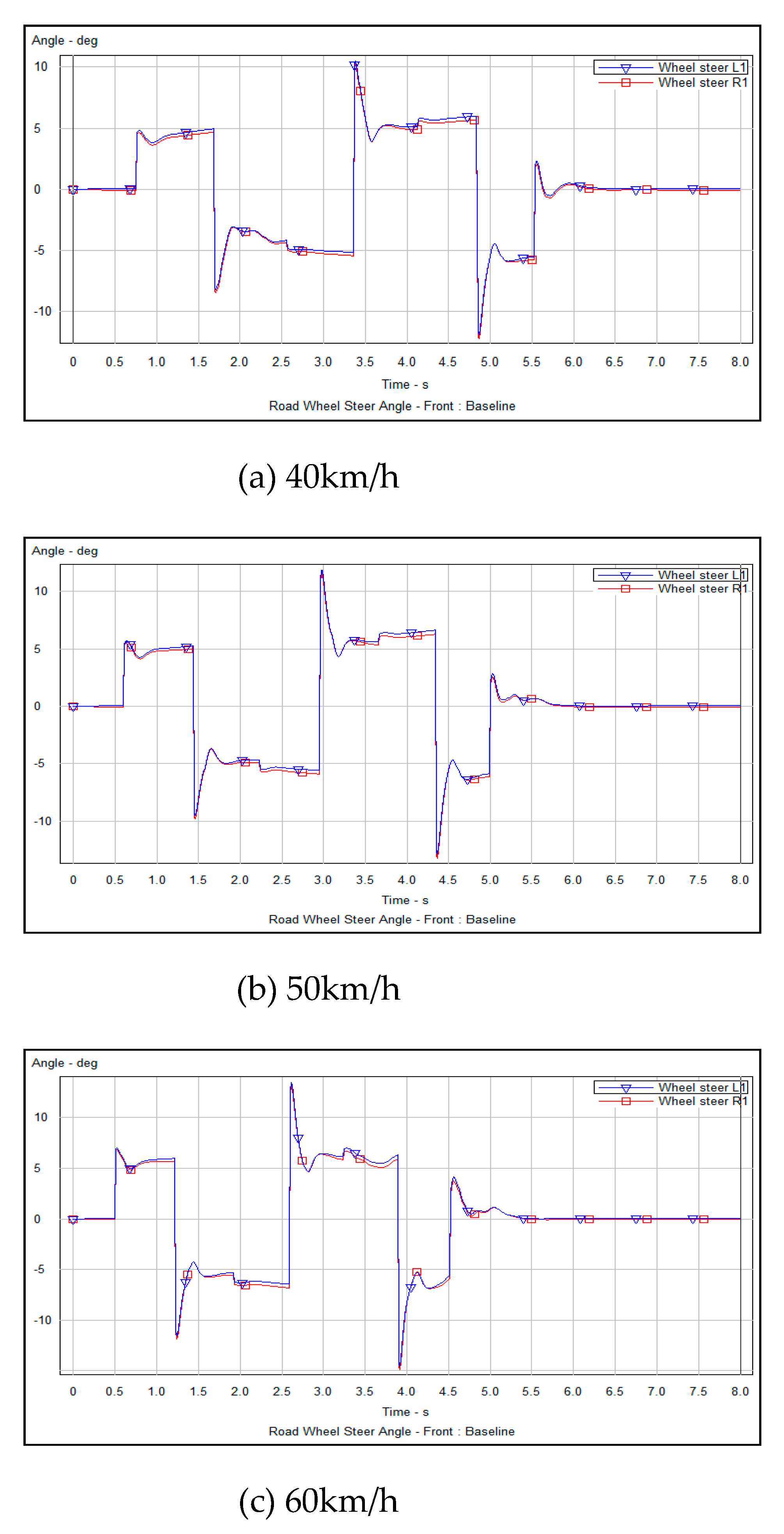
Figure 12.
Vehicle side Angle tracking motion analysis.
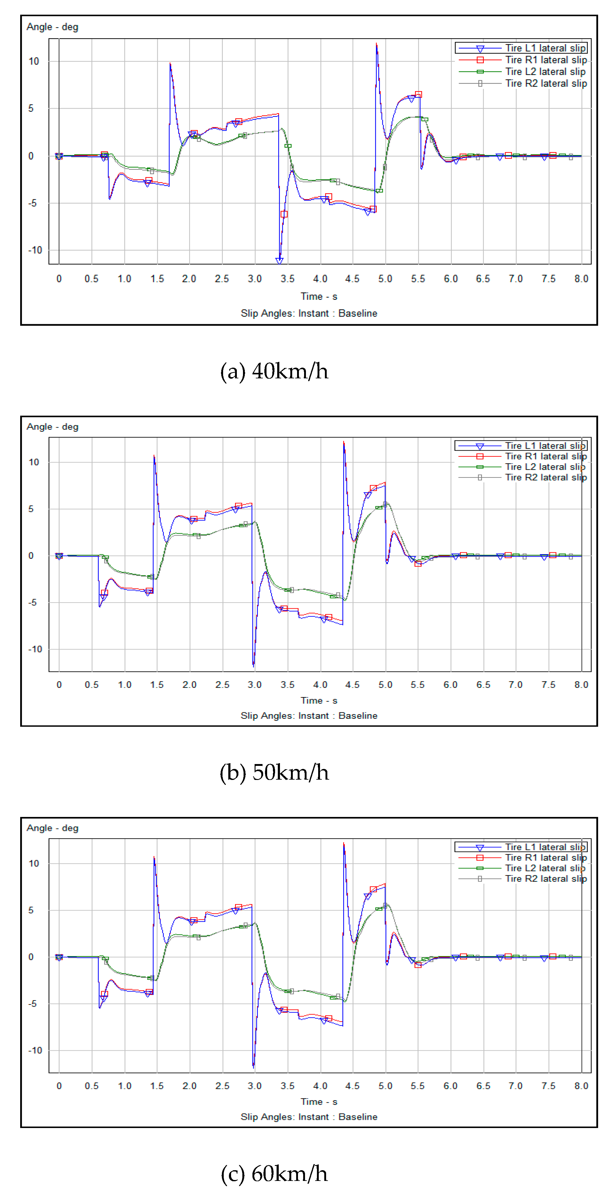
Figure 13.
Analysis of vertical support force results of vehicle tire steering.
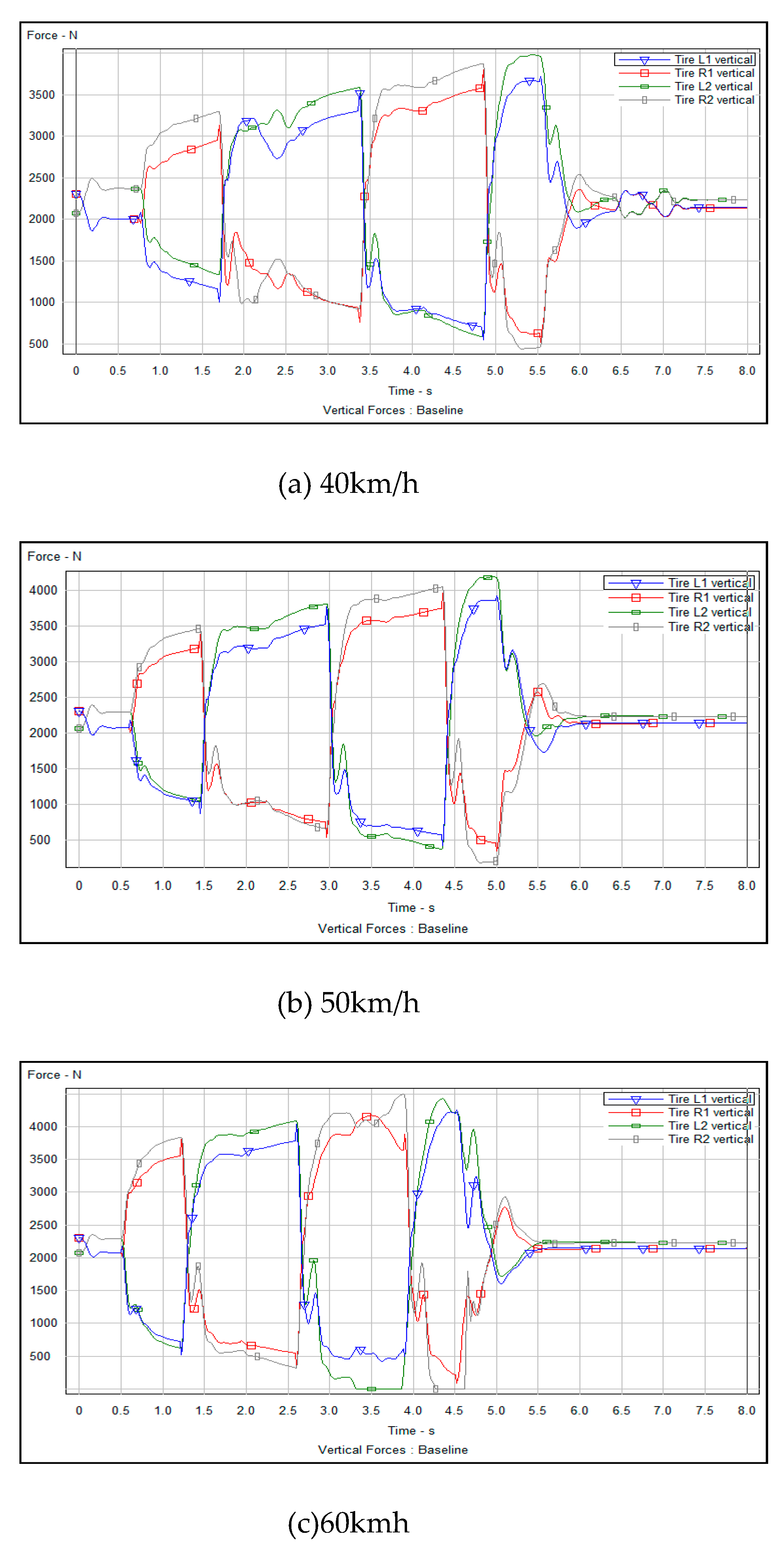

Table 1.
Vehicle parameters.
| Parameter | Value | Unit |
|---|---|---|
| Sprung mass | 1020 | kg |
| Width for animator | 1718 | mm |
| Yaw inertia | 1020 | Kg*m2 |
| Axle base | 2330 | mm |
| Height of wheel center | 310 | mm |
| Height of the center of mass | 375 | mm |
Table 2.
Comparison of simulation results of steering parameters.
| Speed (km/h) |
Maximum fluctuation range of steering Angle (deg) | Maximum fluctuation range of side deflection Angle(deg) | Maximum tire steering vertical support (N) |
|---|---|---|---|
| 40 | 4.0°- 6.0° | 0°- 6.0° | 4000 |
| 50 | 4.1°- 6.2° | 0°- 7.0° | 4250 |
| 60 | 4.3°- 6.3° | 0°- 8.0° | 4500 |
Disclaimer/Publisher’s Note: The statements, opinions and data contained in all publications are solely those of the individual author(s) and contributor(s) and not of MDPI and/or the editor(s). MDPI and/or the editor(s) disclaim responsibility for any injury to people or property resulting from any ideas, methods, instructions or products referred to in the content. |
© 2024 by the authors. Licensee MDPI, Basel, Switzerland. This article is an open access article distributed under the terms and conditions of the Creative Commons Attribution (CC BY) license (http://creativecommons.org/licenses/by/4.0/).
Copyright: This open access article is published under a Creative Commons CC BY 4.0 license, which permit the free download, distribution, and reuse, provided that the author and preprint are cited in any reuse.


