
Submitted:
04 December 2024
Posted:
05 December 2024
You are already at the latest version
Abstract
In supply chain management (SCM), the flow of goods and services from raw materials to the end user involves significant complexities and uncertainties at each stage. Computer modeling and simulation offer powerful tools to address these challenges, as they can efficiently analyze operational issues that are otherwise time-consuming and difficult to explore. Inaccurate estimation of raw materials, labor, or equipment often leads to financial losses and environmental impact, a concern for many manufacturing companies. The purpose of this study is to explore the application of system dynamics modeling (SDM) in the manufacturing of hemp-reinforced polymer composite (HRPC), with the goal of optimizing material, labor, and equipment usage. By applying system dynamics (SD), the manufacturing unit can enhance sustainability by minimizing the use of materials, labor, and equipment, thereby lowering energy consumption. For this research, the SDM software STELLA® was chosen for its affordability, ease of use, and comprehensive features, making it a strong choice compared to other leading software options. Our literature review revealed a significant gap in existing research, as we could not identify any study currently exploring the simulation of HRPC material manufacturing using SDM. Our study concludes that SDM simulation serves as an effective method for optimizing materials, labor, and equipment in the manufacturing of HRPC materials. By simulating various supply chain scenarios in a risk-free environment, the model reduces resource consumption and improves manufacturing efficiency, hence promoting sustainability. Furthermore, outputs from the STELLA® model can serve as inputs for life cycle assessment (LCA) to quantitatively evaluate environmental impacts.
Keywords:
systems dynamic modeling
; sustainable supply chain management
; hemp-reinforced polymer composite
; modeling product manufacturing
1. Introduction
Originally called industrial dynamics [1], system dynamics modeling (SDM) is a computer-aided simulation technique that provides a robust framework for framing, understanding, and discussing complex problems. SDM is based on the concept of feedback and delays [2,3]. It was developed by Professor Jay W. Forrester at the Massachusetts Institute of Technology in the mid-1950s [4].
SDM utilizes a visual programming protocol to create interactive models that simulate different scenarios by defining their scope, boundaries, and thresholds in a visual environment [5]. It has been widely applied across various sectors, including manufacturing, healthcare, and energy, to analyze and optimize complex systems by modeling feedback loops and time delays. In manufacturing, it is used to improve production efficiency and supply chain management (SCM), while in other sectors, it helps with strategic decisions such as managing resources, planning policies, and demand forecasting [6,7]
SDM in manufacturing supports sustainable practices by focusing on optimizing production processes and addressing operational challenges. It models the interactions between key factors like production rates, inventory levels, machine usage, and workforce allocation to pinpoint inefficiencies and improve overall efficiency [8,9]. Manufacturers can increase output and reduce costs by simulating various production strategies, such as changing schedules or addressing supply chain disruptions [7,10]. SDM also helps visualize feedback loops and time delays inherent in manufacturing operations [11]. For example, it can show how equipment breakdowns affect production or how changing demand affects inventory. By using these insights companies can develop strategies to minimize delays, prevent bottlenecks, and ensure smooth production. These insights can ensure smoother production processes by helping companies develop strategies to minimize delays and bottlenecks [6,10,11,12].
SCM involves managing the flow of goods and services from raw material procurement to the delivery of the final product. It focuses on enhancing efficiency and cost-effectiveness by coordinating crucial activities, including sourcing, production, logistics, and distribution [13,14]. Effective coordination of these activities is key to staying competitive. Through its holistic approach, SCM enables businesses to remain agile and responsive to market demands and challenges [15].
In recent years, sustainability has become a key consideration in supply chain management for balancing economic, environmental, and social objectives, as opposed to traditional, efficiency-driven approaches. Sustainable supply chain management (SSCM) aims to reduce environmental impact, promote social responsibility, and maintain economic viability [16]. According to Pullman and Wu adding sustainability to supply chain management involves creating processes that reduce waste, use renewable resources, and promote fair labor practices [17]. Beyond meeting regulations, these efforts focus on creating long-term value and gaining a competitive edge through innovation. These supply chains emphasize transparency, engage stakeholders, and continually improve to align with global sustainability goals and growing consumer expectations [17].
The hemp plant, cultivated for thousands of years [18] is recognized for its sustainability and versatility across various industries [18]. It requires significantly less water and pesticides than traditional crops like cotton. The hemp plant minimizes waste and promotes circular economies, as nearly every part of the plant can be utilized in diverse applications, including textiles, food products, biofuels, and construction materials [18]. Hemp-reinforced polymer composites provide many benefits in manufacturing. Polymers can be reinforced with hemp fibers due to their high specific strength and stiffness [19]. Hemp fibers are biodegradable and conform to environmental sustainability goals [18]. Composites made from hemp contribute to the development of sustainable materials, reducing the need for synthetic fibers and promoting a more sustainable manufacturing sector [20].
Creating an efficient supply chain is often challenging due to the volatility and complexities in material flow, equipment availability, and labor. To address these challenges, managers need to identify and understand the sources and impacts of these uncertainties and work to minimize or eliminate them. Current analytical tools used to assess uncertainty typically rely on traditional mathematical methods, such as single-parameter or local sensitivity analyses, which do not consider variability [21]. Simulations, on the other hand, can effectively handle variability, making it an essential tool for supply chain analysis. Companies can use computer simulations to explore operational challenges in SCM that are difficult to model and solve analytically. Simulations enable businesses to evaluate the performance and cost implications of innovative inventory systems, like just-in-time (JIT), without needing to implement them in practice [22].
To demonstrate the impact of this model on supply chain sustainability, we optimized the initial scenario and achieved a 22% increase in the availability of polymer material, a 12% reduction in the grinding rate process, and an increase of 1 decorticator (removing an equipment bottleneck). These adjustments resulted in a production rate of 9.75 tons/day of hemp-reinforced composite material, a 22% improvement over the initial rate of 8 tons/day. By addressing the lack of polymer material and adding more decorticators the optimized model increased material processing capacity and stopped the buildup of unprocessed hemp stalks from the farm. This shows how the model improves supply chain sustainability by balancing resource use and increasing efficiency.
This paper is organized as follows: Section 2 explains the rationale and objectives of the study, including a literature review on the use of SDM in SSCM. Section 3 presents the study's hypothesis and research questions. Section 4 describes the materials and methods used. Section 5 outlines the simulation results, while Section 6 provides a discussion, conclusions, and suggestions for future research.
2. Literature Review
This literature review examines SDM and its applications in manufacturing, SCM, and SSCM. It further reviews hemp-reinforced polymer composite manufacturing, with an emphasis on sustainability and the role of industrial hemp. The review concludes by identifying the research gap and presenting the study's proposed contribution.
2.1. System Dynamics Modeling and Its Applications in Manufacturing and Supply Chain Management
SDM is a valuable method for analyzing and improving complex systems in manufacturing and SCM. Forrester developed SD to model interactions, feedback loops, and delays in a system which enables a deeper understanding of how its components interact with each other within a system. SDM provides useful insights into operational inefficiencies, demand fluctuations, and process optimization [6].
In manufacturing, SD has been used to study production processes and improve resource utilization. Sterman [7] highlighted how SD models enable manufacturers to simulate the effects of production schedules, equipment downtime, and workforce allocation on overall system performance. By identifying bottlenecks and testing different strategies, companies can improve throughput and reduce costs while maintaining production stability [7].
In SCM, SD helps analyze supply chain structures and policies. Angerhofer and Angelides [2] conducted a comprehensive review, highlighting SD's role in managing demand fluctuations, inventory control, and supply chain integration. They demonstrated how SD models enable organizations to simulate and evaluate the impact of strategic decisions, such as supplier coordination and lead time reduction, on supply chain performance [2].
The integration of SD into sustainable manufacturing and SCM has also been widely explored. Rebs et al. [23] reviewed its application in designing sustainable supply chains, where SD was used to model the long-term environmental and social impacts of production and logistics decisions. These models help organizations balance economic growth with sustainability goals by identifying areas for resource efficiency and waste reduction [23].
SDM has been extensively applied in the manufacturing sector to analyze and improve complex systems [24]. In the automotive manufacturing industry, SD has been used to optimize production and inventory management. For example, Bianchi and Ferretti [25] used SD to model supply chain dynamics that improved lead times and reduced costs. This study demonstrated how SD can be used to adjust supply chain strategies as market conditions change [25].
Kibira et al. [26] developed a framework using SD to evaluate sustainable manufacturing practices. Their work focused on how manufacturing processes interact with environmental, financial, and social factors [26]. A study in 2023 examined the use of SD in manufacturing process analysis. It showed how SD can map cause-and-effect relationships and predict system behavior in different situations, while also noting its strengths and limitations [11].
Auricchio et al. developed a SD simulation model to analyze scalable-capacity manufacturing systems, emphasizing production cost efficiency and system adaptability to changes. Their research highlighted the potential of SD to optimize resource allocation and improve decision-making in dynamic manufacturing environments [27].
2.2. System Dynamics Modeling for Sustainable Supply Chain Management
SDM is a valuable tool for analyzing and improving SSCM. It helps study the complex interactions within supply chains, combining environmental, economic, and social factors to support and achieve sustainability goals [7]. Sterman emphasized that SDM is a flexible tool for understanding supply chain dynamics, including feedback loops and delays, which are crucial for studying sustainability. SDM help stakeholders test different scenarios and assess long-term impacts, supporting better decisions for sustainable practices [7].
SDM has been widely used to enhance environmental sustainability in supply chains. For example, Georgiadis and Vlachos [28] applied SDM to assess waste reduction and energy efficiency in supply chains, identifying strategies to reduce environmental impacts. Pinto and Diemer [29] used SDM to study the environmental impacts of the steel supply chain in Europe. Their research focused on finding ways to optimize resource use and reduce emissions [29].
In terms of economic benefits, Angerhofer and Angelides [2] highlighted how SDM can stabilize inventory levels, reduce costs, and improve supply chain efficiency. Similarly, Kibira et al. [26] used SDM to evaluate sustainable manufacturing practices, demonstrating how it links operational efficiency with financial and environmental performance.
SDM has also been used to address social aspects of supply chain sustainability, focusing on issues such as labor conditions, community impacts, and social equity. Rebs et al. [30] applied SDM to analyze how pressures from stakeholders, like customers and regulators, and a company’s capabilities affect the social performance of supply chains. Their study showed that improving labor conditions and supporting communities requires aligning social goals with business strategies. It highlighted the need for thoughtful decisions and policies to balance efficiency and positive social impacts.
Recent studies have used SDM to explore how new technologies impact sustainable supply chains. Khorram Niaki and Nonino [31] studied how additive manufacturing impacts supply chain dynamics and sustainability. Their study showed that SDM can effectively model technological disruptions and their effects on supply chains.
Despite its advantages, SDM has challenges. Sterman [7] noted that developing accurate models requires extensive data and expertise. Various studies have highlighted the challenge of integrating qualitative social metrics into traditionally quantitative SDM. and highlight the need for methodological approaches that effectively blend qualitative and quantitative data [32,33].
2.3. Hemp-Reinforced Polymer Composite Manufacturing for Sustainability
Sustainability has become a critical focus across industries, driven by the urgent need to minimize environmental impact, preserve resources, and address climate change. Sustainable practices strive to balance economic growth, environmental health, and social well-being to ensure the needs of the present are met without compromising future generations [34]. Sustainability in manufacturing involves minimizing waste and energy usage and using renewable resources [24,35]. Hemp is one of the natural fibers that can be used in composite manufacturing to achieve these goals [18].
Hemp is derived from the Cannabis sativa plant. It is a highly versatile crop with applications in textiles, food, construction, and composites [18]. Its sustainability arises from several factors, such as, low environmental impact [18,19], carbon sequestration [18,36], soil health [18,37] and biodegradability [18]. These attributes make hemp an attractive raw material for industries looking to enhance sustainability while maintaining performance [18].
Hemp fibers are becoming popular as a reinforcement material in polymer composites because of their strong mechanical properties [38] and environmental benefits [39]. Hemp-reinforced polymer composites are made by combining hemp fibers with a thermoplastic or thermosetting polymer matrix. These composites offer an eco-friendly alternative to traditional materials and are increasingly used in industries like automotive, construction, and packaging [19].
Although hemp-reinforced composites have many advantages, they still face challenges, such as moisture sensitivity, fiber variability, and compatibility problems with certain polymers. Research is being conducted on chemical treatments and hybrid composite designs to address these issues [40]. Materials science and manufacturing techniques offer significant opportunities for expanding their applications [39].
2.5. Identified Research Gap and the Study’s Proposed Contribution
The literature review identifies a significant research gap: the application of SDM as a sustainability decision-making tool in hemp-reinforced polymer composite (HRPC) manufacturing remains largely unexplored. While various studies have utilized SDM in the manufacturing industry, no research has specifically focused on supply chain simulation for sustainable HRPC manufacturing.
To the best of our knowledge, this study is the first to utilize SDM to simulate a supply chain for HRPC manufacturing with the goal of enhancing sustainability. Waste generation is a significant challenge in HRPC manufacturing [41]. By addressing this concern, our research highlights the potential of SDM as a decision-making tool to support sustainable practices and optimize processes in HRPC manufacturing.
3. Hypothesis and Research Questions (RQ)
Our hypothesis suggests that incorporating SDM into SSCM is as an effective strategy for optimizing materials, labor, and equipment in HRPC manufacturing. Additionally, we propose that this integration would contribute to a more sustainable manufacturing process.
RQ1: Can STELLA be applied to model HRPC manufacturing supply chains?
RQ2: Can the model simulate the HRPC supply chain?
RQ3: Can these simulations be applied to optimize material, equipment, and labor usage?
RQ4: Can the simulation output guide the development of an SSCM strategy?
4. Materials and Methods
4.1. SDM Software
There are various SDM software options available on the market, such as Powersim Studio 10, STELLA® 3.5.0, and Anylogic 8.8.4 [24]. We chose STELLA® for our study because it provides a good balance of affordability, ease of use, and functionality compared to other options.
STELLA® is a SDM software that operates using four core components: stocks, flows, converters, and connectors (Figure 1). Stocks represent the measurable quantities of a system (e.g., materials, products, currency, people) that either increase or decrease over time. Flows control the rate at which stocks grow or diminish over time by moving these measurable quantities into or out of the stocks. Converters process input data to generate an output signal, which influences the behavior of stocks and flows in the model. Connectors (illustrated as red arrows in Figure 1) transmit information between converters, stocks, and flows, enabling parameter adjustments within the model. The cloud symbol in Figure 1 defines the system boundary, setting the scope of the model. Simulations focus exclusively on changes occurring within this defined system boundary.
The steps to build a STELLA® model for SCM are as follows:
- Define the objective of the supply chain.
- Set the project scope by identifying its boundaries, inputs, and outputs.
- Specify the functional unit, such as the number of goods produced per day.
- Build the STELLA® model using the four building blocks: stocks, flows, converters, and connectors.
- Add equations with conditional statements, like "if_then_else," to the flows.
- Set initial conditions for each stock and converter.
- Run the model and observe the behavior of stocks and flows for a given scenario.
- Adjust inputs and rerun the model for different scenarios, aiming to minimize material flows and waste.
4.2. Elements of SDM
Building an SDM requires careful consideration of several key factors. The most important elements include:
- Specifying appropriate units of measurement for each model variable to avoid formulation errors.
- Ensuring model equations are unit-consistent, meaning the left and right sides of each equation must simplify to the same units.
- Maintaining consistent units of measurement across all stocks within a flow chain.
- Assigning an initial value to all stocks at time equals zero.
4.3. Supply Chain Model of Hemp-Reinforced Polymer Composite Manufacturing.
The SD model in this section simulates the supply chain and manufacturing process of up to 10 tons/day of hemp-reinforced polymer composite material produced. The number of tons of production in one day, i.e., up to10 tons/day, was chosen as an example to demonstrate the use of the model, and it does not reflect any one company's specific production. It is less important for this study to have a production number that exactly matches industry production as this number is only used to demonstrate the ability of the model to simulate and stabilize the supply chain and prove the hypothesis.
Figure 2 is the SD model using STELLA®, simulating the manufacturing process of a HRPC. This model outlines the process of producing HRPC material, beginning with the transportation of raw hemp from a farm to a factory. At the factory, the hemp is decorticated to separate it into greens, fiber, and hurd. Hemp hurd is the woody core of the hemp stem, also known as shive. It has many potential industrial applications including building materials, insulation, fluid absorbing materials, and composite reinforcement. The separated greens and fiber are sent to their respective processing units, while polymer powder (or pellets) is transported to the factory to be blended with the hurd. The hurd is ground and mixed with the polymer powder in specific proportions based on the reinforced fraction. This mixture is then compounded to create the HRPC material, which is subsequently transported to a post-processing facility for further processing.
Since hurd is the lowest-value material of the hemp plant, researchers are investigating methods to process it into higher-value products. One promising application involves grinding hurd into short pieces and combining it with a polymer to create composite materials. As this application is still under research, it has been chosen as the focus of this study.
Figure 2 was developed using proprietary information obtained from various industry sources and hemp processing companies that prefer to remain anonymous and is based on the following assumptions. -
- Harvested and retted hemp stalks are delivered to the manufacturing facility to begin the production process. It is assumed that farms can consistently supply the facility with sufficient material. Any processes prior to delivering harvested and retted hemp stalks are outside the scope of this model.
- Hemp stalks are processed through decortication, separating them into three components: bast fiber, hurd, and greens.
- "Greens" refer to any residues and leaves separated during decortication that are neither bast fiber nor hurd.
- Bast fiber and greens are transported to their respective manufacturing facilities.
- Each step of the process generates a nominal amount of waste.
- Thermoplastic polymer powder or pellets are purchased from suppliers and delivered to the manufacturing facility.
- The reinforcement fraction for the composite material is specified by an external customer purchasing the material.
- The composite material is processed into compounded pellets, which are then transported to customers for further processing. The conversion of pellets into final products is beyond the scope of this model.
- The current model does not account for supply chain disruptions such as equipment failures, transportation delays, or labor shortages (though these time-dependent elements could be added in future versions of the model).
These assumptions provide the foundation for Figure 2, illustrating the manufacturing and supply chain processes of hemp-reinforced polymer composite materials.
4.4. Development of SDM Converters, Flow Equations, and Stock Equations for This Model
The next step in this model involves generating equations for all flows, stocks, and the initial values of the converters. This process must be carried out for each flow, converter, and stock within the model. Figure 3 provides an example by isolating the specific stock, Whole Stalk, and illustrating its associated flows and converters, offering a clear view of how the components interact within the system.
4.4.1. SDM Converters in Figure 3
In the Hemp Transport from Farm flow depicted in Figure 3, the transport process facilitates the movement of hemp from the farm to the factory. The quantity transported is determined by the supply from the hemp farm, which is entered as an input value in the corresponding converter. Similarly, in the Decortication flow, decorticators are employed to separate whole stalks into greens, hurd, and fiber. The input values for The Number of Decorticators and the Maximum Whole Stock Quantity that Decorticators can Process per day are entered into their respective converters to facilitate accurate modeling and simulation of the processing capacity. The converters utilized in Figure 3 are detailed in Table 4.
4.4.2. SDM Flow Equations in Figure 3
Note that the flow equation in Table 5 uses an "if_then_else" statement. In Table 5, in Decortication (flow #2).To understand this equation, consider the following numerical example. If the input value of converter Maximum Whole Stalk Quantity that the Decorticator can Process is 80 tons/day and there are 2 decorticators, the maximum Decortication flow would be 160 tons/day. However, if the Whole Stalk stock is only 50 tons/day, the maximum Decortication flow would be limited to 50 tons/day and not reach the maximum of 160 tons/day. Conversely, if the Whole Stalk stock is 200 tons, the Decortication flow would still be capped at the maximum rate of 160 tons/day, leaving 40 tons of Whole Stalk stock unprocessed.
4.4.3. SDM Stock Equation in Figure 3
Stock equations are mass balances of the flows in and out of the stock (Equation (1)).
dt = the time step in the model run (here, 1 day) (1 day is the time step of the simulation, so calculations are made once per day).
Stock (t) = Stock (t − dt) + ∑ Inflows − ∑ Outflows
t = a particular time point in the model run (here, 1–20 days) (It was observed that the simulation reached equilibrium within 20 days).
Specifically, in Table 6 below, the inflow is Hemp Transport from Farm, and the outflow is Whole Stalk.
Following this procedure, the remaining flows, stocks, and converters are developed and described in detail in Appendix A in Table A1, Table A2 and Table A3. These tables provide comprehensive information for the reader's convenience, ensuring clarity and ease of reference for all components of the model.
This section demonstrates that STELLA® can be applied to model the manufacturing supply chain for HRPC materials. This addresses Research Question 1, Can STELLA® be applied to model HRPC manufacturing supply chains?
5. Simulation Results
5.1. Initial Simulation
Figure 4 below shows the initial simulation using this model. The converter values for this simulation are listed in Table 7. These values, or input numbers, represent typical averages derived from proprietary information provided by various hemp processing companies, which remain unidentified in this study. The definitions for all stocks, converters, and flows are provided in Section 4.3, in Table 1, Table 2 and Table 3, respectively.
The final result values for all stocks and flows from the initial simulation, spanning days 1 to 20, are presented in Table A4 and Table A5 in Appendix B. The appendix contains detailed tables for the reader's convenience.
According to Table A4 (Flows), the initial simulation using the converter/input values from Table 7 fails to achieve the target production of 10 tons of HRPC material per day (Transport to Post Processing) and instead produces only 8 tons per day.
Similarly, Table A5 (Stocks) shows that the stock values fluctuate over time and do not stabilize to an equilibrium. For instance, the stocks of Inhouse Ground Hurd and Whole Stalk exhibit opposing trends—Inhouse Ground Hurd decreases while Whole Stalk increases over time, reflecting imbalances in the supply chain. Specifically:
- Inhouse Ground Hurd stock declines, with values dropping from 1.66 tons on day 6 to 1.34 tons on day 10, and further to 0.552 tons on day 20.
- Whole Stalk stock rises, increasing from 3.2 tons on day 6 to 4.96 tons on day 10, and reaching 9.36 tons by day 20.
These trends indicate the presence of choke points in the supply chain, where resource limitations hinder material processing at an adequate rate. This results in material accumulation before the choke points and depletion after them, disrupting the flow and balance of the supply chain.
To stabilize the supply chain simulation, the next step involves systematically adjusting the converter values to eliminate resource limitations. These modifications aim to ensure that material is processed at a sufficient rate, ultimately achieving the target production of 10 tons per day of hemp-reinforced composite material.
Although these converter values do not optimize or stabilize the supply chains, they successfully demonstrate that the model can simulate the hemp-reinforced polymer composite (HRPC) manufacturing process. This addresses Research Question 2: Can the model simulate the HRPC supply chain?
5.2. Stabilized Supply Chain Simulation
Figure 5 illustrates a stabilized supply chain simulation achieved using the algorithm developed in this study to adjust converter values. The details of the algorithm are provided later in this section. The adjusted converter values for this simulation are listed in Table 8.
Stabilizing the model required multiple iterations to achieve a balanced and stable outcome. On average, 10–20 iterations were performed for each stock, adjusting the converter values to identify optimal settings for stability. With 9 stocks in the model, this process involved approximately 90–180 iterations in total. The primary challenge was determining the appropriate converter values to maintain stability without introducing oscillations or instability in the stocks. This demanded careful adjustments and thorough testing of both stocks and converter values to ensure the model's dynamics were effectively controlled.
Table A6 (Flows) and Table A7 (Stocks) in Appendix C present the final result values for all stocks and flows from the stabilized supply chain simulation over 1 to 20 days. The appendix contains detailed tables for the reader's convenience.
According to Table A6, the supply chain simulation using the converter/input values from Table 8 closely approaches the goal of producing up to 10 tons/day of hemp-reinforced composite material (Transport to Post Processing).
As shown in Table A6, the simulation achieves a stable supply chain since the stocks reach equilibrium values without fluctuating over time, indicating no depletion or buildup of hemp material. For instance:
- The stock of Inhouse Ground Hurd stabilizes at 1.69 tons/day after 6 days.
- The stock of Whole Stalk also stabilizes at 1.32 tons/day and no longer increases over time.
All stocks now remain constant, indicating no material buildup or depletion in the supply chain. This reflects the absence of resource limitations and ensures that material is processed efficiently. Unlike the initial simulation described in Section 4.1, this stabilized simulation eliminates choke points, allowing for an uninterrupted flow of materials through the supply chain.
The following algorithm was used to determine the converter values that produce a stabilized supply chain, as shown in Table 8:
- Evaluate the Final Stock:
Start with the last stock in the supply chain. Check if its value changes over time.
- If the value does not change with time, move to the next upstream stock in the supply chain.
- If the value does change with time, proceed to step 2.
- 2.
- Adjust Input Flow Converters:
Modify the converters influencing the input flow to that stock. Re-run the simulation to check if the stock value still changes with time.
- If the value continues to change, proceed to step 3.
- If the value remains unchanged, go to step 4.
- 3.
- Repeat Adjustments:
Continue adjusting the relevant converters and re-running the simulation until the stock value remains stable over time.
- 4.
- Move Upstream:
Once the current stock is stabilized, move to the next upstream stock in the supply chain. Repeat steps 1 through 3 for each stock until the first stock at the start of the supply chain is reached.
This iterative process ensures all stocks achieve stability, resulting in a fully stabilized supply chain simulation.
5.3. Analysis of Stable Supply Chain
By applying the algorithm described above, three specific converters—Grinding Rate, Number of Decorticators, and Polymer Transport Rate—were identified and adjusted, as shown in Table 9. These converters serve as examples to illustrate the stabilization process and to achieve the target production rate of up to 10 tons/day of hemp-reinforced composite material.
As detailed in Table 9, the initial converter values (3rd column) were adjusted (4th column) to achieve a stable supply chain simulation. The adjustments resulted in:
- A 22% increase in the availability of polymer (material).
- A 12% reduction in the grinding rate (process).
- An increase of 1 decorticator (equipment).
These changes led to a production rate of 9.75 tons/day of hemp-reinforced composite material, representing a 22% improvement over the initial rate of 8 tons/day. In the initial simulation, the composite material production was constrained by insufficient polymer material. By increasing the polymer supply and the number of decorticators, more composite material could be processed, preventing the buildup of unprocessed hemp stalks transported from the farm.
The algorithm outlined in this section successfully adjusted converter values to stabilize the use of materials and equipment, leading to a balanced and stable supply chain. This validates the hypothesis that SDM can effectively simulate the industrial hemp supply chain and support decision-making for efficient equipment and material utilization.
The proposed algorithm calibrates converter values to optimize the use of materials, labor, and equipment, thereby creating a more sustainable supply chain. This addresses Research Question 3: Can these simulations be applied to optimize material, equipment, and labor usage?
6. Conclusions, Limitations, and Future Work
This study demonstrates that SDM can be used to stabilize material flow in supply chain simulations while helping manufacturers identify areas of resource efficiency and improve supply chain stability. By simulating various manufacturing scenarios in a risk-free environment, the model provides a practical tool for making informed business decisions and mitigating risks when starting or investing in hemp industrial product companies. Additionally, the validated model can be customized using proprietary supply chain data making it transferable and applicable for companies planning to manufacture hemp-reinforced polymer composite materials in the future.
As discussed in Section 5.2, material flow stabilization can be achieved based on production units, enabling efficient resource utilization. Figure 5 illustrates the stabilized scenario for the model, where up to 10 tons/day of hemp-reinforced composite material is produced. In this scenario, material and equipment usage is stable, resulting in a more efficient manufacturing process.
In contrast, Section 5.1 describes an unbalanced and unstable scenario, as shown in Figure 4, where the supply chain remains unstable due to limitations in the Polymer Transport Rate, Grinding Rate, and an insufficient Number of Decorticators. These constraints lead to inefficient resource use in the manufacturing process. Table 9 highlights the adjustments necessary for achieving a balanced and sustainable supply chain.
SDM enables management to address the complexities and uncertainties inherent in SCM, as discussed in Section 1 and Section 2. By running multiple simulations, SDM allows decision-makers to identify bottlenecks, vulnerabilities, and leverage points. These are the key areas where small adjustments can significantly improve system performance, such as the Ground Hurd in this model.
Organizations can also improve decision-making and efficiency through supply chain modeling, which helps reduce materials and equipment usage. These models can assess the effectiveness and cost-efficiency of new inventory systems, such as just-in-time (JIT) [22]. JIT streamlines operations by aligning raw-material orders directly with production schedules through close coordination with suppliers.
Despite its many advantages SDM has seen limited adoption in the hemp material manufacturing supply chain as discussed in Section 2 and Section 3. This is due to several factors, including the complexity of creating and maintaining SDM models, the requirement for specialized skills, and a lack of awareness about its potential benefits. Additionally, the model presented in this study represents a stable equilibrium solution for a specific set of inputs and does not account for factors such as demand amplification, supply chain delays, or disruptions. These limitations highlight the need for further research to expand the model's applicability and robustness.
This study serves as a foundation for more detailed qualitative research on environmental sustainability, such as life cycle assessments (LCA). Future models can address current limitations by converting constant converters into time-dependent functions and incorporating feedback loops to address challenges such as inventory management and demand fluctuations. By addressing these areas, future research can build on the insights presented in this study to advance the use of SDM in sustainable supply chain management and HRPC manufacturing.
This analysis provides decision-makers with material flow input that can be used to improve the assessment of key factors such as energy consumption, greenhouse gas emissions, solid waste, and other elements that shape LCA sustainability strategies. This addresses Research Question 4: Can the simulation output guide the development of a SSCM strategy?
Author Contributions
Conceptualization, Gurinder Kaur and Ronald Kander; methodology, Gurinder Kaur and Ronald Kander; writing—original draft preparation, Gurinder Kaur; writing—review and editing, Gurinder Kaur and Ronald Kander; visualization, Gurinder Kaur; supervision, Ronald Kander; project administration, Gurinder Kaur; funding acquisition, Ronald Kander. All authors have read and agreed to the published version of the manuscript.
Funding
This research received no external funding.
Conflicts of Interest
The authors declare no conflict of interest.
Appendix A

Table A1.
Flows and flow equations in Figure 3.
Table A1.
Flows and flow equations in Figure 3.
|
Serial Nos. |
Name of the Flow | Equations | Unit |
| 1 | Compounding | IF ("Ground_Hurd_+_Polymer_Powder"/DT) < Maximum_Compounding_Rate THEN "Ground_Hurd_+_Polymer_Powder"/DT ELSE Maximum_Compounding_Rate | Tons/day |
| 2 | Compounding Waste | Compounding * Compounding_Waste_Fraction | Tons/day |
| 3 | Decortication | IF((Whole_Stalk/DT)<Maximum_whole_stalk_quantity_that_decorticator_can_process *Number_of_Decorticator) THEN (Whole_Stalk/DT) ELSE (Maximum_whole_stalk_quantity_that_decorticator_can_process * Number_of_Decorticator) | Tons/day |
| 4 | Decorticator Waste | (Fiber_Seperation+Green_Seperation+Hurd_Seperation)*Decortication_Waste_Fraction | Tons/day |
| 5 | Fiber Separation | Separated_Stalks/DT * Fiber_Fraction | Tons/day |
| 6 | Green Separation | Separated_Stalks/DT * Green_Fraction | Tons/day |
| 7 | Grinder Waste | Hurd_Grinding * Grinder_Waste_Fraction | Tons/day |
| 8 | Hemp Transport from Farm | Hemp_Transfer_from_Farm | Tons/day |
| 9 | Hurd Grinding | IF (Inhouse_Hurd/DT<Grinding_Rate) THEN Inhouse_Hurd/DT ELSE Grinding_Rate | Tons/day |
| 10 | Hurd Separation | Hurd_Fraction * Separated_Stalks/DT | Tons/day |
| 11 | Transfer of Hurd into Blender | IF ((Inhouse_Ground_Hurd/(Inhouse_Ground_Hurd+Polymer_Powder)>Hemp's_Reinforcement_Fraction_for_3D_Printed_Final_Product) THEN (Polymer_Powder/DT)*Hemp's_Reinforcement_Fraction_for_3D_Printed_Final_Product/(1-Hemp's_Reinforcement_Fraction_for_3D_Printed_Final_Product) ELSE Inhouse_Ground_Hurd/DT | Tons/day |
| 12 | Transfer of Polymer into Blender | IF ((Inhouse_Ground_Hurd/(Inhouse_Ground_Hurd+Polymer_Powder)>Hemp's_Reinforcement_Fraction_for_3D_Printed_Final_Product) THEN Polymer_Powder/DT ELSE ((Inhouse_Ground_Hurd/DT)*(1-Hemp's_Reinforcement_Fraction_for_3D_Printed_Final_Product)/Hemp's_Reinforcement_Fraction_for_3D_Printed_Final_Product) | Tons/day |
| 13 | Transport from Polymer Supplier | Polymer_Transport_Rate | Tons/day |
| 14 | Transport to Fiber Processor | IF ((Fiber/DT) < Maximum_Transport_Rate_for_Fibers) THEN Fiber/DT ELSE Maximum_Transport_Rate_for_Fibers | Tons/day |
| 15 | Transport to Greens Processor | IF ((Greens/DT) < Maximum_Transport_Rate_for_Greens) THEN Greens/DT ELSE Maximum_Transport_Rate_for_Greens | Tons/day |
| 16 | Transport to post-processing | IF Composite_material/DT < Transport_Rate THEN Composite_material/DT ELSE Transport_Rate | Tons/day |
Table A2.
Stocks and stock equations in Figure 3.
Table A2.
Stocks and stock equations in Figure 3.
|
Serial Nos. |
Stocks (all numbers are per day) |
Stock’s Variable Name |
Equation of Stock | Unit |
| 1 | Composite Material | Composite_Material | Composite Material (t-dt) + Compounding (t) - Compounding Waste (t) - Transport Rate (t) | Tons |
| 2 | Fiber | Fiber | Fiber (t-dt) + Fiber Separation (t) - Transport to Fiber Processor (t) | Tons |
| 3 | Greens | Greens | Greens (t-dt) + Green Separation (t) - Transport to Greens Processor (t) | Tons |
| 4 | Ground Hurd + Polymer Powder | Ground_Hurd_+_ Polymer_Powder |
Ground Hurd + Polymer Powder (t-dt) + Transfer of Hurd into Blender (t) + Transfer of Polymer into Blender (t) - Compounding (t) | Tons |
| 5 | Inhouse Ground Hurd | Inhouse_Ground_Hurd | Inhouse Ground Hurd (t-dt) + Hurd Grinding (t) - Grinding Waste (t) - Transfer of Hurd into Blender (t) | Tons |
| 6 | Inhouse Hurd | Inhouse_Hurd | Inhouse Hurd (t-dt) + Hurd Separation (t) - Hurd Grinding (t) | Tons |
| 7 | Polymer Powder | Polymer_Powder | Polymer Powder (t-dt) + Transport from Polymer Supplier (t) - Transfer of Polymer into Blender (t) | Tons |
| 8 | Separated Stalks | Separated_Stalks | Separated Stalks (t-dt) + Decortication (t) - Fiber Separation (t) - Green Separation (t) - Hurd Separation (t) | Tons |
| 9 | Whole Stalk | Whole_Stalk | Whole Stalk (t-dt) + Hemp Transport from Farm (t) – Decortication (t) | Tons |
Table A3.
Converters in Figure 3.
Table A3.
Converters in Figure 3.
|
Serial Nos. |
Converters | Converter’s Variable Name | Unit |
| 1 | Compounding Waste Fraction | Compounding_Waste_Fraction | Unitless |
| 2 | Decortication Waste Fraction | Decortication_Waste_Fraction | Unitless |
| 3 | Fiber Fraction | Fiber_Fraction | Unitless |
| 4 | Green Fraction | Green_Fraction | Unitless |
| 5 | Grinder Waste Fraction | Grinder_Waste_Fraction | Unitless |
| 6 | Grinding Rate | Grinding_Rate | Tons/day |
| 7 | Hemp Transfer from Farm | Hemp_Transfer_from_Farm | Tons/day |
| 8 | Hemp's Reinforcement Fraction for 3D Printed Final Product |
Hemp's_Reinforcement_Fraction_for_3D_Printed_Final_Product | Unitless |
| 9 | Hurd Fraction | Hurd_Fraction | Unitless |
| 10 | Maximum Compounding Rate | Maximum_Compounding_Rate | Tons/day |
| 11 | Maximum Transport Rate for Fibers | Maximum_Transport_Rate_for_Fibers | Tons/day |
| 12 | Maximum Transport Rate for Greens | Maximum_Transport_Rate_for_Greens | Tons/day |
| 13 | Maximum Whole Stalk Quantity that Decorticator can Process |
Maximum_Whole_Stalk_Quantity_that_Decorticator_can_Process | Tons/day |
| 14 | Number of Decorticators | Number_of_Decorticators | Unitless |
| 15 | Polymer Transport Rate | Polymer_Transport_Rate | Tons/day |
| 16 | Transport Rate | Transport_Rate | Tons/day |
Appendix B
Table A4.
Flow results for initial simulation (1).
| Serial Nos. | Compounding | Compounding Waste | Decortication | Decorticator Waste | Fiber Separation | Green Separation | Grinder Waste | Hemp Transport from Farm |
| 1 | 1 | 0.05 | 0.88 | 0.1 | 0.5 | 0.05 | 0.05 | 1.32 |
| 2 | 1.05 | 0.0526 | 0.88 | 0.078 | 0.39 | 0.039 | 0.0225 | 1.32 |
| 3 | 8.42 | 0.421 | 0.88 | 0.0802 | 0.401 | 0.0401 | 0.0176 | 1.32 |
| 4 | 8.42 | 0.421 | 0.88 | 0.08 | 0.4 | 0.4 | 0.018 | 1.32 |
| 5 | 8.42 | 0.421 | 0.88 | 0.08 | 0.4 | 0.4 | 0.018 | 1.32 |
| 6 | 8.42 | 0.421 | 0.88 | 0.08 | 0.4 | 0.4 | 0.018 | 1.32 |
| 7 | 8.42 | 0.421 | 0.88 | 0.08 | 0.4 | 0.4 | 0.018 | 1.32 |
| 8 | 8.42 | 0.421 | 0.88 | 0.08 | 0.4 | 0.4 | 0.018 | 1.32 |
| 9 | 8.42 | 0.421 | 0.88 | 0.08 | 0.4 | 0.4 | 0.018 | 1.32 |
| 10 | 8.42 | 0.421 | 0.88 | 0.08 | 0.4 | 0.4 | 0.018 | 1.32 |
| 11 | 8.42 | 0.421 | 0.88 | 0.08 | 0.4 | 0.4 | 0.018 | 1.32 |
| 12 | 8.42 | 0.421 | 0.88 | 0.08 | 0.4 | 0.4 | 0.018 | 1.32 |
| 13 | 8.42 | 0.421 | 0.88 | 0.08 | 0.4 | 0.4 | 0.018 | 1.32 |
| 14 | 8.42 | 0.421 | 0.88 | 0.08 | 0.4 | 0.4 | 0.018 | 1.32 |
| 15 | 8.42 | 0.421 | 0.88 | 0.08 | 0.4 | 0.4 | 0.018 | 1.32 |
| 16 | 8.42 | 0.421 | 0.88 | 0.08 | 0.4 | 0.4 | 0.018 | 1.32 |
| 17 | 8.42 | 0.421 | 0.88 | 0.08 | 0.4 | 0.4 | 0.018 | 1.32 |
| 18 | 8.42 | 0.421 | 0.88 | 0.08 | 0.4 | 0.4 | 0.018 | 1.32 |
| 19 | 8.42 | 0.421 | 0.88 | 0.08 | 0.4 | 0.4 | 0.018 | 1.32 |
| 20 | 8.42 | 0.421 | 0.88 | 0.08 | 0.4 | 0.4 | 0.018 | 1.32 |
Table A4.
Flow results for initial simulation (2).
|
Serial Nos. |
Hurd Grinding | Hurd Separation | Transfer of Hurd into Blender | Transfer of Polymer into Blender | Transport from Polymer Supplier | Transport to Fiber Processor | Transport to Greens Processor | Transport to post-processing |
| 1 | 1 | 0.45 | 0.0526 | 1 | 8 | 1 | 1 | 1 |
| 2 | 0.45 | 0.351 | 0.421 | 8 | 8 | 0.5 | 0.05 | 0.95 |
| 3 | 0.351 | 0.361 | 0.421 | 8 | 8 | 0.39 | 0.039 | 1 |
| 4 | 0.361 | 0.36 | 0.421 | 8 | 8 | 0.401 | 0.0401 | 8 |
| 5 | 0.36 | 0.36 | 0.421 | 8 | 8 | 0.4 | 0.04 | 8 |
| 6 | 0.36 | 0.36 | 0.421 | 8 | 8 | 0.4 | 0.04 | 8 |
| 7 | 0.36 | 0.36 | 0.421 | 8 | 8 | 0.4 | 0.04 | 8 |
| 8 | 0.36 | 0.36 | 0.421 | 8 | 8 | 0.4 | 0.04 | 8 |
| 9 | 0.36 | 0.36 | 0.421 | 8 | 8 | 0.4 | 0.04 | 8 |
| 10 | 0.36 | 0.36 | 0.421 | 8 | 8 | 0.4 | 0.04 | 8 |
| 11 | 0.36 | 0.36 | 0.421 | 8 | 8 | 0.4 | 0.04 | 8 |
| 12 | 0.36 | 0.36 | 0.421 | 8 | 8 | 0.4 | 0.04 | 8 |
| 13 | 0.36 | 0.36 | 0.421 | 8 | 8 | 0.4 | 0.04 | 8 |
| 14 | 0.36 | 0.36 | 0.421 | 8 | 8 | 0.4 | 0.04 | 8 |
| 15 | 0.36 | 0.36 | 0.421 | 8 | 8 | 0.4 | 0.04 | 8 |
| 16 | 0.36 | 0.36 | 0.421 | 8 | 8 | 0.4 | 0.04 | 8 |
| 17 | 0.36 | 0.36 | 0.421 | 8 | 8 | 0.4 | 0.04 | 8 |
| 18 | 0.36 | 0.36 | 0.421 | 8 | 8 | 0.4 | 0.04 | 8 |
| 19 | 0.36 | 0.36 | 0.421 | 8 | 8 | 0.4 | 0.04 | 8 |
| 20 | 0.36 | 0.36 | 0.421 | 8 | 8 | 0.4 | 0.04 | 8 |
Table A5.
Stock results for initial simulation.
|
Serial Nos. |
Composite material | Fiber | Greens | Ground Hurd + Polymer Powder | Inhouse Ground Hurd | Inhouse Hurd | Polymer Powder | Separated Stalks | Whole Stalk |
| 1 | 1 | 1 | 1 | 1 | 1 | 1 | 1 | 1 | 1 |
| 2 | 0.95 | 0.5 | 0.05 | 1.05 | 1.9 | 0.45 | 8 | 0.78 | 1.44 |
| 3 | 1 | 0.39 | 0.039 | 8.42 | 1.9 | 0.351 | 8 | 0.802 | 1.88 |
| 4 | 8 | 0.401 | 0.0401 | 8.42 | 1.82 | 0.361 | 8 | 0.8 | 2.32 |
| 5 | 8 | 0.4 | 0.4 | 8.42 | 1.74 | 0.36 | 8 | 0.8 | 2.76 |
| 6 | 8 | 0.4 | 0.4 | 8.42 | 1.66 | 0.36 | 8 | 0.8 | 3.2 |
| 7 | 8 | 0.4 | 0.4 | 8.42 | 1.58 | 0.36 | 8 | 0.8 | 3.64 |
| 8 | 8 | 0.4 | 0.4 | 8.42 | 1.5 | 0.36 | 8 | 0.8 | 4.08 |
| 9 | 8 | 0.4 | 0.4 | 8.42 | 1.42 | 0.36 | 8 | 0.8 | 4.52 |
| 10 | 8 | 0.4 | 0.4 | 8.42 | 1.34 | 0.36 | 8 | 0.8 | 4.96 |
| 11 | 8 | 0.4 | 0.4 | 8.42 | 1.26 | 0.36 | 8 | 0.8 | 5.4 |
| 12 | 8 | 0.4 | 0.4 | 8.42 | 1.18 | 0.36 | 8 | 0.8 | 5.84 |
| 13 | 8 | 0.4 | 0.4 | 8.42 | 1.11 | 0.36 | 8 | 0.8 | 6.28 |
| 14 | 8 | 0.4 | 0.04 | 8.42 | 1.03 | 0.36 | 8 | 0.8 | 6.72 |
| 15 | 8 | 0.4 | 0.04 | 8.42 | 0.947 | 0.36 | 8 | 0.8 | 7.16 |
| 16 | 8 | 0.4 | 0.04 | 8.42 | 0.868 | 0.36 | 8 | 0.8 | 7.6 |
| 17 | 8 | 0.4 | 0.04 | 8.42 | 0.789 | 0.36 | 8 | 0.8 | 8.04 |
| 18 | 8 | 0.4 | 0.04 | 8.42 | 0.71 | 0.36 | 8 | 0.8 | 8.48 |
| 19 | 8 | 0.4 | 0.04 | 8.42 | 0.631 | 0.36 | 8 | 0.8 | 8.92 |
| 20 | 8 | 0.4 | 0.04 | 8.42 | 0.552 | 0.36 | 8 | 0.8 | 9.36 |
Appendix C
Table A6.
Flow results for stabilized simulation (1).
|
Serial Nos. |
Compounding | Compounding Waste | Decortication | Decorticator Waste | Fiber Separation | Green Separation | Grinder Waste | Hemp Transport from Farm |
| 1 | 1 | 0.05 | 1 | 0.1 | 0.5 | 0.05 | 0.05 | 1.32 |
| 2 | 1.05 | 0.0526 | 1.32 | 0.09 | 0.45 | 0.045 | 0.0225 | 1.32 |
| 3 | 10.3 | 0.513 | 1.32 | 0.123 | 0.615 | 0.0615 | 0.0203 | 1.32 |
| 4 | 10.3 | 0.513 | 1.32 | 0.12 | 0.599 | 0.0599 | 0.0277 | 1.32 |
| 5 | 10.3 | 0.513 | 1.32 | 0.12 | 0.6 | 0.06 | 0.027 | 1.32 |
| 6 | 10.3 | 0.513 | 1.32 | 0.12 | 0.6 | 0.06 | 0.027 | 0.32 |
| 7 | 10.3 | 0.513 | 1.32 | 0.12 | 0.6 | 0.06 | 0.027 | 0.32 |
| 8 | 10.3 | 0.513 | 1.32 | 0.12 | 0.6 | 0.06 | 0.027 | 0.32 |
| 9 | 10.3 | 0.513 | 1.32 | 0.12 | 0.6 | 0.06 | 0.027 | 0.32 |
| 10 | 10.3 | 0.513 | 1.32 | 0.12 | 0.6 | 0.06 | 0.027 | 0.32 |
| 11 | 10.3 | 0.513 | 1.32 | 0.12 | 0.6 | 0.06 | 0.027 | 0.32 |
| 12 | 10.3 | 0.513 | 1.32 | 0.12 | 0.6 | 0.06 | 0.027 | 0.32 |
| 13 | 10.3 | 0.513 | 1.32 | 0.12 | 0.6 | 0.06 | 0.027 | 0.32 |
| 14 | 10.3 | 0.513 | 1.32 | 0.12 | 0.6 | 0.06 | 0.027 | 0.32 |
| 15 | 10.3 | 0.513 | 1.32 | 0.12 | 0.6 | 0.06 | 0.027 | 0.32 |
| 16 | 10.3 | 0.513 | 1.32 | 0.12 | 0.6 | 0.06 | 0.027 | 0.32 |
| 17 | 10.3 | 0.513 | 1.32 | 0.12 | 0.6 | 0.06 | 0.027 | 0.32 |
| 18 | 10.3 | 0.513 | 1.32 | 0.12 | 0.6 | 0.06 | 0.027 | 0.32 |
| 19 | 10.3 | 0.513 | 1.32 | 0.12 | 0.6 | 0.06 | 0.027 | 0.32 |
| 20 | 10.3 | 0.513 | 1.32 | 0.12 | 0.6 | 0.06 | 0.027 | 0.32 |
Table A6.
Flow results for stabilized simulation (2).
|
Serial Nos. |
Hurd Grinding | Hurd Separation | Transfer of Hurd into Blender | Transfer of Polymer into Blender | Transport from Polymer Supplier | Transport to Fiber Processor | Transport to Greens Processor | Transport to post-processing |
| 1 | 1 | 0.45 | 0.0526 | 1 | 9.75 | 1 | 1 | 1 |
| 2 | 0.45 | 0.405 | 0.513 | 9.75 | 9.75 | 0.5 | 0.05 | 0.95 |
| 3 | 0.405 | 0.554 | 0.513 | 9.75 | 9.75 | 0.45 | 0.045 | 1 |
| 4 | 0.554 | 0.539 | 0.513 | 9.75 | 9.75 | 0.615 | 0.0615 | 9.75 |
| 5 | 0.539 | 0.54 | 0.513 | 9.75 | 9.75 | 0.599 | 0.0599 | 9.75 |
| 6 | 0.54 | 0.54 | 0.513 | 9.75 | 9.75 | 0.6 | 0.06 | 9.75 |
| 7 | 0.54 | 0.54 | 0.513 | 9.75 | 9.75 | 0.6 | 0.06 | 9.75 |
| 8 | 0.54 | 0.54 | 0.513 | 9.75 | 9.75 | 0.6 | 0.06 | 9.75 |
| 9 | 0.54 | 0.54 | 0.513 | 9.75 | 9.75 | 0.6 | 0.06 | 9.75 |
| 10 | 0.54 | 0.54 | 0.513 | 9.75 | 9.75 | 0.6 | 0.06 | 9.75 |
| 11 | 0.54 | 0.54 | 0.513 | 9.75 | 9.75 | 0.6 | 0.06 | 9.75 |
| 12 | 0.54 | 0.54 | 0.513 | 9.75 | 9.75 | 0.6 | 0.06 | 9.75 |
| 13 | 0.54 | 0.54 | 0.513 | 9.75 | 9.75 | 0.6 | 0.06 | 9.75 |
| 14 | 0.54 | 0.54 | 0.513 | 9.75 | 9.75 | 0.6 | 0.06 | 9.75 |
| 15 | 0.54 | 0.54 | 0.513 | 9.75 | 9.75 | 0.6 | 0.06 | 9.75 |
| 16 | 0.54 | 0.54 | 0.513 | 9.75 | 9.75 | 0.6 | 0.06 | 9.75 |
| 17 | 0.54 | 0.54 | 0.513 | 9.75 | 9.75 | 0.6 | 0.06 | 9.75 |
| 18 | 0.54 | 0.54 | 0.513 | 9.75 | 9.75 | 0.6 | 0.06 | 9.75 |
| 19 | 0.54 | 0.54 | 0.513 | 9.75 | 9.75 | 0.6 | 0.06 | 9.75 |
| 20 | 0.54 | 0.54 | 0.513 | 9.75 | 9.75 | 0.6 | 0.06 | 9.75 |
Table A7.
Stock results for stabilized simulation.
|
Serial Nos. |
Composite material | Fiber | Greens | Ground Hurd + Polymer Powder | Inhouse Ground Hurd | Inhouse Hurd | Polymer Powder | Separated Stalks | Whole Stalk |
| 1 | 1 | 1 | 1 | 1 | 1 | 1 | 1 | 1 | 1 |
| 2 | 0.95 | 0.5 | 0.05 | 1.05 | 1.9 | 0.45 | 9.75 | 0.9 | 1.32 |
| 3 | 1 | 0.45 | 0.045 | 10.3 | 1.81 | 0.405 | 9.75 | 1.23 | 1.32 |
| 4 | 9.75 | 0.615 | 0.0615 | 10.3 | 1.68 | 0.554 | 9.75 | 1.2 | 1.32 |
| 5 | 9.75 | 0.599 | 0.0599 | 10.3 | 1.7 | 0.539 | 9.75 | 1.2 | 1.32 |
| 6 | 9.75 | 0.6 | 0.06 | 10.3 | 1.69 | 0.54 | 9.75 | 1.2 | 1.32 |
| 7 | 9.75 | 0.6 | 0.06 | 10.3 | 1.69 | 0.54 | 9.75 | 1.2 | 1.32 |
| 8 | 9.75 | 0.6 | 0.06 | 10.3 | 1.69 | 0.54 | 9.75 | 1.2 | 1.32 |
| 9 | 9.75 | 0.6 | 0.06 | 10.3 | 1.69 | 0.54 | 9.75 | 1.2 | 1.32 |
| 10 | 9.75 | 0.6 | 0.06 | 10.3 | 1.69 | 0.54 | 9.75 | 1.2 | 1.32 |
| 11 | 9.75 | 0.6 | 0.06 | 10.3 | 1.69 | 0.54 | 9.75 | 1.2 | 1.32 |
| 12 | 9.75 | 0.6 | 0.06 | 10.3 | 1.69 | 0.54 | 9.75 | 1.2 | 1.32 |
| 13 | 9.75 | 0.6 | 0.06 | 10.3 | 1.69 | 0.54 | 9.75 | 1.2 | 1.32 |
| 14 | 9.75 | 0.6 | 0.06 | 10.3 | 1.69 | 0.54 | 9.75 | 1.2 | 1.32 |
| 15 | 9.75 | 0.6 | 0.06 | 10.3 | 1.69 | 0.54 | 9.75 | 1.2 | 1.32 |
| 16 | 9.75 | 0.6 | 0.06 | 10.3 | 1.69 | 0.54 | 9.75 | 1.2 | 1.32 |
| 17 | 9.75 | 0.6 | 0.06 | 10.3 | 1.69 | 0.54 | 9.75 | 1.2 | 1.32 |
| 18 | 9.75 | 0.6 | 0.06 | 10.3 | 1.69 | 0.54 | 9.75 | 1.2 | 1.32 |
| 19 | 9.75 | 0.6 | 0.06 | 10.3 | 1.69 | 0.54 | 9.75 | 1.2 | 1.32 |
| 20 | 9.75 | 0.6 | 0.06 | 10.3 | 1.69 | 0.54 | 9.75 | 1.2 | 1.32 |
References
- Radzicki, M.J.; Taylor, R.A. Introduction to system dynamics. US Department of Energy http://www. systemdynamics. org/DL-IntroSysDyn/inside. htm. 1997. [Google Scholar]
- Angerhofer, B.J.; Angelides, M.C. System dynamics modelling in supply chain management: research review. In 2000 Winter Simulation Conference Proceedings (Cat. No. 00CH37165), 2000; IEEE: Vol. 1, pp 342-351.
- Pérez-Pérez, J.F.; Parra, J.F.; Serrano-Garcia, J. A system dynamics model: Transition to sustainable processes. Technology in Society 2021, 65, 101579. [Google Scholar] [CrossRef]
- Radzicki, M.J.; Taylor, R.A. Origin of system dynamics: Jay W. Forrester and the history of system dynamics. US Department of Energy’s introduction to system dynamics, 2008. [Google Scholar]
- Richardson, G.P. Core of System Dynamics. System Dynamics: Theory and Applications, 2020; 11–20. [Google Scholar]
- Forrester, J.W. (1961). Industrial Dynamics. Waltham MA, Pegasus Communications, 1961. [Google Scholar]
- Sterman, J.D. Business Dynamics: Systems thinking and modeling for a complex world. MacGraw-Hill Company, 2000. [Google Scholar]
- Winkler, H.; Franke, S.; Franke, F.; Jabs, I.; Fischer, D.; Thürer, M. Systems Thinking Approach for Production Process Optimization Based on KPI Interdependencies. In IFIP International Conference on Advances in Production Management Systems, 2023; Springer: pp 662-675.
- Gejo-García, J.; Reschke, J.; Gallego-García, S.; García-García, M. Development of a system dynamics simulation for assessing manufacturing systems based on the digital twin concept. Applied Sciences 2022, 12, 2095. [Google Scholar] [CrossRef]
- Ajayeoba, A.O.; Adebiyi, K.A.; Raheem, W.A.; Fajobi, M.O.; Musa, A.I. System Dynamic: An Intelligent Decision-Support System for Manufacturing Safety Intervention Program Management. In Automation and Innovation with Computational Techniques for Futuristic Smart, Safe and Sustainable Manufacturing Processes, Springer, 2023; pp 315-337.
- Litwin, P.; Szymusik, A. System Dynamics in Manufacturing Processes Modelling and Analysis. In International Conference Innovation in Engineering, 2024; Springer: pp 14-26.
- Saarinen, L.; Oddsdottir, H.; Rehman, O. Resilience through appropriate response: a simulation study of disruptions and response strategies–case COVID-19 and the grocery supply chain. Operations Management Research 2024, 1–22. [Google Scholar] [CrossRef]
- John, T.; DeWitt, W.; Keebler, J.S.; Min, S.; Nix, N.; Smith, C.; Zacharia, Z. Defining Supply Chain Management. Journal of Business Logistics. 2001. [Google Scholar]
- Harland, C. Supply Chain Management: Concepts, Challenges and Future Research Directions; Springer Nature, 2024.
- Mentzer, J.T.; DeWitt, W.; Keebler, J.S.; Min, S.; Nix, N.W.; Smith, C.D.; Zacharia, Z.G. Defining supply chain management. Journal of Business logistics 2001, 22, 1–25. [Google Scholar] [CrossRef]
- Seuring, S.; Müller, M. From a literature review to a conceptual framework for sustainable supply chain management. Journal of cleaner production 2008, 16, 1699–1710. [Google Scholar] [CrossRef]
- Pullman, M.; Wu, Z. Food supply chain management: building a sustainable future; Routledge, 2021.
- Kaur, G.; Kander, R. The sustainability of industrial hemp: a literature review of its economic, environmental, and social sustainability. Sustainability 2023, 15, 6457. [Google Scholar] [CrossRef]
- Shahzad, A. Hemp fiber and its composites–a review. Journal of composite materials 2012, 46, 973–986. [Google Scholar] [CrossRef]
- Deshmukh, G.S. Advancement in hemp fibre polymer composites: a comprehensive review. Journal of Polymer Engineering 2022, 42, 575–598. [Google Scholar] [CrossRef]
- Marino, S.; Hogue, I.B.; Ray, C.J.; Kirschner, D.E. A methodology for performing global uncertainty and sensitivity analysis in systems biology. Journal of theoretical biology 2008, 254, 178–196. [Google Scholar] [CrossRef]
- Schunk, D.; Plott, B. Using simulation to analyze supply chains. In 2000 Winter Simulation Conference Proceedings (Cat. No. 00CH37165); IEEE, 2000; Vol. 2, pp. 1095–1100. [Google Scholar]
- Rebs, T.; Brandenburg, M.; Seuring, S. System dynamics modeling for sustainable supply chain management: A literature review and systems thinking approach. Journal of cleaner production 2019, 208, 1265–1280. [Google Scholar] [CrossRef]
- Kaur, G.; Kander, R. Supply Chain Simulation of Manufacturing Shirts Using System Dynamics for Sustainability. Sustainability 2023, 15, 15353. [Google Scholar] [CrossRef]
- Bianchi, C.; Cosenz, F.; Marinković, M. Designing dynamic performance management systems to foster SME competitiveness according to a sustainable development perspective: empirical evidences from a case-study. International Journal of Business Performance Management 31 2015, 16, 84–108. [Google Scholar] [CrossRef]
- Kibira, D.; Jain, S.; McLean, C. A system dynamics modeling framework for sustainable manufacturing. In Proceedings of the 27th annual system dynamics society conference; 2009; Vol. 301, pp. 1–22. [Google Scholar]
- Elmasry, S.; Shalaby, M.; Saleh, M. A System dynamics simulation model for scalable-capacity manufacturing systems. International Conference of the System Dynamics Society, 2012. [Google Scholar]
- Georgiadis, P.; Vlachos, D. The effect of environmental parameters on product recovery. European Journal of Operational Research 2004, 157, 449–464. [Google Scholar] [CrossRef]
- Torres de Miranda Pinto, J. Integrating life cycle analysis into system dynamics: the case of steel in Europe. 2019.
- Rebs, T.; Thiel, D.; Brandenburg, M.; Seuring, S. Impacts of stakeholder influences and dynamic capabilities on the sustainability performance of supply chains: A system dynamics model. Journal of Business Economics 2019, 89, 893–926. [Google Scholar] [CrossRef]
- Khorram Niaki, M.; Nonino, F. Additive manufacturing management: a review and future research agenda. International Journal of Production Research 2017, 55, 1419–1439. [Google Scholar] [CrossRef]
- Luna, L.F.; Andersen, D.L. Using Qualitative Methods in the Conceptualization and Assessment of System Dynamics Models. In Proceedings of the 20th International System Dynamics Conference, System Dynamics Society, Palermo, Italy; Citeseer, 2002; Vol. 28. [Google Scholar]
- Guest, J.; Skerlos, S.; Daigger, G.; Corbett, J.; Love, N. The use of qualitative system dynamics to identify sustainability characteristics of decentralized wastewater management alternatives. Water science and technology 2010, 61, 1637–1644. [Google Scholar] [CrossRef]
- Brundtland, G.H. Our common future world commission on environment and developement. 1987.
- Boroujeni, F.M.; Fioravanti, G.; Kander, R. Synthesis and characterization of cellulose microfibril-reinforced polyvinyl alcohol biodegradable composites. Materials 2024, 17, 526. [Google Scholar] [CrossRef]
- Joshi, S.V.; Drzal, L.; Mohanty, A.; Arora, S. Are natural fiber composites environmentally superior to glass fiber reinforced composites? Composites Part A: Applied science and manufacturing 2004, 35, 371–376. [Google Scholar] [CrossRef]
- Van der Werf, H.M.; Turunen, L. The environmental impacts of the production of hemp and flax textile yarn. industrial crops and products 2008, 27, 1–10. [Google Scholar] [CrossRef]
- Dittenber, D.B.; GangaRao, H.V. Critical review of recent publications on use of natural composites in infrastructure. Composites Part A: applied science and manufacturing 2012, 43, 1419–1429. [Google Scholar] [CrossRef]
- Pickering, K.L.; Efendy, M.A.; Le, T.M. A review of recent developments in natural fibre composites and their mechanical performance. Composites Part A: Applied Science and Manufacturing 2016, 83, 98–112. [Google Scholar] [CrossRef]
- Yan, L.; Chouw, N.; Jayaraman, K. Flax fibre and its composites–A review. Composites Part B: Engineering 2014, 56, 296–317. [Google Scholar] [CrossRef]
- Ichim, M.; Filip, I.; Stelea, L.; Lisa, G.; Muresan, E.I. Recycling of Nonwoven Waste Resulting from the Manufacturing Process of Hemp Fiber-Reinforced Recycled Polypropylene Composites for Upholstered Furniture Products. Sustainability 2023, 15, 3635. [Google Scholar] [CrossRef]
Figure 1.
Four building blocks [24].
Figure 1.
Four building blocks [24].
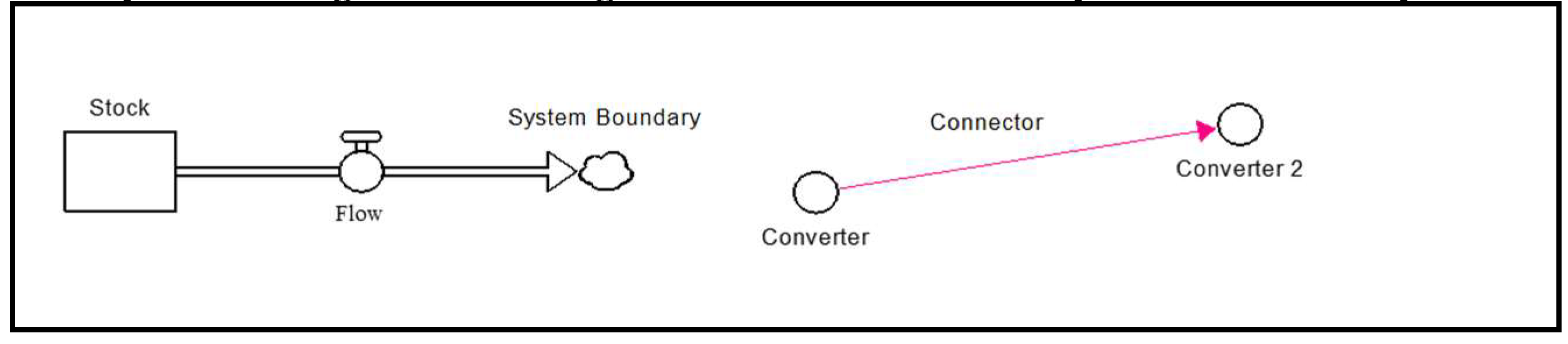
Figure 2.
Supply chain model of manufacturing process of hemp reinforced composite material.
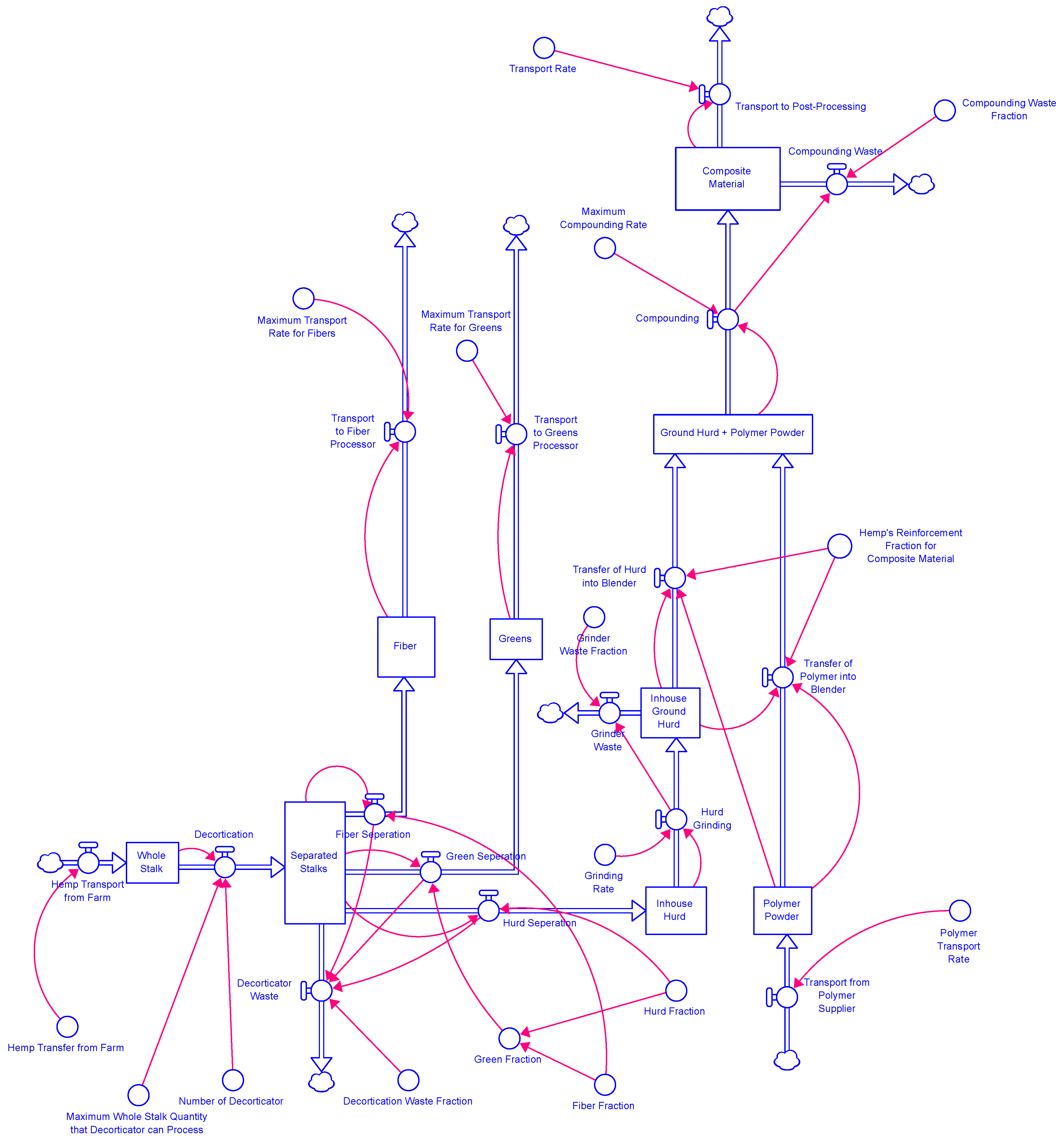
Figure 3.
Flows entering and exiting the stock, Whole Stalk.
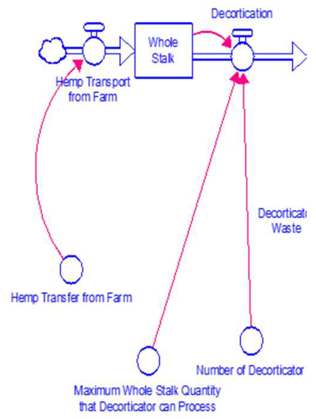
Figure 4.
Initial simulation.
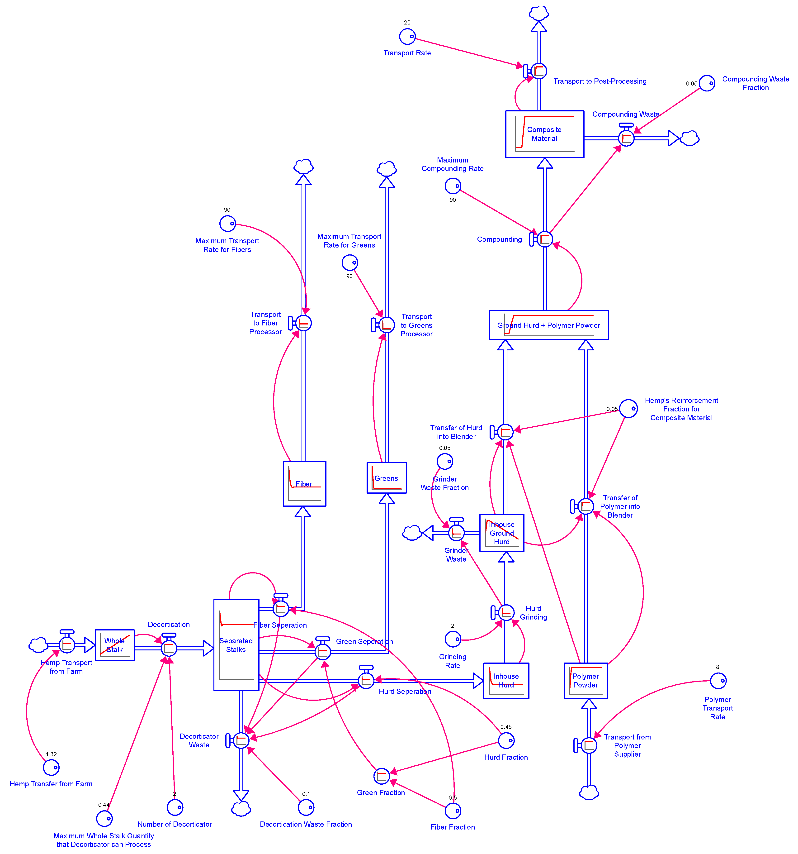
Figure 5.
Stable simulation.
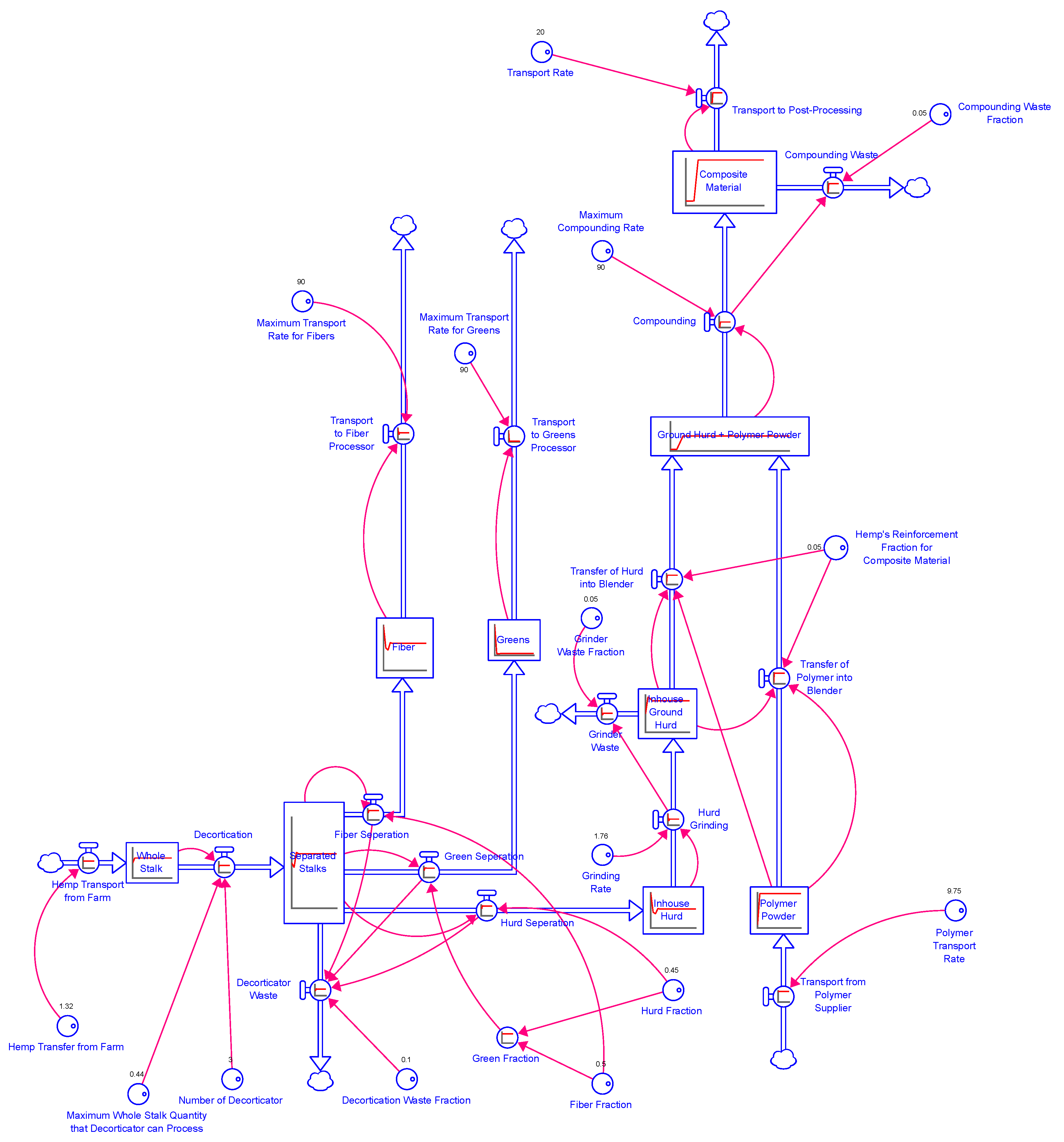
Table 1.
Stocks.
|
Serial Nos. |
Stocks |
Description |
| 1 | Composite Material | Quantity of hemp-reinforced polymer composite material produced |
| 2 | Fiber | Separated quantity of fiber after the decortication of the whole stalk |
| 3 | Greens | Separated quantity of greens after the decortication of whole stalk |
| 4 | Ground Hurd + Polymer Powder | Mix quantity of ground hurd and polymer powder to produce composite material |
| 5 | Inhouse Ground Hurd | Quantity of inhouse ground hurd after grinding inhouse hurd |
| 6 | Inhouse Hurd | Quantity of in-house hurd after separating greens and fiber from the whole stalk through decortication. |
| 7 | Polymer Powder | Quantity of polymer powder bought from polymer supplier to produce composite material. |
| 8 | Separated Stalks | Quantity of separated stalk after the decortication of whole stalk. |
| 9 | Whole Stalk | Quantity of the whole stalk bought into the unit from hemp farm for producing composite material. |
Table 2.
Converters.
|
Serial Nos. |
Converters | Description | |
| 1 | Compounding Waste Fraction | The fraction of compounding material waste generated from the compounding process | |
| 2 | Decortication Waste Fraction | The fraction of decorticating waste generated from the decortication of whole stalks. | |
| 3 | Fiber Fraction | The fraction of fiber separated from whole stalks after decortication. | |
| 4 | Green Fraction | The fraction of green separated from whole stalks after decortication. | |
| 5 | Grinder Waste Fraction | The fraction of grinder waste generated from hurd grinding. | |
| 6 | Grinding Rate | Rate at which inhouse hurd is grinded. | |
| 7 | Hemp Transfer from Farm | The quantity of hemp transferred from the farm into the factory. | |
| 8 | Hemp's Reinforcement Fraction for Composite Material | The reinforcement fraction of hemp to produce composite material. | |
| 9 | Hurd Fraction | The fraction of hurd separated from whole stalks after decortication. | |
| 10 | Maximum Compounding Rate | Maximum rate at which inhouse ground hurd and polymer powder are compounded. | |
| 11 | Maximum Transport Rate for Fibers | Maximum rate at which fibers are transported to post-processor. | |
| 12 | Maximum Transport Rate for Greens | Maximum rate at which greens are transported to post-processor. | |
| 13 | Maximum Whole Stalk Quantity that Decorticator can Process |
The maximum quantity that the decorticator can process. | |
| 14 | Number of Decorticators | The number of decorticators required. | |
| 15 | Polymer Transport Rate | The quantity of polymer transported into the factory. | |
| 16 | Transport Rate | The quantity of composite material transported to post-processor. | |
Table 3.
Flows.
|
Serial Nos. |
Flows | Description |
| 1 | Compounding | Rate at which mixture of ground hurd and polymer powder is compounded. |
| 2 | Compounding Waste | Rate of waste generation by compounding. |
| 3 | Decortication | Rate at which the whole stalk is decorticated. |
| 4 | Decorticator Waste | Rate of waste generation from decortication process. |
| 5 | Fiber Separation | Rate at which fiber is separated from the whole stalk. |
| 6 | Green Separation | Rate at which green is separated from the whole stalk. |
| 7 | Grinder Waste | Rate of waste generation from grinding inhouse hurd. |
| 8 | Hemp Transport from Farm | Quantity of hemp transported into the factory from the hemp farm. |
| 9 | Hurd Grinding | Rate at which inhouse hurd is grinded. |
| 10 | Hurd Separation | Rate at which hurd is separated from the whole stalk. |
| 11 | Transfer of Hurd into Blender | Rate at which inhouse ground hurd is transferred into blender. |
| 12 | Transfer of Polymer into Blender | Rate at which polymer is transferred into blender. |
| 13 | Transport from Polymer Supplier | Quantity of polymer transported into the factory from polymer supplier. |
| 14 | Transport to Fiber Processor | Quantity of fiber transported to fiber processor. |
| 15 | Transport to Greens Processor | Quantity of greens transported to greens processor. |
| 16 | Transport to post-processing | Quantity of composite material transported to post-processing unit. |
Table 4.
Converters in Figure 3.
Table 4.
Converters in Figure 3.
|
Serial Nos. |
Converters | Converter’s Variable Name | Unit |
| 1 | Hemp Transfer from Farm | Hemp_Transfer_from_Farm | Tons/day |
| 2 | Maximum Whole Stalk Quantity that Decorticators can Process |
Maximum_Whole_Stalk_Quantity_that_Decorticators_can_Process | Tons/day |
| 3 | Number of Decorticators | Number_of_Decorticators | Unitless |
Table 5.
Flows in Figure 3.
Table 5.
Flows in Figure 3.
|
Serial Nos. |
Name of the Flow | Equations | Unit |
| 1 | Hemp Transport from Farm | Hemp_Transfer_from_Farm | Tons/day |
| 2 | Decortication | IF((Whole_Stalk/DT)<Maximum_whole_stalk_quantity_that_decorticators_can_process * Number_of_Decorticators) THEN (Whole_Stalk/DT) ELSE (Maximum_whole_stalk_quantity_that_decorticator_can_process * Number_of_Decorticators) | Tons/day |
Table 6.
Stock in Figure 3.
Table 6.
Stock in Figure 3.
|
Serial Nos. |
Name of the Stock | Equation of Stock | Unit |
| 1 | Whole Stalk | Whole Stalk (t-dt) + Hemp Transport from Farm (t) – Decortication (t) | Tons |
Table 7.
Converter inputs for initial simulation.
|
Serial Nos. |
Converters | Initial Simulation’s Converter/ Input Values | Unit |
| 1 | Compounding Waste Fraction | 0.05 | Unitless |
| 2 | Decortication Waste Fraction | 0.1 | Unitless |
| 3 | Fiber Fraction | 0.5 | Unitless |
| 4 | Green Fraction | 0.05 | Unitless |
| 5 | Grinder Waste Fraction | 0.05 | Unitless |
| 6 | Grinding Rate | 2 | Tons/day |
| 7 | Hemp Transfer from Farm | 1.32 | Tons/day |
| 8 | Hemp's Reinforcement Fraction for 3D Printed Final Product |
0.05 | Unitless |
| 9 | Hurd Fraction | 0.45 | Unitless |
| 10 | Maximum Compounding Rate | 90 | Tons/day |
| 11 | Maximum Transport Rate for Fibers | 90 | Tons/day |
| 12 | Maximum Transport Rate for Greens | 90 | Tons/day |
| 13 | Maximum Whole Stalk Quantity that Decorticator can Process | 0.3 | Tons/day |
| 14 | Number of Decorticators | 2 | Unitless |
| 15 | Polymer Transport Rate | 8 | Tons/day |
| 16 | Transport Rate | 20 | Tons/day |
Table 8.
Converter inputs for stable simulation.
| Converters | Stable Simulation Converter/Input Values | Unit | |
| 1 | Compounding Waste Fraction | 0.05 | Unitless |
| 2 | Decortication Waste Fraction | 0.1 | Unitless |
| 3 | Fiber Fraction | 0.5 | Unitless |
| 4 | Green Fraction | 0.05 | Unitless |
| 5 | Grinder Waste Fraction | 0.05 | Unitless |
| 6 | Grinding Rate | 1.76 | Tons/day |
| 7 | Hemp Transfer from Farm | 1.32 | Tons/day |
| 8 | Hemp's Reinforcement Fraction for 3D Printed Final Product |
0.05 | Unitless |
| 9 | Hurd Fraction | 0.45 | Unitless |
| 10 | Maximum Compounding Rate | 90 | Tons/day |
| 11 | Maximum Transport Rate for Fibers | 90 | Tons/day |
| 12 | Maximum Transport Rate for Greens | 90 | Tons/day |
| 13 | Maximum Whole Stalk Quantity that Decorticator can Process |
0.44 | Tons/day |
| 14 | Number of Decorticators | 3 | Unitless |
| 15 | Polymer Transport Rate | 9.75 | Tons/day |
| 16 | Transport Rate | 20 | Tons/day |
| Serial Nos. (from their respective tables) | Converters | Initial Simulation Converter/Input Values | Stable Simulation Converter/Input Values |
| 6 | Grinding Rate | 2 | 1.76 |
| 13 | Nos of Decorticators | 2 | 3 |
| 15 | Polymer Transport Rate | 8 | 9.75 |
Disclaimer/Publisher’s Note: The statements, opinions and data contained in all publications are solely those of the individual author(s) and contributor(s) and not of MDPI and/or the editor(s). MDPI and/or the editor(s) disclaim responsibility for any injury to people or property resulting from any ideas, methods, instructions or products referred to in the content. |
© 2024 by the authors. Licensee MDPI, Basel, Switzerland. This article is an open access article distributed under the terms and conditions of the Creative Commons Attribution (CC BY) license (http://creativecommons.org/licenses/by/4.0/).
Copyright: This open access article is published under a Creative Commons CC BY 4.0 license, which permit the free download, distribution, and reuse, provided that the author and preprint are cited in any reuse.


