
Submitted:
03 December 2024
Posted:
04 December 2024
You are already at the latest version
Abstract
EU regulations get stricter from 2028 on by imposing net-zero energy building (NZEB) standards on new residential buildings including on-site renewable energy integration. Heat pumps (HP) using thermal building mass, and Model Predictive Control (MPC) provide a viable solution to this problem. However, the MPC potential in NZEBs considering the impact on indoor comfort have not yet been investigated comprehensively. Therefore, we present a co-simulative approach combining MPC optimization and IDA ICE building simulation. The demand response (DR) potential of a ground-source HP and the long-term indoor comfort in an NZEB located in Vorarlberg, Austria over a one year period are investigated. Optimization is performed using Mixed-Integer Linear Programming (MILP) based on a simplified RC model. The HP in the building simulation is controlled by power signals obtained from the optimization. The investigation shows reductions for electricity cost by up to 49% for HP, by up to 5% for the building, and an increase of the PV self-consumption by up to 4% pt. in two distinct optimization scenarios. Moreover, compared to the reference PI controller, the MPC scenarios provided more consistent and more reliable indoor comfort by reducing fluctuating room temperatures and maintaining stable indoor conditions. Especially precooling strategies mitigated overheating risks in summer and ensured indoor comfort according to EN 16798-1 class II standards.
Keywords:
Heat Pump
; Model Predictive Control (MPC)
; Mixed-Integer Linear Programming (MILP)
; PV Self-Consumption
; Demand Response
; Net-Zero Energy Building (NZEB)
; Building Simulation
1. Introduction
In recent decades, policymakers have tightened building efficiency standards and promoted on-site energy generation through concepts like nearly zero-energy buildings (nZEB) and net-zero energy buildings (NZEB). This aims to reduce the carbon footprint of buildings, which currently account for nearly 30% of global CO2 emissions [1]. However, latest reports by the International Energy Agency show that the building sector is not on the desired track to significantly improve energy efficiency [1]. In the European Union (EU), a key regulation in the recast (2024) of the Energy Performance of Buildings Directive mandates that all new buildings must be zero-emission buildings based on least nZEB standards starting from 2028. Thus, zero-emission buildings must provide on-site renewable energy generation and flexibilities like electric and thermal energy storages [2]. So far, the national definitions of nZEB in EU countries are shaped by both, technical and political factors. Thus, they vary and are often difficult to compare [3,4]. In contrast, a NZEB is clearly defined as one where on-site energy generation equals the building’s consumption, balancing out its energy use over a one year period [5]. However, ambiguities in the evaluation can lead to unclear results that do not allow for subsequent comparison. As example, evaluating NZEBs on an annual basis can lead to buildings with oversized PV systems and/or high energy needs, where the surplus energy generated in summer compensates for the rest of the year. Thus, imposing significant stress on the grid as on-site energy generation continues to grow [6]. Various factors are explored in the literature to optimize NZEB design and operation. Belussi et al. [7] emphasize the importance of considering the building envelope, the internal gains, and the HVAC systems during optimization. In cold climates, a high-quality envelope is important to reduce energy consumption, whereas in mild climates (e.g. such as Central European Alpine Regions) external movable shadings are mandatory to prevent overheating [7]. Additionally, internal gains e.g., occupancy, equipment and lighting, have to be considered, as they lead to changes in room temperature and indoor comfort [8]. Heat pumps (HP) are the most commonly used HVAC technology in NZEBs [9] and play a significant role for renewable energy integration via advanced control strategies [10].
Demand Side Management (DSM) approaches represent such advanced control strategies to integrate on-site renewable energy production, while reducing energy costs, lowering emissions, and improving energy efficiency [11]. Demand response (DR) is one category of DSM, which involves methods to adjust energy demand, such as peak shaving, valley filling, and load shifting [12]. Research in DR often focuses on simple and robust methods, typically implemented using rule-based control (RBC) within building simulation tools such as IDA ICE or TRNSYS [13,14,15,16,17,18]. These approaches, involving on-off control or proportional-integral (PI) regulators, are practical and easy to apply, though they lack the predictive capabilities of more advanced methods like model predictive control.
To maximize the flexibility of HPs at the building level, the research community increasingly advocates for MPC as an effective approach [10,19,20,21]. MPC is particularly attractive due to its ability to address multiple objectives simultaneously [19]. Various studies have demonstrated the MPC potential in utilizing HPs for domestic hot water (DHW) and/or space conditioning, whether in simulation [22,23,24,25,26,27] or in field tests [28,29,30]. The simulations are commonly based on simplified RC models [22,23,24,25], which lack to represent the detailed building structure (according to specifications) and to evaluate the comfort within different zones. The same applies to field tests [29,30], as they are also often simplified and short-term for complexity reasons, even though they reproduce the realistic demand of the building and the energy consumption of the HP very well. Co-simulation concepts with building software aim to improve upon this by additionally investigating the thermal behavior including the indoor comfort using detailed building models [26,27,31,32,33,34]. As building simulation is computationally expensive, most studies comprise simplified representations of single [27,32,34] and multi-family houses [26,33], and perform short-term investigations.
For instance, Wei et al. [27] modeled a single-family house (SFH) as single zone in TRNSYS and an RC model in MATLAB to investigate the MPC potential within a winter period for different opaque structures and future climate scenarios. Thereby, the medium-weight building provided the best flexibility option with the lowest operation cost compared to the light-weight and the heavy-weight building structure. Furthermore, the PV self-consumption increased by 5% in the medium-weight scenario. Likewise, Fop et al. [34] modeled a single zone in BOPTEST framework and an RC model in Python to investigate two MPC scenarios, in which operation costs should be minimized and comfort ensured. Within the 2 week simulation, operational costs and comfort violations have been decreased by up to 20% and 82%, respectively. However, Péan et al. [26] focused on a multi-family house with a HP for space heating (SH), space cooling and DHW using a thermal energy storage as additional flexibility for operational cost optimization. The 38 zones have been modeled in TRNSYS, whereas the corresponding RC model and the optimization have been done in GAMS. Optimization results for one week in winter, summer and intermediate showed cost reductions up to 20%. Unexpected space cooling operations in summer occurred and have not been further investigated.
To summarize: The MPC potential for SFHs in the literature through simplified RC model simulations, experimental setups, and co-simulative approaches has been proven. Nevertheless, a detailed and comprehensive study combining the long-term thermal behavior of building zones, the impact on indoor comfort, and the evaluation of on-site renewable energy integration considering operational costs of NZEBs under realistic conditions has not been conducted.
We want to overcome this lack by considering the following aspects in a comprehensive study:
- A detailed and realistic NZEB simulation model.
- A fair comparison of an RBC and an MPC approach.
- Electrical energy costs and self sufficiency.
- Climatic and comfort challenges.
We achieve this by:
- Modeling the building in IDA ICE covering all components and specific characteristics of the real building based in the Central European Alpine region, which is used for simulation.
- Developing a co-simulative MPC optimization setup with Python and IDA ICE covering both, a two-story NZEB IDA ICE and an RC model featuring a PV system and a ground-source HP for heating and cooling via an underfloor distribution system (UDS).
- Optimizing based on an RC model in Python, which is derived from transient energy balances. The state space representation remains linear with piece-wise constant parameters, enabling the use of MILP methods, resulting in a computationally efficient algorithm that ensures a global optimum.
- Addressing the prediction uncertainties and external disturbances via a formulation of the optimization problems within the MPC framework developed.
- Using the thermal mass of the building to serve as flexibility for DR. Exploiting this load-shifting potential in two separate scenarios, we optimize to increase the PV self-consumption and to reduce the total electrical energy costs.
2. Methodology
2.1. Simulation Study Concept
This study investigates a MPC strategy of a ground-source HP in a realistic NZEB covering the two optimization scenarios: 1) Increase of PV self-consumption (SC) and 2) reduction of electricity cost using real-time prices (RTP). The SFH is modeled in detail in IDA ICE, which is a dynamic simulation software developed by the Swedish company EQUA [35]. IDA ICE is widely recognized for its capability to model indoor climate, energy usage, and occupant comfort, allowing for detailed analysis of HVAC systems, energy consumption, and overall building performance. This makes it a valuable tool for energy-efficient building design and optimization. The simulation utilizes data from 2023. For optimization using MILP in Python, a simplified RC model of the SFH is developed. The simplified RC model, along with the optimizer, is then employed to optimize the HP control within the detailed IDA ICE simulation framework as part of an MPC approach. The MPC concept for this co-simulation is illustrated in Figure 1.
The optimization inputs include the current state of the rooms delivered from IDA ICE and external data. The state includes room temperatures, whereas the external data include information about the weather (solar radiation and ambient temperature), the RTP [36], the internal gains and the electric base load. According to the optimization objectives, the algorithm optimizes the HP control and the building’s heating and cooling operations by calculating future thermal loads and energy costs and delivers the achieved control signals back to IDA ICE. This interaction leverages the predictive capabilities of the MPC, allowing it to anticipate future conditions and adjust the operation of the HP, while ensuring indoor comfort. The integration of IDA ICE within this co-simulation framework enhances the flexibility and accuracy of the control strategy, enabling a robust evaluation of MPC performance. The optimization scenarios are compared with a reference case using a PI-control strategy. The PI-controller continuously regulates the thermal HP output to minimize the error between the actual room temperature and the desired set-point, ensuring smooth operation without abrupt on/off switching. Set-points for heating and cooling temperatures are chosen according to EN 16798-1 [37]. This minimizes cycling, reducing inefficiencies and wear while maintaining comfort. However, the PI-control strategy can lead to suboptimal energy use and indoor comfort, especially with rapid changing weather, which the dynamic MPC strategy aims to improve on.
2.2. IDA ICE System Overview
The study employs an IDA ICE model to simulate the thermal behavior of a real-life NZEB located in Vorarlberg, Austria (cf. Figure 2). The model is based on specifications from the building’s Energy Performance Certificate (an official, mandatory document in the EU to evaluate a building’s energy efficiency according to [39,40], cf. HERS rating in the US), accurately representing the building envelope, including walls, roof, and floors (cf. Table 1). Further, key elements of the system include the following:
- Heating and Cooling System: A ground-source HP system is modeled, providing heating and cooling through UDS.
- Photovoltaic System: A 6.7 kWp PV system is included, providing power for the HP system and the internal use, and further reflecting the building’s renewable energy generation capacity.
- Internal Gains: Internal heat gains from equipment, occupants, and lighting are considered based on typical residential usage patterns (cf. Table 2).
DHW demand is integrated into the buildings base load to focus the analysis on the building’s heating and cooling performance. The model closely mirrors the real-life building, ensuring accurate and relevant simulation results.
2.2.1. IDA ICE Building Model
The real-life building captures the thermal performance standards required for NZEBs using components with low U-values (cf. Table 1). The use of insulated timber frames, wood fiber insulation, and multiple layers in walls, floors, and ceilings creates a highly resistant building envelope with minimized thermal bridging and heat loss.
The IDA ICE model of the NZEB consists of key structural elements, including the base plate with flooring, external walls, windows, floor/ceiling assembly, and the roof (specifics, cf. Table 1). The base plate with flooring with an area of 90 m2 includes layers such as reinforced concrete, bituminous sheeting, leveling screed, thermal insulation, cement screed with a vapor barrier, and flooring. These layers total 0.58 m in thickness, achieving a U-value of 0.16 W/(m2 K), providing high thermal resistance to reduce ground heat loss.
The external walls vary in orientation and floor level, utilizing a timber-framed structure with wood fiber insulation to minimize heat transfer. These walls have areas ranging from 8.8 to 23.4 m2 on the first and second floor and are composed of a 0.46 m-thick assembly of timber framing, wood fiber insulation, and plasterboard, achieving a U-value of 0.10 W/(m2 K) in line with NZEB requirements.
Windows are strategically placed across the building’s facades with areas ranging from 0.7 to 17.2 m2 and are equipped with time-variant controlled external blinds. Larger windows are positioned on the south side to take advantage of passive solar gains in winter, reducing the need for heating, whereas windows on other sides help balance natural lighting while preventing excessive heat gain. All windows are made of insulated glazing with a thickness of 0.008 m and a U-value of 0.74 W/(m2 K). Window ventilation is neglected in this study to avoid additional disturbances for the model and reduce complexity.
The floor/ceiling assembly spans the first and second floors, with a total area of 90 m2. It includes layers of flooring, cement screed with a vapor barrier, a thermal insulation panel with impact sound insulation, an insulated timber frame with oriented strand board, and plasterboard. This structure has a thickness of 0.5 m and a U-value of 0.165 W/(m2 K). The roof consists of a board stacked ceiling, wood insulation with a vapor barrier, and a vapour-permeable wood fiber board.
The 6.7 kWp PV system (PV panels Jinko JKM280M-60B) is oriented southwards with a tilt angle of 25°.
Additionally, internal gains are especially significant to consider in NZEBs, as occupants, equipment, and lighting contribute substantially to the heat load of the building. The profiles used in this study are categorized into occupancy, equipment, and lighting and apply to each floor (cf. Table 2). The SFH accommodates four occupants (1.0 MET and 0.8 CLO) with heat gains via lighting and equipment of 4.6 W/m2, accordingly to [37,41]. Table 2 shows the respective schedules, powers, heat gains, activity levels of the occupants, and annual energy values.
2.2.2. IDA ICE Heat Pump System Model
The heating/cooling system is modeled via a reversible ground-source HP that enables both heating and cooling through an UDS (cf. Figure 4). The HP covers a maximum heating and cooling load of 5.5 kW and 2.5 kW, respectively. The Coefficient of Performance and the Energy Efficiency Ratio total in 4.0 for each indicator, respectively. In the reference case, the HP control logic follows a PI-controlled strategy, where a certain room temperature of each zone (season dependent) has to be maintained, and thus, a certain demand to be satisfied. The gradient of each room temperature depends on the energy input given by the UDS circuit of each zone. To maintain the thermal comfort by preventing overheating and undercooling, an upper and lower threshold of 26 °C and 21 °C according to class II EN 16798-1 [37] are set, respectively. In the MPC case, the HP control logic follows a control signal given by the optimization, controlling the energy input/output to the rooms via the UDS. The supply temperature of the heating and cooling circuits are regulated to 35 °C and 18 °C, respectively.
The model is focusing solely on space conditioning. This configuration allows for a realistic simulation of the HP performance without introducing the complexities by an additional thermal energy storage or operation for DHW production.
2.3. Modeling
For modeling, the two-story building is divided into two floors with one room and one envelope part, respectively. Each room (room 1 and 2) is representing the thermal capacitance of the indoor air ( and ) and each building envelope part the thermal capacitance of the opaque structures (wall, floor, ceiling and roof) of the house ( and ), respectively. The room temperatures ( and ) depend on the thermal energy exchange with the building’s envelope parts, the internal gains (), and the heat input through solar radiation () controlled by external blinds with a shading variable (). The building envelope temperatures ( and ) represent the mean temperature in the opaque structure and depend on the heat input through solar radiation (), the heating and cooling power ( and ) by the HP, as well as the thermal energy exchange with the ambient () and each envelope part to each other. The thermal energy flows are modeled via conduction leading to the RC model from Figure 5. Given the high level of insulation in the opaque structure of the NZEB, thermal energy flows are primarily expected to occur between the building envelope and the interior, rather than being significant between the envelope and the ambient environment. In addition, window ventilation is neglected to avoid additional disturbances and reduce complexity.
The overall heating/cooling powers of the HP ( and ) are calculated by using the electrical power (), coefficient of performance (), and the energy efficiency ratio (). The distribution of the overall heating and cooling power to each heating/cooling circuits (, , and ) within each building envelope part are calculated as follows:
The thermal influence of the sun is modeled for each subpart with the incident solar radiation (, , and ), which is assumed to heat the building envelopes and the rooms. The incident solar radiation is calculated by using the global solar radiation () and a solar exposure factor () as follows:
As addition to the rooms, a time-variant factor for the shading control () has to be considered, as blinds influence the incident solar radiation significantly. The internal gains and for room 1 and 2, respectively consist of the gains from lighting, equipment, and occupancy.
The heat transfer rates from the building envelope to the rooms, to the ambient and to each other are modeled using single heat transfer characteristics (k) to reflect heat conduction via the opaque structure with it’s given U-values (cf. Table 1). The equations representing the heat flows are given by:
where and are the heat flows from the single rooms to the single building envelope part, and are the heat flows from the building envelope parts to ambient, and is the heat flow from the building envelope 1 to 2.
Assuming , , , , , , , , , , , and to be constant in each time interval, this defines a system of first-order inhomogeneous linear ordinary differential equations (ODEs) with constant coefficients for every time period. The system of ODEs for one time period can be given in the following form:
Let represent the coefficient matrix, while denotes the inhomogeneous term, where is the control vector that will later serve as the decision variable in the optimization problem. These ODEs describe the state space of the system and can be solved using the matrix exponential along with the steady-state solution , expressed as follows:
This solution can be applied for piece-wise constant parameters on N intervals of duration leading to:
By utilizing this analytical solution, the system dynamics can be computed at all time points, indexed by .
To fit the model to represent the system dynamics, a Prediction Error Method (PEM) is used to identify the system parameter of the building in a defined reference scenario. The PEM uses the least squares optimization, where the sum of the quadratic errors of the IDA ICE simulated and the RC estimated temperatures of both rooms are minimized via
2.4. Optimization
The optimization objectives in the two distinct scenarios are: 1) Increase of PV self-consumption and 2) reduction of the electricity cost using RTP. To obtain the optimization objectives, load shifting is applied using the thermal mass of the building as flexibility. This flexibility allows to shift the cooling or heating power of the HP to times with a surplus of PV power (scenario 1) or lower energy prices (scenario 2), while maintaining indoor comfort. MILP is chosen as optimization method according to [42], because it is computationally very efficient and solutions are guaranteed to be the global optimum for passive energy storages such as thermal building mass. The requirement for MILP is a piece-wise linear system, which is fulfilled by the model from Section 2.3. The optimization interval is one hour and the data used is described in Section 3.2. The problem is formulated using the following decision variables:
- and is the cooling power via building envelope for room 1 and room 2 during the time period p, respectively.
- and is the heating power via building envelope for room 1 and room 2 during the time period p, respectively.
- is the electrical heat pump power during the time period p.
- is the total electrical grid power during the time period p, where positive values indicate consumption.
- is the electrical power consumed from the grid during the time period p.
- is the electrical power feed-in to the grid during the time period p.
- is a binary variable indicating if power is consumed during the time period p.
- is a binary variable indicating if power is feed-in during the time period p.
- is a binary variable indicating if the HP is in the cooling mode during the time period p.
- is a binary variable indicating if the HP is in the heating mode during the time period p.
- is a column vector for the temperatures consisting of , , and . and are the temperatures of room 1 and 2 at time point i, respectively. and are the temperatures of building envelopes 1 and 2 at time point i, respectively.
- is the steady state solution according to Equation (22) during time period p.
- is the control vector. It is a column vector according to Equation (21) with the heating and cooling powers and their efficiencies during the time period p.
Note that , , and are the decision variables relevant for operation, while the auxiliary variables help to improve the readability of the formulation. The following input time series are needed:
- is the PV power during the time period p.
- is the electrical base load during the time period p.
- is the price signal for consumption during the time period p.
- is the price signal for feed-in during the time period p.
- is a column vector of the matrix form according to Equation (21) during time period p representing the model inputs such as ambient temperature or the internal gains.
The following parameters are needed:
- is the length of a time period.
- is the energy efficiency ratio of the HP for cooling.
- is the coefficient of performance of the HP for heating.
- is the maximum cooling power of the HP.
- is the maximum heating power of the HP.
- and are lower bounds of the room temperature of room 1 and 2, respectively.
- and are upper bounds of the room temperature of room 1 and 2, respectively.
- is a column vector with the initial temperatures of at the time point .
- is the coefficient matrix according to Equation (21).
- N is the number of time periods.
- M is used for a big M constraint.
The following sets are defined:
- is the set of the time period indices.
- is the set of the time point indices.
The optimization problem can be written as:
The objective function defined in Equation (26) describes the optimization objective for both scenarios. To obtain the different outcome according to the objectives, the price signals for consumption and feed-in have to be adjusted. To increase PV self-consumption, the consumption and feed-in prices are set to and , respectively. Consequently, the energy consumed by the grid is minimized and as much as possible PV power surplus used instead. If the PV surplus is not enough to satisfy the demand, energy is consumed by the grid. Otherwise, if there is still PV surplus available after all consumption, the surplus of PV power will be fed into the grid. To decrease the total energy costs, real-time prices for and are applied. As RTP fluctuate over time, the optimization will ensure that the energy is consumed in times prices are lowest. In lines (,) the sets of the periods and time points are defined. N time periods lead to time points. Note that the state variable is continuously changing and is indexed with the time points i from , while other variables such as the prices, heating/cooling powers or electrical powers are piece-wise constant inputs or process variables and indexed via the time periods p from . Equation () describes the energy balance of the electrical part of the system and Equation () splits the grid power into the positive part and the negative part of its value, which is needed for the objective function if the prices for energy consumption and feed-in differ. Equations (-) ensure that the system can not consume and feed-in energy at the same time. Due to the non-linearity of that function, it is piece-wise linearized using binary variables and the big M constraint. The electrical power of the HP is calculated in Equation (). Equations (-) limit the maximum cooling or heating powers and ensure that the HP is either in cooling mode or in heating mode. The room temperatures and are constrained in Equations (,) and the starting temperatures of the system are defined in Equation (). Equations (,) are the transient thermal energy balance according to the model from Section 2.3. Last, the variable types are defined by Equations (-). This optimization problem is implemented in the MPC concept. Note that the start values of the room temperatures , are received as simulated values after every optimization from IDA ICE. Information about the building’s envelope initial temperatures and are usually not available in real systems. Therefore, the values from IDA ICE are not used and instead starting values are calculated according to the ODE. To avoid that the calculated values of the building envelope , drift too far away in a long-term simulation due to model inaccuracies, it is assumed that at midnight the building temperatures can be approximated by the room temperatures. That is why always at midnight, the values for , are used to initialize , .
3. Results
3.1. NZEB Case Study
In the reference scenario, data for the entire year 2023 are available. The one-year simulation comprises seasonal variations in heating, cooling, PV production, energy use and also covers occupancy, equipment and lighting schedules. The hourly data include room temperatures (room 1 and room 2), PV power, the building base load, HP compressor power for heating/cooling, grid consumed power, sold and self-consumed energy.
The reference scenario (REF) (cf. Figure 6 and Table 4) shows that the produced energy by PV (6204 kWh) could cover the whole amount of energy used in the building over the year (5856 kWh). Due to the mismatch of production and use, two-thirds of the used energy is purchased from the grid (3888 kWh) and likewise two-third of the produced energy sold (4236 kWh). Hence, an effective self-consumption is not possible in the reference and shows load shifting potential for the MPC approach proposed.
For the MPC optimization routine in Section 3.2, the RC model needs to be parametrized. Table 3 shows the model parameters identified from the reference scenario. The parameters comprise the thermal capacitance of both rooms ( and ) and the building envelope ( and ), the heat transfer coefficients between rooms, envelope, and outside (, , , , ) and the solar exposure factor for each room and envelope part (, , , ). The R2 scores of room 1 with and room 2 with yield 0.80 and 0.97, respectively. Figure 7 (left) shows the accuracy according to the R2 scores of the estimated and simulated temperatures for room 1 (top) and room 2 (bottom) within a three-day example. Box plots of the squared residuals (cf. Figure 7, right top and bottom) illustrate the estimation errors in room temperatures over one year. Accordingly to the lower results of the R2 score of 0.80, room 1 shows a ten times higher median value and variability (up to 1.0 K2) compared to room 2 (below 0.1 K2).
3.2. Analysis of MPC Potential
To verify the MPC potential, data of the reference scenario REF and two MPC scenarios (RTP and SC) for the whole year 2023 are considered. The data are compared with respect to: 1) total HP operation cost, 2) HP operation cost per unit electricity, 3) total HP electricity consumption, 4) HP electricity consumption for heating, 5) HP electricity consumption for cooling, 6) total electricity cost of the building, 7) used energy, 8) electricity consumption from grid, 9) PV self-consumption ratio, 10) self-sufficiency ratio, and 11) comfort criteria (average and maximum PPD), cf. Table 4. Thereby, the PV self-consumption ratio is defined as the proportion of the total electricity generated by the PV system that is consumed on-site directly by the electrical loads from the building including the HP relative to the total PV generation. Further, the self-sufficiency ratio is the proportion of the total electricity consumption by the building including the HP that is met directly by on-site PV generation without reliance on grid-supplied electricity. It quantifies the degree of independence from external energy sources. The EXAA day-ahead price of 2023 [36] including grid fees is applied as consumption tariff for all scenarios. The feed-in tariff is set to zero to represent the continuously decreasing prices and to focus on self-consumption. Additionally for both optimization scenarios, model inputs assuming perfect predictions include weather data (solar radiation and ambient temperature), estimates of internal gains, and the electrical base load.
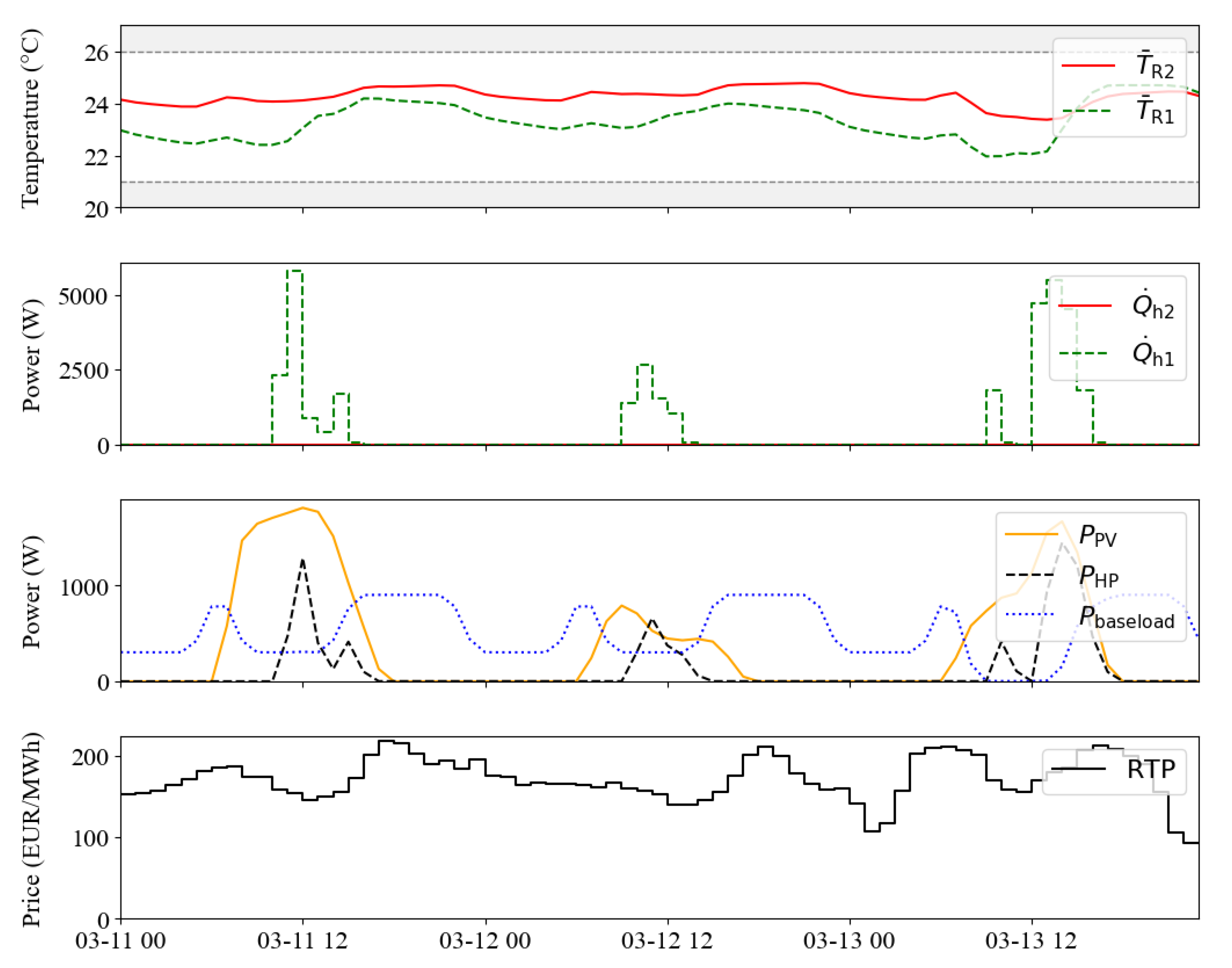
To show the viability of the MPC routine, Figure 8 presents three example days of the SC scenario from June 17 to June 19. While the top plot shows the maintained indoor temperatures for both rooms within the desired comfort range, sub plot 3 shows the ability of the MPC to shift the HP load to times with a surplus of PV power. A surplus of PV power is available if the building base load is already covered. If there is no power surplus available, the MPC routine will switch the HP in times, where the RTP is lowest within the predicted horizon (cf. HP power at 7am on 17th of June, sub plot 3 and 4). Analogously, a three day example of the optimization routine of the RTP scenario can be found in Appendix Figure A1.
Summarized on a yearly basis, the RTP and the SC scenario save HP operation cost per unit electricity compared to the reference scenario of 47.91% and 49.26%, respectively (cf. Table 4). Despite the drastically decrease in cost, the HP electricity consumption increases by 2.33% and 3.43% for RTP and SC, respectively. In particular, the cooling operation contributes with +27.09% for RTP and +28.39% for SC to a major extend to the overall increase in HP electricity consumption, which is further discussed in Section 3.3. The HP contributes with roughly 11% only to a small extend to the overall building load (cf. Figure 6). Consequently, the total electricity cost decrease by just 4.84% and 4.94% for RTP and SC, respectively. Further, the overall used energy increases by 1.13% (RTP) and 1.26% (SC). However, the aim to increase the self-consumption and the self-sufficiency is ensured. The self-consumption ratio increased by 3.82% pt. and 4.12% pt. for RTP and SC, respectively. Likewise, the self-sufficiency ratio increased by 3.63% pt. (RTP) and 3.91% pt. (SC).
3.3. Comfort Conditions
Comfort criteria according to class II EN 16798-1 [37] are applied in this study. This means, the room temperature should not exceed 26°C more than 25% of the time simulated. Likewise, the lower bound should not deceed 21°C. As key metric the Predicted Mean Vote (PMV) and Predicted Percentage of Dissatisfied (PPD) are applied. The data for the probability density estimation is normalized and the bandwidth is adjusted.
Unlike the maintained comfort for an average day between 5.90% up to 7.18% for all scenarios (cf. Table 4), the maintenance of stable temperatures conditions is difficult in worst case situations (e.g. very hot/cold days). Thereby, the control strategy has a major influence on maintaining comfort additionally to passive measures. The PI regulator (REF) continuously adjusts the heating/cooling output based on the difference between the set-point and the actual room temperature, resulting in less thermal losses than preheating/precooling the building. Hence, the HP needs 2-3% more energy in RTP and SC than in the REF scenario (cf. Table 4). However, this short-term control leads to comfort losses, if the environmental conditions face a rapid change or push the HP system to its maximum capacity. Figure 9 shows exactly this behavior for REF, as the mean PPD and mean PMV for room 2 are at the comfort border to 10% and 0.5, respectively. Especially in summer, room 2 tends to strong overheating and violates comfort acc. to class II EN 16798-1 [37], if no precooling or window ventilation is applied (cf. Figure 9, b)). The MPC counteracts to this problem by preheating and precooling the rooms within the specified temperature range (21 °C to 26 °C) such that the comfort is met. This leads to a decrease in the mean PPD of approx. 2-3% pt. for both rooms and both MPC scenarios compared to the reference. The density of the violins indicate only a few values above 10% PPD for border cases in RTP and SC scenario, which are allowed according to EN 16798-1. However, the precooling in the RTP and SC scenario increases the energy consumption for cooling by 27.09% and 28.39%, respectively. The same applies for preheating, increasing the energy consumption for heating by 1.68% and 2.82%, respectively. In general it is worthy to note, that to maintain indoor comfort during summer in NZEBs in alpine region (cf. Figure 9, b)), cooling is necessary, if no proper window ventilation and more advanced shading control is applied. According to the Austrian building guideline OIB6 [40] cooling for NZEBs should be avoided and proper passive measures preferred.
Figure 10 shows the most critical single comfort violations obtained by the MPC in the RTP scenario. While in summer (Figure 10 bottom), the MPC generally ensures stable indoor comfort in both rooms, RC model uncertainties and high ambient temperatures on 10th of June lead to comfort violations in room 2 with a maximum PPD of 12.9%. Likewise, in winter the comfort for room 1 is violated with a maximum PPD of 19.1% due to flexibility use by heating in low price periods and model uncertainties (cf. Figure 10, top).
4. Practical Considerations
Through this study, several challenges associated with the indoor comfort conditions and the co-simulation framework were identified, which should be considered for practical reasons.
While MPC generally performs well and largely maintains room temperatures within the comfort boundaries, a few overheating issues are observed. One critical scenario is the overheating during a winter day (cf. Figure 10, top). This overheating behavior is not only inefficient due to high gradients against ambient, but also violates the occupants comfort. However, model inaccuracies and prediction errors can generally lead to miscalculation of heat demand and to the excessive heating behavior. As our scenarios are based on perfect predictions, a more robust and periodic model calibration, e.g., for each season, could help to minimize these inaccuracies and violations.
Further, overheating in summer remains a challenge especially for NZEBs due to the high insulation standards. Additionally to the comfort requirements within the EU according to EN 16798-1 [37], country-specific requirements have to be considered. For Austria, the OIB6 guideline [40] demands the prevention of active cooling in NZEBs and instead suggests passive measures such as shading control and free-cooling via window ventilation during night. The models in this study include shading control, but neglect window ventilation due to complexity reasons. Even though in MPC scenarios comfort violations can be reduced compared to the reference scenario (cf. Table 4), the precooling of the rooms led to increased electricity consumption for cooling by up to 28%. To counteract on both, excessive electricity consumption and comfort violations (even in the reference scenario), intelligent window ventilation should be applied and integrated into the models.
Apart from the integration of passive measures into the models, the trade-off between single-zone and multi-zone modeling poses a challenges in MPC implementation. Whereas multi-zone modeling provides greater accuracy by considering varying room usages and thermal preferences, single-zone models reduce computational complexity significantly, but may not capture the diverse thermal dynamics of different rooms. Selecting the appropriate level of model complexity involves balancing computational efficiency with the need for accurate representation of the building’s thermal behavior. Our study acts on this principles and reduces complexity to a two zone model to investigate long-term thermal behavior without neglecting NZEB relevant aspects, such as building structure characteristics, internal gains, underfloor distribution system and shading control.
5. Conclusions
EU regulations get stricter and oblige building owners to reduce emissions, renovate buildings and support on-site renewable energy integration. HPs with thermal building mass can provide additional flexibility through their ability to shift loads. NZEBs, as the current state-of-the-art, can provide an insightful baseline for possible potential and viable realization of load shifting. However, to date, a detailed and comprehensive co-simulative study on MPC of a space heating and cooling HP system under realistic conditions using building simulation of NZEBs has not been available.
Therefore, we showed for the first time how an MPC approach can be combined with building simulation to investigate the DR potential, the long-term thermal behavior of building zones, and the indoor comfort of an NZEB in the Central European Alpine region. We proposed a RC model for optimization, and the building software IDA ICE for simulation. The RC model is based on transient energy balances resulting in a linear state space representation of the system, where MILP is used for optimization. The properties of the MILP make the optimizations computationally efficient. We investigated two optimization scenarios containing the two objectives to 1) increase PV self-consumption of the HP and 2) to reduce the total electricity costs of the building using real-time prices.
The results quantify and validate the savings, as well as the DR potential, achievable by a co-simulate MPC approach in the two optimization scenarios compared to the reference control. Within the scenarios of our case study, the HP electricity costs were reduced by up to 49%, the total electricity cost by up to 5%, whereas the HP electricity consumption and the self-consumption ratio increased by up to 3% and 4% pt., respectively. Investigation on comfort according to class II EN 16798-1 [37] revealed a tendance for the overheating of NZEBs in Central European Alpine climate, which the MPC counteracts on with precooling, if no passive measures preferred according to the OIB6 [40] are applied. Consequently, MPC contributes to the stabilization of the indoor climate and comfort of NZEBs.
Therefore, further research in this area is of great interest. Promising further research directions include the implementation of additional building types based on the existing building stock as well as their application in different climate zones. The existing building stock, with its relatively high energy demand, could offer even greater DR potential worth investigating.
Author Contributions
Conceptualization, C.B., P.W. and P.K.; Methodology, C.B., P.W. and P.K.; software, C.B. and P.W.; validation, C.B.; formal analysis, C.B.; investigation, C.B.; resources, P.K.; data curation, C.B.; writing—original draft preparation, C.B.; writing—review and editing, C.B., P.W., W.S. and P.K.; visualization, C.B.; supervision, P.K.; project administration, C.B.; funding acquisition, P.K. All authors have read and agreed to the published version of the manuscript.
Funding
The financial support by the Austrian Federal Ministry for Digital and Economic Affairs and the National Foundation for Research, Technology and Development and the Christian Doppler Research Association is gratefully acknowledged.
Data Availability Statement
Data will be made available on request.
Acknowledgments
The authors are grateful to the project partner Gantner Instruments GmbH for providing data and information of the investigated household.
Conflicts of Interest
The authors declare no conflicts of interest. The funders had no role in the design of the study; in the collection, analyses, or interpretation of data; in the writing of the manuscript; or in the decision to publish the results.
Abbreviations
The following abbreviations are used in this manuscript:
| CLO | Clothing insulation |
| COP | Coefficient of Performance |
| DHW | Domestic Hot Water |
| DR | Demand Response |
| DSM | Demand Side Management |
| EER | Energy Efficiency Ratio |
| EU | European Union |
| HP | Heat Pump |
| HVAC | Heating, Ventilation, and Air Conditioning |
| MET | Metabolic equivalent of task |
| MILP | Mixed-Integer Linear Programming |
| MPC | Model Predictive Control |
| NZEB | Net-Zero Energy Building |
| nZEB | Nearly Zero-Energy Building |
| ODE | Ordinary Differential Equation |
| PEM | Prediction Error Method |
| PMV | Predicted Mean Vote |
| PPD | Predicted Percentage of Dissatisfied |
| PV | Photovoltaic |
| RBC | Rule-Based Control |
| RC | Resistor-Capacitor |
| REF | Reference |
| RTP | Real-Time Price |
| SC | Self-Consumption |
| SFH | Single-Family House |
| UDS | Underfloor Distribution System |
Appendix A
Appendix A.1
Figure A1.
Optimization results for three example days in winter, where MPC with RTP objective function is applied. Subplots from top to bottom represent: comfort criteria via room temperatures, heating load to zones, produced (PV) and used power (HP and base load), incentive function.
Figure A1.
Optimization results for three example days in winter, where MPC with RTP objective function is applied. Subplots from top to bottom represent: comfort criteria via room temperatures, heating load to zones, produced (PV) and used power (HP and base load), incentive function.
References
- International Energy Agency. Tracking Clean Energy Progress 2023. Technical report, International Energy Agency, 2023.
- European Parliament and the Council of the European Union. DIRECTIVE (EU) 2024/1275 OF THE EUROPEAN PARLIAMENT AND OF THE COUNCIL. Technical report, European Parliament and the Council of the European Union, 2024. http://data.europa.eu/eli/dir/2024/1275/oj, Accessed on 2024-09-25.
- Hermelink, A.; Schimschar, S.; Boermans, T.; Pagliano, L.; Zangheri, P.; Armani, R.; Voss, K.; Musall, E. Towards nearly zero-energy buildings - Definition of common principles under the EPBD - Final report. Technical Report ESDE1 0788, European Commission, 2013. [Google Scholar]
- D’Agostino, D.; Mazzarella, L. What is a Nearly zero energy building? Overview, implementation and comparison of definitions. Journal of Building Engineering 2019, 21, 200–212. [Google Scholar] [CrossRef]
- Marszal, A.; Heiselberg, P.; Bourrelle, J.; Musall, E.; Voss, K.; Sartori, I.; Napolitano, A. Zero Energy Building – A review of definitions and calculation methodologies. Energy and Buildings 2011, 43, 971–979. [Google Scholar] [CrossRef]
- Ochs, F.; Franzoi, N.; Dermentzis, G.; Monteleone, W.; Magni, M. Monitoring and simulation-based optimization of two multi-apartment NZEBs with heat pump, solar thermal and PV. Journal of Building Performance Simulation 2024, 17, 1–26. [Google Scholar] [CrossRef]
- Belussi, L.; Barozzi, B.; Bellazzi, A.; Danza, L.; Devitofrancesco, A.; Fanciulli, C.; Ghellere, M.; Guazzi, G.; Meroni, I.; Salamone, F.; Scamoni, F.; Scrosati, C. A review of performance of zero energy buildings and energy efficiency solutions. Journal of Building Engineering 2019, 25, 100772. [Google Scholar] [CrossRef]
- Elsland, R.; Peksen, I.; Wietschel, M. Are Internal Heat Gains Underestimated in Thermal Performance Evaluation of Buildings? Energy Procedia 2014, 62, 32–41. [Google Scholar] [CrossRef]
- Paoletti, G.; Pascual Pascuas, R.; Pernetti, R.; Lollini, R. Nearly Zero Energy Buildings: An Overview of the Main Construction Features across Europe. Buildings 2017, 7, 43. [Google Scholar] [CrossRef]
- Péan, T.Q.; Salom, J.; Costa-Castelló, R. Review of control strategies for improving the energy flexibility provided by heat pump systems in buildings. Journal of Process Control 2019, 74, 35–49. [Google Scholar] [CrossRef]
- Oskouei, M.Z.; Şeker, A.A.; Tunçel, S.; Demirbaş, E.; Gözel, T.; Hocaoğlu, M.H.; Abapour, M.; Mohammadi-Ivatloo, B. A Critical Review on the Impacts of Energy Storage Systems and Demand-Side Management Strategies in the Economic Operation of Renewable-Based Distribution Network. Sustainability 2022, 14, 2110. [Google Scholar] [CrossRef]
- Panda, S.; Mohanty, S.; Rout, P.K.; Sahu, B.K.; Parida, S.M.; Samanta, I.S.; Bajaj, M.; Piecha, M.; Blazek, V.; Prokop, L. A comprehensive review on demand side management and market design for renewable energy support and integration. Energy Reports 2023, 10, 2228–2250. [Google Scholar] [CrossRef]
- Bee, E.; Prada, A.; Baggio, P. Demand-Side Management of Air-Source Heat Pump and Photovoltaic Systems for Heating Applications in the Italian Context. Environments 2018, 5, 132. [Google Scholar] [CrossRef]
- Bee, E.; Prada, A.; Baggio, P.; Psimopoulos, E. Air-source heat pump and photovoltaic systems for residential heating and cooling: Potential of self-consumption in different European climates. Building Simulation 2019, 12, 453–463. [Google Scholar] [CrossRef]
- Pinamonti, M.; Prada, A.; Baggio, P. Rule-Based Control Strategy to Increase Photovoltaic Self-Consumption of a Modulating Heat Pump Using Water Storages and Building Mass Activation. Energies 2020, 13, 6282. [Google Scholar] [CrossRef]
- Thür, A.; Calabrese, T.; Streicher, W. Smart grid and PV driven ground heat pump as thermal battery in small buildings for optimized electricity consumption. Solar Energy 2018, 174, 273–285. [Google Scholar] [CrossRef]
- Toradmal, A.; Kemmler, T.; Thomas, B. Boosting the share of onsite PV-electricity utilization by optimized scheduling of a heat pump using buildings thermal inertia. Applied Thermal Engineering 2018, 137, 248–258. [Google Scholar] [CrossRef]
- Wang, Z.; Luther, M.B.; Horan, P.; Matthews, J.; Liu, C. On-site solar PV generation and use: Self-consumption and self-sufficiency. Building Simulation 2023. [Google Scholar] [CrossRef]
- Drgoňa, J.; Arroyo, J.; Cupeiro Figueroa, I.; Blum, D.; Arendt, K.; Kim, D.; Ollé, E.P.; Oravec, J.; Wetter, M.; Vrabie, D.L.; Helsen, L. All you need to know about model predictive control for buildings. Annual Reviews in Control 2020, 50, 190–232. [Google Scholar] [CrossRef]
- Afram, A.; Janabi-Sharifi, F. Theory and applications of HVAC control systems – A review of model predictive control (MPC). Building and Environment 2014, 72, 343–355. [Google Scholar] [CrossRef]
- Kim, D.; Lee, J.; Do, S.; Mago, P.J.; Lee, K.H.; Cho, H. Energy Modeling and Model Predictive Control for HVAC in Buildings: A Review of Current Research Trends. Energies 2022, 15, 7231. [Google Scholar] [CrossRef]
- Oldewurtel, F.; Parisio, A.; Jones, C.N.; Gyalistras, D.; Gwerder, M.; Stauch, V.; Lehmann, B.; Morari, M. Use of model predictive control and weather forecasts for energy efficient building climate control. Energy and Buildings 2012, 45, 15–27. [Google Scholar] [CrossRef]
- Olympios, A.V.; Sapin, P.; Freeman, J.; Olkis, C.; Markides, C.N. Operational optimisation of an air-source heat pump system with thermal energy storage for domestic applications. Energy Conversion and Management 2022, 273, 116426. [Google Scholar] [CrossRef]
- Weeratunge, H.; Narsilio, G.; de Hoog, J.; Dunstall, S.; Halgamuge, S. Model predictive control for a solar assisted ground source heat pump system. Energy 2018, 152, 974–984. [Google Scholar] [CrossRef]
- Kuboth, S.; Heberle, F.; König-Haagen, A.; Brüggemann, D. Economic model predictive control of combined thermal and electric residential building energy systems. Applied Energy 2019, 240, 372–385. [Google Scholar] [CrossRef]
- Péan, T.; Lumbieres, D.R.; Colet, A.; Bellanco, I.; Neugebauer, M.J.; Carbonell, D.; Iñarga, J.I.; García, C.C.; Salom, J. Co-simulation studies of optimal control for natural refrigerant heat pumps. CLIMA 2022 conference 2022. [Google Scholar] [CrossRef]
- Wei, Z.; Calautit, J. Predictive control of low-temperature heating system with passive thermal mass energy storage and photovoltaic system: Impact of occupancy patterns and climate change. Energy 2023, 269, 126791. [Google Scholar] [CrossRef]
- Baumann, C.; Huber, G.; Alavanja, J.; Preißinger, M.; Kepplinger, P. Experimental validation of a state-of-the-art model predictive control approach for demand side management with a hot water heat pump. Energy and Buildings 2023, 285, 112923. [Google Scholar] [CrossRef]
- Kuboth, S.; Weith, T.; Heberle, F.; Welzl, M.; Brüggemann, D. Experimental Long-Term Investigation of Model Predictive Heat Pump Control in Residential Buildings with Photovoltaic Power Generation. Energies 2020, 13, 6016. [Google Scholar] [CrossRef]
- Pean, T.; Costa-Castello, R.; Fuentes, E.; Salom, J. Experimental Testing of Variable Speed Heat Pump Control Strategies for Enhancing Energy Flexibility in Buildings. IEEE Access 2019, 7, 37071–37087. [Google Scholar] [CrossRef]
- Michailidis, I.T.; Baldi, S.; Pichler, M.F.; Kosmatopoulos, E.B.; Santiago, J.R. Proactive control for solar energy exploitation: A german high-inertia building case study. Applied Energy 2015, 155, 409–420. [Google Scholar] [CrossRef]
- Hu, M.; Xiao, F.; Jørgensen, J.B.; Li, R. Price-responsive model predictive control of floor heating systems for demand response using building thermal mass. Applied Thermal Engineering 2019, 153, 316–329. [Google Scholar] [CrossRef]
- Mylonas, A.; Macià-Cid, J.; Péan, T.Q.; Grigoropoulos, N.; Christou, I.T.; Pascual, J.; Salom, J. Optimizing Energy Efficiency with a Cloud-Based Model Predictive Control: A Case Study of a Multi-Family Building. Energies 2024, 17, 5113. [Google Scholar] [CrossRef]
- Fop, D.; Yaghoubi, A.R.; Capozzoli, A. Validation of a Model Predictive Control Strategy on a High Fidelity Building Emulator. Energies 2024, 17, 5117. [Google Scholar] [CrossRef]
- EQUA Simulation, AB. IDA Indoor Climate and Energy (IDA ICE), 2024. Version 5.0. Available at: https://www.equa.se/en/ida-ice.
- APG. Exaa Spot Market Prices. https://markttransparenz.apg.at, 2023. Accessed on 2024-09-25.
- DIN EN 16798-1:2022-03, Energetische Bewertung von Gebäuden_- Lüftung von Gebäuden_- Teil_1: Eingangsparameter für das Innenraumklima zur Auslegung und Bewertung der Energieeffizienz von Gebäuden bezüglich Raumluftqualität, Temperatur, Licht und Akustik_- Modul M1-6; Deutsche Fassung EN_16798-1:2019. [CrossRef]
- Study area in Central European Alpine region of Vorarlberg, Austria. https://earth.google.com, 2024. Accessed on 2024-11-15.
- DIN EN ISO 52000-1:2018-03, Energieeffizienz von Gebäuden_- Festlegungen zur Bewertung der Energieeffizienz von Gebäuden_- Teil_1: Allgemeiner Rahmen und Verfahren (ISO_52000-1:2017); Deutsche Fassung EN_ISO_52000-1:2017. [CrossRef]
- OIB-Richtlinie 6, Energieeinsparung und Wärmeschutz. OIB-330.6-036/23 Available at: https://www.oib.or.at/de/oib-richtlinien/richtlinien/2023/oib-richtlinie-6.
- American Society of Heating, Refrigerating and Air-Conditioning Engineers. ASHRAE Handbook—Fundamentals (SI Edition); ASHRAE: Atlanta, GA, 2017. [Google Scholar]
- Wohlgenannt, P.; Huber, G.; Rheinberger, K.; Kolhe, M.; Kepplinger, P. Comparison of demand response strategies using active and passive thermal energy storage in a food processing plant. Energy Reports 2024, 12, 226–236. [Google Scholar] [CrossRef]
Figure 1.
Concept of the MPC co-simulation framework. The optimization inputs comprise perfect predictions and the latest simulated room temperatures. Control signals from the optimization to the building simulation covers heating and cooling power to/from the building zones.
Figure 1.
Concept of the MPC co-simulation framework. The optimization inputs comprise perfect predictions and the latest simulated room temperatures. Control signals from the optimization to the building simulation covers heating and cooling power to/from the building zones.
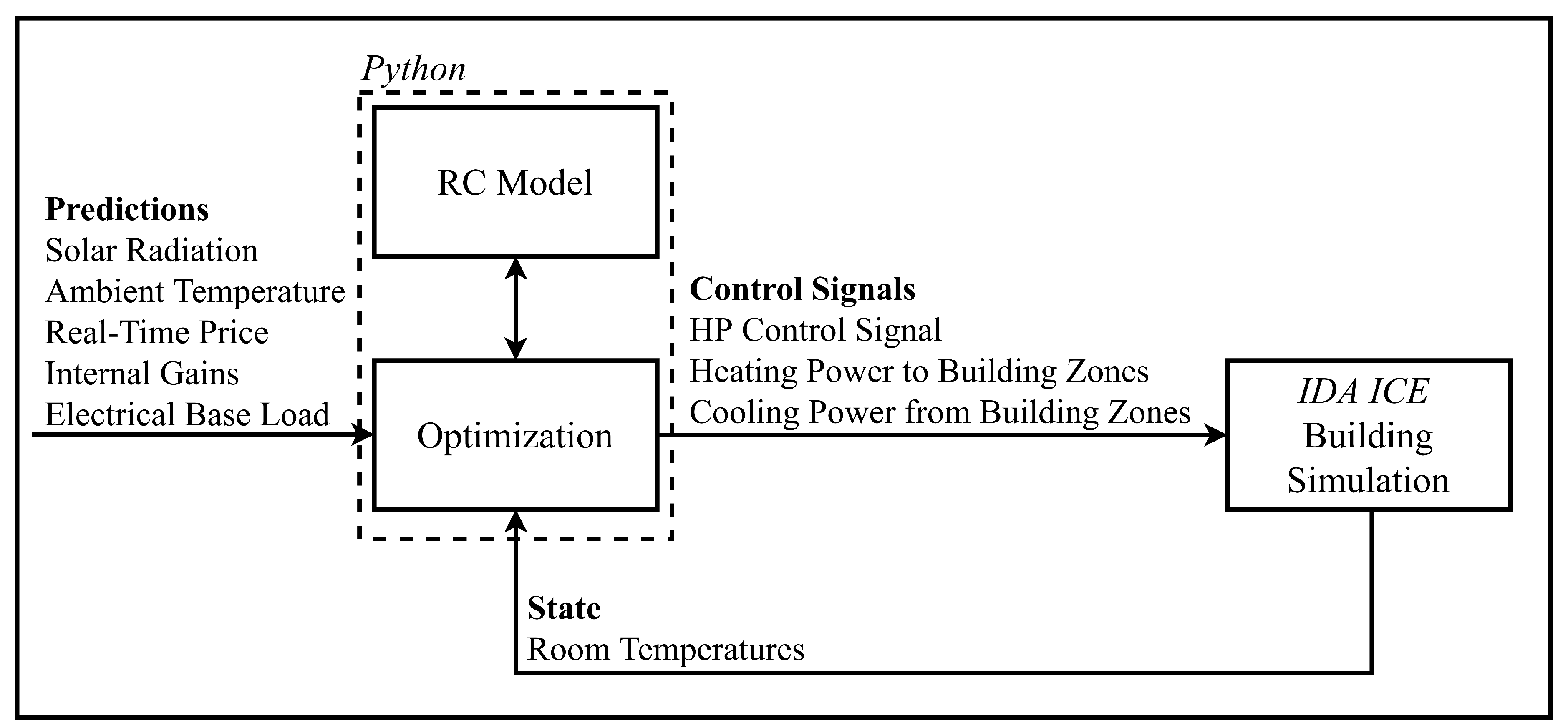
Figure 2.
An aerial view of the real-life NZEB featuring a south-facing PV system on the roof [38].
Figure 2.
An aerial view of the real-life NZEB featuring a south-facing PV system on the roof [38].
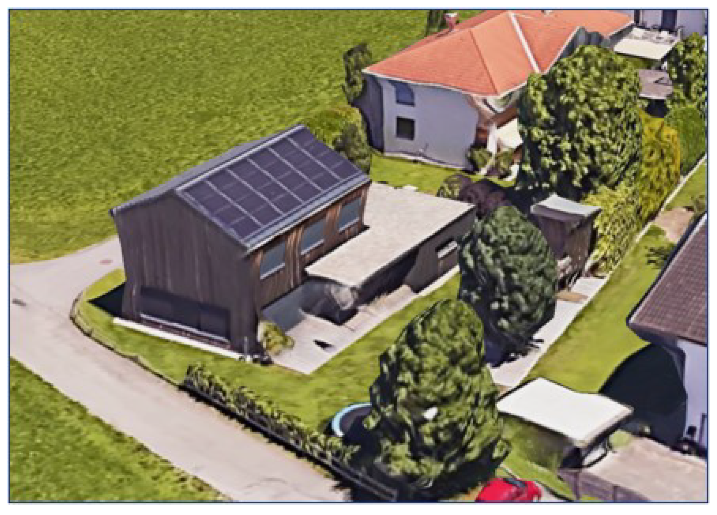
Figure 3.
An aerial view of the IDA ICE NZEB model.
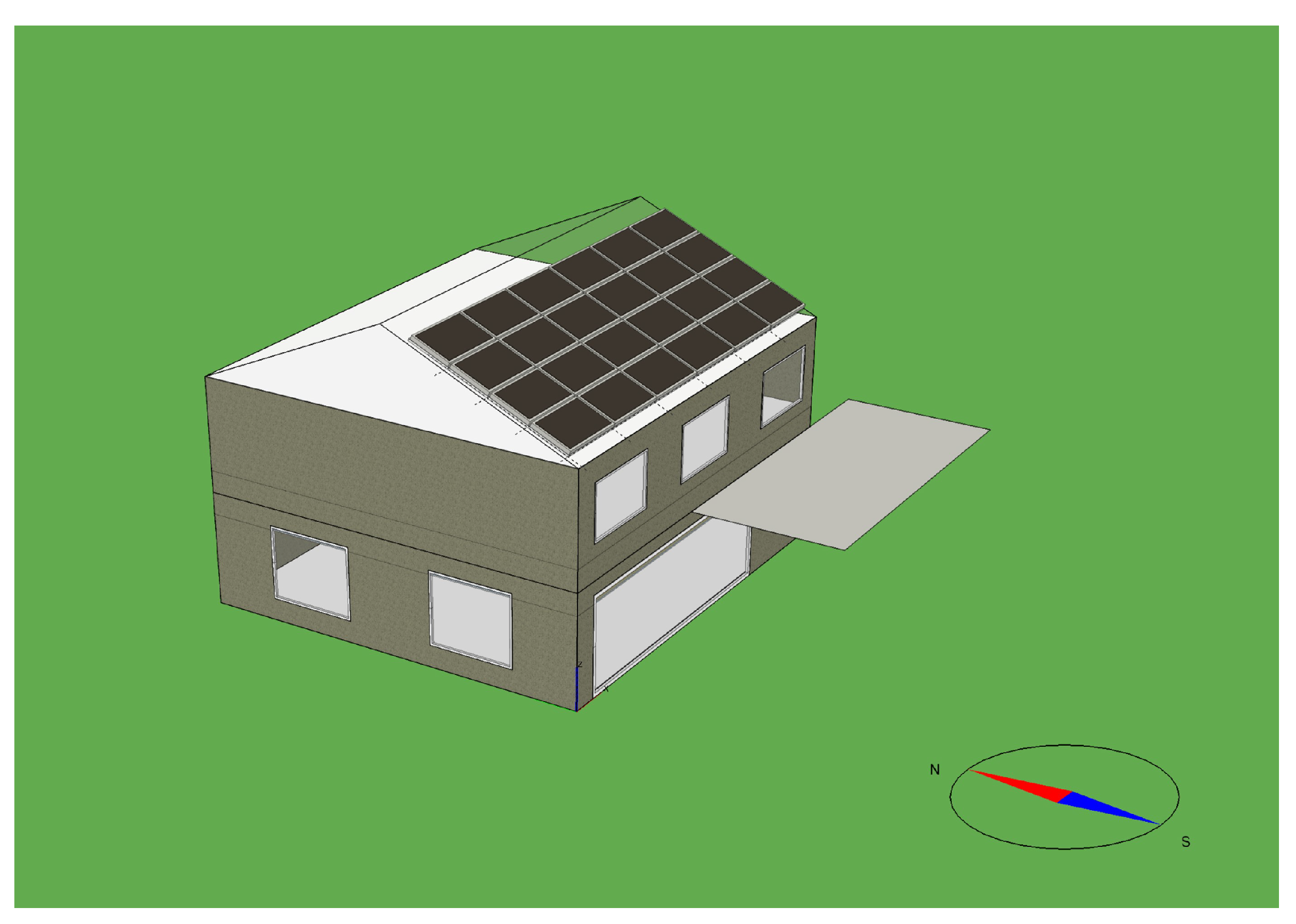
Figure 4.
Reversible heat pump system with heating and cooling circuits, ground-source boreholes including their flow directions.
Figure 4.
Reversible heat pump system with heating and cooling circuits, ground-source boreholes including their flow directions.
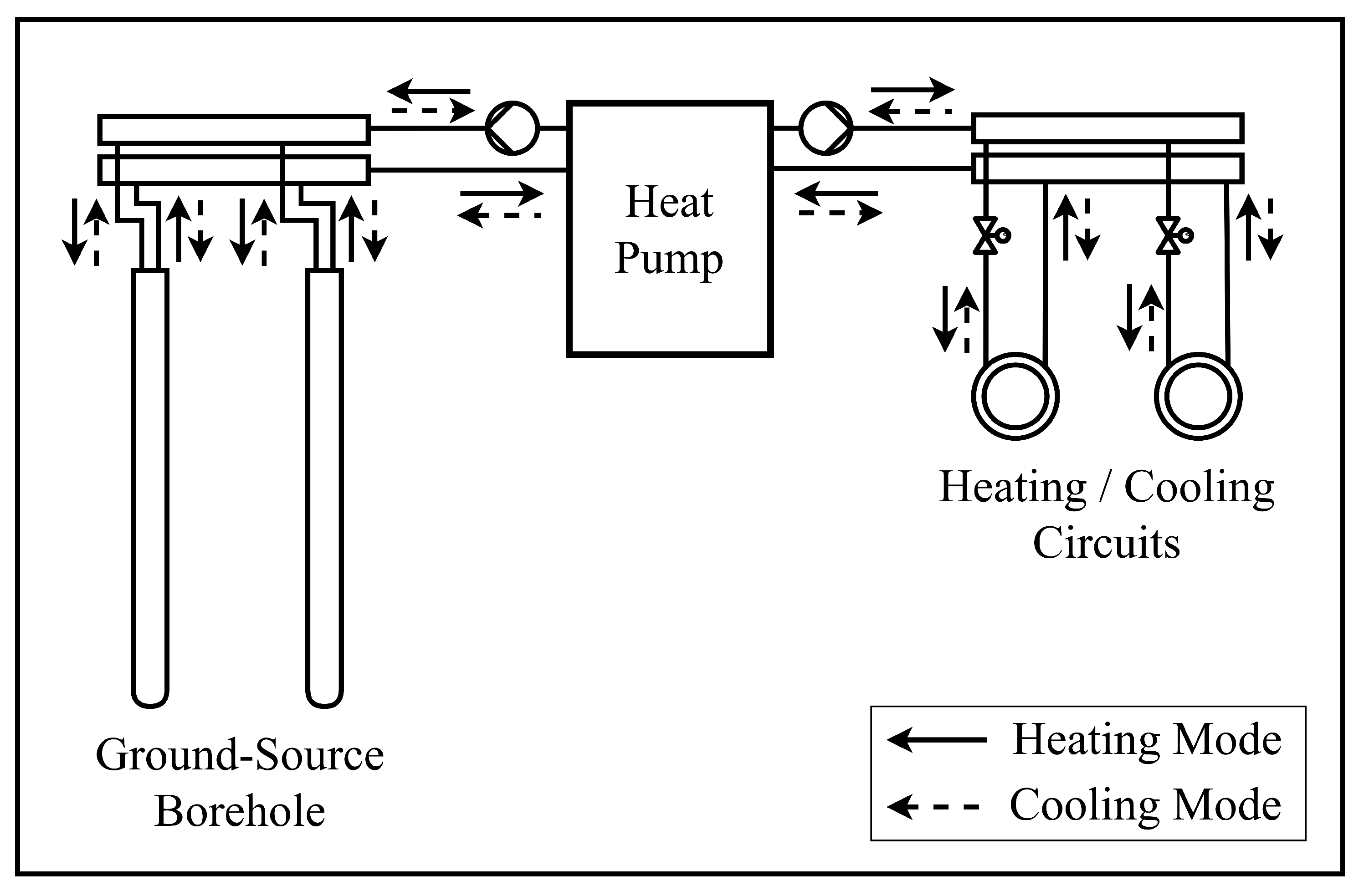
Figure 5.
Thermal RC model of the building including temperature nodes and capacities of the zones and envelope, thermal resistances, and heat flows with thermal gains and losses.
Figure 5.
Thermal RC model of the building including temperature nodes and capacities of the zones and envelope, thermal resistances, and heat flows with thermal gains and losses.
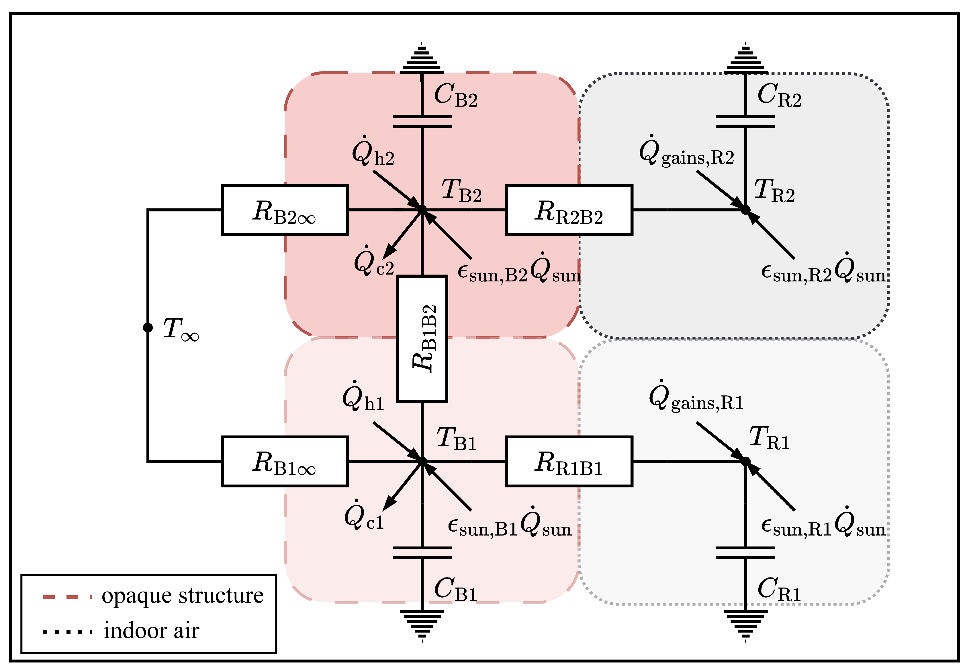
Figure 6.
Overview of the energy produced, used and purchased in the reference case within a year.
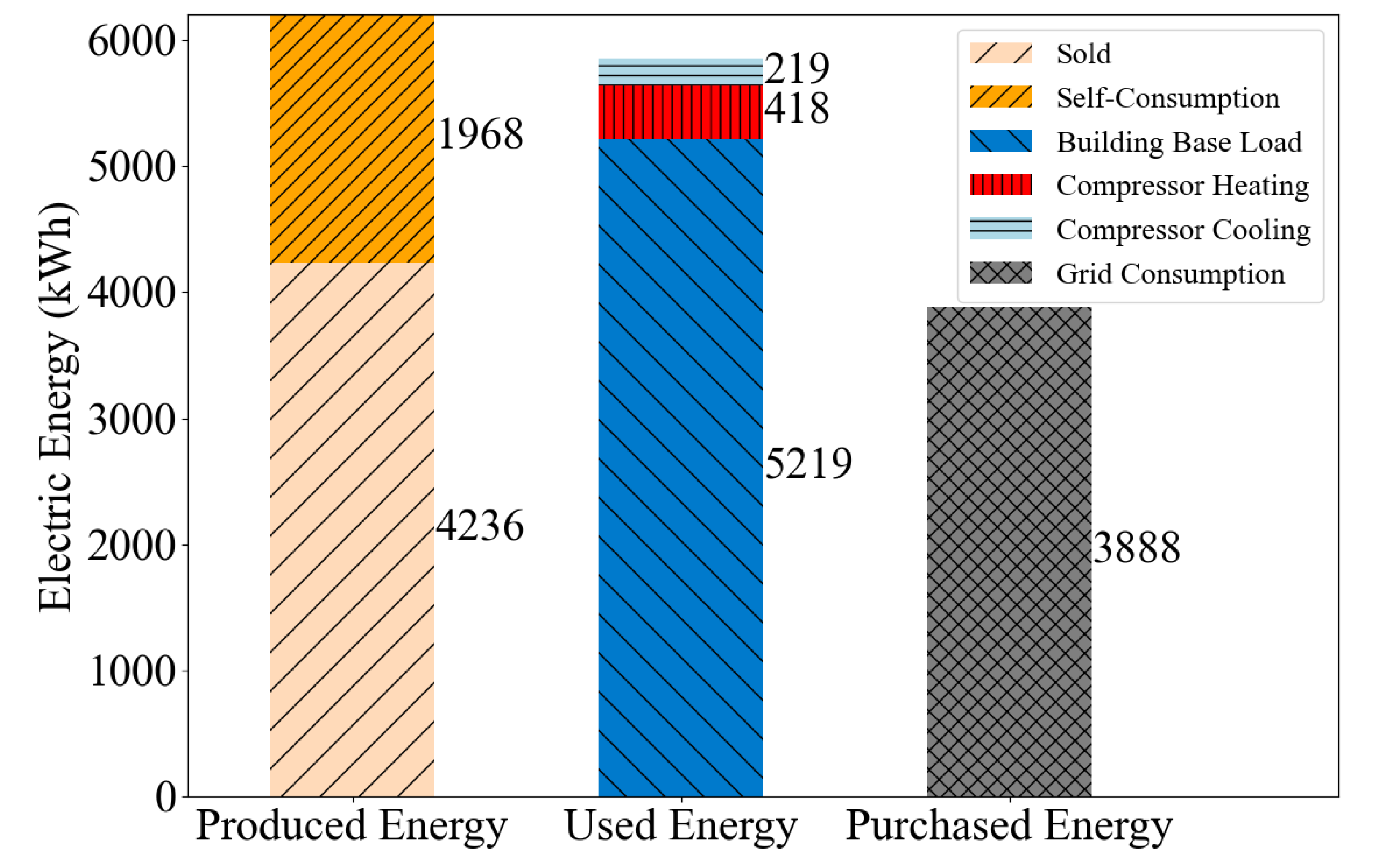
Figure 7.
Comparison of the estimated and simulated room temperatures (left) for room 1 (top) and room 2 (bottom) over a three-day example. Box plots of the estimation errors as squared residuals (right) for one year.
Figure 7.
Comparison of the estimated and simulated room temperatures (left) for room 1 (top) and room 2 (bottom) over a three-day example. Box plots of the estimation errors as squared residuals (right) for one year.
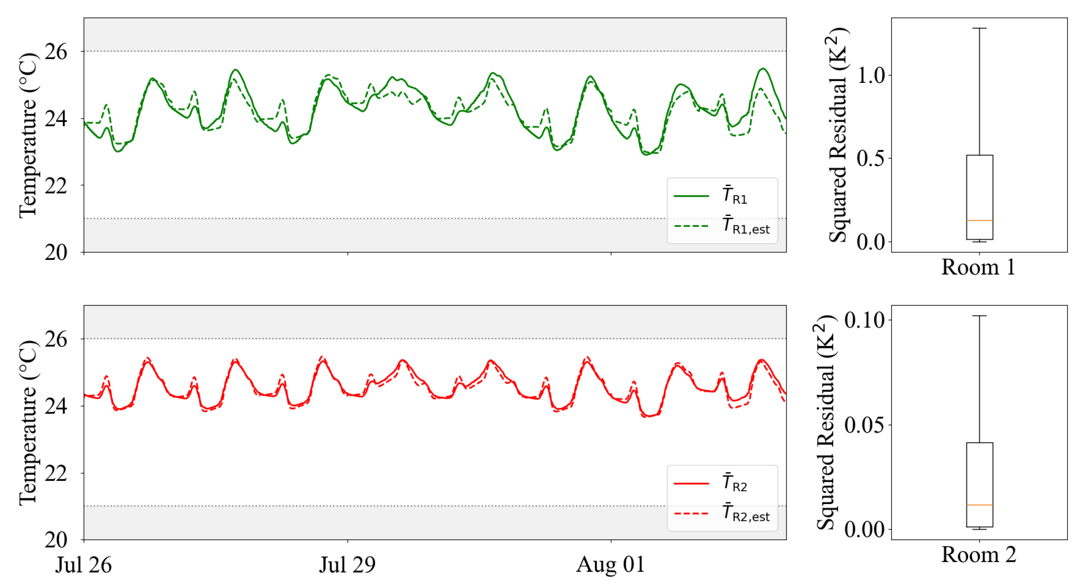
Figure 8.
Optimization results for three example days in summer, where MPC for SC is applied. Subplots from top to bottom represent: comfort criteria via room temperatures, cooling load to zones, produced (PV) and used power (HP and base load), incentive function.
Figure 8.
Optimization results for three example days in summer, where MPC for SC is applied. Subplots from top to bottom represent: comfort criteria via room temperatures, cooling load to zones, produced (PV) and used power (HP and base load), incentive function.
Figure 9.
Comparison of the comfort criteria with Predicted Percentage of Dissatisfied (PPD, top) and Predicted Mean Vote (PMV, bottom) for room 1 and room 2 in the reference case (REF) and MPC for the two scenarios: Real-time price (RTP) and PV self-consumption (SC). Gray-shaded areas indicating negative interference into comfort according to class II of EN 16798-1 [37].
Figure 10.
Highest Exceedance of threshold value for room temperatures (room 1 and 2) and Predicted Percentage of Dissatisfied (PPD) in the one-year simulation of MPC (RTP) for winter (top) and summer (bottom). Gray-shaded areas indicate negative interference into comfort according to class II of EN 16798-1 [37].

Table 1.
NZEB component structures (outside to inside/ bottom to top) with materials, component specifications, orientation, and gross area.
Table 1.
NZEB component structures (outside to inside/ bottom to top) with materials, component specifications, orientation, and gross area.
| Component | Floor/Orientation | Area (m2) | Material | Thickness (m) | tot. U-value (W/(m2 K)) |
|---|---|---|---|---|---|
| Base plate with floor | 1st | 90.0 | concrete + reinforcement (0.25), bituminous sheeting (0.005), leveling screed (0.08), thermal insulation panel (0.16), cement screed + vapor barrier (0.07), flooring (0.015) |
0.58 | 0.16 |
| External wall | 1st / North | 23.3 | timber frame (0.09), wood fiber insulation (0.28), insulated timber frame (0.075), plasterboard (0.015) |
0.46 | 0.10 |
| 1st / West | 16.6 | ||||
| 1st / East | 23.4 | ||||
| 1st / South | 8.8 | ||||
| 2nd / North | 21.8 | ||||
| 2nd / West | 23.4 | ||||
| 2nd / East | 21.1 | ||||
| 2nd / South | 18.2 | ||||
| Windows | 1st / North | 0.7 | insulated glazing | 0.008 | 0.74 |
| 1st / West | 6.8 | ||||
| 1st / East | - | ||||
| 1st / South | 17.2 | ||||
| 2nd / North | 4.2 | ||||
| 2nd / West | - | ||||
| 2nd / East | 2.3 | ||||
| 2nd / South | 7.8 | ||||
| Floor / Ceiling | 1st / 2nd | 90.0 | flooring (0.015), | 0.5 | 0.165 |
| cement screed + vapor | |||||
| barrier (0.07), | |||||
| thermal insulation panel + | |||||
| impact sound insulation (0.115), | |||||
| insulated timber frame with | |||||
| oriented stranded board (0.285), | |||||
| plasterboard (0.015) | |||||
| Roof | 2nd | 92.0 | board stacked ceiling (0.12), | 0.38 | 0.13 |
| wood insulation + | |||||
| vapor barrier (0.24), | |||||
| vapor-permeable wood fiber board (0.016) |
Table 2.
Summary of internal gains per category for each floor (first and second) showing occupancy, equipment, and lighting schedules along with associated power, heat gain, and annual energy values.
Table 2.
Summary of internal gains per category for each floor (first and second) showing occupancy, equipment, and lighting schedules along with associated power, heat gain, and annual energy values.
| Category | Day of week | Schedule (h) | No. of people (-) / Total power (W) |
Activity level (MET) / Avg. Heat gain (W) |
Total energy yearly (kWh) |
|---|---|---|---|---|---|
| Occupancy | Weekdays | 0 [8-15], 0.5 [15-17], 1 otherwise |
2.0 / - | 1.0 / - | - |
| Weekend | 1 [0-24] | ||||
| Equipment | Weekdays | 0 [8-15], 0.5 [15-17], 1 otherwise |
- / 150.0 | - / 114.4 | 1002.0 |
| Weekend | 1 [0-24] | ||||
| Lighting | Daily | 1 [6-8, 15-23], 0 otherwise |
- / 300.0 | - / 125.0 | 1095.0 |
Table 3.
Overview of the RC model parameters identified via the Prediction Error Method (PEM).
| PEM Parameter | Parameter | Value |
|---|---|---|
Table 4.
Aggregated quantities and performance indicators for a one-year simulation of the reference (REF) and the MPC of the two optimization scenarios: Real-time price (RTP) and PV self-consumption (SC).
Table 4.
Aggregated quantities and performance indicators for a one-year simulation of the reference (REF) and the MPC of the two optimization scenarios: Real-time price (RTP) and PV self-consumption (SC).
| REF | RTP | SC | deviation (RTP/SC) | |
|---|---|---|---|---|
| HP operation cost (€) | 82.26 | 47.31 | 46.58 | -42.49% / -43.37% |
| specific HP operation cost (ct/kWh) | 12.91 | 6.73 | 6.56 | -47.91% / -49.26% |
| HP electricity consumption (kWh) | 636.70 | 702.99 | 710.59 | +2.33% / +3.43% |
| HP electricity heating (kWh) | 418.09 | 425.14 | 429.90 | +1.68% / +2.82% |
| HP electricity cooling (kWh) | 218.61 | 277.85 | 280.69 | +27.09% / +28.39% |
| total electricity cost (€) | 722.52 | 687.58 | 686.85 | -4.84% / -4.94% |
| produced PV energy (kWh) | 6204.49 | 6204.49 | 6204.49 | - |
| used energy (kWh) | 5855.27 | 5921.56 | 5929.15 | +1.13% / +1.26% |
| grid consumption (kWh) | 3888.33 | 3717.52 | 3705.71 | -4.39% / -4.69% |
| self-consumption ratio (%) | 31.70 | 35.52 | 35.82 | +3.82%pt. / +4.12%pt. |
| self-sufficiency ratio (%) | 33.59 | 37.22 | 37.50 | +3.63%pt. / +3.91%pt. |
| max. PPD (%) | 15.08 | 19.14 | 18.34 | - |
| avg. PPD (%) | 7.18 | 5.90 | 5.92 | - |
| heating demand (kWh/m2a) | 9.29 | 9.45 | 9.55 | +1.68% / +2.82% |
| cooling demand (kWh/m2a) | 4.86 | 6.17 | 6.24 | +27.09% / +28.39% |
Disclaimer/Publisher’s Note: The statements, opinions and data contained in all publications are solely those of the individual author(s) and contributor(s) and not of MDPI and/or the editor(s). MDPI and/or the editor(s) disclaim responsibility for any injury to people or property resulting from any ideas, methods, instructions or products referred to in the content. |
© 2024 by the authors. Licensee MDPI, Basel, Switzerland. This article is an open access article distributed under the terms and conditions of the Creative Commons Attribution (CC BY) license (http://creativecommons.org/licenses/by/4.0/).
Copyright: This open access article is published under a Creative Commons CC BY 4.0 license, which permit the free download, distribution, and reuse, provided that the author and preprint are cited in any reuse.


