
Submitted:
01 December 2024
Posted:
02 December 2024
You are already at the latest version
Abstract
This paper presents the findings from the initial phases of the SIF BLADE project, focused on demonstrating the capabilities of an offshore wind power plant (OWPP) for power system restoration (PSR). It provides an overview of PSR, highlighting its challenges and operational requirements, alongside the various scenarios considered in the project. The study includes a steady-state analysis to assess whether the OWPP can meet local network demands for both active and reactive power. Results indicate that the OWPP can operate within an envelope that covers all local power requirements. Additionally, EMT analysis were conducted to evaluate different percentages of grid-forming (GFM) converter penetration during the energization process. These analyses aimed to determine compliance with Transmission System Operator (TSO) requirements. Findings demonstrate that all GFM penetration levels met the necessary TSO standards. Furthermore, a novel small signal analysis was performed to identify the optimal percentage of GFM converters for enhancing system stability during block loading. The analysis suggests that for top-up scenarios, a GFM penetration between 20% to 40% is optimal, while for anchor scenarios, 40% to 60% GFM penetration enhances stability and robustness.
Keywords:
Black Start
; Converter Control
; EMT analysis
; Grid-Following
; Grid-Forming
; Power System Restoration
; Small Signal Analysis
; Stability
1. Introduction
Wind energy is becoming a prominent player in the global energy mix, and this trend is expected to continue. One of the main drivers is the need for decarbonization to achieve carbon neutrality, as stipulated in the Paris Agreement of 2015. The European Union aims for 32% of its electricity mix to come from renewable energy sources (RES) by 2030. As of 2020, this percentage was 19.7%, with 16.9% of this electricity produced by wind turbines (WT) [1]. In the UK, 24.8% of the electricity mix came from wind energy, with 11% generated by offshore wind power plants (OWPP) [2]. This unprecedented change in the electrical system has resulted from the decommissioning of fossil fuel-based generators and their replacement with inverter-based RES.
With the increasing integration of converter-connected RES into power grids, it is essential to ensure the resilience of power systems in the event of partial or total blackouts. Traditionally, the responsibility for restoring power, known as power system restoration (PSR) or black start (BS), has rested with a few large, transmission-connected synchronous generating power stations. However, as these stations are phased out, the task of providing restoration services must also transition accordingly, thus RES such as OWPP, photovoltaics (PV), and battery energy storage systems (BESS) should also be considered as black start units (BSUs) [3,4]. BSUs are generation assets capable of restarting without support from the electrical grid. In particular, PSR using wind power has not previously been seen as a priority, but due to the high number of planned OWPP, 50 GW by 2030 [5], it is a matter of energy security to consider this option for the future of PSR in the UK.
Having this in mind, several projects emerged in the UK and European Union aiming research involving both industry and academia in which it was investigated if RES can potentially contribute to UK’s PSR in case of a blackout. An example of such is project PROMOTioN, a project in meshed HVDC offshore transmission networks, investigated OWPP/WT control for self-start and BS [6,7]; another is Distributed ReStart which explored how distributed energy resources (DER) such as solar, wind and hydro, may be used for PSR [8].
Following this trend, the project SIF BLADE [9] was launched, aiming to explore and demonstrate how innovative, cost-effective, low-carbon technologies can enable OWPP to restore the onshore grid following a blackout. Validating this concept will facilitate the accelerated deployment of OWPP to replace existing fossil fuel generators, while mitigating any potential resilience challenges that may arise. This paper aims to present the key topics discussed and analyzed during the initial stages of the SIF BLADE project: the Discovery Phase and the Alpha Phase. Below, the studies conducted during these phases are detailed, along with the sections where each topic is discussed.
Section 2 presents various studies conducted during the Discovery Phase of the SIF BLADE Project. These studies included an overview of the PSR process; PSR requirements and challenges are examined in the context of OWPP; and an investigation into possible scenarios involving the location of the auxiliary power supply (APS) unit responsible for starting up the OWPP and the need for self-start, grid forming (GFM) WT.
Section 3, Section 4, Section 5 and Section 6 present results from the Alpha Phase of the SIF BLADE project. Section 3 introduces the hardware model and converter control strategies used in the study. The hardware model was designed taking into account information from several partners of the SIF BLADE project, as well as a benchmark OWPP suggested in CIGRE documentation. With regards to converter control strategies, two were used, a grid following (GFL) and a GFM one.
Section 4 examines whether the designed OWPP and power system could meet, in steady state, local network demand in terms of active and reactive power operating points, using data from a project partner. This was done via power flow analysis after developing an impedance model and its Thevenin equivalent.
The next two studies examine the need for, and benefits of, including GFM converter controllers in the PSR process. These studies were done for both “anchor” and “top-up” generation possibilities. These two terms have been added to the Grid Code legal text (GC0156) to clarify the roles of different parties involved in restoration services, based on how actively they participate in the restoration process [10]. The anchor generation assumes the role of system energization, effectively having an active role in rebuilding the skeleton network and block loading whereas the top-up generation scenario only accounts for its block loading capabilities, hence just providing active and reactive power as required.
Section 5 delves into electromagnetic transient (EMT) simulations, while Section 6 focuses on linear time-invariant (LTI) studies, via small signal model (SSM). The EMT analysis aimed to analyse if there is an optimal percentage of GFM penetration to meet transmission system operator (TSO) requirements, mitigate potential challenges, and maintain stable operation during PSR. The novelty of this research lies in the LTI studies, which involved a stability analysis via SSM — a study not yet performed in the context of PSR. This study aimed to determine the best percentage of GFM penetration for enhanced stability and robustness of the power system in scenarios involving anchor and top-up generation during block loading.
2. Power System Restoration from Offshore Wind Power Plants—An Overview
PSR is a complex process with low probability but high impact [11]. This section provides an overview of the PSR process, highlighting its challenges identified by both academia and industry. Additionally, the requirements for PSR are discussed. Finally, the section presents the scenarios studied in this project concerning the location of the auxiliary power supply that will provide the energy required to start-up the OWPP.
2.1. PSR Process
PSR is the ability to restore a power system to its normal state after a partial or total blackout, ideally with minimum losses and restoration time, thereby minimizing economic and social impacts [12]. Traditionally speaking, the stages of power system restoration are split into three different areas, which are BS, network reconfiguration, and load restoration [13,14,15].
The BS stage is characterised by a BSU providing cranking power to a non black start unit (NBSU), hence energizing units that are not self-start capable [15]. This phase also involves identifying the affected power system, including the location of critical loads, the status of circuit breakers, and the availability and location of BSU [3,16,17]. Entities such as the TSO will then choose BSU to restart the system, considering factors such as cost reduction, restoration time, and paths. In the case of OWPP, if multiple are BSU and wind forecasts are favorable, different units will contribute to system restoration, thus, the system is split into generating islands that will later be synchronized [1,2,15].
After a BSU establishes an energized path and supplies the cranking power to a NBSU, the generation capacity increases. The focus of network reconfiguration is on restoring additional generators, constructing the skeleton network that includes key substations and branches, and preparing the system for the final stage of PSR. To accomplish this, the network reconfiguration stage must follow an optimized restoration procedure to ensure a successful restoration and minimize the risk of system re-collapse. According to [3,4,5,13], this procedure includes enhancing the grid resilience by including temporary backup power, emergency power supplies, topology reconfiguration, substation relocation and transmission line rerouting.
During the BS phase, a BSU unit is employed to energize the electrical path and supply power to a NBSU. This stage focuses on restoring enough load to enable the BSU unit to achieve its minimum operational output. As the process transitions to the network reconfiguration stage, increased generation capacity allows for the restoration of additional loads, helping to balance the load and generation levels [14]. This stage also provides the opportunity to restore critical loads. Prior to the third stage, load pickup primarily serves to manage system frequency. In contrast, the third stage is dedicated to restore as quickly as possible the rest of the loads connected in the system [17,18].
Aforementioned is the traditional set up for PSR. Nevertheless, this approach may also be followed if considering system restoration from RES, more specifically, from OWPP. However, due to the new technologies implemented in OWPP such as inverter-based generators, some challenges and concerns will be distinct.
OWPP have the potential to provide PSR due to their large capacity and the increasing sophistication of their technology. The process begins with the self-start capability of the OWPP, which can be facilitated by cranking the WT via an external power supply such as a BESS or GFM WT. It should be mentioned however, that the GFM technology is new and thus immature, and presents several technology complexities. Furthermore, GFM WT may come with extra costs that should be considered. These systems can establish an initial power island by energizing part of the OWPP independently of the main transmission network [19]. Once the initial power island is established, the OWPP can progressively energize larger sections of the grid through a method known as block loading. This involves sequentially connecting and energizing sections of the transmission network until the entire system is fully restored. During this phase, the OWPP must maintain voltage and frequency control to ensure stability and prevent overloading [20]. A critical aspect of the restoration process is the synchronization of the OWPP with other energized sections of the grid. This requires control and coordination to match the phase and frequency of the local grid with the larger transmission network [20,21]. Once synchronized, the OWPP can contribute to the overall stability and resiliency of the power system, providing a renewable-based alternative to conventional black start sources.
2.2. Challenges and Requirements of PSR from OWPP
The European Network of Transmission System Operators (ENTSO-E) included BS and island operation as optional requirements for AC and HVDC connected OWPP. However, there are currently no PSR requirements specifically dedicated for OWPP [20]. However, several TSOs, such as Elia from Belgium, and National Grid ESO (NGESO), from the United Kingdom, have proposed a set of requirements [8,10,22]. This section describes succinctly some of those requirements that shall be used later in Section 5 for the EMT studies. It also dives into challenges identified for PSR from OWPP. For further details on all the requirements, readers are encouraged to consult references [8,10,20,21,22] as several requirements such as trip to household, time to connect and service availability are not considered in this study.
2.2.1. Self-Start Capability
A BSU needs to be able to self-start without any external power supply within a specific time frame which is dependent on the TSO. Traditional WT are not self-start capable as they are GFL units, thus, follow a voltage reference signal from another voltage source. However, GFM units, if allied with a APS such as an internal BESS or an external APS available to provided cranking power, are able to sustain a voltage reference signal and are thus self-start capable.
2.2.2. Block Loading Capability
Block loading capability refers to a BSU ability to accept an instantaneous block load. The specific value depends on the TSO. As noted in [8], the preferred range for this value is between 35 to 50 MW, while maintaining voltage and frequency within acceptable limits. The document suggests that block loading should be determined by the voltage level at which the BSU is operating. For 400/275 kV and 132 kV systems, the range remains 35-50 MW; for 33 kV systems, the recommended range is 10-20 MW; and for 11 kV systems, it is 0.4-1 MW.
2.2.3. Frequency and Voltage Control
This pertains to maintaining frequency and voltage within acceptable limits during block loading. The frequency must remain between 47.5 and 52 Hz. According to NGESO, the voltage should stay within 10% of its nominal value, while Elia specifies voltage limits based on the block loading conditions [20].
2.2.4. Reactive Capability
NGESO mandates that wind farms possess a reactive power capability of 50 MVar, while conventional generators are required to provide 100 MVar. Conversely, Elia sets different reactive power requirements for various BS zones, with standards in Belgium typically ranging from 30 to 50 MVar at the low-voltage side of the step-up transformer. Shunt reactors can assist in meeting these reactive power needs [20,21]. Long cables operating under low load conditions can generate substantial amounts of capacitive reactive power, which the BS unit must absorb. Reactive capability involves not only the ability to energize the transmission network without active power (reactive power at zero crossing) but also the management of magnetic inrush and transient voltages during energization.
2.3. Scenarios to Energize OWPP
In this section, different scenarios for energizing an OWPP are discussed. A BSU needs to self-energize and contribute to network reconfiguration. Traditionally, such unit uses a small cranking generator, such as a DG, for this purpose. For OWPP, an APS like a synchronous DG or a BESS can be used to start wind turbines. Alternatively, GFM WT can self-start. The size of the cranking unit needs to have enough energy to start key components that enable power generation. These include the wind turbine controllers and communications, heating and cooling loads, water and oil pumps, and motors such as the pitch and yaw. According to [23], the auxiliary power needed to self-start a wind turbine is less than 5% of its rated power.
The SIF Blade project explored four energization solutions, with two selected for further study. These solutions vary based on the APS location and the requirement for GFM WT. An APS, if located onshore or offshore, can provide a stable voltage reference, eliminating the need for GFM WT as all GFL WT will synchronize with the APS voltage. Self-starting wind turbines must be GFM capable. The four scenarios considered in this study to energize the OWPP may be seen in Table 1.
Figure 1 graphically illustrates the locations of S1, S2, and S3; S4 is a combination of these APS. In the figure, S1 is situated in the onshore substation, along with several loads, the local network, and a variable shunt compensation. S2 represents an APS located inside a WT, indicating a self-starting WT. S3 is positioned in the offshore substation, following the offshore transformer and static shunt reactive compensation, but before the HVAC export submarine cable.
Scenario 1 (S1) involves placing the APS at an onshore substation. The APS would need to energize all equipment from the substation to the OWPP, including the substation itself, reactive power shunt compensations, offshore submarine HVAC export cable, OWPP array cables, and finally the wind turbines. Although this process requires significant energy, the onshore location of the APS allows for larger units due to space availability, unlike offshore substations or wind turbines. Additionally, APS units are typically already available at or near onshore substations. Scenario 1 is thus an attractive solution due to its simplicity and technology readiness. Located onshore, the APS is easier to install, operate, and maintain, with no space limitations. It can keep a stable voltage reference signal, eliminating the need for GFM wind turbines.
Scenario 2 (S2) considers self-starting wind turbines which have the capability to energize themselves. This is done via an uninterruptible power supply (UPS), a small BESS or diesel generator inside a wind turbine. Such wind turbines would need to be equipped with grid forming converter control technology as to be able to keep a constant and reliable voltage source reference signal. Once one, or several self-start, GFM, wind turbines are energised, these units would be responsible for providing enough energy to energise the OWPP array cables and the GFL wind turbines, which would then synchronise with the GFM units.
Previous studies have explored the concept of self-start wind turbines for OWPP. In [24], a method is proposed where wind turbines start using their internal energy storage without external generators. In [25] it is discussed an autonomous startup and synchronization using the wind turbine APS to sequentially energize turbines. Additionally, in [26] is introduced a wind turbine equipped with a DG that can generate power during a blackout, replicating the electricity network and supporting auxiliary devices.
In Scenario 3 (S3), an APS is located in the offshore substation. Firstly the offshore transformer and substation equipment are energized and then the OWPP itself, reducing energization time compared to an onshore APS. The offshore industry, particularly the oil and gas sector, is familiar with APS in offshore substations, and Battery Energy Storage Systems (BESS) are a topic of interest for such platforms [27,28,29,30,31]. However, limited space in offshore substations makes it challenging to include a BESS unit solely for black-start purposes if the OWPP is already constructed. Scenario 3 is the most expensive due to higher installation and maintenance costs and limited accessibility. Although grid-forming wind turbines are recommended, they are not necessary as the APS can generate frequency and voltage. Some offshore substations may already have an APS capable of cranking the first wind turbine, providing an alternative for auxiliary power.
Scenario 4 (S4) proposes a hybrid solution combining onshore and offshore auxiliary power supplies. For example, an onshore BESS could work alongside GFM self-start wind turbines or an additional offshore BESS. This approach reduces costs and improves accessibility compared to other scenarios, while also increasing available energy and redundancy. Some studies already mention this alternative [32,33,34]. This hybrid configuration leverages the advantages of both onshore and offshore setups, ensuring a more flexible energization process for the OWPP.
For this project, Scenarios 1 and 2 were selected based on their advantages. Scenario 1 was chosen primarily due to the existing readiness of technology and the availability of onshore APS units for future tests. An onshore APS not only facilitates the energization of the OWPP but also provides additional benefits such as voltage and frequency regulation if necessary. Further, since this unit is bigger, it might be able to sustain a voltage reference signal for longer. Scenario 2 was selected due to the project’s high level of expertise and the interest from various partners in utilizing self-starting, GFM wind turbines. This scenario is cost-effective and offers a shorter restoration time, making it a practical choice for efficient and rapid energization. In this paper, for both EMT and SSM analysis, only scenario 2 was considered.
3. System Under Study
In this section it is introduced the hardware and the converter control strategies used throughout this study. The hardware will vary according to each section, however, those changes will be explained in the section itself. Thus, a baseline of the hardware analysed is given.
3.1. System Modelling
Figure 1, introduced previously, shows a one-line diagram of the model used throughout this paper, although, for each section, some changes will be done to this model. The diagram illustrates a system containing an OWPP with a BESS and a self-starting, grid-forming wind turbine. In the figure, the OWPP connects to the power system via an offshore transformer, which steps up the voltage from 66 kV to 230 kV, the voltage of the submarine export HVAC cable with a length of 50 km. The latter benefits from two shunt reactor compensations: a static one located offshore at the beginning of the cable (included in the offshore substation for practical purposes) and a variable one in the onshore substation. These compensations address the high capacitance of the submarine cables.
The system also includes an onshore transformer, which steps up the voltage from 230 kV to 400 kV and a local network, operating at 400 kV. This local network, displayed after BRK5, was considered for a specific purpose. The OWPP can be used as a top-up or anchor BSU generator. The top-up scenario means the OWPP will only contribute as an active and reactive power provider, whereas the anchor generator actively helps in the process of network reconfiguration and block loading.
The designed hardware system further includes several loads represented as impedances after BRK7 and BRK8 which are used to test if the OWPP can provide the required active and reactive power to the local network.
Further, the breakers seen in the figure are included to test the energization process, study possible transients (especially during transformer energization, cable and shunt reactors energization), thus test if the EMT simulations meet the TSO technical requirements specified earlier.
As the hardware system will vary according to the study that will be presented, the parameters utilized are described in each section.
3.2. Converter Control Strategies
Two converter control units were used in this study, a GFM and GFL one. This section describes both, which may be seen in Figure 2. Further, the parameters of the controllers used in this study may be seen in Appendix A, Table A4 and Table A5 for both grid-forming and grid-following controllers respectively. Further, a supervisory frequency controller was designed and is also explained in this section.
3.2.1. Grid Forming Unit
The GFM unit used in this study is called VSM and is based on the studies described in [35,36,37,38]. Such name was given as it emulates through its controllers the behaviour of a synchronous machine. A diagram of such may be seen on the right side of Figure 2. It consists of two PI controllers: one is referred as the power loop (P/f loop) and the other the voltage loop (Q/V loop). Further, a virtual impedance was added to this controller due to the transients that may happen throughout the energisation process of the power system.
The power PI controller computes the angle of the point of common coupling (PCC). The voltage PI controller computes the component of the voltage to be fed to the converter and the component is zero. Thus, the Clark transformation is used instead of the Park Transformation.
From the figure, the power PI controller is defined as shown in Equation (1).
where is the proportional gain and the integral gain of the power controller. With regards to the voltage controller, the PI is defined as follows
where is the proportional term and the integral term.
Several studies were analyzed with regards to virtual impedance implementation [39,40,41,42,43,44] and eventually the approach described by Rodriguez-Cabero et. all described in [43] was followed. The virtual impedance is located after the PI voltage controller. Thus, the q component of the voltage which is fed back to the converter, , is given by
where is the voltage reference of the controller, is the q component of the voltage at the PCC of the grid forming converter and and are the synchronous reference frame components of the current measured at the converter terminals. For the d component of the voltage at the converter terminals, is given by
3.2.2. Grid Following Unit
The grid following controller here used is called Standard Vector Current Controller (SVCC) and it was based on the one that may be found in [45]. A scheme of such may be seen in the left side of Figure 2. It consists of a PLL, a current inner loop and voltage and power outer loops. The PLL has the objective of computing the angular velocity of the electrical network. To do so, a PI controller is implemented as displayed in Equation (5).
where is the integral gain and the proportional term . The inner loop is the lower-level control of this GFL unit. It allows the independent control of both q and d components due to its decoupling terms. The output of this controller is the voltage which is fed back to the converter. The control of both components in the synchronous frame is done via PI controller as shown in Equation (6).
where is the integral gain and the proportional term is . The outer loop controller computes the current references in the synchronous frame and which are later fed into the inner loop controller. This is done considering the active power and voltage magnitude of the system. Both voltage and power outer loops are also controlled with PI controllers as shown in expressions 7 and 8 respectively.
where and are the proportional gains of both power and volage outer loop controllers and and are the integral gains.
3.2.3. Supervisory Frequency Support Controller
Standard GFL wind turbines often face frequency stability problems and typically lack droop control [46]. When restoring the power system, various voltage and frequency disturbances can occur, which the standard GFL controller, shown in Figure 2, does not address. To manage these issues without altering the existing controller structures, an external supervisory controller was developed to help prevent frequency drops during load restoration.
This external controller provides frequency support, similar to how a governor functions in a synchronous generator. It uses a PI controller integrated with both GFM and GFL loops. The controller adjusts the active power references in both GFM and GFL systems to keep the frequency within acceptable limits set by the TSO. The power adjustment is shared between the GFM and GFL controllers based on the level of GFM penetration, as shown in Figure 3. The controller reacts to frequency deviations () by distributing a power increment ( and of ) between the GFM and GFL controllers.
4. Steady State (P,Q) Operating Points
The aim of this study was to assess if the offshore wind power plant connected to the power system introduced before could generate, in steady state, an envelope of active and reactive power (P,Q) operating points that would encapsulate the local network (P,Q) needs, thereby matching local network demand. The network demand was provided in terms of (P,Q) operating points, for different wind speeds, demands and paths in the UK.
To examine the steady-state operating conditions, a power flow analysis was conducted. Firstly, the hardware model described in Section 3 was simplified to achieve an impedance model, facilitating the utilization of a Thevenin equivalent for the purpose. Subsequently, the local network demand data was assessed. Once this step was completed, the voltage magnitude and angle of the OWPP were varied to delineate its operational envelope and understand if it effectively encapsulated the operation points of the local network. This iterative process was carried for various conditions, changing the wind speed and local network demand.
4.1. Impedance Model and Thevenin Equivalent
The hardware model shown in Figure 1 was simplified using passive components for this study, as may be seen in Figure 4. This simplification was done to enable a power flow analysis via Thevenin equivalent impedance. In this figure, an aggregated offshore wind farm is represented with a voltage source E and its LC filter via and . The offshore transformer is represented by and . The model also includes offshore shunt compensation with and , and onshore shunt compensation with and . The export cable is modeled as a cable with parameters , , and . Additionally, the grid line is represented with parameters and and is connected to a load, .
The system represented in Figure 4 was further simplified in impedances as may be seen in Figure 5. This way, the entire system was encapsulated, only considering a voltage source with varying magnitude, , and angle, , an equivalent impedance, representing all the system components, and the load. This way it was possible to vary the impedance depending on the system parameters such as OWPP nominal power output, local network demand and wind speed and analyse the impacts on the load, which here represents the local network demand, as will be explained in the next section.
From Figure 5, the final Thevenin voltage and impedance are given by
where is the Thévenin voltage and the Thévenin impedance. Such impedance will be later used having its real part, R, and imaginary one, X, separated.
Considering the Thévenin equivalent described by Equations (9) and (10), the current flowing through the converter is
The apparent power, S, at the converter terminals is
Developing this equation and separating the real and imaginary parts, the active and reactive power flow equations for the power converter are achieved.
4.2. Local Network Loads
As per stated in the grid codes of the UK regarding power system restoration, dispatched providers all together need to be able to restore 60% of the network demand in the first 24 hours and 100% in 72 hours. This energization is done in steps of active and reactive power. Depending on several conditions such as number of generators available, demand and wind speed conditions, black start generators will be chosen to be part of the energization process, be that of network reconfiguration or block loading.
The data here considered to study the capabilities of an OWPP to meet local network demand is based on real data provided by a party of the SIF Blade project. It is assumed that a local substation demands active and reactive power in steps to energize several loads. This energization process is depicted in Figure 6 for three different cases where demand, energization path and wind speed varies. These are the three load demand cases that shall be studied in the this section.
4.3. Case Studies
In a controlled OWPP, the voltage magnitude and angle output are regulated by the action of the converter controller. However, in this case where the interest was to compute operating points via power flow, the model shown in Section 4.1 was utilized and the operating points of the system computed using the previous Equations (13) and (14).
For each case introduced previously in Section 4.2, the output voltage and angle at the terminals of the converter were varied to create the operating region of the OWPP. The wind speed used in this analysis was given by a SIF Blade project party. This quantity was varied between 0 and 1, where 1 would mean rated wind speed and 0 no active power production. Hence, to compute the active and reactive power available, the apparent power was multiplied by the wind speed ratio.
Table 1 displays the wind speed used for each case, the converter terminals angle and voltage magnitude that were needed to generate the OWPP envelope. Figure 7 displays the results of such envelope for the three study cases. Results have shown that the OWPP connected to the power system considered was able to create an area of operation capable of enveloping the local network demand for three different study cases where the wind speed and demand changed the active and reactive power operating points in the local network.

Table 2.
Wind speed, converter voltage angle and magnitude for the different study cases.
| Case | Wind (%) | (pu) | |
|---|---|---|---|
| 1 | 0.15 | -5 to 2 | 0.95 to 1.02 |
| 2 | 0.6 | -10 to 3 | 0.91 to 1.01 |
| 3 | 0.35 | -8 to 2 | 0.93 to 1.02 |
This was achieved without varying any parameter in the impedance model, as introduced in Equations (9) and (10). Thus, there is margin to vary even further the converter terminal voltage magnitude and angle to accommodate local network demand, as well as potentially increase or decrease the shunt compensation that exists in the model. Further, the study here presented was performed for a cable length of 50 km, hence the impact of the capacitance of the HVAC cable did not play a major role in active power losses nor reactive power needs. If such issue arises, and as it was was previously observed in [47], these components significantly impact the voltage stability of the system in steady state as well as the (P,Q) operation envelope which the OWPP may provide to the local network, this study may be carried varying the shunt impedance to analyse how much reactive power would need to be compensated.
5. Grid Forming Penetration - EMT Studies
This section presents the EMT studies conducted to analyze the time domain performance in the PSR process. The aim was to determine if different levels of grid-forming penetration would meet some of the technical requirements set by the TSO. The requirements examined are described in Table 3. In this study, the GFM penetration was varied between 0% to 100% in steps of 20%.
Figure 8 displays a one-line diagram of the model used for the time domain studies and Appendix A contains the parameters that were used in this study. To analyze the optimal grid-forming penetration, the aggregated wind farm was split into two parts, each with a controlled voltage source converter (with voltages and ) and their LC filters (parameters and ), representing both GFM and GFL converter penetrations. This setup allowed for varying the percentage of GFM penetration.
The model further includes an offshore transformer that steps up the voltage from 66 kV to 230 kV. An HVAC export cable is represented using a equivalent model with parameters , , and . This cable has a length of 50 km. Due to the high capacitance of submarine cables, two shunt reactive power compensations were included: one fixed offshore ( and ) and one variable onshore ( and ). Four RC loads were connected to simulate the block loading capabilities. The active and reactive power steps and respective values of and may be seen in Table A2 of Appendix A.
Additionally, the scenario tested here is scenario 2, involving self-starting wind turbines, with a BESS connected via breaker BRKB to the upper branch of the OWPP. Although the BESS may have several purposes, in this study, it was only used for wind farm energization. It should also be noted that an aggregated wind farm model was used in this study, so array cables of the wind farm and wind turbine transformers were not considered, but study is considered as future work. Furthermore, only the offshore transmission system was considered as no onshore cables were modelled for this study. Furthermore, both top-up and anchor generation scenarios were used. In case of the top-up scenario, as an external grid is present during the energization process, breaker BRK7 is closed. In case of anchor generation, BRK7 was open through all the simulations and hence, no external grid support was available.
5.1. Energization Sequence
The energization process is detailed in Table 4. It begins by energizing one or several self-start capable WT (depending on the percentage of GFM penetration) by closing breaker BRKB. In this study, all GFM WT are assumed to be self-start capable. Once these units are energized, breaker BRKF is closed to energize the rest of the OWPP, including the GFL units. This step poses synchronization challenges. Since this study involves an aggregated wind farm model, the resulting transients may not accurately represent the actual events and this topic is not discussed here, however, it will be addressed in future research.
After the OWPP is fully energized and operating in islanded mode, breaker BRK1 is closed to energize the offshore transformer. This step presents technical challenges which are addressed in technical requirement number 4, displayed in Table 3. To address this issue, the point on wave (POW) strategy was employed. Several studies discuss the mitigation of inrush currents [48,49,50,51], so this topic will not be fully explored here. However, a brief description of the POW strategy is provided below due to its application in this study.
After energizing the offshore transformer, breaker BRK2 is closed to energize the shunt compensations and the HVAC export cable. It should be noted that in a real-world scenario, these components would likely be energized separately. This step also presents challenges related to transient performance during energization or de-energization processes. These transient phenomena can result in inrush currents, high overvoltages, current zero-miss and transient recovery overvoltages in circuit breakers. These phenomena will depend on the length of the cable, power-frequency voltage, system short-circuit power, shunt compensation and switching instant and may be mitigated applying proper shunt compensation, closing a circuit breaker at a specific time or using a pre-insertion resistor [52,53,54,55,56].
Once the path from the OWPP to the onshore network is fully energized, the process of block loading starts. Subsequently, BRK3, is closed, followed by BRK4, BRK5 and BRK6 to energize the for RC loads representing the active and reactive power demand from the local network. These loads were energized every two seconds.
5.2. Results
This section displays the results of the EMT simulations. For each step of energization, it was seen if the TSO requirements mentioned in Table 3 were met. The section is split as follows: Section 5.2.1 introduces the transformer energization; Section 5.2.2 the shunt reactors and cable energization; Section 5.2.3 displays the results of the block loading for both top-up and anchor scenarios. In Section 5.3, final results are displayed and conclusions drawn.
5.2.1. Transformer Energization
The energization of a transformer may results in inrush currents due to the saturation of its core. Several strategies were studied in academia such as the pre-insertion resistor, point on wave (controlled switching) and sof-start. These may require changes in the converter control strategy or even in the transformer hardware. These strategies are detailed in the following studies [57,58,59,60,61,62,63].
Due to its simplicity, the classic controlled switching strategy (POW) was used in this study. This technique relies on closing the breaker of the offshore transformer at an instant at which the residual flux is equal to the prospective flux, that is, at an optimal closing angle . This may be seen through Equation (15) where the instantaneous flux is calculated [59].
where is the core flux, is the voltage of the energized transformer primary, is the core inductance, is the primary inductance summed with the core inductance, is the primary resistance, is the angular frequency and is the angle at which the breaker is closed and transformer energized. If the residual flux is equal to the prospective flux, the decaying term in Equation (15) is eliminated and thus, the inrush currents neutralized.
The prospective flux can be estimated using Equation (16). This equation shows that the prospective flux is obtained by integrating the voltage applied to the energized (primary) side.
For this study, the parameters of the transformer used may be seen in Table A3. Firstly, a simulation was analyzed without any inrush current mitigation strategy, thus, the breaker was closed at a random instant, of t= 3.3 s. Results of such simulation may be seen in Figure 9. From this figure it is noted that the transformer suffers severe inrush currents, in the order of 10 kA and voltages at both primary and secondary go above and below TSO allowed limits.
Figure 10 displays the results of the offshore transformer energization using the POW energization strategy for a GFM penetration of 20%. For the residual flux considered (that may be seen in Table A3 of 0.8 pu, the optimum instant of closing the breaker was computed at t = 3.2117 s. In this figure, it may be seen that the inrush currents are mitigated, with the maximum inrush current being of 5 A. Both primary and secondary voltages of the transformer are within acceptable TSO limits.
The POW strategy was applied for various percentages of GFM penetration. This strategy effectively mitigated inrush currents in all cases as may be seen in Figure 11.
However, the magnitude of the inrush currents varied slightly depending on the GFM penetration. This variation occurs because, at the computed instant when the breaker is closed, the voltage on the primary side of the transformer differs slightly, leading to slight variations in the prospective flux. Since the optimal breaker closing angle is based solely on the residual flux within the transformer core, the prospective flux and residual flux will not be exactly identical, resulting in slight differences in inrush current magnitudes. Additionally, it was seen that the offshore transformer is energized only after the GFL units are synchronized with the GFM units and the OWPP is running in islanded mode, which can cause some voltage distortions. Allowing time for the waveform to stabilize and return to its natural sinusoidal form before energizing the transformer is necessary; otherwise, undesired inrush currents may occur. Despite these variations, the POW strategy successfully mitigated inrush currents across all levels of GFM penetration, demonstrating its effectiveness regardless of penetration levels.
5.2.2. Shunt Reactors and Export Cable Energization
After energizing the offshore transformer, breaker BRK2 was closed to energize the offshore HVAC submarine cable, along with both offshore and onshore shunt compensations. The offshore reactor is static, while the onshore compensation is variable. This means that the onshore compensation value will adjust based on the reactive power requirements, which might differ for normal operation, energization or de-energization.
As previously mentioned, the submarine cable is 50 km long and produces significant capacitive reactive power. A load flow analysis was conducted to design the shunt compensations to mitigate this reactive power, ensuring that the cable voltage remains within acceptable TSO limits and the power factor stays close to unity at the PCC. It was concluded that 270 MVAr would be compensated via shunt reactors, and 40% of such quantity would come from the offshore reactor and 60% from the onshore one.
To prevent overvoltages and the zero-missing phenomenon, which occur when reactive power compensation exceeds 60% due to interactions between inductive and capacitive components in both the cable and reactors, a Pre-Insertion Resistor (PIR) was implemented. Additionally, incorporating two shunt compensations, rather than just one onshore, was a critical measure to mitigate these phenomena.
The value of the PIR and the optimal switching time for its connection depend on several factors, including the shunt compensation level and the length of the export submarine cable. The PIR also plays a crucial role in mitigating inrush currents that arise from interactions between the offshore transformer, the export cable, and the shunt components.
For this study, the PIR was designed with a resistance of 30, and the breaker was closed 100 ms after BRK 2. The results are presented in Figure 12. This figure shows that the zero-missing phenomenon was eliminated, and no significant overvoltages occurred. Additionally, inrush currents were effectively mitigated.
Figure 13 displays the inrush current results for different GFM penetrations. It can be observed that while inrush currents vary slightly depending on the level of GFM penetration, the differences are minimal. Thus, it can be concluded that across all GFM penetrations, the cable and shunt compensations were energized with minimal impact.
5.2.3. Block Loading
Block loading capabilities were analysed for both anchor and top-up generation scenarios. The results depicted in the Figure 14 illustrate the block loading results for the top-up scenario for an 80% GFM penetration. It can be seen that the active power at the load is well achieved and both GFM and GFL controllers follow its reference as expected.
Figure 15 depicts the voltage and frequency responses for the top-up generation scenario under varying levels of GFM penetration, ranging from 0% to 100%. Across all scenarios, the voltage remains well within the TSO acceptable limits of 0.9 to 1.1 pu. This indicates that the integration of OWPP, irrespective of the penetration level of GFM capability, does not adversely affect voltage stability. The system maintains a robust voltage profile, showcasing the efficacy of the external grid stabilizing influence.
The frequency response similarly remains within the TSO acceptable range of 47.5 to 52 Hz, demonstrating overall stability. However, the data reveal that as the percentage of GFM penetration increases, there are higher frequency peaks. Despite these peaks, the frequency deviations are minimal and transient, quickly returning to the nominal value of 50 Hz. This suggests that while GFM contribute positively to grid stability, their increased penetration introduces minor fluctuations in frequency. This could be due to the more active role these OWPP play in frequency regulation, providing quicker but slightly more variable responses to changes in load. The presence of the external grid buffers the system against significant frequency and voltage variations, enabling the OWPP to function effectively within the required operational parameters.
Regarding the anchor scenario, the block loading results were similar in that the load received the necessary power. However, the frequency and voltage responses were distinct because no external grid supported the system energization. The top Figure 16 illustrates the frequency and voltage results. While the voltage remains within acceptable TSO limits, the frequency drops significantly, with the worst case occurring at 0% GFM penetration, with the frequency dropping to 42 Hz. Higher GFM penetration results in a smaller frequency drop due to the droop characteristics of the GFM controller.
These results were unsatisfactory and thus, the designed supervisory frequency support controller was switched on during the energization for the anchor scenario. Results may be seen in Figure 17. This approach results in an increment in the active power reference for both controllers, ensuring that more power is injected to maintain the desired frequency and facilitate recovery from a dip following load energization. It may be seen that this strategy mitigated the frequency deviation and the results are satisfactory for all GFM penetrations.
5.3. Discussion
Table 5 displays the final results with regards to the fulfillment of the requirements for the different GFM penetration percentages. From this table it can be seen that all the requirements were met for all GFM penetrations and for both anchor and top-up generation scenarios.
6. Grid Forming Penetration - Small Signal Stability Analysis
A small signal analysis was performed to analyse the overall stability of the power system, which includes both GFL and GFM aggregated wind farms connected to the power system. The aim of this study was to determine the best percentage of GFM penetration that offers enhanced stability and robustness during the block loading process. This study was performed for both anchor and top-up scenarios.
For this purpose, and just like for the EMT analysis displayed earlier, GFM penetration was varied from 0% to 100% in steps of 20%, and the RC load ( and ) was adjusted according to the provided active and reactive power values. An explanation on the computation of these parameters is available in Appendix A.
This section explains the linearization process of the system as well as its validation and then stability results for both anchor and top-up and for the different steps of block loading are expanded in terms of disk margins.
6.1. Model Linearization
The one-line diagram seen in Figure 8 was the baseline utilized for this study. The BESS was only used for WT energization purposes and thus was removed and the model utilized for small signal studies may be seen in Figure 18. This model serves both top-up and anchor generation: for the top-up study, the grid which is here represented as a Thevenin equivalent with , and the voltage source is connected; for the anchor scenario, the Thevenin circuit is removed.
The state-space model, with respect to the aggregated wind farms (considering both grid-forming and grid-following converters), and the rest of the power system, from the offshore PCC to the electrical loads, may be seen in Appendix B. The difference between the top-up and anchor state space matrices is that of , , and and the wind farm matrices, represented as ,, and remain the same. Essentially, and looking at Figure 18, for the anchor analysis, the current (represented in the synchronous frame as and ) which flows through the grid Thevenin equivalent and the voltage source (represented in the synchronous frame as and ) are removed, reducing the overall size of the state space matrices.
The controllers utilized, and represented in Figure 2, were also linearized. The process of linearization of these units is shown in Figure 19. Each component of both controllers was linearized as an independent system and then, all of these components were connected depending on their inputs and outputs.
6.2. Small Signal Model Validation
After developing the SSM, the first step was to validate this model by matching it against the EMT model. For this purpose, three power steps of 0.01 pu were applied to both the EMT and SSM. This may be seen in Figure 20 for both the GFL and GFM converters. From these figures, it is evident that the SSM consistently follows the EMT line, demonstrating that the SSM is an accurate representation of the EMT simulations.
6.3. Stability Analysis
The small signal stability was analyzed using disk margins (DM) which quantify the stability and robustness of a closed-loop system by multiplying the open-loop system “L” by a factor “f”. Although a brief introduction on disk margins will be given in this section, stability via disk margins was already used in several studies [37,38,64,65,66]. There are two different analysis that may be applied. The first one is called loop at a time and introduces a perturbation “f” in a single channel (input or output) while holding the other channels fixed. However, this approach may be optimistic as it fails to capture the effects of simultaneous perturbations. For this, multi-loop DM are used, that apply in different channels different perturbations, hence a matrix of perturbations “F” is considered.
The multi-loop input/output disk margin is a single number, , which defines the largest disk of perturbations for which the closed loop system is stable [64]. Therefore, introducing factors in all the channels simultaneously outputs the worst case scenario of a system. Thus, to assess how stable and robust the studied systems were, the parameter was used. If , the system has no room for any uncertainty. The further away it goes from 0, the more stable the system becomes.
This analysis was performed for both anchor and top-up scenarios and for different steps of block loading, using the local network demand data previously used for the EMT simulations.
The analysis process was as follows: For both anchor and top-up scenarios, EMT simulations were conducted for different GFM penetrations (from 0% to 100%) and various loads (P1, P2, P3, P4). From these simulations, the initial conditions for the state space models were obtained. Then, the small signal model analysis was performed, retrieving DM, gain, and phase margins for each case. The stability and robustness were compared for each GFM penetration and for both top-up and anchor scenarios based on these results.
Figure 21 shows the DM margins for the top-up scenario. The x-axis represents the GFM penetration, and the y-axis represents the active power on the load. The results indicate that for all GFM penetrations and active power demands, the system remains stable (DM > 0). Additionally, from P1 to P4, the DM increases, suggesting that the system becomes more stable with more loads connected. This increased stability occurs because the added loads provide more damping, which reduces the amplitude of oscillations and helps stabilize the system after a disturbance. Additionally, connecting more loads increases the overall inertia of the system, allowing it to withstand and absorb disturbances without experiencing large fluctuations in frequency or voltage.
The highest DM values are observed at 40% and 60% GFM penetration, with robustness decreasing at higher or lower percentages. Although margins differ for each GFM penetration and active power load, the variations are not significant.
The results for the anchor scenario, shown in Figure 22, differ from those of the top-up scenario. Firstly, it can be seen that all DM are lower. This is due to the fact that in the top-up scenario, the system is connected to an external grid, which as previously mentioned, is represented as a voltage Thevenin equivalent. The presence of this external grid increases stability margins due to the external grid support, as this source acts as a large stable voltage source, hence helps in absorbing possible disturbances and reducing the impact of oscillations. Furthermore, this voltage source also offers more inertia and enhanced damping.
Similar to the top-up scenario, increasing connected loads leads to higher DM and greater system robustness. However, this increase is more pronounced in the anchor scenario. There is also a significant difference in margins between different GFM penetration percentages. The highest stability DM occurs at 40% penetration, followed by 20% and then 60%. Without the Thevenin equivalent of an electrical grid connected (network representation), the system has lower overall margins, and a slightly lower percentage of GFM penetration is preferred. In the absence of such external grid, the system needs a sufficient number of GFM converters to provide good robustness and stability. A percentage between 20% and 40% was seen to ensure enough inertia and control to manage the system without overburdening it with too many GFM converters. Above 40% of GFM converters, Too many GFM converters can lead to over-compensation, causing control issues and reducing overall stability.
In conclusion, the stability analysis revealed that the margins are larger in the top-up scenario as the system is connected to an external grid. This connection provides additional support, increased inertia, enhanced damping, and improved voltage and frequency regulation, all of which contribute to greater stability. In the anchor scenario, a preferred percentage of 20% to 40% of GFM converters is required. This range ensures a balance of inertia and control, avoiding over-compensation that could lead to lower stability. Conversely, in the top-up scenario, the preferred percentage of GFM converters is between 40% and 60% due to the additional support from the external grid. This support allows the system to handle a higher percentage of GFM converters, meeting the increased inertia requirement and maintaining stability under various load conditions.
7. Conclusions
This study provided an analysis of the potential for OWPP to contribute to PSR in the UK, particularly in the context of the shift from fossil fuels to inverter-based RES. The findings of the SIF BLADE project demonstrate that OWPP, when equipped with GFM control strategies, can support PSR by meeting technical requirements.
Given the transition away from fossil fuels, it is necessary to explore the capability of inverter-based RES in providing essential grid services like PSR. The SIF BLADE project was initiated to assess the feasibility of PSR from OWPP. A series of comprehensive studies were conducted to evaluate this potential.
A steady-state analysis was performed to assess the OWPP ability to meet local network demands for active and reactive power. The study confirmed that OWPP could fulfill these demands with minimal adjustments, even when accounting for variations in reactive power compensation and cable lengths. These findings were aligned with industry benchmarks and partner data, demonstrating that OWPP can maintain performance under different steady-state conditions.
In the EMT studies, various GFM penetration levels (ranging from 0% to 100% in 20% increments) were tested against the technical standards set by the NG-ESO. The EMT analysis confirmed that all tested levels of GFM penetration successfully met the required standards, proving the feasibility of OWPP to comply with grid requirements under different levels of GFM integration.
The small signal analysis aimed to determine the optimal GFM penetration levels for PSR. It was found that for top-up generation scenarios, a GFM penetration between 40% and 60% offered the highest stability and robustness with significant margins. Conversely, for anchor generation scenarios, a lower penetration range of 20% to 40% was recommended to ensure optimal performance.
The external supervisory controller, integrated with both GFM and GFL loops, mitigated frequency drops during load restoration. This controller adjusts active power references in response to frequency deviations, functioning similarly to a governor in synchronous generators. The power adjustment strategy was designed to distribute the load between GFM and GFL controllers proportionally to the GFM penetration level, ensuring a balanced and optimized response.
While these results underscore the capability of OWPP to serve as reliable resource for PSR, the study also highlighted certain limitations. The use of an aggregated OWPP model presented challenges, particularly in synchronizing GFM and GFL units. Future work should focus on developing a wind turbine-specific model to address these limitations and explore transient effects arising from array cables and wind turbine transformers, which were not considered in this study. Moreover, these studies involved GFM WT, an emerging technology that requires further validation and cost assessment.
The specifically developed wind turbine model will be validate through the hardware-in-the-loop test (HIL), which offers a realistic, controlled, and easily reconfigurable test environment to test whether the performance of the laboratory HIL wind turbine simulator to align with any specific existing turbine. Given the importance of speed and accuracy in control for power system restoration, the feasibility of the GFM WF will be evaluated by implementation of the GFM controller connected to a virtual OWPP via HIL. Furthermore, future work will also include transient performance analysis considering array cables, wind turbine transformers, and the interactions in the OWPP between GFM WT and GFL WT controllers by HIL simulation.
In conclusion, this research has provided insights into the role that OWPP can play in PSR as the energy sector transitions to low-carbon technologies. The findings demonstrate that OWPP, with optimized GFM and GFL integration, can enhance the resilience and stability of power systems during restoration. Future research should continue to refine these strategies and optimize the deployment of GFM and self-start units within OWPP to fully realize their potential in providing essential grid services.
Funding
This project is funded through the Strategic Innovation Fund, an Ofgem programme managed in partnership with Innovate UK, and by Carbon Trust Offshore Wind Accelerator. This research is also supported by EP/S023801/1 EPSRC Centre for Doctoral Training in Wind and Marine Energy Systems and Structures
Acknowledgments
We would like to acknowledge the support provided by the Strategic Innovation Fund, an Ofgem programme managed in partnership with Innovate UK, and the Carbon Trust Wind Accelerator, whose contributions were invaluable in facilitating this research. We would also like to acknowledge the support given by EP/S023801/1 EPSRC Centre for Doctoral Training in Wind and Marine Energy Systems and Structures.
Conflicts of Interest
The authors declare no conflicts of interest.
Abbreviations
The following abbreviations are used in this manuscript:
| APS | Auxiliary power supply |
| BESS | Battery energy storage system |
| BS | Black start |
| BSU | Black start Unit |
| DG | Diesel generator |
| DM | Disk margin |
| GFL | Grid following |
| GFM | Grid forming |
| HIL | Hardware-in-the-loop |
| NBSU | Non black start unit |
| OWPP | Offshore wind power plant |
| PIR | Pre-insertion resistor |
| POW | Point on wave |
| PSR | Power system restoration |
| RES | Renewable energy sources |
| SIF | Strategic Innovation Fund |
| TSO | Transmission system operator |
| WT | Wind turbine |
Appendix A
This section contains the parameters used in both the EMT and small signal models. Most of the parameters remain the same for all the studies performed. However, as shown in Table A2, the values of the load resistor and capacitor changed throughout the study to accommodate four block loading active and reactive power steps.
Since the values of active and reactive power at the load were provided (P1 to P4 and Q1 to Q4), and considering a three-phase balanced system, and were computed as follows:
where is the voltage at the load terminals, as shown in figure XXX, and is the active power demanded by the load.
where is the capacitive reactive power consumed by the load.
Regarding the shunt compensations used to compensate for the reactive power excess due to the high capacitance of the HVAC submarine cable, both onshore and offshore, and after determining exactly how much reactive power needed to be compensated, the inductance per phase was computed as follows:
where is the voltage at the terminals of the offshore or onshore shunt compensations, and is the reactive power measured at the same location. The reactive power to be compensated was chosen to enable a power factor close to unity at the offshore PCC and to maintain a voltage level within the 0.9 pu and 1.1 pu range established by the TSO.
Table A1.
Power system parameters.
| Parameter | Value | Unit |
|---|---|---|
| 350 | MVA | |
| 151 | ||
| , | 66 | kV |
| 0.1245 | ||
| 3.1693 | ||
| 1.2788 | ||
| 0.2489 | ||
| 7.9232 | ||
| 0.0216 | ||
| 0.44 | ||
| 1.3518 | ||
| 0.02 | ||
| 0.2 | ||
| 0.02 | ||
| 0.2 | ||
| 0.2495 | ||
| 0.3742 |
Table A2.
(P,Q) pairs, and for local network studies.
| Step | P (MW) | Q (MVAr) | ||
|---|---|---|---|---|
| (, ) | 70 | 0.40 | 745 | 0.0241 |
| (, ) | 156 | 8 | 339 | 0.4814 |
| (, ) | 206 | 21 | 257 | 1.2636 |
| (, ) | 241 | 31 | 220 | 1.8653 |
Table A3.
Offshore transformer parameters.
| Parameter | Value | Unit |
|---|---|---|
| Apparent power | 2.3 | MVA |
| Frequency | 50 | Hz |
| 6.6 | kV | |
| 230 | kV | |
| 0.002 | pu | |
| 0.08 | pu | |
| 0.002 | pu | |
| 0.08 | pu | |
| 500 | pu | |
| Saturation pairs (i, ) | [0 0, 0 0.9, 0.0024 1.2, 1 1.52] | pu |
| Initial flux (a, b, c) | [0.8, 0, -0.8] | pu |
Table A4.
Grid forming converter controller parameters.
| Parameter | Value |
|---|---|
| 1.5· 10−8 | |
| 0.9· 10−7 | |
| 1.2 | |
| 10 | |
| 0.38 | |
| 1· 10−3 |
Table A5.
Grid following converter controller parameters.
| Parameter | Value |
|---|---|
| 0.0024 | |
| 0.5256 | |
| 1.5846 | |
| 62.2286 | |
Appendix B
This appendix includes the matrices, state space vectors and inputs that were used for both the aggregated wind farm and power system for the linear time invariant model developed to study small signal stability. , , and form the state space representation of the aggregated wind farms with both grid forming with grid forming converters. , , and form the state space representation of the power system, from the offshore PCC to the electrical grid and RC load.
References
- Hassan, Q.; Viktor, P.; J. Al-Musawi, T.; Mahmood Ali, B.; Algburi, S.; Alzoubi, H.M.; Khudhair Al-Jiboory, A.; Zuhair Sameen, A.; Salman, H.M.; Jaszczur, M. The renewable energy role in the global energy Transformations. Renewable Energy Focus 2024, 48, 100545. [CrossRef]
- Letcher, T. Wind Energy Engineering: A Handbook for Onshore and Offshore Wind Turbines; Elsevier Inc., 2023. doi:. [CrossRef]
- Jain, H.; Seo, G.S.; Lockhart, E.; Gevorgian, V.; Kroposki, B. Blackstart of power grids with inverter-based resources. IEEE Power and Energy Society General Meeting 2020, 2020-Augus. [CrossRef]
- Teng, W.; Wang, H.; Jia, Y. Construction and control strategy research of black start unit containing wind farm. IEEE Region 10 Annual International Conference, Proceedings/TENCON 2016, 2016-Janua. [CrossRef]
- Giampieri, A.; Ling-Chin, J.; Roskilly, A.P. Techno-economic assessment of offshore wind-to-hydrogen scenarios: A UK case study. International Journal of Hydrogen Energy 2023. [CrossRef]
- PROMOTioN - Progress on Meshed HVDC Offshore Transmission Networks. Deliverable 3.7: Compliance evaluation results using simulations. Technical report, PROMOTioN - Progress on Meshed HVDC Offshore Transmission Networks, 2020.
- PROMOTioN - Progress on Meshed HVDC Offshore Transmission Networks. Deliverable 2.4 Requirement recommendations to adapt and extend existing grid codes. Technical report, 2020.
- National Grid ESO. Black Start from Non-Traditional Generation Technologies. Technical report, 2019.
- Carbon Trust. Black Start Demonstration from Offshore Wind (SIF BLADE), 2023.
- ESO, N.G. GC0156 : Facilitating the Implementation of the Electricity System Restoration Standard, 2023.
- Su, J.; Dehghanian, P.; Nazemi, M.; Wang, B. Distributed Wind Power Resources for Enhanced Power Grid Resilience. 51st North American Power Symposium, NAPS 2019 2019, pp. 1–6. [CrossRef]
- Patsakis, G.; Rajan, D.; Aravena, I.; Rios, J.; Oren, S. Optimal black start allocation for power system restoration. IEEE Transactions on Power Systems 2018, 33, 6766–6776. [CrossRef]
- Ganganath, N.; Wang, J.V.; Xu, X.; Cheng, C.T.; Tse, C.K. Agglomerative clustering-based network partitioning for parallel power system restoration. IEEE Transactions on Industrial Informatics 2018, 14, 3325–3333. [CrossRef]
- Khoshkhoo, H.; Khalilifar, M.; Shahrtash, S.M. Survey of Power System Restoration Documents Issued from 2016 to 2021. International Transactions on Electrical Energy Systems 2022, 2022. [CrossRef]
- Feltes, J.W.; Grande-Moran, C. Black start studies for system restoration. IEEE Power and Energy Society 2008 General Meeting: Conversion and Delivery of Electrical Energy in the 21st Century, PES 2008, pp. 1–8. [CrossRef]
- Udoakah, Y.O.; Khalaf, S.; Cipcigan, L. Blackout and Black Start Analysis for Improved Power System Resilience: The African Experience. 2020 IEEE PES/IAS PowerAfrica, PowerAfrica 2020 2020, pp. 0–4. [CrossRef]
- Liu, Y.; Fan, R.; Terzija, V. Power system restoration: a literature review from 2006 to 2016. Journal of Modern Power Systems and Clean Energy 2016, 4, 332–341. [CrossRef]
- Oliveira, L.W.; Oliveira, E.J.; Silva, I.C.; Gomes, F.V.; Borges, T.T.; Marcato, A.L.; Oliveira, A.R. Optimal restoration of power distribution system through particle swarm optimization. 2015 IEEE Eindhoven PowerTech, PowerTech 2015 2015. [CrossRef]
- Pagnani, D.; Blaabjerg, F.; Bak, C.L.; Da Silva, F.M.F.; Kocewiak, Ł.H.; Hjerrild, J. Offshore wind farm black start service integration: Review and outlook of ongoing research. Energies 2020, 13. [CrossRef]
- Pagnam, D.; Kocewiak, L.H.; Hjerrild, J.; Blaabjerg, F.; Bak, C.L. Overview of Black Start Provision by Offshore Wind Farms. IECON Proceedings (Industrial Electronics Conference) 2020, 2020-October, 1892–1898. [CrossRef]
- Jain, A.; Sakamuri, J.N.; Das, K.; Göksu, Ö.; Cutululis, N.A. Functional Requirements for Blackstart and Power System Restoration from Wind Power Plants. 2nd International Conference on Large-Scale Grid Integration of Renewable Energy in India 2019. [CrossRef]
- (EU), C.R. Establishing a network code on requirements for grid connection of generators.
- Göksu, Ö.; Saborío-Romano, O.; Cutululis, N.A.; Sørensen, P. Black start and island operation capabilities of wind power plants. Proc. 16th Wind Integration Workshop 2017, pp. 25–27.
- Teichmann, R.; Li, L.; Wang, C.; Yang, W. Method, apparatus and computer program product for wind turbine start-up and operation without grid power, PatentNo. 12, 2008.
- Yu, L.; Li, R.; Xu, L. Distributed PLL-Based Control of Offshore Wind Turbines Connected with Diode-Rectifier-Based HVDC Systems. IEEE Transactions on Power Delivery 2018, 33, 1328–1336. [CrossRef]
- Egedal, P.; Kumar, S.; Nielsen, K.S. Black start of wind turbine devices, 2016.
- Tee, J.Z.; Lim, I.L.H.; Zhou, K.; Anaya-Lara, O. Transient Stability Analysis of Offshore Wind with OG Platforms and an Energy Storage System. IEEE Power and Energy Society General Meeting 2020, 2020-August, 1–5. [CrossRef]
- Chapaloglou, S.; Varagnolo, D.; Tedeschi, E. Techno-Economic Evaluation of the Sizing and Operation of Battery Storage for Isolated Oil and Gas Platforms with High Wind Power Penetration. IECON Proceedings (Industrial Electronics Conference) 2019, 2019-October, 4587–4592. [CrossRef]
- Tee, J.Z.; Li Hong Lim, I.; Yang, J.; Choo, C.T.; Anaya-Lara, O.; Chui, C.K. Power system stability of offshore wind with an energy storage to electrify OG platform. IEEE Region 10 Annual International Conference, Proceedings/TENCON 2020, 2020-November, 146–151. [CrossRef]
- Adeyemo, A.A.; Tedeschi, E. Technology Suitability Assessment of Battery Energy Storage System for High-Energy Applications on Offshore Oil and Gas Platforms. Energies 2023, 16. [CrossRef]
- Jing Zhong, T. Development and Analysis of Hybrid Renewable Energy System for Offshore Oil and Gas Rigs. PhD thesis, University of Glasgow, 2022. [CrossRef]
- Huang, X.; Chen, Y. Hybrid Auxiliary Power Supply System for Offshore Wind Farm. Journal of Physics: Conference Series 2018, 1102. [CrossRef]
- Chau, T.K.; Shenglong Yu, S.; Fernando, T.; Iu, H.H.C.; Small, M. An investigation of the impact of pv penetration and BESS capacity on islanded microgrids-a small-signal based analytical approach. Proceedings of the IEEE International Conference on Industrial Technology 2019, 2019-February, 1679–1684. [CrossRef]
- Lee, D.J.; Wang, L. Small-signal stability analysis of an autonomous hybrid renewable energy power generation/energy storage system part I: Time-domain simulations. IEEE Transactions on Energy Conversion 2008, 23, 311–320. [CrossRef]
- Abdelrahim, A.; Smailes, M.; Ahmed, K.; McKeever, P.; Egea-Alvarez, A. Modified grid forming converter controller with fault ride through capability without PLL or current loop. 18th Wind Integration Workshop 2019, pp. 1–8.
- Henderson, C.; Egea-Alvarez, A.; Kneuppel, T.; Yang, G.; Xu, L. Grid Strength Impedance Metric: An Alternative to SCR for Evaluating System Strength in Converter Dominated Systems. IEEE Transactions on Power Delivery 2024, 39, 386–396. [CrossRef]
- Henderson, C.; Egea-Alvarez, A.; Xu, L. Analysis of multi-converter network impedance using MIMO stability criterion for multi-loop systems. Electric Power Systems Research 2022, 211, 108542. [CrossRef]
- Alves, R.; Egea-Àlvarez, A.; Knuppel, T. Grid forming and grid following comparison for an offshore wind farm connected via a HVAC cable. 21st Wind & Solar Integration Workshop (WIW 2022) 2022, pp. 9–16.
- Du, W.; Chen, Z.; Schneider, K.P.; Lasseter, R.H.; Pushpak Nandanoori, S.; Tuffner, F.K.; Kundu, S. A Comparative Study of Two Widely Used Grid-Forming Droop Controls on Microgrid Small-Signal Stability. IEEE Journal of Emerging and Selected Topics in Power Electronics 2020, 8, 963–975. [CrossRef]
- Paquette, A.D.; Divan, D.M. Virtual Impedance Current Limiting for Inverters in Microgrids With Synchronous Generators. IEEE Transactions on Industry Applications 2015, 51, 1630–1638. [CrossRef]
- Lu, X.; Wang, J.; Guerrero, J.M.; Zhao, D. Virtual-impedance-based fault current limiters for inverter dominated AC microgrids. IEEE Transactions on Smart Grid 2018, 9, 1599–1612. [CrossRef]
- Wang, X.; Li, Y.W.; Blaabjerg, F.; Loh, P.C. Virtual-Impedance-Based Control for Voltage-Source and Current-Source Converters. IEEE Transactions on Power Electronics 2015, 30, 7019–7037. [CrossRef]
- Rodriguez-Cabero, A.; Roldan-Perez, J.; Prodanovic, M. Virtual Impedance Design Considerations for Virtual Synchronous Machines in Weak Grids. IEEE Journal of Emerging and Selected Topics in Power Electronics 2020, 8, 1477–1489. [CrossRef]
- Du, W.; Chen, Z.; Schneider, K.P.; Lasseter, R.H.; Pushpak Nandanoori, S.; Tuffner, F.K.; Kundu, S. A Comparative Study of Two Widely Used Grid-Forming Droop Controls on Microgrid Small-Signal Stability. IEEE Journal of Emerging and Selected Topics in Power Electronics 2020, 8, 963–975. [CrossRef]
- Egea-Alvarez, A.; Fekriasl, S.; Hassan, F.; Gomis-Bellmunt, O. Advanced Vector Control for Voltage Source Converters Connected to Weak Grids. IEEE Transactions on Power Systems 2015, 30, 3072–3081. [CrossRef]
- Shah, S.; Gevorgian, V. Control , Operation , and Stability Characteristics of Grid-Forming Type III Wind Turbines Preprint. 19th Wind Integration Workshop 2020.
- Alves, R.; Egea-Alvarez, A.; Knuppel, T. Capabilities and limitations of black start operation for system restoration from offshore wind farms. 4th International Conference on Smart Grid and Renewable Energy, SGRE 2024 - Proceedings 2024, pp. 1–6. [CrossRef]
- da Silva, F.M.F. Analysis and simulation of electromagnetic transients in HVAC cable transmission grids. Thesis Aalborg University 2011, p. 253.
- He, L. Effects of pre-insertion resistor on energization of MMC-HVDC stations. IEEE Power and Energy Society General Meeting 2018, 2018-January, 1–5. [CrossRef]
- Miller, N.; Foote, C. Iberdrola Innovation Middle East Distributed ReStart : Non-conventional Black-Start Resources 2021.
- Velitsikakis, K.; Engelbrecht, C.S.; Jansen, K.; Hulst, B.V. Challenges and Mitigations for the Energization of Large Offshore Grids in the Netherlands. Ipst 2019 2019.
- Khalilnezhad, H. Technical Performance of EHV Power Transmission Systems with Long Underground Cables. PhD thesis, TUDelft, 2018. doi:. [CrossRef]
- Khatib, A.R.; Paul, T.G.; Al-Ghamdi, S.A.; Kumar, V. Shunt Reactor Control Performances for HVAC Submarine Cable. IEEE Transactions on Industry Applications 2024, 60, 5211–5220. [CrossRef]
- Abeynayake, G.; Cipcigan, L.; Ding, X. Black Start Capability from Large Industrial Consumers. Energies 2022, 15, 7262. [CrossRef]
- Lafaia, I.; de Barros, M.T.C.; Mahseredjian, J.; Ametani, A.; Kocar, I.; Fillion, Y. Surge and energization tests and modeling on a 225 kV HVAC cable. Electric Power Systems Research 2018, 160, 273–281. [CrossRef]
- Velitsikakis, K.; Engelbrecht, C.S.; Jansen, K.; Hulst, B.V. Challenges and Mitigations for the Energization of Large Offshore Grids in the Netherlands. Ipst 2019 2019.
- Pan, Y.; Yin, X.; Zhang, Z.; Liu, B.; Wang, M.; Yin, X. Three-Phase Transformer Inrush Current Reduction Strategy Based on Prefluxing and Controlled Switching. IEEE Access 2021, 9, 38961–38978. [CrossRef]
- Mitra, J.; Xu, X.; Benidris, M. Reduction of Three-Phase Transformer Inrush Currents Using Controlled Switching. IEEE Transactions on Industry Applications 2020, 56, 890–897. [CrossRef]
- Alassi, A.; Ahmed, K.H.; Egea-Alvarez, A.; Foote, C. Transformer Inrush Current Mitigation Techniques for Grid-Forming Inverters Dominated Grids. IEEE Transactions on Power Delivery 2023, 38, 1610–1620. [CrossRef]
- He, L. Effects of pre-insertion resistor on energization of MMC-HVDC stations. IEEE Power and Energy Society General Meeting 2018, 2018-Janua, 1–5. [CrossRef]
- Velitsikakis, K.; Engelbrecht, C.S.; Jansen, K.; Hulst, B.V. Challenges and Mitigations for the Energization of Large Offshore Grids in the Netherlands. Ipst 2019 2019.
- Alassi, A.; Ahmed, K.; Egea-Alvarez, A.; Ellabban, O. Performance Evaluation of Four Grid-Forming Control Techniques with Soft Black-Start Capabilities. 9th International Conference on Renewable Energy Research and Applications, ICRERA 2020 2020, pp. 221–226. [CrossRef]
- Alassi, A.; Foote, C. Modified Grid-forming Converter Control for Black-Start and Grid-Synchronization Applications 2021.
- Seiler, P.; Packard, A.; Gahinet, P. An Introduction to Disk Margins [Lecture Notes]. IEEE Control Systems 2020, 40, 78–95. [CrossRef]
- Henderson, C.; Egea-Alvarez, A.; Fekriasl, S.; Knueppel, T.; Amico, G.; Xu, L. The Effect of Grid-Connected Converter Control Topology on the Diagonal Dominance of Converter Output Impedance. IEEE Open Access Journal of Power and Energy 2023, 10, 617–628. [CrossRef]
- Henderson, C.; Egea-Alvarez, A.; Xu, L. Analysis of optimal grid-forming converter penetration in AC connected offshore wind farms. International Journal of Electrical Power and Energy Systems 2024, 157, 109851. [CrossRef]
Figure 1.
One-line diagram of studied system with the different APS located onshore, offshore, and inside WT (self-start scenario).
Figure 1.
One-line diagram of studied system with the different APS located onshore, offshore, and inside WT (self-start scenario).
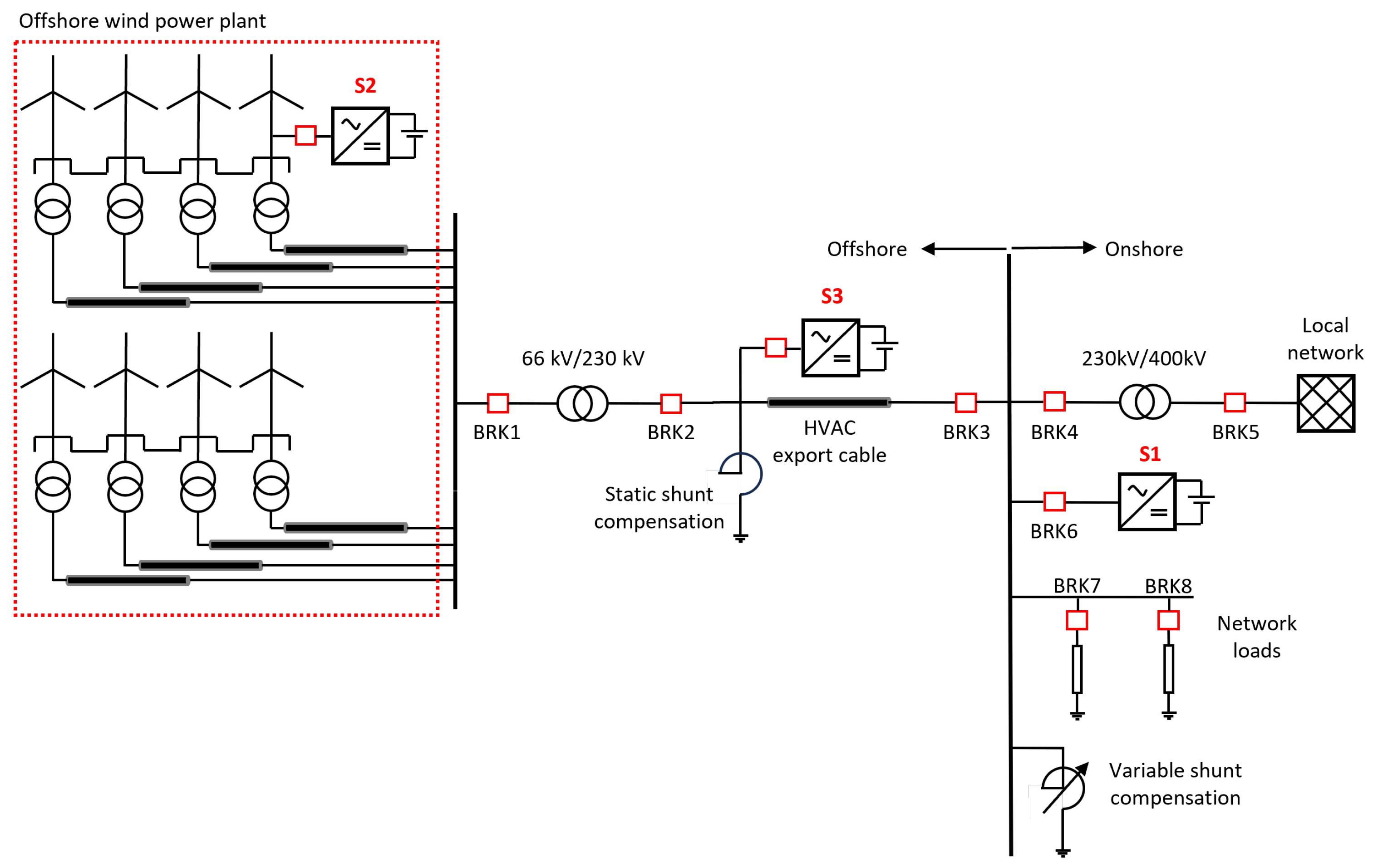
Figure 2.
GFL and GFM control structures schemes.
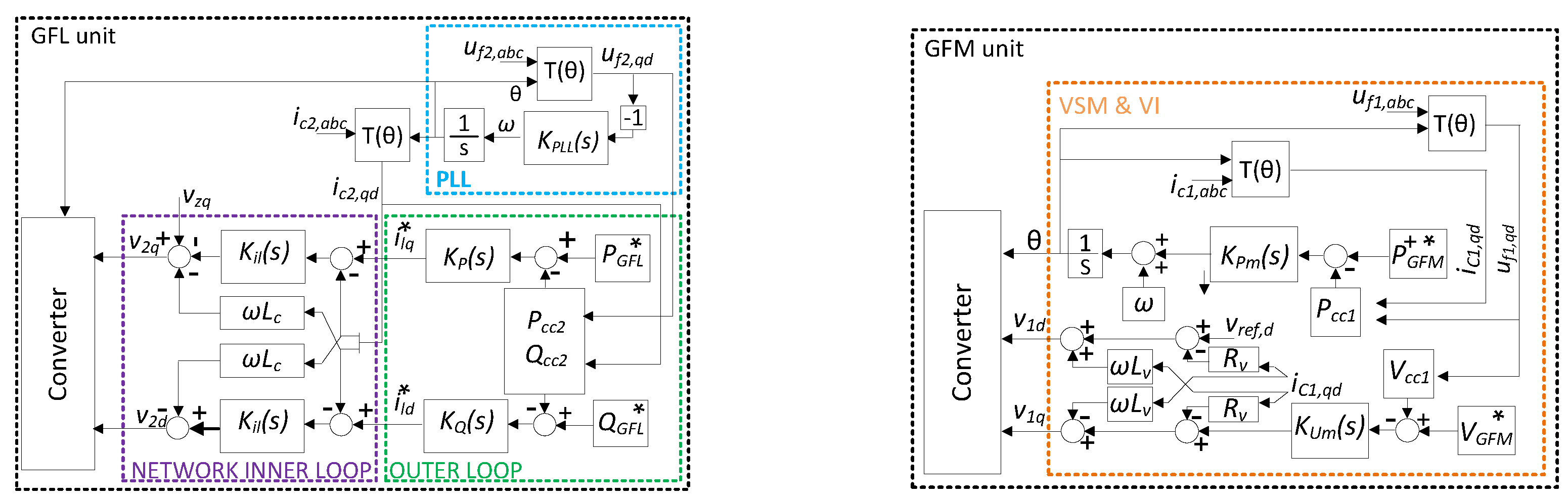
Figure 3.
Diagram of the supervisory frequency support controller.
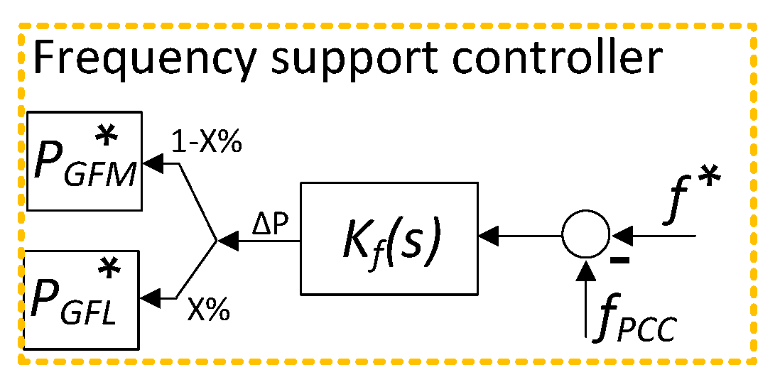
Figure 4.
OWPP and network simplified one-line model.
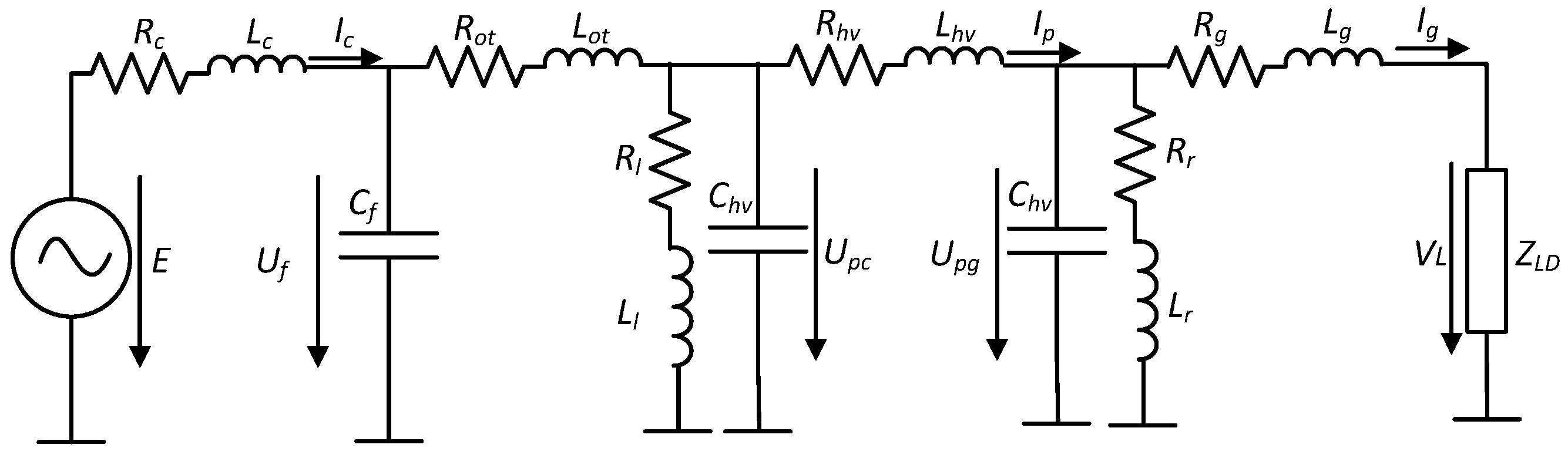
Figure 5.
OWPP and network one-line impedance base model.
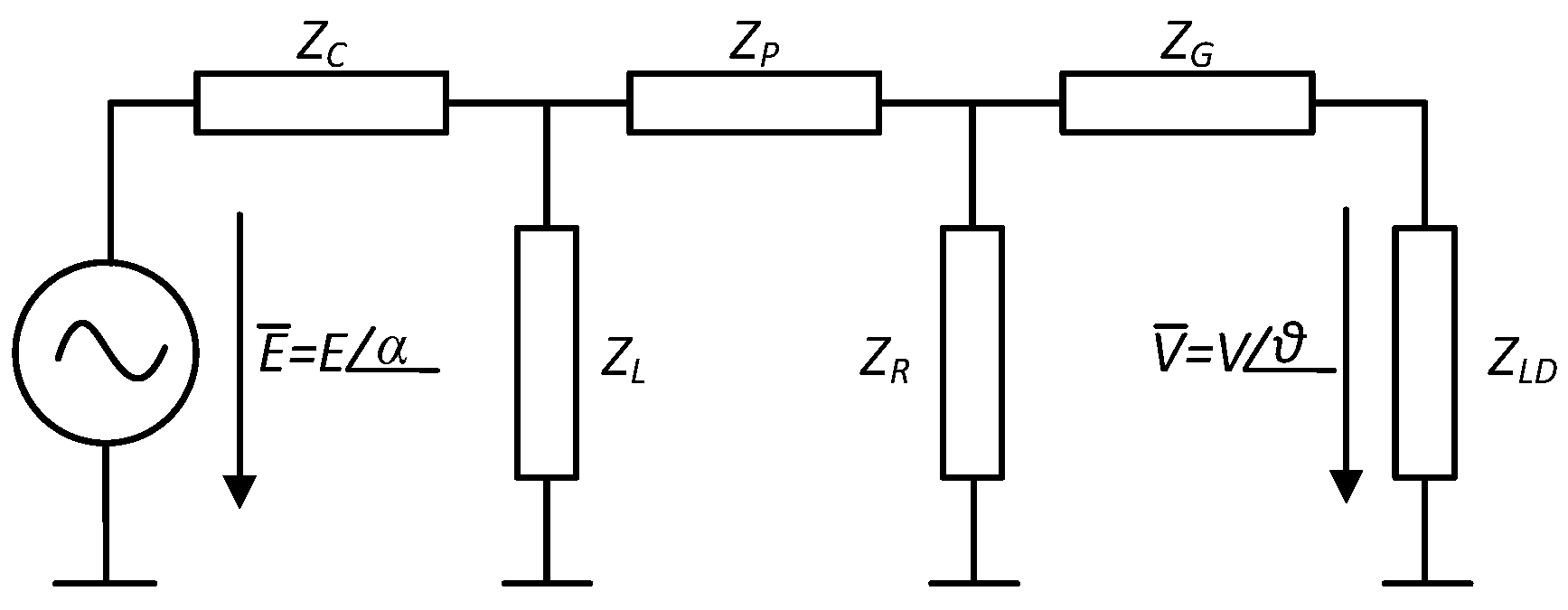
Figure 6.
Energization steps for three different local network demand cases, 1, 2 and 3.
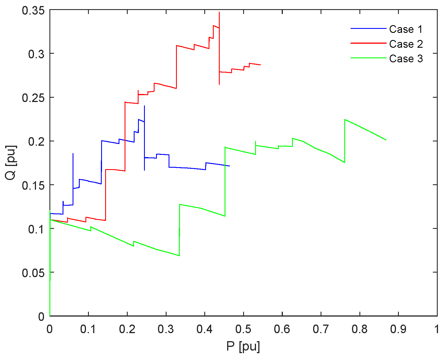
Figure 7.
OWPP and local network (P,Q) OP for cases 1, 2 and 3.
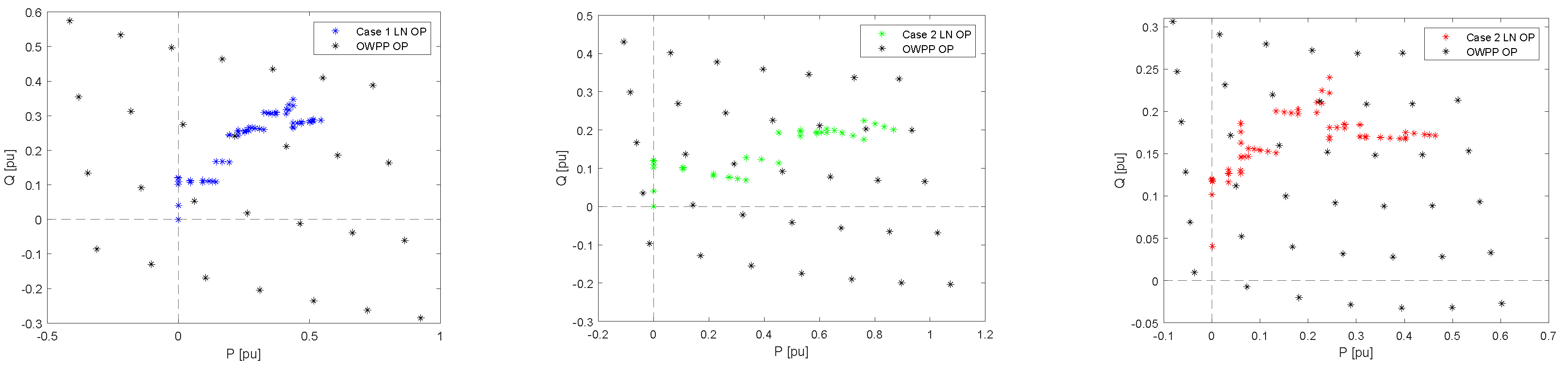
Figure 8.
One-line diagram of the EMT model analysed (NEED TO INCLUDE GRID IN PIC).
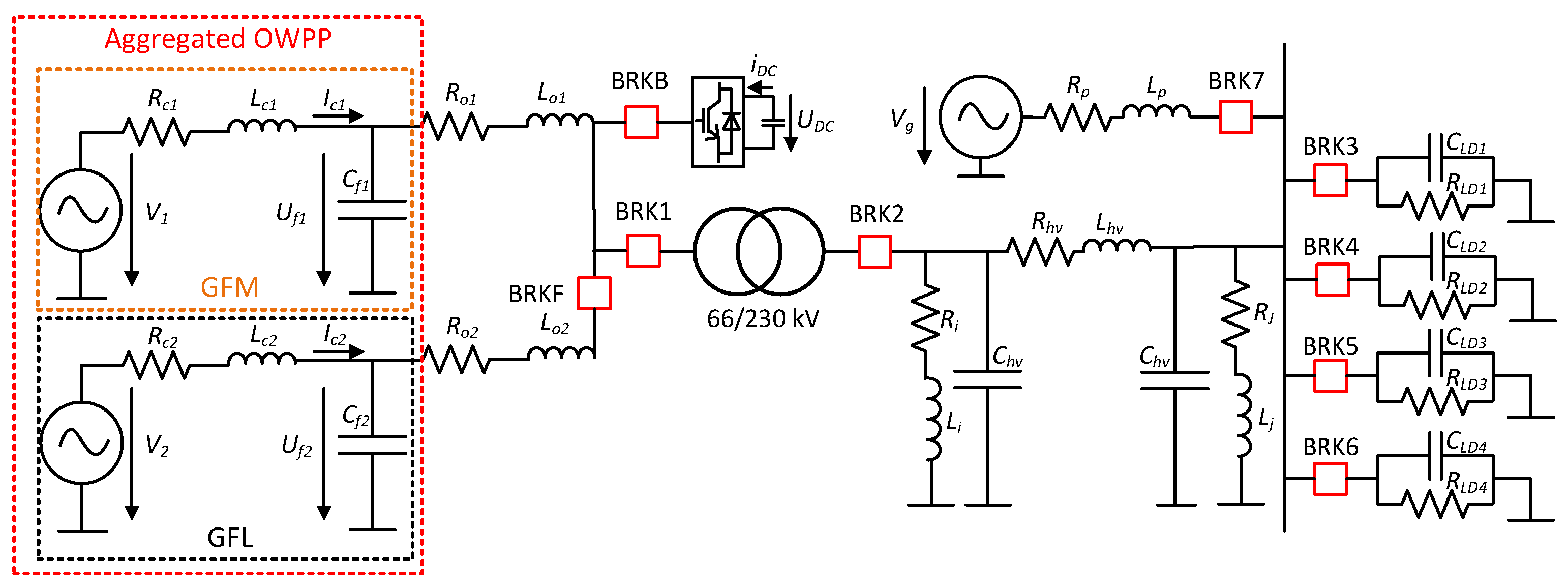
Figure 9.
Offshore transformer energization without any inrush current mitigation technique.
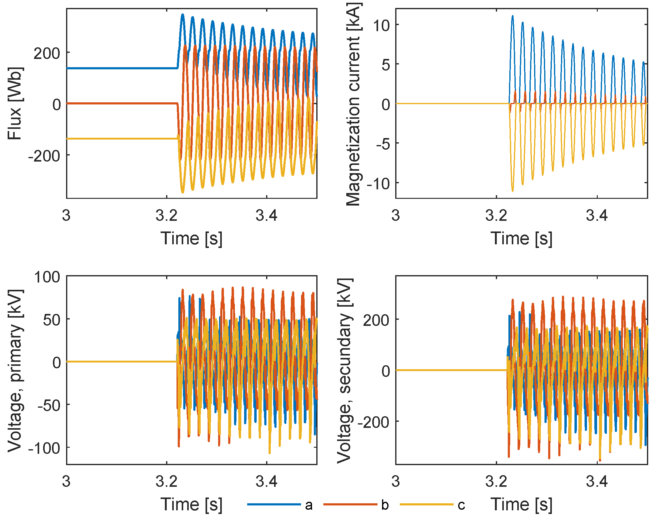
Figure 10.
Offshore transformer energization with POW for a GFM penetration of 20%.
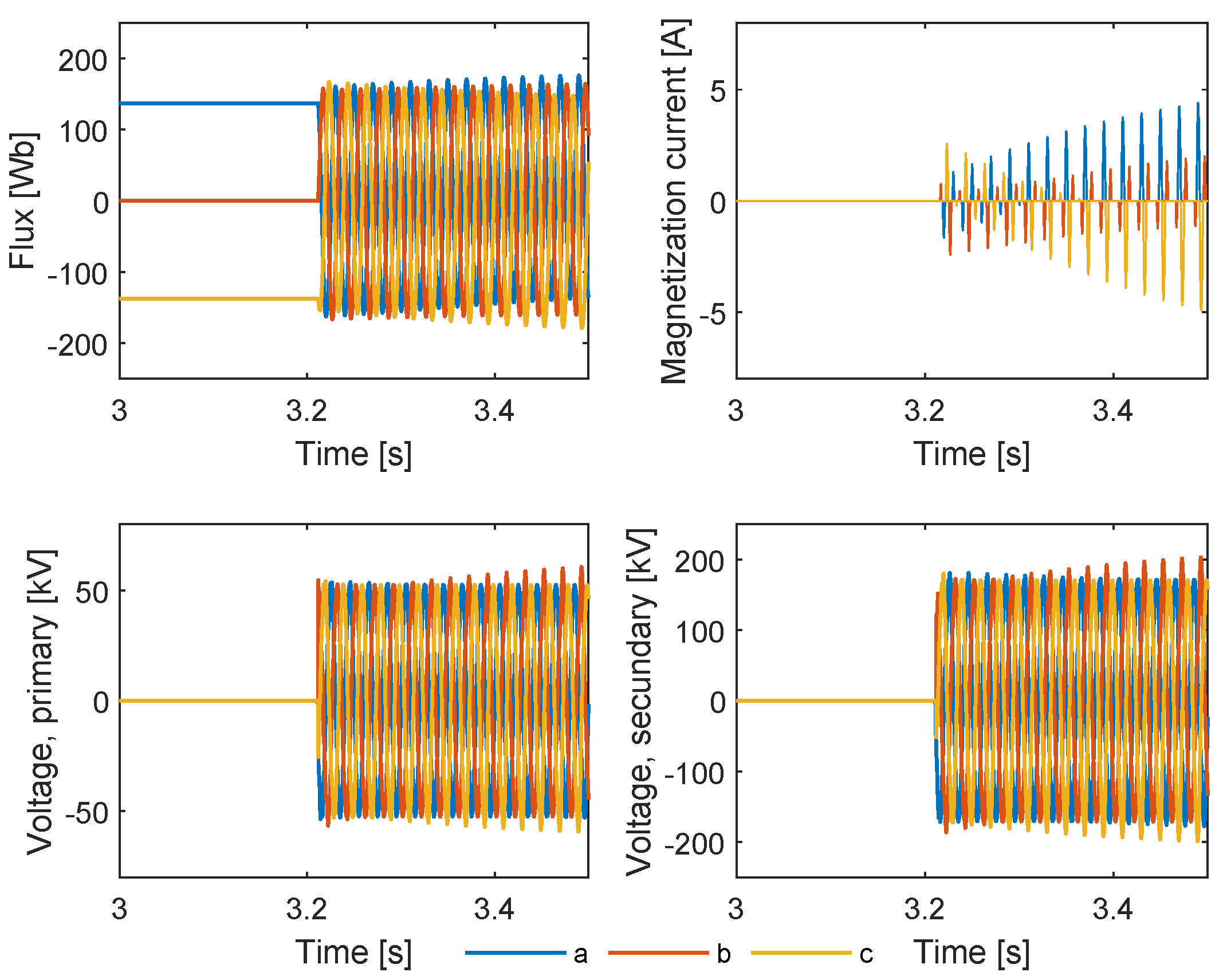
Figure 11.
Inrush currents after transformer energization for different GFM penetration percentages.
Figure 11.
Inrush currents after transformer energization for different GFM penetration percentages.
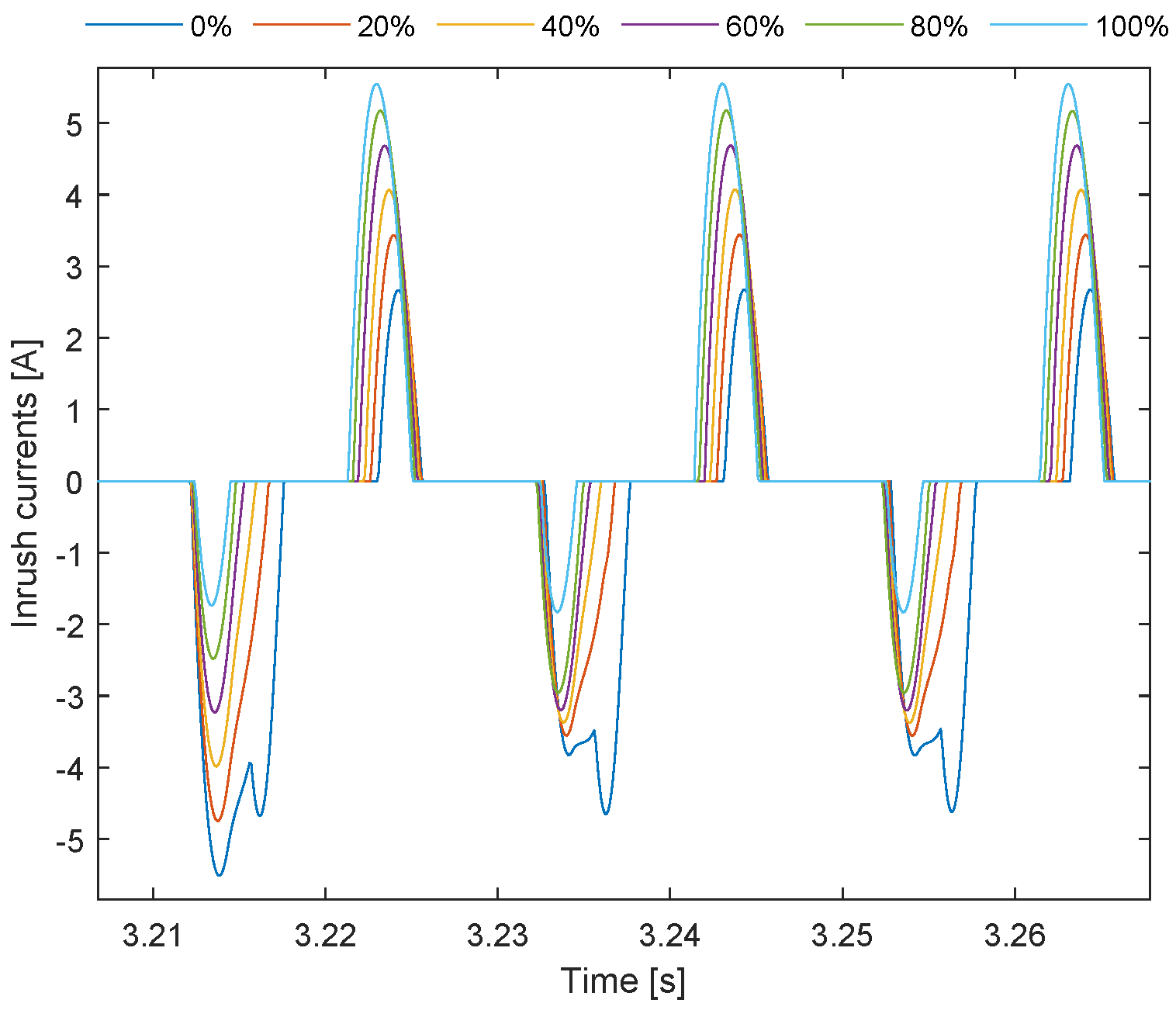
Figure 12.
Cable and shunt reactors compensation for a GFM penetration of 40%.
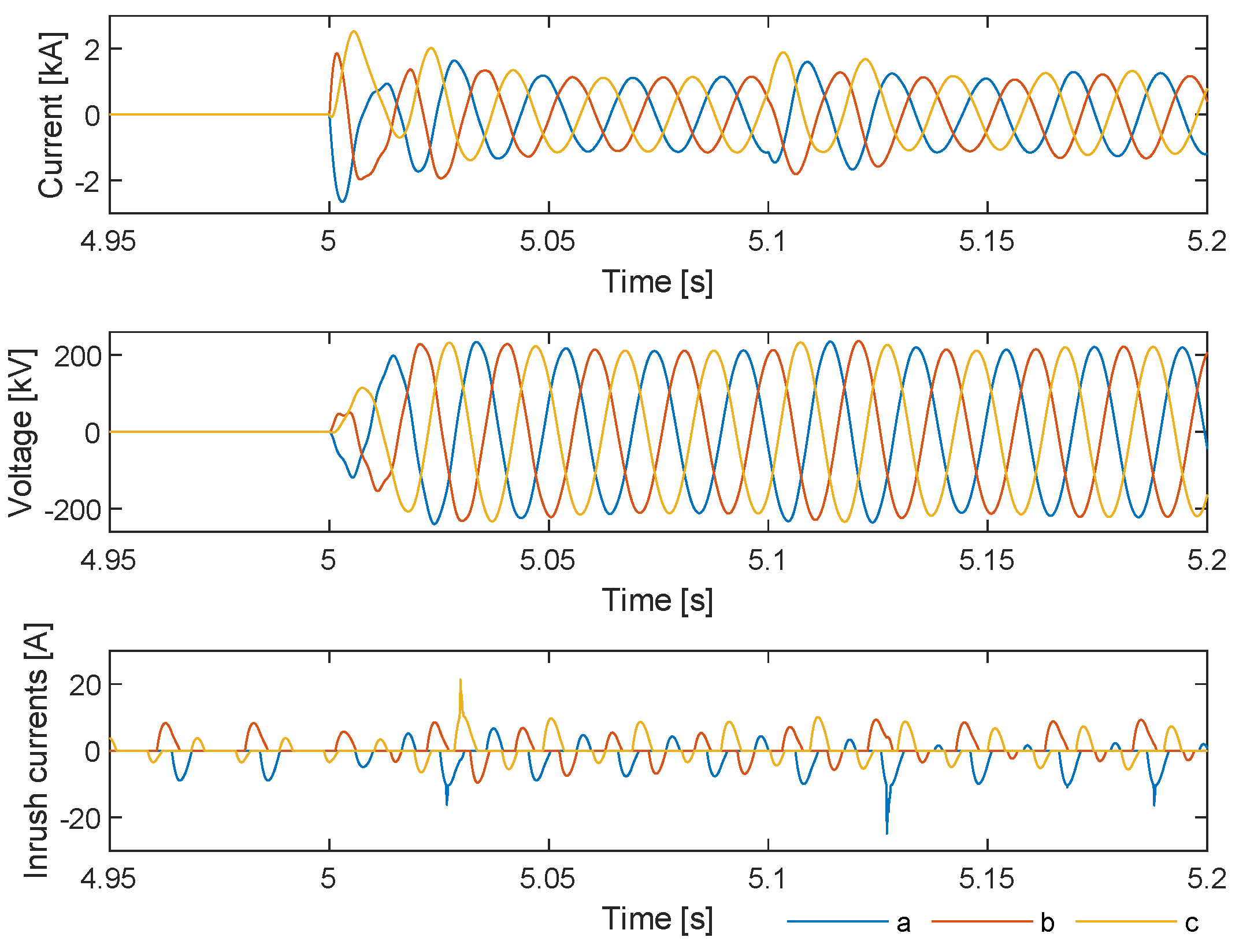
Figure 13.
Inrush currents after cable and shunt compensation energization for different GFM penetration percentages.
Figure 13.
Inrush currents after cable and shunt compensation energization for different GFM penetration percentages.
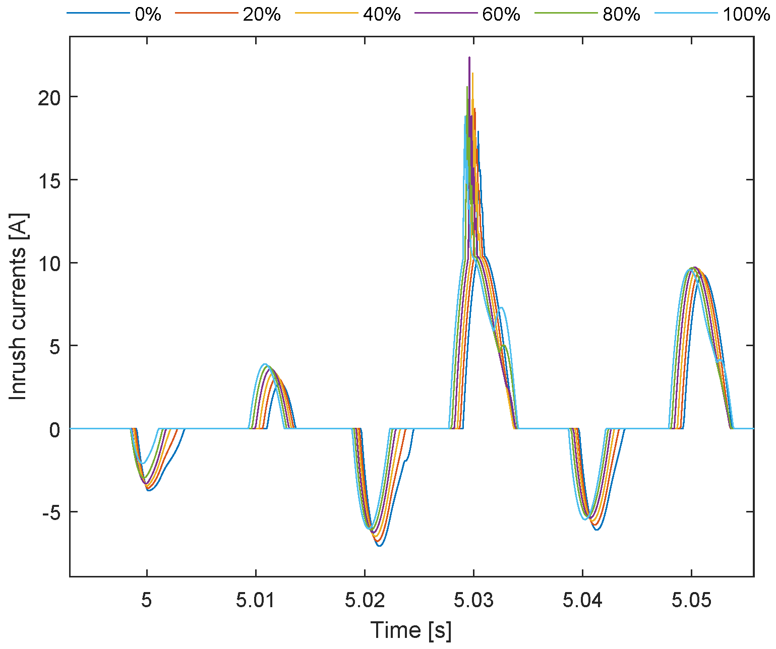
Figure 14.
Active power at the load and converter control action (GFM and GFL) for an 80% GFM penetration during block loading for the top-up scenario.
Figure 14.
Active power at the load and converter control action (GFM and GFL) for an 80% GFM penetration during block loading for the top-up scenario.
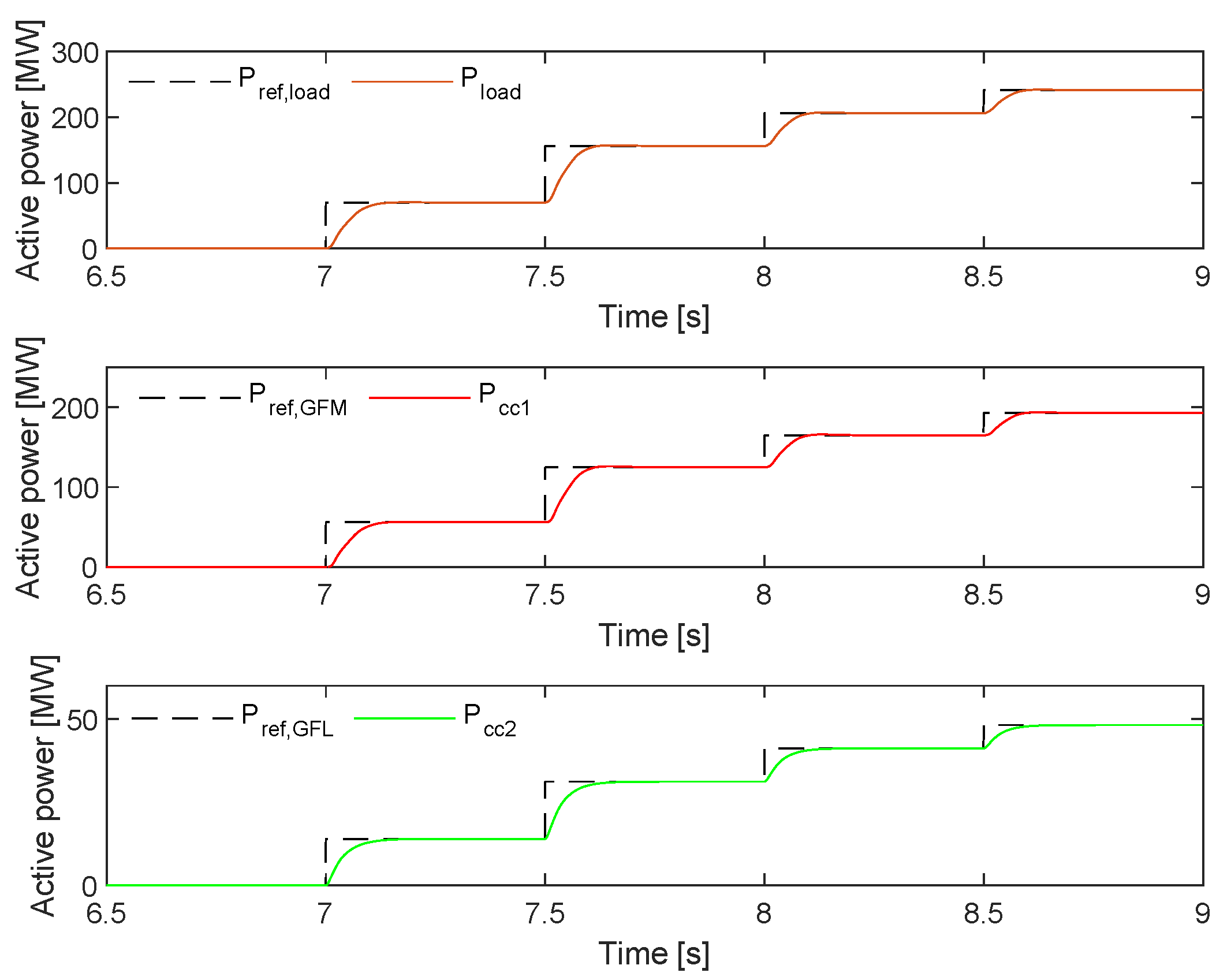
Figure 15.
Voltage and frequency at the PCC during block loading for the different GFM penetrations (from 0% to 100%) for the top-up scenario.
Figure 15.
Voltage and frequency at the PCC during block loading for the different GFM penetrations (from 0% to 100%) for the top-up scenario.
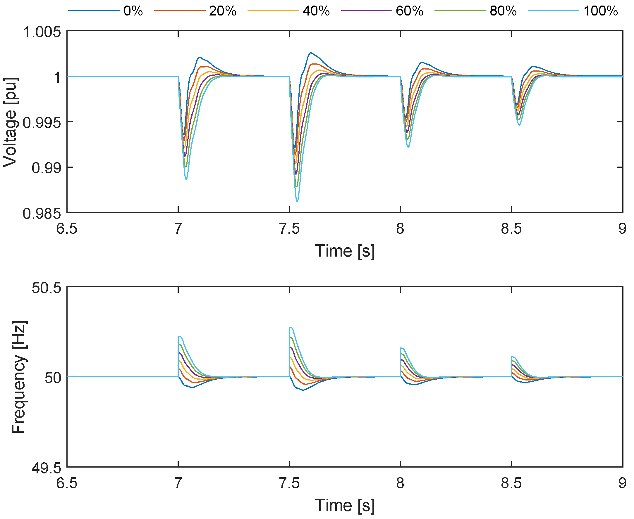
Figure 16.
Voltage and frequency at the PCC during block loading for the different GFM penetrations (from 0% to 100%) without frequency control for the anchor scenario.
Figure 16.
Voltage and frequency at the PCC during block loading for the different GFM penetrations (from 0% to 100%) without frequency control for the anchor scenario.
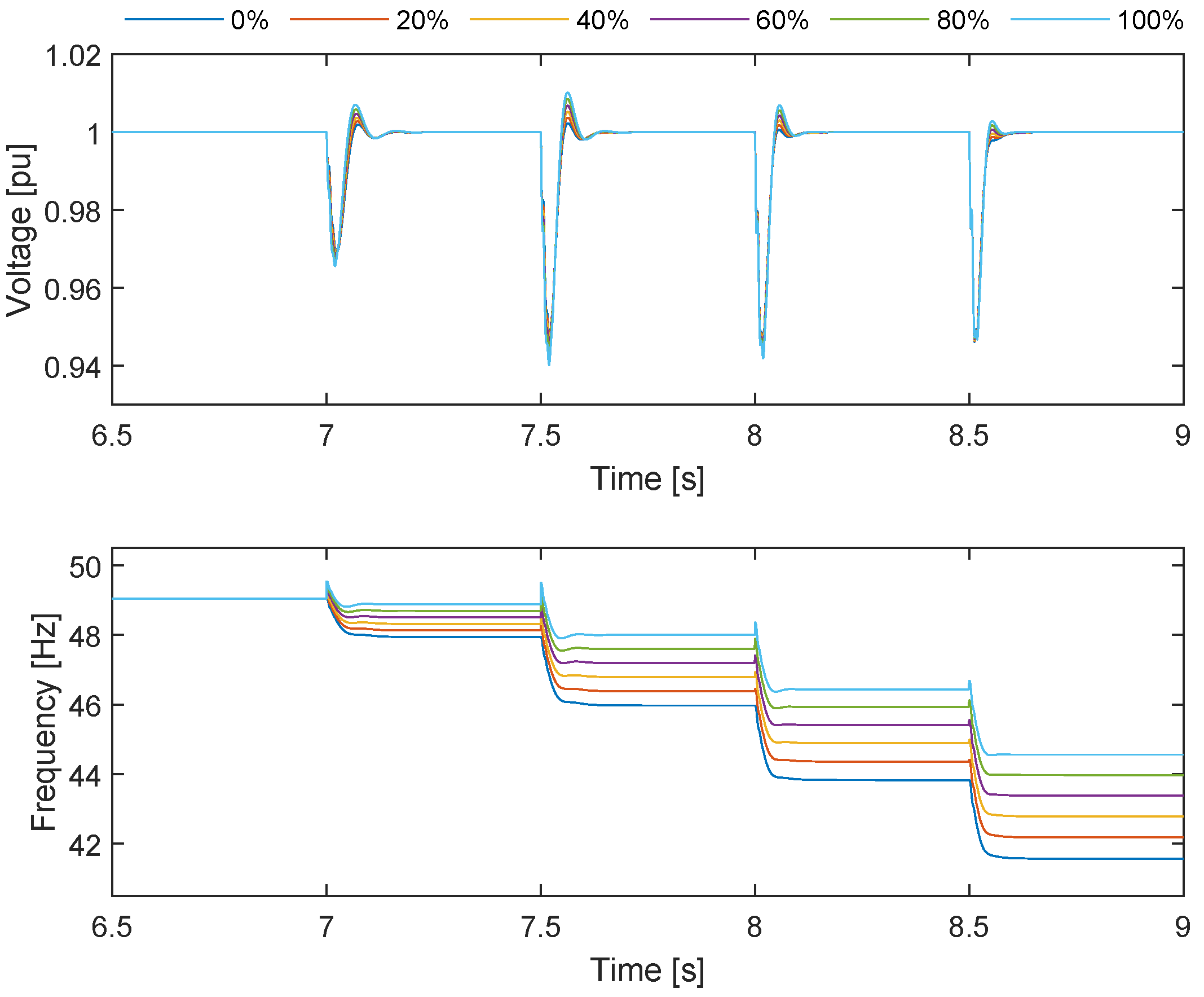
Figure 17.
Voltage and frequency at the PCC during block loading for the different GFM penetrations (from 0% to 100%) with frequency control for the anchor scenario.
Figure 17.
Voltage and frequency at the PCC during block loading for the different GFM penetrations (from 0% to 100%) with frequency control for the anchor scenario.
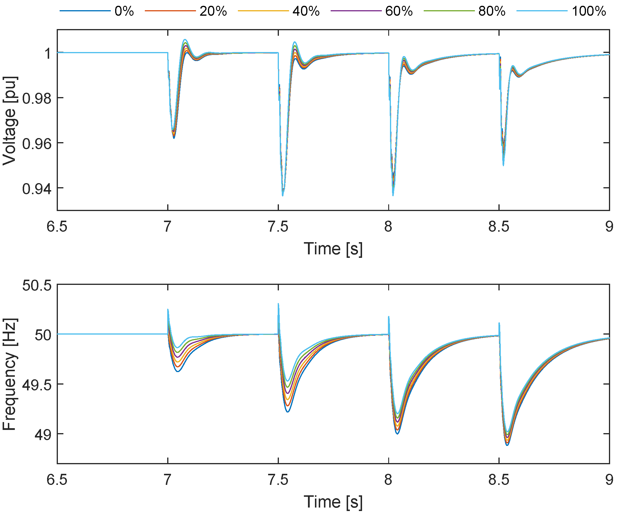
Figure 18.
GFM and GFL converters forming the aggregated wind farms and power system for SSM analysis.
Figure 18.
GFM and GFL converters forming the aggregated wind farms and power system for SSM analysis.

Figure 19.
Scheme of the linearized system (SSM) with both GFM and GFL aggreagted wind farms and controllers and power system.
Figure 19.
Scheme of the linearized system (SSM) with both GFM and GFL aggreagted wind farms and controllers and power system.
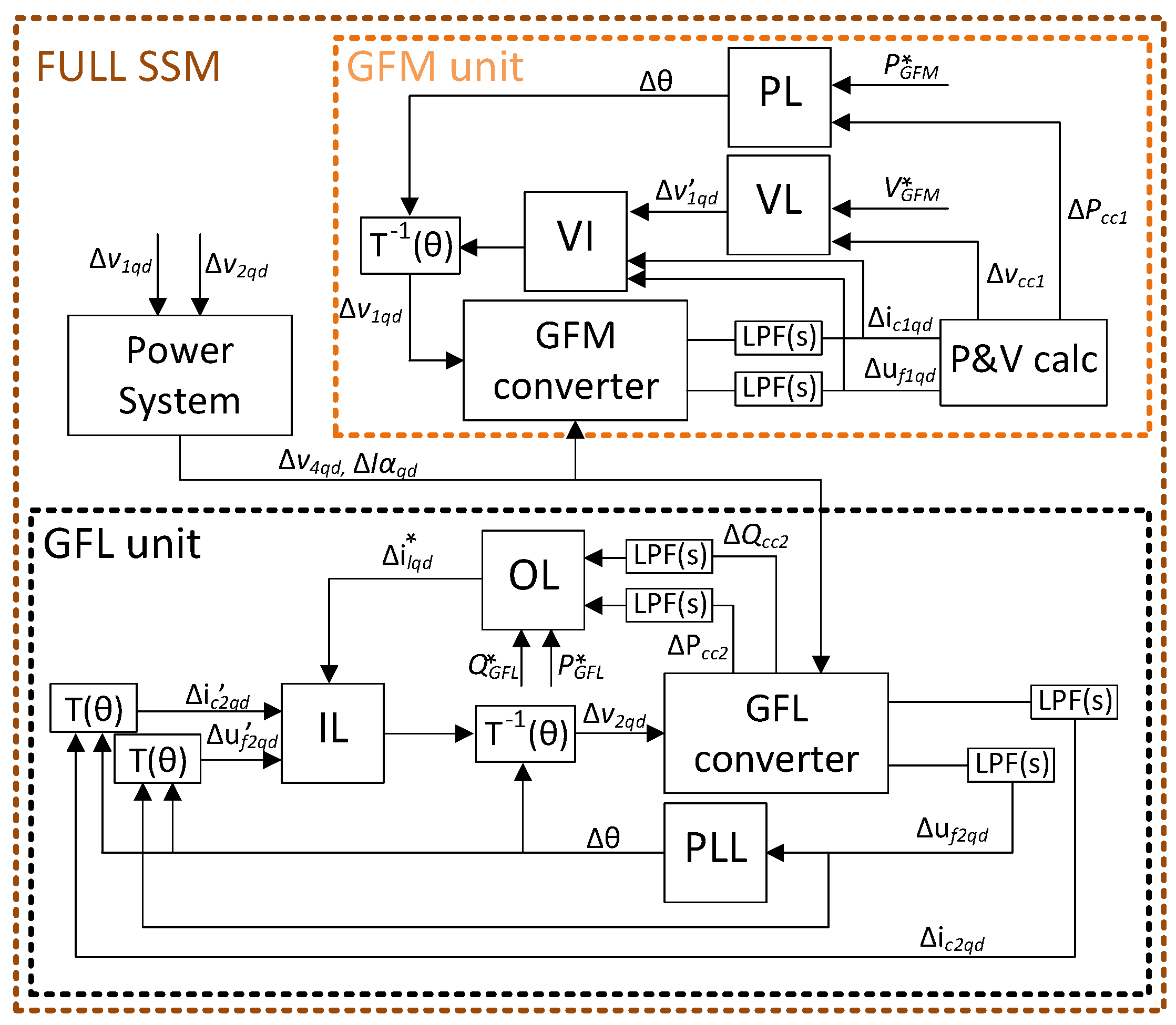
Figure 20.
SSM validation for both GFL (left) and GFM (right) converter controllers: Active power reference, and , PCC active power from EMT model, and , and PCC active power from SSM, and .
Figure 20.
SSM validation for both GFL (left) and GFM (right) converter controllers: Active power reference, and , PCC active power from EMT model, and , and PCC active power from SSM, and .
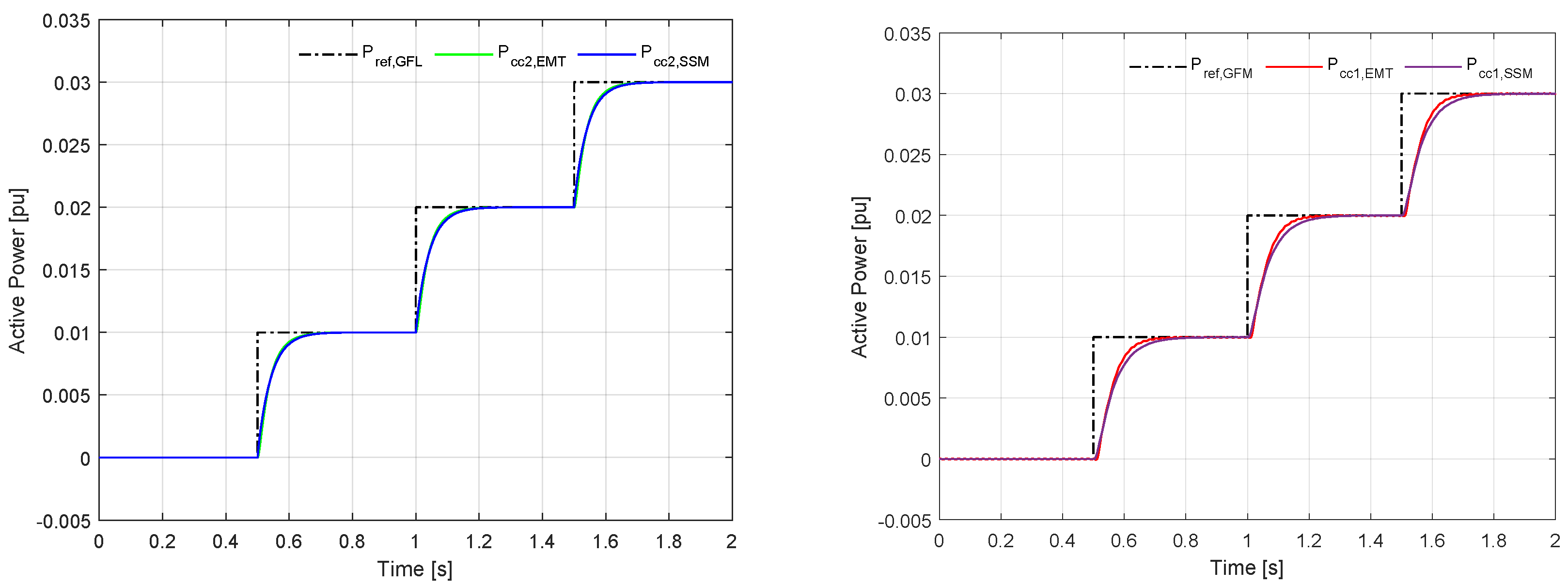
Figure 21.
DM results for the top-up scenario.
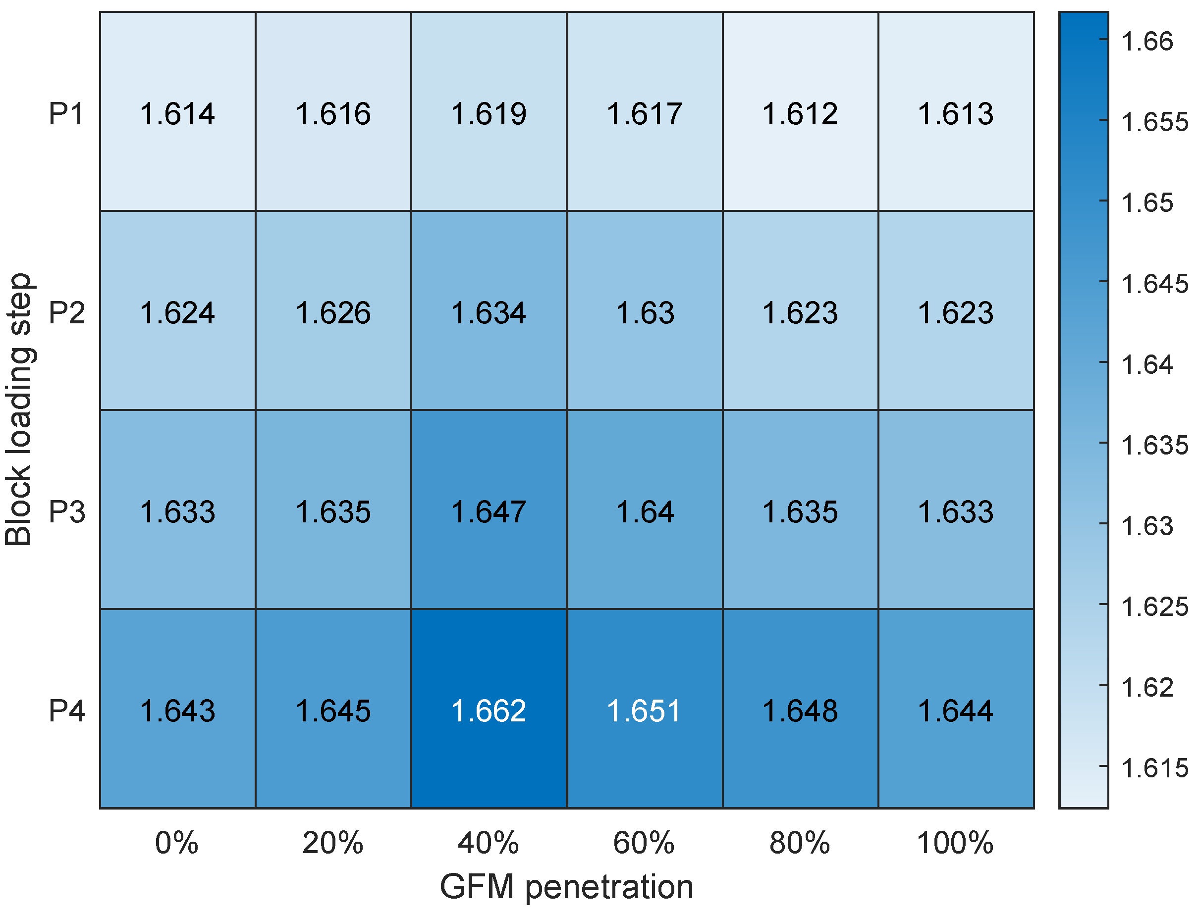
Figure 22.
DM results for the anchor scenario.
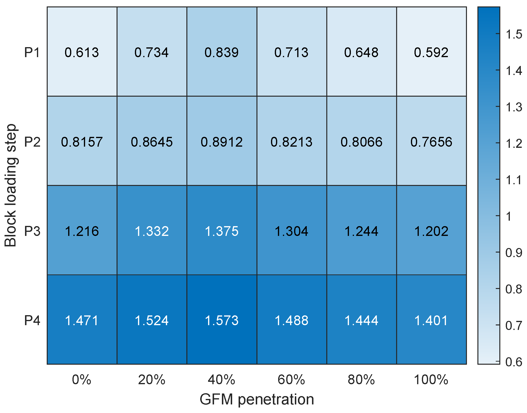
Table 1.
Scenarios for WT-OWPP energization.
| Scenario | APS location | GFM WT required? |
|---|---|---|
| S1 | Onshore | No |
| S2 | Self-start WT | Yes |
| S3 | Offshore | No |
| S4 | Hybrid | No |
Table 3.
Technical requirements analysed via EMT simulations.
| No. | Technical requirement | Range |
|---|---|---|
| 1 | Block loading capability | 35 to 50 MW |
| 2 | Frequency control (while block loading) | 47.5 to 52 Hz |
| 3 | Voltage control (while block loading) | 0.9 to 1.1 pu () |
| 4 | Ability to withstand inrush currents and transient voltages | Analysed during network energization |
| 5 | Reactive range to energise immediate network | 50 MVAr |
Table 4.
Energization sequence of PSR.
| Step | Time (s) | Activity |
|---|---|---|
| 1 | 0 | BRKB is closed and self-start, GFM units, start the energization process |
| 2 | 2 | BRKF is closed to energize the GFL units, hence fully energizing OWPP |
| 3 | 3.2 | BRK1 is closed and offshore transformer is energized |
| 4 | 5 | BRK2 is closed, energizing shunt compensations and submarine export cable |
| 5 | 7 | BRK3 is closed to energize first load (P1) |
| 6 | 9 | BRK4 is closed and second load is energized (P2) |
| 7 | 11 | BRK5 is closed and third load is energized (P3) |
| 8 | 13 | BRK6 is closed and fourth load is energized (P4) |
Table 5.
Top-up generation - Results of EMT simulations for different GFM penetrations.
| No. | 0% | 20% | 40% | 60% | 80% | 100% |
|---|---|---|---|---|---|---|
| 1 | √ | √ | √ | √ | √ | √ |
| 2 | 50 | 50.05 | 50.11 | 50.16 | 50.22 | 50.27 |
| 2 | 49.93 | 49.96 | 49.98 | 49.99 | 50.00 | 50.00 |
| 3 | 1.00 | 1.00 | 1.00 | 1.00 | 1.00 | 1.00 |
| 3 | 0.992 | 0.991 | 0.990 | 0.989 | 0.988 | 0.987 |
| 4 | √ | √ | √ | √ | √ | √ |
| 5 | √ | √ | √ | √ | √ | √ |
Table 6.
Anchor generation - Results of EMT simulations for different GFM penetrations.
| No. | 0% | 20% | 40% | 60% | 80% | 100% |
|---|---|---|---|---|---|---|
| 1 | √ | √ | √ | √ | √ | √ |
| 2 | 50 | 50.06 | 50.12 | 50.18 | 50.25 | 50.31 |
| 2 | 48.88 | 48.91 | 48.94 | 48.96 | 48.99 | 49.02 |
| 3 | 1.00 | 1.00 | 1.00 | 1.00 | 1.00 | 1.00 |
| 3 | 0.939 | 0.938 | 0.938 | 0.937 | 0.937 | 0.936 |
| 4 | √ | √ | √ | √ | √ | √ |
| 5 | √ | √ | √ | √ | √ | √ |
Disclaimer/Publisher’s Note: The statements, opinions and data contained in all publications are solely those of the individual author(s) and contributor(s) and not of MDPI and/or the editor(s). MDPI and/or the editor(s) disclaim responsibility for any injury to people or property resulting from any ideas, methods, instructions or products referred to in the content. |
© 2024 by the authors. Licensee MDPI, Basel, Switzerland. This article is an open access article distributed under the terms and conditions of the Creative Commons Attribution (CC BY) license (http://creativecommons.org/licenses/by/4.0/).
Copyright: This open access article is published under a Creative Commons CC BY 4.0 license, which permit the free download, distribution, and reuse, provided that the author and preprint are cited in any reuse.


