Submitted:
30 November 2024
Posted:
02 December 2024
You are already at the latest version
Abstract
Recent trends in mobility and transportation underscore the growing importance of promoting alternative, flexible, and environmentally friendly modes of transport – such as cycling – that not only contribute significantly to users’ health and well-being but also enable urban concepts like the 15-minute city. For cyclists, travel time is a critical factor influencing both route selection and the decision to choose cycling as a preferred mode of transportation. This paper presents an energy-based model of a synthetic population of free cyclists to analyze their speed profile characteristics, summarized in terms of average speed. The model accounts for key factors such as rolling resistance and aerodynamic drag – both of which vary with ambient temperature – along with acceleration, road gradient, and other influences, including free rolling and deceleration or stopping at intersections and traffic lights. The results reveal a distribution of cycling speeds ranging between 15 and 24 km/h, with a notable concentration around the mean rather than following a normal distribution. The proposed model is intended for use in evaluating infrastructure planning, optimizing green wave traffic light systems, and assessing the health benefits of cycling.
Keywords:
sustainable mobility
; ecological transport
; bicycle
; free cyclist
; micro-simulation
; digital twin
; synthetic population
; energy model
; infrastructure planning
1. Introduction
Bicycling is a key component of sustainable mobility and the 15-minute city concept, as increasing the use of bicycles is often considered a central solution to the challenges of low-emission and (sub-)urban transportation systems [1,2]. Solá and Vilhelmson [3] identified one definition of the 15-minute city – proximity derived from the established principles of transportation and land-use integration – based on insights gathered from respondents, emphasizing the role of urban planners. Several studies, including those by Bovy et al. [4], Stinson et al. [5], Caulfield et al. [6] and Bhat et al. [7], have consistently identified travel time as one of the most critical factors influencing cyclists’ route choices and their decision to use bicycles as a mode of travel. In contrast, traffic planners often need to prioritize cost considerations. For instance, in Sweden, only 2% of the total travel work in 2021 was bone by bike [8], yet just 1% of the national infrastructure budget was allocated to bicycle-related projects. This highlights the need for smart planning tools that not only evaluate costs but also quantify and monetise the benefits of improved cycling infrastructure. To address this need, this paper presents a high-accuracy physical model designed to predict the riding behaviour of free cyclists – those whose movements are not constrained by interactions with other cyclists.
For instance, when constructing a bridge for pedestrians and cyclists over a body of water, the question may arise whether to extend the bridge’s length to also span a nearby road along the shoreline. While the longer bridge would entail higher costs compared to the shorter version, it could significantly reduce the travel time and energy expenditure for cyclists commuting across it – potentially by as much as one minute. This reduction in travel time could make the cycleway accessible to residential areas that are currently beyond the time threshold that commuters are willing to invest. Such an improvement could justify the additional expense by creating value equivalent to the saved time and increased accessibility.
Cycling involves overcoming various driving resistances, such as aerodynamic drag, rolling resistance, climbing resistance, and inertia during acceleration, while simultaneously increasing potential or kinetic energy. The individual cyclist – defined here as a combination of a human being and the bicycle – can influence these driving resistances in several ways. For instance, they can choose clothing that minimizes aerodynamic drag, select tyres or adjust tyre inflation pressure to reduce rolling resistance, plan routes to avoid steep climbs, and adopt a driving style that optimizes energy usage. However, driving resistances are not solely determined by the cyclist. Infrastructure planners and designers also play a significant role. For example, the design of the surrounding environment can influence aerodynamic drag, road surface quality affects rolling resistance, the gradient of cycle paths impacts climbing resistance, and traffic light coordination influences the frequency of decelerations and accelerations. Furthermore, driving resistances, in combination with the cyclist’s available power, are key determinants of travel time – a critical factor influencing route choice and the decision to use cycling as a mode of transport (as noted earlier). This highlights the importance of reducing driving resistances to encourage more people to use bicycles for utility trips (everyday trips where cycling serves as a mode of transport rather than recreation or exercise). A detailed model of the longitudinal dynamics of cyclists can provide insights into where energy expenditure is highest and where efficiency improvements can have the greatest impact.
The proposed model represents a synthetic population of cyclists – a digital twin of the population in terms of power availability on a bicycle – based on a physical model supplemented with statistically validated parameters. This article is structured as follows: First, a review of existing models is presented. Next, the proposed model, consisting of a core model and a shell model, is described in detail, including the parameter data used. This is followed by a discussion of the integration of map data as input and a case study to demonstrate the model’s applicability. Finally, the article concludes with a discussion of the findings, potential applications, and overall conclusions.
2. Review of Research and Existing Models
Eco-driving for motorised vehicles, supported by energy models, has been extensively studied in the past [9]. For heavy vehicles, where fuel consumption represents a significant cost, these models play a vital role for both the vehicle owner and operator. Even the driver’s influence is a known factor that is taken into consideration [10]. Similarly, energy-efficient operation has been a longstanding focus in train transportation, where rolling resistance and track inclination are lower than in road transport, but vehicle and load weights are substantially higher [11].
In the field of bicycling, Barnes [12] developed test equipment for an electric bicycle, which was evaluated against an energy model predicting energy requirements to overcome rolling resistance, aerodynamic drag, and acceleration. This model was also employed to optimize the selection of the electric motor. Prediction and experiment deviated up to 20% from each other.
Many cycling models are based on stochastic approaches. For example, Ma [13] modelled acceleration in cyclists using naturalistic data collected via GNSS (Global Navigation Satellite System) from 11 participants. The main question was the probability for the cyclist to overtake another bike or not. In addition, they combined these data with socio-economic factors and found that both gender and agility of the cyclists affected acceleration. Arnesen et al. [13] used GNSS data from a cycle-to-work project in Trondheim, Norway, to model bicycle speed based on road slope and horizontal curvature, employing a Markov model to account for dependencies between observations. Similarly, Castro et al. [14] identified linear correlations between road gradient and cyclists’ output power.
Liang [15] proposed a hybrid psychological-physical force model for bicycle dynamics, combining physical forces such as driving force, contact force and sliding friction force, with psychological forces as collision avoidance force and attractive force projected in a modelled plane. Hoogendoorn et al. [16] introduced a microscopic bicycle traffic model that considers individual headway, incorporating stochastic variables for both minimum and free headway to represent constrained and unconstrained cyclists.
Johansson et al. [17] highlighted the need for bicycle models, particularly a “free cyclist” model, as a foundational basis for other models. Such a model is crucial because certain cycling resistances, like rolling resistance, aerodynamic drag, and climbing force, are independent of surrounding traffic. Models with a physical foundation, often referred to as energy models, have also been proposed. For example, Iseki and Tingström [18] emphasized the importance of topography, as climbing often constitutes the largest fraction of a cyclist’s energy expenditure. Bigazzi and Tengattini [19] developed a comprehensive energy and speed model for cyclists in 2018, incorporating utility considerations for trips. However, their model treated resistances (e. g. , aerodynamic drag, rolling, and climbing) as constants and omitted speed dynamics.
Human energy conversion and metabolism have been simulated in sports contexts [20] and measured during utility cycling [21]. In team settings, models such as that by Trenchard [22] explored the sorting of cyclists within pelotons into subgroups.
Quasi-static physical models are also available, as compared by Berg [23]. These models calculate energy consumption under constant conditions (e. g. , fixed speed, road inclination, and wind). However, they cannot simulate a cyclist’s energy use along a specific track or account for dynamic changes in conditions.
3. Materials and Methods
This study presents a high-accuracy physical model to predict the driving behaviour of a free cyclist (a cyclist unconstrained by other cyclists). The model simulates the bicycle speed profile and energy consumption over a specified route for a representative population of cyclists. It is structured into two components: a shell, which provides necessary input data (Figure 1), and a core model, which calculates speed and energy usage along the route by means of iterations over small steps (Figure 2).
3.1. Model Shell
The model shell, depicted in Figure , distinguishes itself from other approaches by not relying on the average speed of an “average cyclist”. Instead, it models variability within the cyclist population using a physical model that incorporates track data. While motorized vehicles can typically achieve posted speed limits, this assumption does not hold for cyclists, as even a significant portion of the population cannot sustain speeds of . The model, therefore, allows for detailed characterization of individual cyclists, defined by the parameters outlined in Table 1.
The basic assumption for this model is that each cyclist has a certain amount of power the cyclist can (and is willing to) provide at the pedals when riding. So, each cyclist is characterized by a specific constant power output (). The system weight includes the cyclist’s mass, the bicycle’s mass, and any additional load such as luggage or clothing. Rotating masses (e.g., wheels) are assumed to be accounted for in this total. For aerodynamic drag calculations, the cyclist’s frontal area (A) and drag coefficient () are key parameters, influenced by factors such as body size, clothing, and riding posture. The model also accounts for individual behavioural limits, including maximum speed () and lateral acceleration (), which represent thresholds the cyclist is unwilling to exceed.
The model processes input data and generates the following datasets, structured by road segments (the distance between two geographic points):
- Distance
- Elevation difference ()
- Resulting slope angle ()
- Rolling resistance coefficient ()
- Need for stop
- Maximum bicycle speed based on ()
Specifically, the maximum lateral acceleration from the cyclists characterisation is an important input when evaluating route data. Each road segment is derived from geographic data points, including elevation. The distance between points must exceed 1 cm and preferably be greater than 10 cm. In this study, a minimum spacing of 1 m was used to ensure the calculation of realistic horizontal curve radii. While Arnesen [13] utilises the change of direction from one connection of two data points to the next one, here curves are defined by fitting three consecutive points to a circle, with a minimum allowable radius of 1 m to avoid unrealistically sharp turns.
In addition to lateral acceleration, other factors like junctions, right-of-way rules, and traffic lights further influence bicycle speed. These factors are incorporated into the track data and classified into four speed-reduction levels. The most significant reduction level corresponds to a target speed of zero, while the least reduction requires only free rolling, see Table 2.
3.1.1. Environmental Factors
The default ambient temperature is set to 10°C, reflecting the average for central Europe during the 2011–2020 decade [24], but it can be adjusted based on the model’s application. Air density for aerodynamic drag calculations is temperature-dependent, with drag increasing by approximately 0.4% per degree Kelvin of cooling [25]. Similarly, the rolling resistance coefficient () is temperature-adjusted. Based on prior climate chamber experiments [26] a lookup table was generated to adjust the values Tengattini et al. determined in their field survey [27]. While these field measurements were conducted in summer conditions (above 20°C), the lookup table accounts for colder temperatures. An extract of this lookup table is shown in Table 3. Speed dependency of rolling resistance is excluded due to its negligible impact at typical utility cycling speeds [28].
To prepare the core model, a cyclist’s coasting speed is calculated as a function of road slope, using a constant . For routes with significant variations in rolling resistance, recalculation may be required; however, smaller variations are deemed negligible.
3.1.2. Core Model Execution
The core model iterates through the map data in multiple loops, processing input parameters to generate outputs such as speed profiles, average speed, travel time, and energy consumption. Figure illustrates the shell operation workflow, while Figure 2 details the core model’s computational process.
3.2. Core Model
The core model process is outlined in Figure 2. The model receives input data and processes the route using map data. Each road segment is divided into 1 cm steps to ensure high-resolution calculations, and operations are performed in a steady-state manner at each step.
Speed reductions are determined based on lateral acceleration derived from map data or traffic environment factors (see Table 2). The required preview distance is assumed as given. When a speed reduction is necessary, it takes priority: applied power is reduced or set to zero, and deceleration, bicycle speed, time, and power are adjusted using a predefined deceleration characteristic. A deceleration of is applied for speed adjustments, whereas stopping (target speed < 2 m/s) uses in line with the Guide for the Development of Bicycle Facilities [29].
Otherwise, road slope and maximum bicycle speed are compared to each other to estimate whether free rolling fulfils the cyclists bicycle speed demands. According to the descending slope of the road, power input by the cyclist is reduced. The bicycle can accelerate anyhow, even if power input is set to zero. If necessary, the brakes are applied. Anyhow, during braking no energy is recovered since this is hardly the case at any bicycle today.
For slopes insufficient for free acceleration, the bicycle speed is calculated based on available power and driving resistances (Equations 1 and 2), constrained by the individual cyclist’s maximum speed. Here, the bicycle speed from the previous run is taken and fed in as actual speed. Because of the step size of the error arising from the speed deviation is neglectable.
For the calculation the driver input power is always taken as basis. Power requirements to overcome aerodynamic drag, rolling resistance, and climbing forces are subtracted, leaving residual power available for acceleration until a steady-state speed is achieved or a speed limit is reached. If the cyclist reaches 80% of the maximum speed on a moderate descent, power is reduced to 50%, reflecting satisfaction with a high speed. However, the maximum acceleration is capped at as cyclists typically do not use full power during starts due to gear changes and practical limitations. In addition, there might be gear changes necessary that make the continuous application of full power during acceleration impossible. For steep uphill conditions, the acceleration cap is reduced to to smooth speed transitions. Studies such as [30] have reported a mean acceleration of , supporting these assumptions.
3.3. Cyclist Data
The model is designed as a physical representation of a population of cyclists, using data collected over years from thousands of participants in measurement campaigns. This allows the model to be updated as new data becomes available. Since power is the primary limiting factor for cyclists, determined by physical capacity and willingness to exert effort, particular attention is given to human power generation.
Cyclists’ endurance performance, regardless of training level, can be expressed using maximum oxygen uptake, often normalized by body weight. The American College of Sports Medicine (ACSM) has published data on this metric for men cycling on treadmills, categorized by age groups [31]. Similar data are available for women [32]. By combining these distributions with population weight data, the model estimates maximum available endurance power. For simplicity, the population aged 20–59 years is assumed uniformly distributed, which is supported by findings from Tengattini and Bigazzi [27].
However, commuters and utility cyclists rarely operate at maximum power. Olsson et al. [33] found that, on average, cyclists utilize 65% of their maximum power. Based on this, a power distribution for a specific population can be constructed as visualised in Table 4.
Cyclists also influence aerodynamic resistance through posture, clothing, and other factors. Frontal area and drag coefficient distributions () observed by Tengattini and Bigazzi [27] are incorporated into the model. As their measurements were not normally distributed, their data was taken over and distributed in deciles over the population. These parameters are integrated with velocity and air density, which is calculated as a function of ambient temperature.
Rolling resistance data, also derived from Tengattini and Bigazzi [27], reflects measurements taken during summer months, assuming ambient temperatures of 20°C or higher. At such temperatures, rolling resistance varies minimally. To account for temperature dependence at lower values, characteristics from earlier climate chamber experiments [26] were generalized into a lookup table with a floor of -25°C (i.e., values for -25°C are used for colder conditions).
3.4. Map Data
To simulate the driving behaviour of a free cyclist along a specific path within a (virtual) infrastructure, the model requires accurate map data. These can be sourced from CAD data, electronic maps, or recorded GNSS tracks. Elevation data accuracy is particularly critical, as elevation changes significantly affect energy demand, often constituting a large fraction of total energy consumption.
When sourced from CAD data, elevation accuracy is typically excellent. However, the accuracy of height data derived from GNSS tracks varies. For instance, Ma [34] used a Kalman filter combined with locally weighted regression to improve the reliability of GNSS height data, while Arnesen [13] reported satisfactory results for relative height using GNSS data collected via mobile phones with a simple filtering method.
In this study, map data were obtained using the Graphhopper track creator [35] and combined with elevation data from the Swedish National Mapping, Cadastral, and Land Registration Authority’s map service [36]. Consequently, all evaluations in this study rely on data from Lantmäteriet or CAD data obtained indirectly through printed planning documents.
3.5. Parameter Setting of the Model
All rider input data are provided in deciles across the population, enabling a detailed representation of variability. Combining each of these data points gives a multi-dimensional distribution that will be fed as parameter setting into the model, which processes each configuration through the map data. The model’s output includes distributions for key results, such as average velocity and total energy expenditure. By analyzing these distributions, insights into how different cyclist profiles impact performance under varying conditions can be obtained.
3.6. Case Study
To demonstrate the practical application of the model, a road segment was selected from the planning of a major roadway project in the Stockholm region (V259 Tvärförbindelse Södertörn) in Sweden. Relevant data were extracted from publicly available project documents and adapted for use within the model. Although CAD data would have been preferable for increased precision, such data were unavailable for this study.
Three tracks were analyzed for comparison:
- Existing cycleway: Represents the current infrastructure in use.
- Planned cycleway: Reflects the updated design proposed in the project.
- Highway: Designed primarily for motor vehicles.
The three tracks are visualised in Figure 3 and Figure 4. The technical planning matters served as the basis for simulation, with calculations performed sequentially along the route, moving from the left to the right edges of the maps. Starting and end point were the respective map edges. For the existing cycleway (see green track in Figure 3), the route terminates in a left-hand curve, slightly increasing the total track length. No adjustments were made to account for this variation. A deceleration moment was introduced to simulate the cyclist slowing down while crossing a side road.
In contrast, for the planned cycleway, additional deceleration moments were incorporated to account for three left-hand turns required at cycleway intersections.
Given the short length of the track (less than 1 km), the simulation did not assume the trip began from a standstill. Instead, an initial bicycle speed of was applied to reflect a realistic starting condition.
4. Results
This section presents the outcomes generated by the model using the selected input data. Additionally, the results from applying the model to a case study – focused on a planned intersection of a through highway – are discussed.
4.1. Model Simulation
The model simulated the speed profile and energy demand of a population of cyclists along an arbitrary track representative of commuter routes in the Stockholm region. Geographic and elevation data were manually extracted from the Swedish Mapping, Cadastral, and Land Registration Authority (Lantmäteriet) [36] and converted into GPX format for use in the simulation.
The results, illustrated as a blue graph in Figure 5, show the distribution of average cycling speeds across the population. The median average speed was determined to be ().
4.2. Case Study Results
The results of the case study are presented in Figure 6, which compares the speed distributions for the cyclist population across three different tracks: the existing cycleway, the planned cycleway, and the highway.
While the existing cycleway includes a hill to climb from 300 to distance, the planned cycleway contains a few turns that require the cyclist to slow down. In addition, the planned cycleway includes two smaller inclines at and . The highway profile is the smoothest, featuring an average downward slope of 0.5%, resulting in relatively consistent speeds across most of the cyclist population.
As seen in Figure 3 and Figure 4, the distance to cycle on the planned cycleway is larger than the distance on the existing cycleway (850 m vs. 724 m). Anyhow, the shortest distance is that along the highway (683 m).
Despite the planned cycleway being longer than the existing one, its design allows for higher average speeds. This leads to a disproportionate decrease in travel time, as illustrated in Figure 7. Even though cyclists cover more ground on the planned route, they complete the journey in less time due to fewer challenging inclines and smoother turns. Even the energy expenditure required for cycling decreases on the planned cycleway compared to the existing one. This is primarily due to reduced climbing work, which offset the effects of the increased distance. Cyclists benefit from a more efficient energy profile on the planned cycleway design.
5. Discussion
The proposed model successfully simulates a population of cyclists based on measured distributions of power, mass, aerodynamic drag coefficient, frontal area, and rolling resistance. It also accounts for environmental factors such as temperature, which influence both aerodynamic drag and rolling resistance. This enables the model to replicate real-world cycling conditions and behaviours with reasonable accuracy.
Figure 5 shows the results when simulating the population along a typical commuting distance in the outskirts of Stockholm with high flow and hardly stops. This also explains the quite high median of average velocity that is for female and for male cyclists, in comparison to the findings of Olsson [33] who measured for 10 female and for 10 male commuting cyclists including city centre cycling. However, it fits quite well to the range determined by Fluegel et al. [38] who found average speeds between and for the city of Oslo. The standard deviation of the shown distribution () is smaller than other values in the literature () [39], which can also be seen in the different shapes of the distributions – possibly due to the more uniform test conditions.
For the case study, Figure 6 shows the results of the population of cyclists on different tracks in an existing and planned infrastructure setting, visualised in Figure 3 and Figure 4. The results confirm the common knowledge that road slope is a dominant factor influencing travel time and energy expenditure, aligning with prior research [4,5,6,7]. The increase in travel time seems to be affected by means of inclination [40] and stops (including slow downs) [41] – both factors that rather make cyclists to take a longer way instead [42]. The increase in bicycle speed along advantageous infrastructure is impressive shown by the simulation along the parallel highway that in reality is reserved for motorised traffic (see yellow graph in Figure 6). This results in a far higher average speed for all cyclists. The road inclination, in contrast, slows down the cyclists.
Since the climbing and acceleration work are that dominating and the available power differs quite a lot over the population, the scatter increases when a route includes many uphill segments and/or moments of acceleration. This can be seen by the inclination of the average cycling speed graphs in Figure 6 or in their respective standard deviation (existing cycleway: , planned cycleway: , Highway: )
Depending on the inclination angle, the cyclist will reduce speed only moderate or significant. It is a typical situation where the available power is the limiting factor. Usually, an uphill is approached from a planar road where the bicycle speed is higher. And the cyclists takes this kinetic energy into the slope, decreasing the own velocity, until a new steady-state balance of input power and necessary driving power is found.
This origins from the low power to mass ratio of cyclists. Taking the extreme values of the weakest 5% of the population vs. the strongest 5% on a bicycle, we talk about a range of and . To compare this number to other vehicles operating on public roads: fully loaded trucks operate in the range of 5 – . As commonly known, these vehicles are uphill also limited by their available power. In contrast, passenger cars typically operate in the range of 50 – , however, specifically when equipped with internal combustion engines, they hardly utilise their maximum available power. So, steeper inclines slow cyclists disproportionately, particularly for those with lower power-to-mass ratios.
Consequentially, an important finding is, that the elevation data is critical for reliable simulations. GNSS-based data were found unsuitable due to significant deviations, even with filtering. Even data from Openstreetmap [43] extracted by means of the online tool GraphHopper [35] showed clear deviations from reality. Instead, GNSS based data are only recommended for geo-positioning. Elevation data can then be requested from authoritative sources like official elevation services (e.g., Lantmäteriet).
Another important aspect is the stop time. Stops for e. g. traffic lights depend, of course, on whether the traffic lights show red or green. This is not yet considered in the model and an implementation must depend on how traffic lights are programmed. Depending on the application and the available data it is recommended to simulate stops at traffic lights or intersections incorporating probabilistic or rule-based algorithms to account for red lights, green waves, or cyclist detection systems would enhance its realismt, specifically regarding time and mean velocity.
Moreover, adding a preview feature to account for line-of-sight obstructions and anticipated trajectory adjustments would better reflect cyclist behaviour.
A short-term power boost, i. e. temporary power increases for uphill cycling, is considered according to the findings of [30] but is not yet implemented. Based on the findings of Olsson [33], a boost factor of 1.5 seems reasonable.
The maximum lateral acceleration as one of the characterisations of the cyclist is in the present version a fixed value. However, this value will depend on road conditions, too (e. g. dry, wet, snowy, icy). Depending on the context the model will be applied in, this should be taken into account in a further step of development.
Wind effects are not yet considered but can significantly impact energy requirements, especially at higher winds speeds. With increasing relative wind speed aerodynamics stands for the highest amount of driving force. Since the power needed to overcome aerodynamic drag increases with relative speed powered by three, headwind can become significant already with quite low bicycle speed. Incorporating wind variability, either as known mean wind velocity values or – even better – as wind velocity according to known distribution over time to take the scatter into account, would improve the model’s robustness.
Travel time is a critical factor in route choice, but other qualitative aspects, such as road surface quality and aesthetics, also matter. For example:
In addition to travel time, which is one of the most important factors for cyclists regarding choice of route and motivation for the bicycle as the mode of travel, other qualitative aspects, such as road surface quality and aesthetics, also matter. For example: Cyclists in Dresden, Germany, are willing to take an up to 20% longer route for a better surface quality [44]. Similarly, in Copenhagen, Denmark, cyclists prefer routes with green surroundings or designated cycle tracks, even if these are 0.8 km respective 1.8 km longer [42].
While these preferences are outside the scope of the current model, they are important, too, and could be incorporated through preprocessing or post-processing techniques to account for these factors.
6. Conclusions
In general, the model simulates the speed profile of cyclists effectively, especially considering that the primary objective is not to fine-tune the model for one individual cyclist or bicycle but to represent the variability within a population of cyclists. As highlighted in the discussion, traffic stops, such as those caused by traffic lights, are significant. This model is intended to serve as a practical tool for planners and designers of cycling infrastructure, incorporating these stops to derive comparable metrics that characterize infrastructure quality.
The results clearly illustrate that smoother rides on flat terrain benefit all cyclists, with weaker cyclists gaining the most. Reducing the energy required for climbing and acceleration leaves aerodynamic drag and rolling resistance as the primary resistive forces. For aerodynamic drag, speed is the critical factor, meaning that cyclists with greater power are only moderately faster than those with less power. Meanwhile, rolling resistance remains nearly constant across the speed range considered, making it equally impactful for all riders. Therefore, reducing travel time for cyclists is best achieved by creating smooth, uninterrupted routes and maintaining as level a terrain as possible. Energy-based models like the one proposed here can support during the planning process, evaluating and comparing different infrastructure solutions.
To implement this model effectively, an interface for CAD or high-precision GIS data is essential. Nezval [45] demonstrated a promising approach in this regard. Further research is also required to better understand cyclist behaviour, such as speed selection, which may depend not only on available power but also on other factors, including environmental conditions or personal preferences. For example, while the dynamics of cyclist behaviour at traffic lights are partially understood, factors like foresight, line-of-sight obstructions, and local knowledge remain poorly explored.
Additionally, personal preferences, such as choosing routes with appealing surroundings or high-quality surfaces, are not directly accounted for in the current model but could be incorporated through pre- or post-processing techniques. In contrast, the model as presented can already be applied to simulate traffic light green waves or serve as a foundation for macroscopic models that consider interactions between different road users.
While there is room for further refinement, the proposed model is recommended for testing in evaluating infrastructure measures, designing green-wave traffic light controls, and enabling their real-time adaptation. Beyond infrastructure, the model could also prove valuable in public health research, where utility cycling is increasingly recognized as a tool for promoting health. For example, it could support simulations of lactic acid build-up in utility cyclists under dynamic conditions.
Funding
This research was funded by the national strategic research area TrENoP: Transport Research Environment with Novel Perspectives.
Data Availability Statement
Input data to this publication are public available from the named references. The code is available on request.
Conflicts of Interest
The authors declare no conflicts of interest.
References
- Stockholm Chamber of Commerce. The bicycle empowers Stockholm (in Swedish: Cykeln stärker Stockholm). Website, 2021. Online at https://stockholmshandelskammare.se/sites/default/files/2021-09/2100906_SHK_CykelnStarkerStockholm_Webb_Uppslag-komprimerad.pdf 17th 21. 20 October.
- Cycleplan Stockholm [Internet]. The city of Stockholm; c2022 [cited 2022 Mar 03]. Available from: https://start.stockholm/globalassets/start/om-stockholms-stad/sa-arbetar-staden/trafik/cykelplan.pdf.
- Solá, A.G.; Vilhelmson, B. Negotiating proximity in sustainable urban planning: A Swedish case. Sustainability 2019, 11, 31. [Google Scholar] [CrossRef]
- Bovy, P.; Bradley, P. , Route Choice Analyzed With Stated Preference Approaches. In Transportation demand analysis and issues in travel behavior; Transportation Research Record, Transportation Research Board, 1985; pp. 11–20.
- Stinson, M.; Bhat, C. An Analysis of Commuter Bicyclist Route Choice Using a Stated Preference Survey. Transportation Research Board. National Research Council, Washington, DC, 2003, number 03-3301.
- Caulfield, B.; Brick, E.; McCarthya, O. Determining bicycle infrastructure preferences – A case study of Dublin. Transportation Research Part D: Transport and Environment 2012, 17, 413–417. [Google Scholar] [CrossRef]
- Bhat, C.R.; Dubey, S.K.; Nagel, K. Introducing non-normality of latent psychological constructs in choice modeling with an application to bicyclist route choice. Transportation Research. Part B: Methodological 2015, 78, 341–363. [Google Scholar] [CrossRef]
- Dahlstrand, A.; Mattsson, F. National Cycling report 2021 (in Swedish: Nationellt Cykelbokslut 2021). Technical report, Swedish Transport Administration (Trafikverket), 2022. https://trafikverket.diva-portal.org/smash/get/diva2:1681695/FULLTEXT01.pdf.
- Turri, V.; Besselink, B.; Johansson, K. Cooperative Look-Ahead Control for Fuel-Efficient and Safe Heavy-Duty Vehicle Platooning. IEEE Transactions on Control Systems Technology 2017, 25, 12–28. [Google Scholar] [CrossRef]
- Savković, T.; Miličić, M.; Tanackov, I.; Pitka, P.; Koleška, D. Short-term and long-term impacts of eco-driving on dynamics of driving behaviour and operating parameters. Transport (Vilnius, Lithuania) 2020, 35, 143–155. [Google Scholar] [CrossRef]
- Lukaszewicz, P. Energy saving driving methods for freight trains. Advances in Transport 2004, 15, 901–909. [Google Scholar]
- Barnes, M.; Brennan, S. Simulation, design, and verification of an electrified bicycle energy model. ASME 2012 5th Annual Dynamic Systems and Control Conference Joint with the JSME 2012 11th Motion and Vibration Conference, 2012-MOVIC 2012 DSCC, 2012, Vol. 1, pp. 875–880.
- Arnesen, P.; Malmin, O.; Dahl, E. A forward Markov model for predicting bicycle speed. Transportation (Dordrecht) 2020, 47, 2415–2437. [Google Scholar] [CrossRef]
- Pérez Castro, G.; Johansson, F.; Olstam, J. A Power-Based Approach to Model the Impact of Gradient in Bicycle Traffic Simulation. Proceedings of Transportation Research Board 102nd Annual Meeting. Washington DC, United States, - 12, 2023, 2023. 8 January.
- Liang, X.; Mao, B.; Xu, Q. Psychological-Physical Force Model for Bicycle Dynamics. J Transpn Sys Eng & IT 2012, 12, 91–97. [Google Scholar]
- Hoogendoorn, S.; Daamen, W. Bicycle headway modelling and its applications. Transportation Research Record 2016, 2587, 34–40. [Google Scholar] [CrossRef]
- Johansson, F.; Liu, C.; Ekström, J.; Olstam, J. Modelling of bicycle traffic - analysis of needs and knowledge (Cykeltrafikmodellering - Behovsanalys och kunskapsläge). Technical Report 1064, Swedish National Road and Transport Research Institute (VTI), 2020. [Google Scholar]
- Iseki, H.; Tingstrom, M. A new approach for bikeshed analysis with consideration of topography, street connectivity, and energy consumption. Computers, environment and urban systems 2014, 48, 166–177. [Google Scholar] [CrossRef]
- Bigazzi, A.; Lindsey, R. A utility-based bicycle speed choice model with time and energy factors. Transportation (Dordrecht) 2018, 46, 995–1009. [Google Scholar] [CrossRef]
- van Beek, J.; Supandi, F.; Gavai, A.; de Graaf, A.; Binsl, T.; Hettling, H. Simulating the physiology of athletes during endurance sports events: modelling human energy conversion and metabolism. Philosophical Transactions of the Royal Society of London. Series A: Mathematical, physical, and engineering sciences 2011, 369, 4295–4315. [Google Scholar] [CrossRef]
- Schantz, P.; Wahlgren, L.; Eriksson, J.; Sommar, J.; Rosdahl, H. Estimating duration-distance relations in cycle commuting in the general population. PLoS ONE 2018, 13. [Google Scholar] [CrossRef]
- Trenchard, H.; Ratamero, E.; Richardson, A.; Perc, M. A deceleration model for bicycle peloton dynamics and group sorting. Applied Mathematics and Computation 2015, 251, 24–34. [Google Scholar] [CrossRef]
- Berg, S. Sustainable Accessible Cycling (in Swedish: Hållbar Tillgänglig Cykling). Technical report, Ramböll Sverige AB, 2017.
- German Meteorological Service (Deutscher Wetterdienst)., 2021. https://opendata.dwd.de/climate_environment/CDC/regional_averages_DE/monthly/air_temperature_mean/.
- Gressmann, M. Fahrradphysik und Biomechanik : Technik, Formeln, Gesetze, 12. ed. ed.; Delius Klasing: Bielefeld, 2017. [Google Scholar]
- Rothhämel, M. On rolling resistance of bicycle tyres with ambient temperature in focus. Int. J. of Vehicle Systems Modelling and Testing 2023, 17, 67–80. [Google Scholar] [CrossRef]
- Tengattini, S.; Bigazzi, A. Physical characteristics and resistance parameters of typical urban cyclists. Journal of Sports Sciences 2018, 36, 2383–2391. [Google Scholar] [CrossRef]
- Baldissera, P.; Delprete, C.; Rossi, M.; Zahar, A. Experimental Comparison of Speed-Dependent Rolling Coefficients in Small Cycling Tires. Tire science & technology 2021, 49, 224–241. [Google Scholar]
- of State Highway, A.A. ; on Geometric Design. Content Provider, T.O.T.F. Guide for the development of bicycle facilities, 2012. [Google Scholar]
- Parkin, J.; Rotheram, J. Design speeds and acceleration characteristics of bicycle traffic for use in planning, design and appraisal. Transport Policy 2010, 17, 335–341. [Google Scholar] [CrossRef]
- of Sports Medicine, A.C.; Whaley, M.; Brubaker, P.; Otto, R.; Armstrong, L. ACSM’s Guidelines for Exercise Testing and Prescription; Lippincott Williams & Wilkins, 2006.
- Porcari, J.; Bryant, C.; Comana, F. Exercise Physiology; Foundations of exercise science series, F. A. Davis Company, 2015.
- Olsson, K.; Ceci, R.; Wahlgren, L.; Rosdahl, H.; Schantz, P. Perceived exertion can be lower when exercising in field versus indoors. PloS one 2024, 19, e0300776–e0300776. [Google Scholar] [CrossRef] [PubMed]
- Ma, X.; Luo, D. Modeling cyclist acceleration process for bicycle traffic simulation using naturalistic data. Transportation Research. Part F, Traffic Psychology and Behaviour 2016, 40, 130–144. [Google Scholar] [CrossRef]
- GraphHopper., 2021. www.graphhopper.com/.
- Swedish Mapping, Cadastral and Land Registration Authority (Lantmäteriet)., 2021. https://minkarta.lantmateriet.se/.
- Swedish Transport Administration., 2021. www.trafikverket.se/nara-dig/Stockholm/vi-bygger-och-forbattrar/Tvarforbindelse-Sodertorn/dokument/.
- Flügel, S.; Hulleberg, N.; Fyhri, A.; Weber, C.; Ævarsson, G. Empirical speed models for cycling in the Oslo road network. Transportation (Dordrecht) 2017, 46, 1395–1419. [Google Scholar] [CrossRef]
- Twisk, D.; Stelling, A.; Van Gent, P.; De Groot, J.; Vlakveld, W. Speed characteristics of speed pedelecs, pedelecs and conventional bicycles in naturalistic urban and rural traffic conditions. Accident analysis and prevention 2021, 150, 105940–105940. [Google Scholar] [CrossRef]
- Menghini, G.; Carrasco, N.; Schüssler, N.; Axhausen, K. Route choice of cyclists in Zurich. Transportation research. Part A, Policy and practice 2010, 44, 754–765. [Google Scholar] [CrossRef]
- Broach, J.; Dill, J.; Gliebe, J. Where do cyclists ride? A route choice model developed with revealed preference GPS data. Transportation Research Part A: Policy and Practice 2012, 46, 1730–1740. [Google Scholar] [CrossRef]
- Vedel, S.; Jacobsen, J.; Skov-Petersen, H. Bicyclists’ preferences for route characteristics and crowding in Copenhagen – A choice experiment study of commuters. Transportation Research Part A: Policy and Practice 2017, 100, 53–64. [Google Scholar] [CrossRef]
- OpenStreetMap., 2021. www.openstreetmap.org.
- Hagemeister, C.; Schmidt, A. Which criteria own which level of importance for the choice of route for utility cyclists? (In German: Wie wichtig sind welche Kriterien für die Routenwahl von Alltagsradfahrern?). Straßenverkehrstechnik 2003, 47, 313–321. [Google Scholar]
- Nezval, P. Geographic Analysis of Distance and Accessibility for Wheeled Vehicles, Licentiate thesis, KTH Stockholm, 2024. PhD thesis, KTH, Royal Institute of Technology, 2024.
Figure 1.
Visualisation of the shell process of the model.
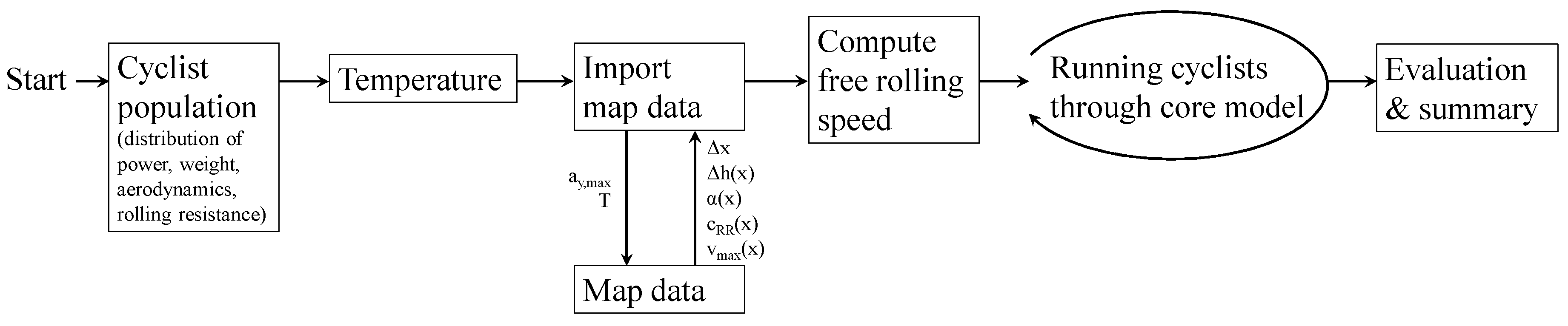
Figure 2.
Visualisation of the core model.
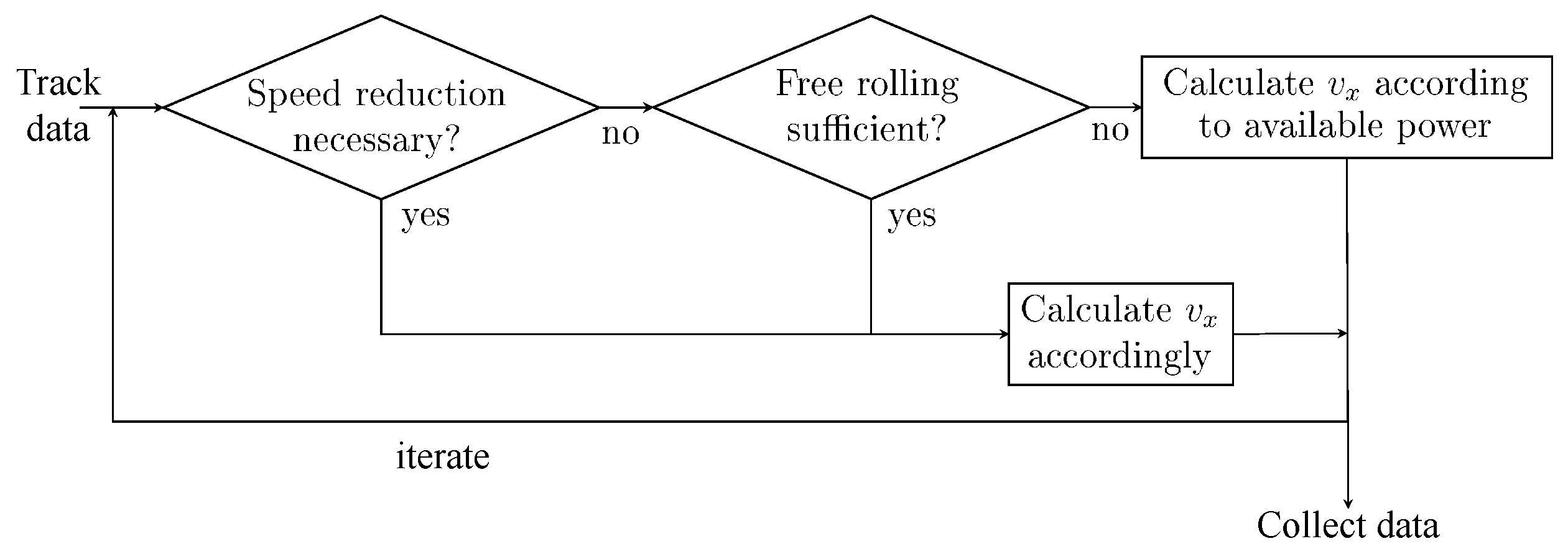
Figure 3.
Visualisation of the CAD data of a planned infrastructure [37]. The added green line marks the existing cycleway.
Figure 3.
Visualisation of the CAD data of a planned infrastructure [37]. The added green line marks the existing cycleway.
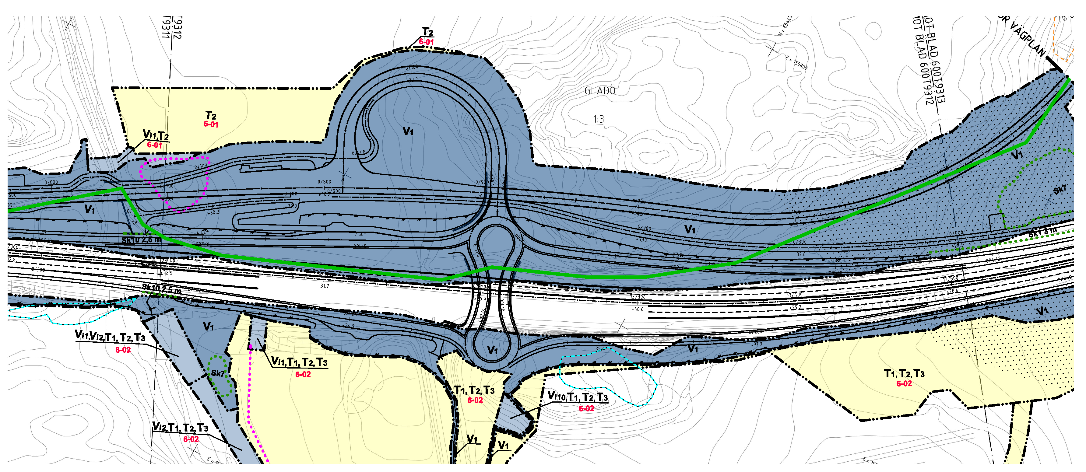
Figure 4.
Illustrationmap of the planned infrastructure [37]. The added magenta line marks the track along the planned cycleway used in this simulation. The added red line marks the track along the planned highway that mainly follows the already existing highway.
Figure 4.
Illustrationmap of the planned infrastructure [37]. The added magenta line marks the track along the planned cycleway used in this simulation. The added red line marks the track along the planned highway that mainly follows the already existing highway.
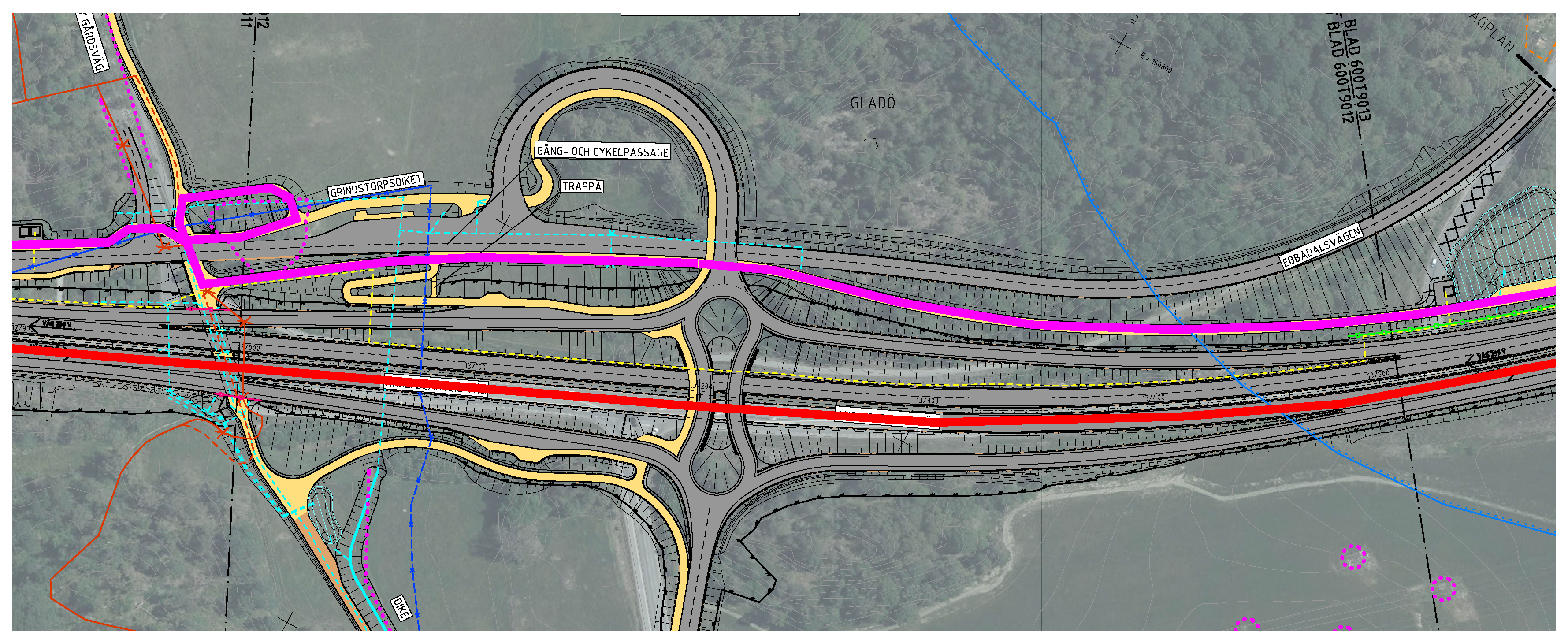
Figure 5.
Distribution of average speed of a population of cyclists (in the age of 20-59 years) simulated over deciles of cyclist’s mass-, power-, rolling resistance- and ()- distribution along a typical cycling commuter track in the outskirts of Stockholm. There are a few very slow and a few very fast cyclists. The main part (80%) is within a range of 15 – .
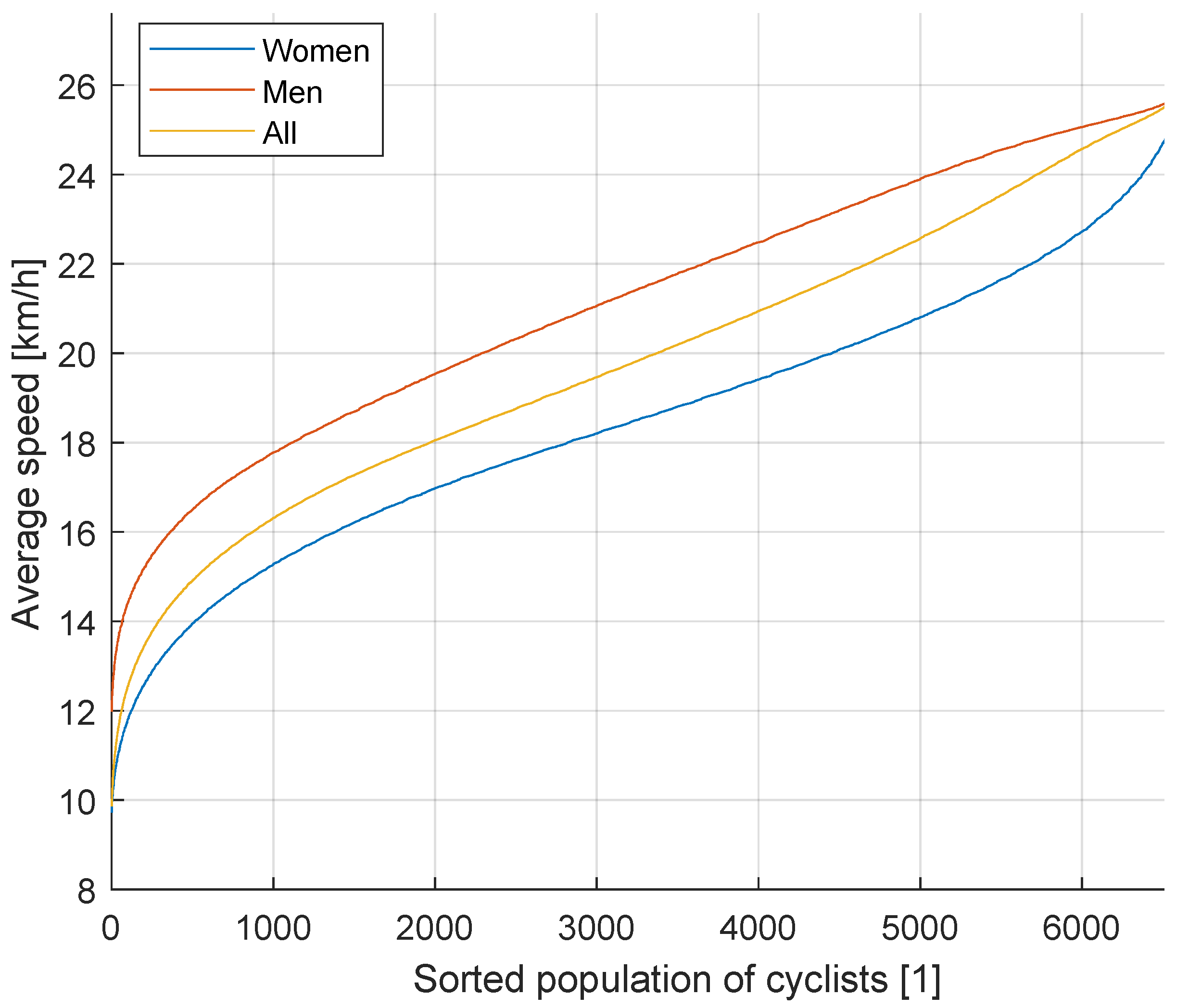
Figure 6.
Bicycle speed distribution of the simulated cyclist population along the three tracks: existing cycleway (blue), planned cycleway (red) and highway (yellow).
Figure 6.
Bicycle speed distribution of the simulated cyclist population along the three tracks: existing cycleway (blue), planned cycleway (red) and highway (yellow).
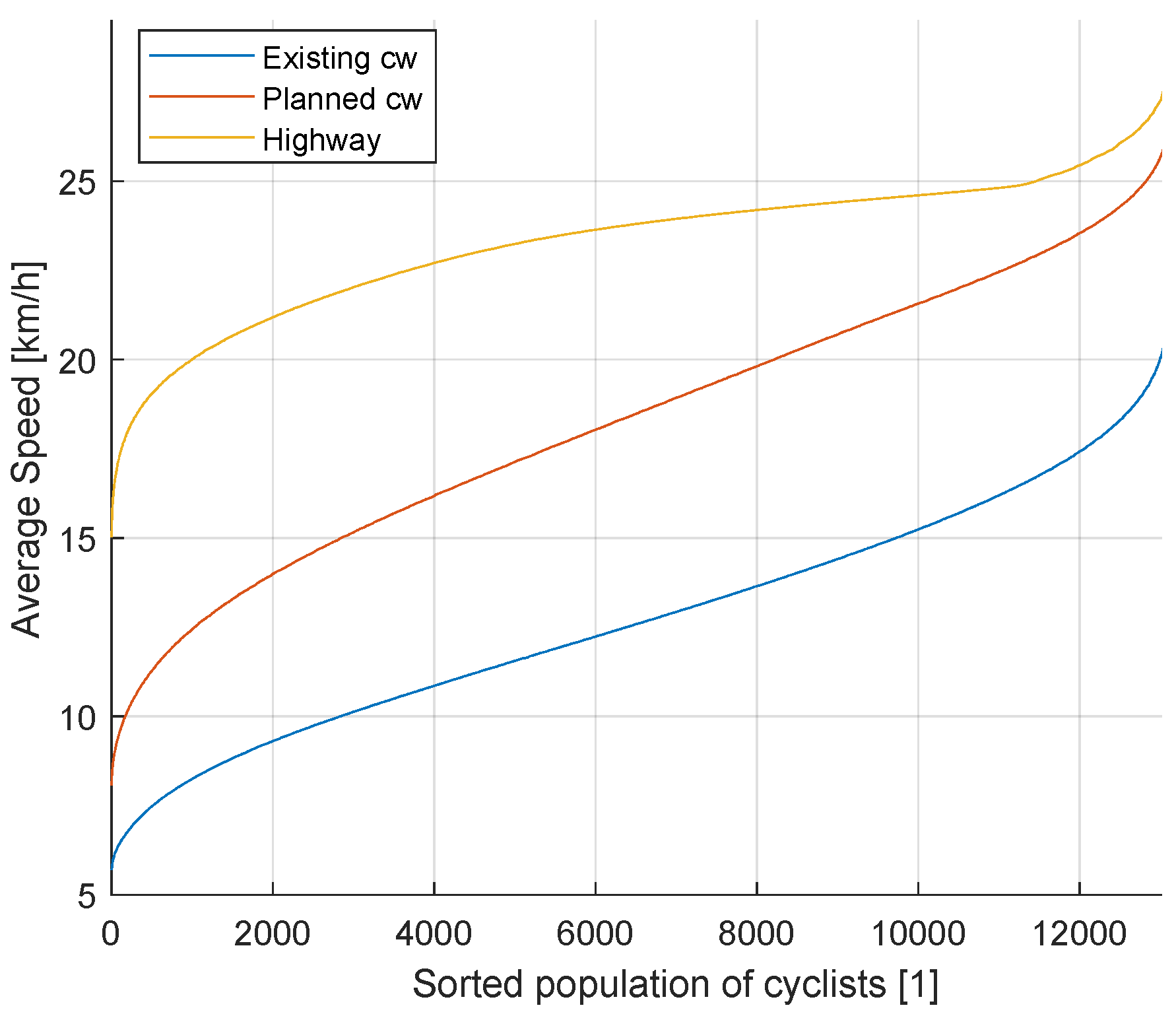
Figure 7.
Travel time distribution of the simulated cyclist population along the three tracks: existing cycleway (blue), planned cycleway (red) and highway (yellow).
Figure 7.
Travel time distribution of the simulated cyclist population along the three tracks: existing cycleway (blue), planned cycleway (red) and highway (yellow).
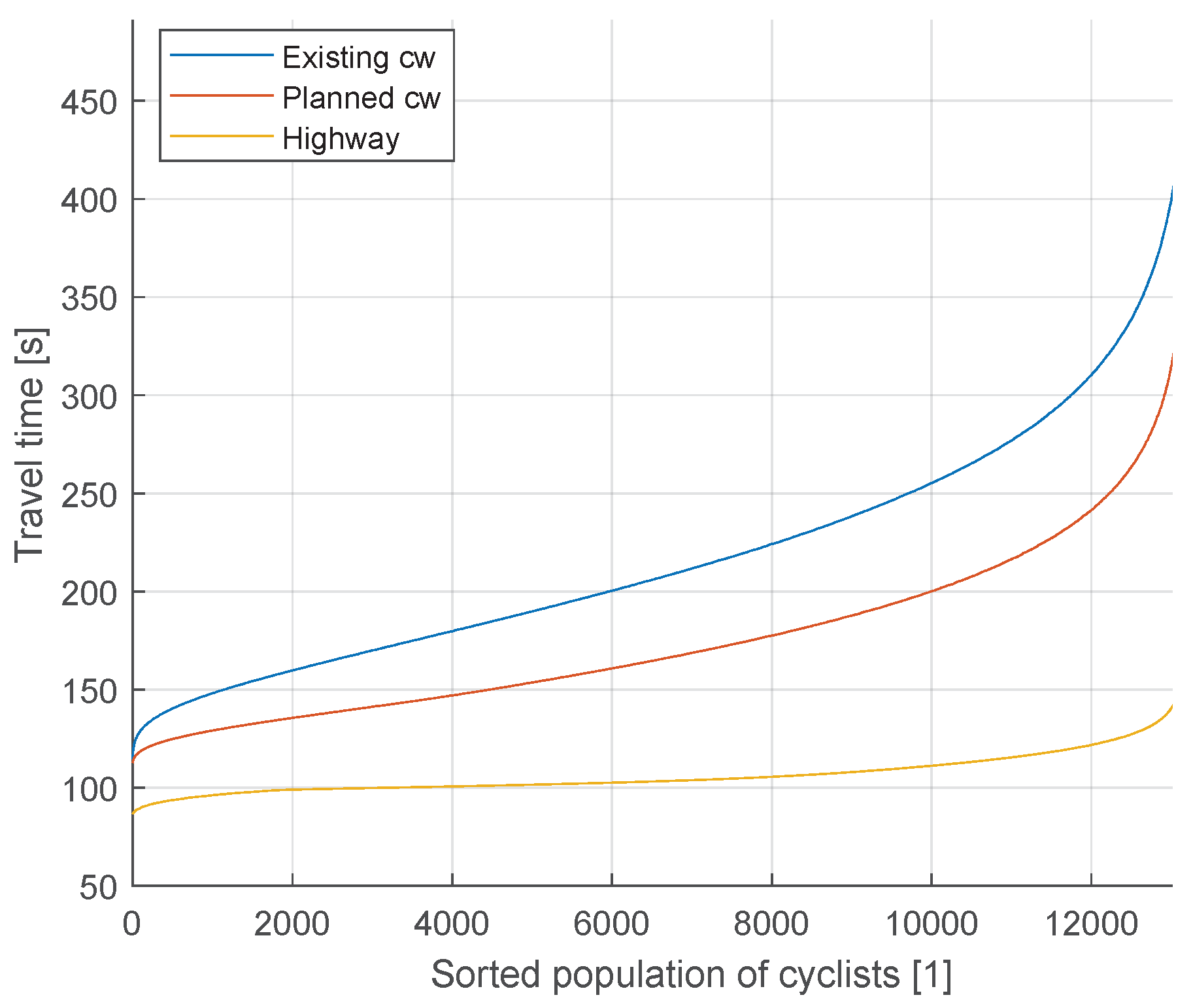

Table 1.
Parameters defining an individual cyclist in the model.
| Parameter | Explanation |
|---|---|
| Constant available power | |
| Short term power (not yet used) | |
| m | System weight |
| A | Frontal area of bicycle and cyclist |
| Aerodynamic drag coefficient | |
| Maximum bicycle speed | |
| Maximum lateral acceleration |
Table 2.
Speed reduction levels.
| Level | Example | |
|---|---|---|
| 1 | free rolling | good sight, cyclist has priority, no traffic expected |
| 2 | good sight, road-users expected who have right-of-way, | |
| or who do not respect the priority | ||
| 3 | bad sight, give way rule or cycle barriers | |
| 4 | Stop-sign / red traffic lights |
Table 3.
Lookup table with factors to adjust the rolling resistance to ambient temperature.
| Temperature | -25°C | -21°C | -17°C | -13°C | -9°C | -5°C | -1°C | 3°C | 7°C | 11°C | 15°C | 19°C | 23°C | 25°C |
|---|---|---|---|---|---|---|---|---|---|---|---|---|---|---|
| Factor | 3.29 | 2.78 | 2.41 | 2.12 | 1.90 | 1.72 | 1.57 | 1.44 | 1.33 | 1.24 | 1.16 | 1.09 | 1.03 | 1 |
14.1cm The coded table covers a range from -25°C to 25°C in 1°C increments. Ambient temperatures below -25°C are not considered with higher factors, while temperatures above 25°C level off to a factor of 1.
Table 4.
Distribution of power (65% of max) spent on utility cycling for people in the age of 20-59 years in deciles.
Table 4.
Distribution of power (65% of max) spent on utility cycling for people in the age of 20-59 years in deciles.
| 10% | 20% | 30% | 40% | 50% | 60% | 70% | 80% | 90% | ||
|---|---|---|---|---|---|---|---|---|---|---|
| Women | 61 | 76 | 85 | 95 | 103 | 112 | 124 | 138 | 162 | W |
| Men | 92 | 111 | 128 | 142 | 156 | 172 | 193 | 213 | 240 | W |
Disclaimer/Publisher’s Note: The statements, opinions and data contained in all publications are solely those of the individual author(s) and contributor(s) and not of MDPI and/or the editor(s). MDPI and/or the editor(s) disclaim responsibility for any injury to people or property resulting from any ideas, methods, instructions or products referred to in the content. |
© 2024 by the authors. Licensee MDPI, Basel, Switzerland. This article is an open access article distributed under the terms and conditions of the Creative Commons Attribution (CC BY) license (http://creativecommons.org/licenses/by/4.0/).
Copyright: This open access article is published under a Creative Commons CC BY 4.0 license, which permit the free download, distribution, and reuse, provided that the author and preprint are cited in any reuse.


