1. Introduction
The primary purpose of measuring the quantity (i.e., mass or volume) and selected gas properties of energy gases is to enable financial transactions between buyer and seller. In this paper, we will call these measurements “fiscal measurements” and the related processes “fiscal metering”. It typically involves the measurement of the flow rate of gas at specified times, and if the transactions are based on energy, the measurement of the calorific value, or more formally, the enthalpy of combustion of the gas passing the sampling point. There are several standards and guidance documents describing fiscal metering of energy-containing gases, e.g., OIML-R140 [
1], EN 1776 [
2] and ISO 15112 [
3]. The models used in these guidelines are very similar, and so are the requirements that measurement equipment shall be calibrated and that measurement results shall be metrologically traceable.
The models used for calculating the volume or energy delivered generally sum the volume or energy increments over time [
3][clause 10]. With regard to the evaluation of measurement uncertainty, usually it is assumed that the quantities of interest (e.g., volume and calorific value) are mutually independent, and essentially normally distributed. Whereas the latter assumption is usually unproblematic, the assumption that the measurement results are mutually independent is only valid under quite peculiar conditions. These conditions include (1) steady-state with respect to flow rate and composition of the gas stream and (2) negligible systematic effects in both the flow meter and the device used for measuring the calorific value (often a gas chromatograph (GC)). Any violation of these conditions will give rise to an increase of the measurement uncertainty.
Steady state conditions with respect to flow rate and composition in gas grids are rare. Due to fluctuations in supply and demand, flow rates differ and the use of different kinds of natural gas give rise to fluctuations in composition. In an era, where gas grids are facing a further diversification of the gas entering into the grid (e.g., biomethane, hydrogen, natural gas import) and the fluctuations also increase, it is obvious that this diversification contributes to an even greater violation of these assumptions. The issue is that the current guidance to some extent acknowledges these issues [
3], but the measurement models and the uncertainty calculations do not take the effects of the practical measurement conditions into account.
In the project called “Metrology for the hydrogen supply chain” (Met4H2) [
4] in the European Partnership of Metrology programme, one objective is devoted to developing
novel methods for the evaluation of measurement uncertainty along the supply chain, namely with regard to the measurement of quantity, and energy and impurity content of hydrogen and hydrogen blends
The associated work is structured to start with natural gas (for which abundant experience and data are available) through hydrogen-enriched natural gas (blends of hydrogen from renewable sources and natural gas) to grids with hydrogen only.
To fully understand this objective, it is important to reiterate that internationally agreed guidance of the evaluation of measurement uncertainty, the Guide to the expression of Uncertainty in Measurement (GUM) requires the evaluation of any covariances between dependent input quantities [
5][clause 5.2]. This evaluation of covariances is perceived by many as difficult, yet it can make the difference between a realistic value for the uncertainty and an unrealistic one [
6]. A realistic value for the uncertainty is required for both gas allocation purposes (i.e., the quantity and energy balance in the grid), as well as to demonstrate conformity with regulatory and contractual requirements.
In this paper, an overview of the ideas behind the envisaged model improvements is given. The overview focusses on three aspects, (a) the effects due to the measurement of the relevant parameters (
Section 2), (b) temporal effects (
Section 3) and (c) the approximation of the total volume, mass, or energy by a summation of increments (
Section 4).
2. Volume, Mass and Energy Measurement
2.1. Framework
The basis for computing the total mass, volume and/or energy is given in ISO 15112 [
3]. For the total mass and volume, the flow rate as a function of the time is the key input. The evaluation of measurement uncertainty is described in several ISO standards [
7,
8,
9,
10]. Such methods for evaluating measurement uncertainty are the fundament for evaluating the measurement uncertainty associated with the total mass or volume of the gas metered.
For the measurement of energy, the calorific value, again measured as a function of time comes into play, supplementary to what was stated previously for measuring the total mass or total volume. The calorific value can be measured directly using a calorimeter or some other inferential device [
11], or by measuring the composition by gas chromatography [
12,
13] followed by a computation of the calorific value using ISO 6976 [
14]. The standards ISO 6974 and ISO 6976 provide the methods for evaluating the measurement uncertainty associated with the calorific value.
There are many possible configurations and approaches to the measurement of energy [
3], but for the modelling it is sufficient to start with a simple configuration. Such a configuration could consist of one flow meter, one temperature transmitter, a pressure transmitter and a gas chromatograph. Such a configuration suffices to outline the relevant improvements to the uncertainty evaluation. Once the methods for obtaining a credible uncertainty statement have been developed for this instance, these methods can be applied to more complex configurations and used in gas networks, for example for gas allocation.
Evaluating dependencies between input quantities in measurement models [
15] is a requirement [
5,
15] and it can make the difference between a credible uncertainty statement and a serious under- or overrating of the measurement uncertainty. The evaluation of correlations in measurements is, for example for measuring the calorific value through GC well established and covered by the relevant standards [
12,
13,
14].
Relative little attention is being paid in the literature to correlations arising from using the same equipment for obtaining a sequence of measurement results. Most examples on uncertainty evaluation [
5,
16,
17,
18,
19] and relevant standards [
7,
8,
9,
10,
12,
13,
14] deal with a single measurement. As the uncertainty budget of a measurement result contains contributions in common with any following measurement result (e.g., from calibration), such results are always mutually correlated. A method for evaluating such correlations is using the uncertainty budgets of a pair of measurement results [
6] which is in turn based on Annex F of JCGM 100 [
5]. From the uncertainty budgets, the variables in common can be identified and these contribute to the covariance between the pair of measurement results.
2.2. Mass
The mass of gas delivered over a time period can be obtained by integrating the mass flow rate as a function of time, viz.,
where
denotes the mass flow rate as a function of time and
and
the end points of the time interval. In practice, this integration is replaced with a summation, i.e.,
where
N denotes the number of mass flow measurements in the time interval
, and it is assumed that the flow rate measurements are made at regular time intervals. Usually, the standard uncertainty of
is obtained using the law of propagation of uncertainty (LPU) for uncorrelated input quantities [
5][eqn. (10)]. If the flow rate measurements are dependent, the standard uncertainty of
can be readily obtained using the LPU for
correlated input quantities [
5][eqn. (13)], or, alternatively, the LPU for multivariate measurement models from JCGM 102 [
18]. The formulation of the LPU in the latter document is already in vector-matrix notation, easing the implementation in computer software. The covariances can be obtained readily from the uncertainty budget for any pair
.
2.3. Volume
The treatment of volume is very similar to that of mass. The gas delivered over a time period can be obtained by integrating the volume flow rate as a function of time, viz.,
where
denotes the volume flow rate as a function of time and
and
the end points of the time interval. In practice, this integration is replaced with a summation, i.e.,
where
N denotes the number of volume flow rate measurements in the time interval
, and it is assumed that the flow rate measurements are made at regular time intervals. The gas volume, as well as the volume flow rate, are pressure- and temperature dependent. In the calculations for volume, the volume flow rate is converted from actual conditions (pressure
p and temperature
T during the measurement) to reference conditions [
20]. These reference conditions differ between countries, but have in common that they are fixed and without uncertainty. The conditions
are measured and hence have uncertainty. The correction factor is given by [
3]
where
Z denotes the compressibility factor. The pressure, temperature and compressibility factor at reference conditions are denoted by the corresponding symbols adorned with a subscript 0. The compressibility factors in equation (
5) are functions of the gas composition [
21,
22]. Usually, different models are used at actual conditions and reference conditions. At reference conditions, often ISO 6976 [
14] is used, whereas at actual conditions equations of state are used like AGA8 [
23,
24] or the GERG-2008 [
22,
25]. Instead of calculation from the gas composition, the compressibility factor can also be obtained from a measured density using the real gas law, provided that the molar mass of the gas is known.
Given the circumstance that the total volume needs to be computed at a single pressure and temperature, which are usually taken as the reference conditions [
3,
20], the propagation of the uncertainty for the total volume is markedly more difficult than for the case of the total mass. On the other hand, applying the LPU to equation (
4) is not much different from that to equation (
2). Only the evaluation of the covariances between pairs of
is more involved, as the covariance arising from the conversion factors from equation (
5) comes into play.
2.4. Energy
The energy of a gas flow is calculated from the basic differential equation [
3]
where
e denotes an energy increment,
H the calorific value and
Q the flow rate of the gas. Equation (
6) underlines that all quantities are functions of time. When using mass flow, the calorific value in equation (
6) is also on a mass basis, and when using volume flow, the calorific value is that of a real gas at volume basis. The reference conditions for the calorific value can be different from those of the flow metering [
14]. Hence, the energy over a time interval
is obtained by integration [
3]
From a physical point of view, it is reasonable to expect that and are continuous functions. Even if for example a rapid change in the gas grid takes place, it takes some time before this change is palpable in full in the measurement results obtained. In reality, flow meters, GCs make measurements at regular time intervals, so all that can be learnt from the functions and are these snapshots.
For the energy determination during 1 , the following two procedures are provided (see also paragraphs 7.2.2.1 and 7.2.2.2 in ISO 15112):
- -
multiplication of the calculated volume under reference conditions with the averaged calculated calorific value of the same hour;
- -
in situ energy calculation in the volume-conversion device using the actual measured entities for the calculation of energy based on the calculation of and , followed by summing these single energy quantities over 1 .
The latter approach approximates the integral in equation (
7) by increments over a period of time
, i.e,
where it is assumed that the uncertainty associated with
is negligible in relation to the uncertainty associated with the summation of the increments.
N denotes the number of increments in the period
.
Using the LPU for uncorrelated input quantities [
5, eqn. (10)],
where the argument
was dropped for brevity. If there only exist correlations among the
and the
separately (so, the covariance between any pair of
would be zero), then the standard uncertainty associated with the energy can be obtained from
At first glance, one might think that equation (
10) addresses all correlations. When realising that the volume flow rate was converted from actual to reference conditions [
20], it becomes apparent that the
in equation (
10) are correlated through the ratio of the compressibility factors
(actual conditions) and
(reference conditions) dependent on the results of the GC analysis, as is the calorific value [
14]. So, the correlation coefficient between
and
would then be non-zero.
3. Temporal Effects
The discussion of the measurement uncertainty so far addressed the uncertainty due to the measurement of flow rates and the calorific value. So, the uncertainty evaluated using equation (
10) only addresses (in part) the measurement. Under steady-state conditions, the uncertainty evaluation presented in
Section 2 may provide a reasonable value for the uncertainty.
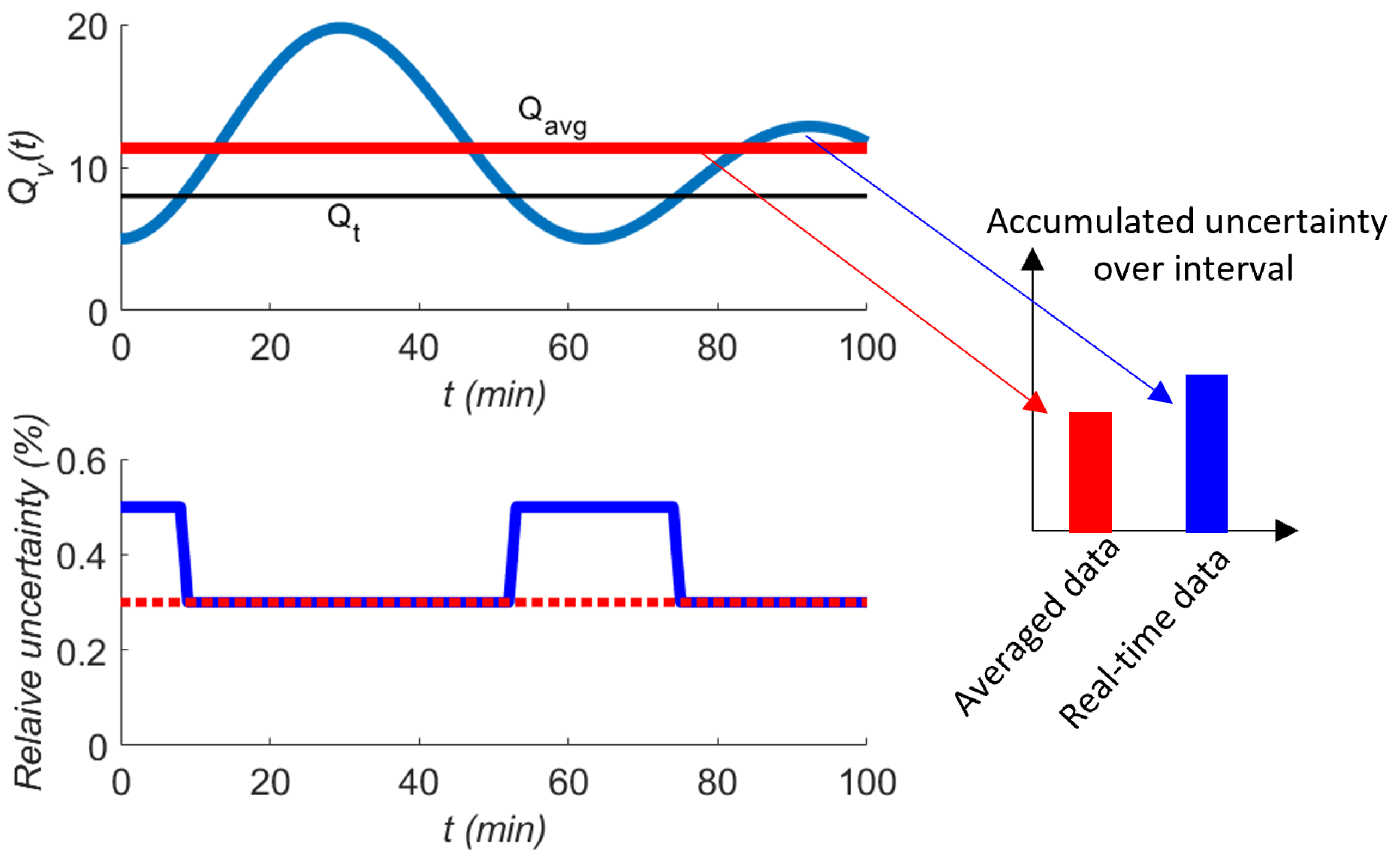
In practice, gas grids are used to support suppliers and users of gas, and notwithstanding that supply and demand are balanced, variations in measured flow rates and calorific values occur. In distribution grids for example, it can be expected that the demand is subject to a day-and-night rhythm, which might look like a sinusoidal signal. This variability should somehow be taken into account, as it affects the mean [
15][clause 11.7] of, say, the flow rate, and by implication thus the total calculated as the sum of the increments (see
Figure 1). The example given in JCGM GUM-6 shows a sinusoidal effect on the temperature of a water bath and the difference in uncertainty using a proper time-series model [
26] and a naive type A evaluation assuming mutual independence of the observations [
5][clause 4.2]. Periodical effects do not only occur in gas networks, but for example also in water networks [
27][example E4.1].
Intuitively, one would expect that the obtained measurement results for flow rates and calorific values become more uncertain with increasing dynamics in fluid flow and diversity of energy gases transmitted or distributed. Also, the magnitude of plays a role here. In a gas grid with dynamics, one would expect that the uncertainty of a calorific value taken as representative for a day to be more uncertain than one taken each 5 min.
Time series models can be fitted using frequentist [
26] and Bayesian methods [
28,
29]. An important aspect in this description of the data is to find an acceptable model for the features in the data. The use of time series analysis may need data driven modelling to be useful. Deliberations such a model choice play then also a role here in the uncertainty evaluation [
15][clause 11.7] as well as model uncertainty [
15].[clause 11.10]
4. Totalisation
Finally, the question arises to what extent the summations in equations (
2), (
4) and (
8) approximate the integrals in equations (
1), (
3) and (
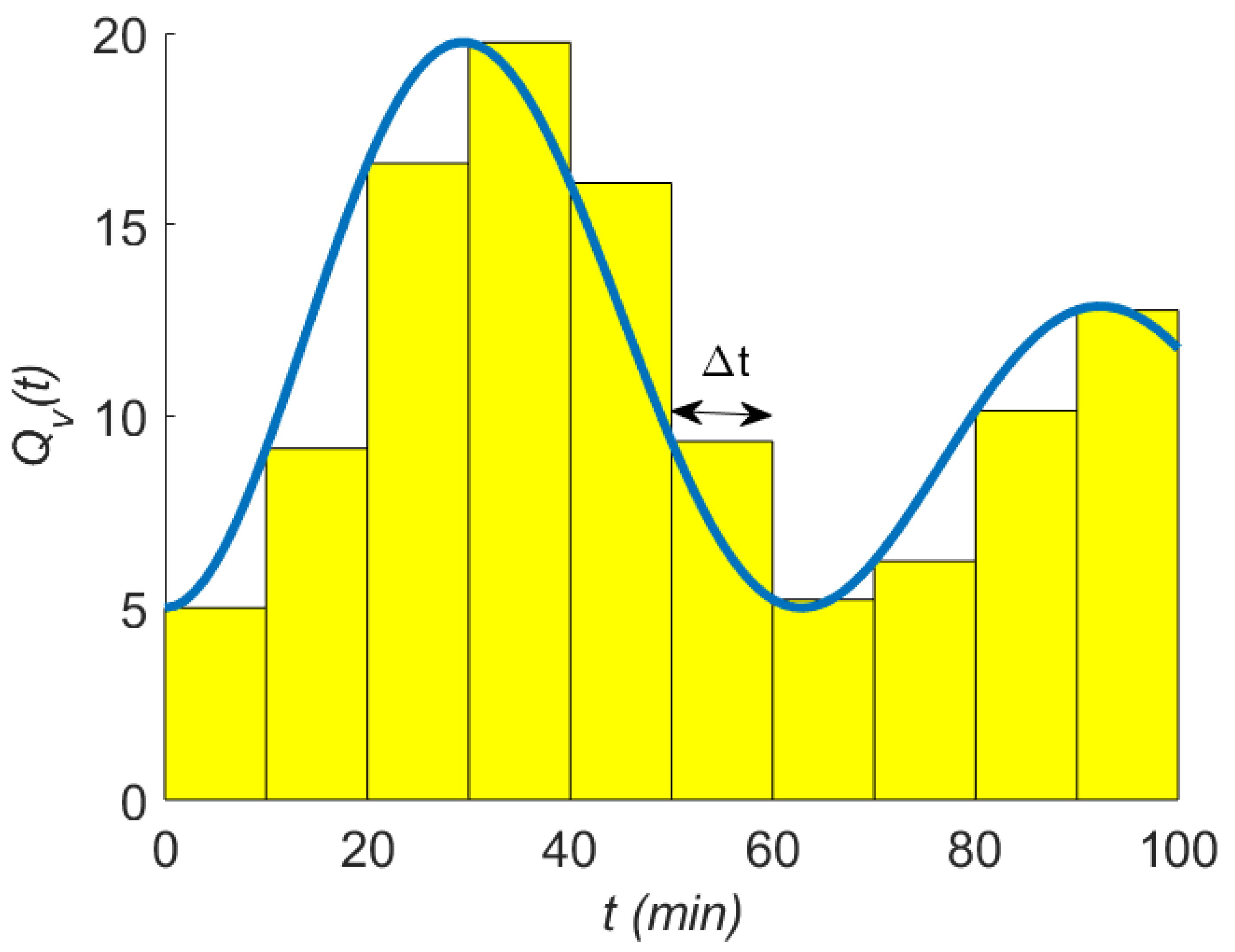
7). The issue is visualised in
Figure 2. The coloured area is the calculated total and the area under the blue curve is the “true” total. In this example, the measurements are taken at time intervals of 10 min. With the same principle, the approximation would be better if the measurements had been taken with a higher frequency, say, every 1 min.
Apart from the time resolution of the measurements, also the dynamics in the grid come into play in this uncertainty component. A measurement result becomes less representative for a time interval if in this interval there are substantial changes in the quantity measured. A practical difficulty can be that one has little clue of such changes (there are no measurements), yet, using the principle of the type B evaluation of measurement uncertainty [
5][clause 4.3], it should be possible to elicit a probability density function (PDF) based on the knowledge at hand. In a gas grid, there are more metering points, and also previous experience can under some circumstances be applied to evaluate the measurement uncertainty arising due to changes in the grid.
For various approaches of numerical integration [
30,
31], the error due to approximation of an integral by a summation is discussed. A practical issue with using these deliberations is that the solid curve in
Figure 2 is not known, so it is not possible to use such approaches to guess the error due to totalisation. Faster, even approximate measurements of the same or related quantities might help in evaluating this uncertainty component.
5. Discussion and Outlook
In this paper, several shortcomings in the current uncertainty evaluation of the total mass, volume and energy in gas grids are presented. Current models and standards assume that the measurement data are independent. Based on simple deliberations, it is shown that this assumption cannot be right. Whereas the uncertainty contributions due to temporal effects and approximating the integral by a summation can be small under steady-state conditions, these uncertainty contributions can be substantial with a greater diversity of gases (e.g., biomethane, hydrogen, natural gas of different origins) in gas grids and with larger fluctuations in supply and demand.
Whereas efforts are made to balance the grid to ensure supply of gas of adequate quality, such efforts cannot make up entirely for the dynamics in the gas grids. In the ongoing transition from fossil natural gas to renewable gases, practices for fiscal metering need urgently to be improved to ensure that these grids can be operated safely and efficiently.
The third shortcoming, the correlation effects between measurement results coming from a single, calibrated instrument are relatively straightforward to capture with the framework of the Guide to the expression of Uncertainty in Measurement. Considering the large volumes of data, the use of vector-matrix algebra as described in JCGM 102 [
18] is commended to obtain compact computer code. This approach has as additional advantage that measurement models can be broken up in parts more freely, as the law of propagation of uncertainty for multivariate measurement models provides by default a full covariance matrix, so that all covariances can be readily propagated from one stage of the measurement model to the next. With the legacy GUM [
5], this is much more difficult, as it presumes that a measurement model can be broken up in expressions with mutually uncorrelated input quantities.
Author Contributions
Conceptualization, AvdV and KF; methodology, AvdV, KF and FG; investigation, AvdV, KF and FG; writing—original draft preparation, AvdV; writing—review and editing, KF and FG; visualization, KF; supervision, AvdV; funding acquisition, AvdV and KF. All authors have read and agreed to the published version of the manuscript.
Funding
The project 21GRD05 Met4H2 has received funding from the European Partnership on Metrology, co-financed from the European Union’s Horizon Europe Research and Innovation Programme and by the Participating States. VSL has received in part funding from the Ministry of Economic Affairs of the Netherlands for this work. The APC was funded by MDPI.
Data Availability Statement
Not applicable.
Conflicts of Interest
The authors declare no conflict of interest. The funders had no role in the design of the study; in the collection, analyses, or interpretation of data; in the writing of the manuscript; or in the decision to publish the results.
Abbreviations
| GC |
gas chromatograph |
| GUM |
Guide to the expression of Uncertainty in Measurement |
| ISO |
International Organisation for Standardisation |
| LPU |
law of propagation of uncertainty |
| MDPI |
Multidisciplinary Digital Publishing Institute |
| PDF |
probability density function |
References
- OIML R 140 Measuring systems for gaseous fuel. OIML, International Organization for Legal Metrology, Paris, France, 2007.
- EN 1776 Gas infrastructure — Gas measuring systems — Functional requirements. CEN, European Committee for Standardization, Brussels, Belgium, 2015. Second edition.
- ISO 15112 Natural gas — Energy determination. ISO, International Organization for Standardization, Geneva, Switzerland, 2011. Second edition.
- van der Veen, A.M.H. Metrology for the hydrogen supply chain. Publishable Summary, EURAMET, Teddington, United Kingdom, 2023. Accessed 2024-08-08.
- BIPM.; IEC.; IFCC.; ILAC.; ISO.; IUPAC.; IUPAP.; OIML. Evaluation of measurement data — Guide to the expression of uncertainty in measurement, JCGM 100:2008, GUM:1995 with minor corrections, 2008.
- Cox, M.G.; van der Veen, A.M.H. Understanding and treating correlated quantities in measurement uncertainty evaluation. In Good Practice in Evaluating Measurement Uncertainty – Compendium of examples, 1st ed.; van der Veen, A.M.H.; Cox, M.G., Eds.; 2021; pp. 29–44.
- ISO 5168 Measurement of fluid flow — Procedures for the evaluation of uncertainties. ISO, International Organization for Standardization, Geneva, Switzerland, 2005. Second edition.
- ISO 5167-1 Measurement of fluid flow by means of pressure differential devices inserted in circular cross-section conduits running full — Part 1: General principles and requirements. ISO, International Organization for Standardization, Geneva, Switzerland, 2022. Third edition.
- ISO 5167-2 Measurement of fluid flow by means of pressure differential devices inserted in circular cross-section conduits running full — Part 2: Orifice plates. ISO, International Organization for Standardization, Geneva, Switzerland, 2022. Third edition.
- ISO 5167-3 Measurement of fluid flow by means of pressure differential devices inserted in circular cross-section conduits running full — Part 3: Nozzles and Venturi nozzles. ISO, International Organization for Standardization, Geneva, Switzerland, 2022. Third edition.
- ISO 15971 Natural gas — Measurement of properties — Calorific value and Wobbe index. ISO, International Organization for Standardization, Geneva, Switzerland, 2008. First edition.
- ISO 6974–1 Natural gas — Determination of composition with defined uncertainty by gas chromatography — Part 1: Guidelines for tailored analysis. ISO, International Organization for Standardization, Geneva, Switzerland, 2012. Second edition.
- ISO 6974–2 Natural gas — Determination of composition with defined uncertainty by gas chromatography — Part 2: Measuring-system characteristics and statistics for processing of data. ISO, International Organization for Standardization, Geneva, Switzerland, 2012. Second edition.
- ISO 6976 Natural gas — Calculation of calorific values, density, relative density and Wobbe indices from composition. ISO, International Organization for Standardization, Geneva, Switzerland, 2016.
- BIPM. ; IEC.; IFCC.; ILAC.; ISO.; IUPAC.; IUPAP.; OIML. Evaluation of measurement data — Guide to the expression of uncertainty in measurement — Part 6: Developing and using measurement models, JCGM GUM-6:2020, 2020. [Google Scholar]
- EA Laboratory Committee. EA 4/02 M Evaluation of the Uncertainty of Measurement In Calibration. European Cooperation for Accreditation, 2022.
- BIPM. ; IEC.; IFCC.; ILAC.; ISO.; IUPAC.; IUPAP.; OIML. Evaluation of measurement data — Guide to the expression of uncertainty in measurement — Supplement 1 to the “Guide to the expression of uncertainty in measurement” — Propagation of distributions using a Monte Carlo method, JCGM 101: 2008, 2008. [Google Scholar]
- BIPM. ; IEC.; IFCC.; ILAC.; ISO.; IUPAC.; IUPAP.; OIML. Evaluation of measurement data — Guide to the expression of uncertainty in measurement — Supplement 2 to the “Guide to the expression of uncertainty in measurement” — Extension to any number of output quantities, JCGM 102: 2011, 2011. [Google Scholar]
- Possolo, A. Simple Guide for Evaluating and Expressing the Uncertainty of NIST Measurement Results. Technical report, 2015. [CrossRef]
- ISO 13443 Natural gas — Standard reference conditions. ISO, International Organization for Standardization, Geneva, Switzerland, 1996.
- ISO 6976 Natural gas — Calculation of calorific values, density, relative density and Wobbe index from composition. ISO, International Organization for Standardization, Geneva, Switzerland, 1995.
- ISO 20765-2 Natural gas — Calculation of thermodynamic properties — Part 2: Single-phase properties (gas, liquid, and dense fluid) for extended ranges of application. ISO, International Organization for Standardization, Geneva, Switzerland, 2008. First edition.
- ISO 12213–1 Natural gas — Calculation of compression factor — Part 1: Introduction and guidelines. ISO, International Organization for Standardization, Geneva, Switzerland, 2006. Second edition.
- ISO 12213–2 Natural gas — Calculation of compression factor — Part 2: Calculation using molar-composition analysis. ISO, International Organization for Standardization, Geneva, Switzerland, 2006. Second edition.
- Kunz, O.; Wagner, W. The GERG-2008 Wide-Range Equation of State for Natural Gases and Other Mixtures: An Expansion of GERG-2004. Journal of Chemical & Engineering Data 2012, 57, 3032–3091. [Google Scholar] [CrossRef]
- Shumway, R.H.; Stoffer, D.S. Time Series Analysis and Its Applications: With R Examples; Springer International Publishing, 2017. [CrossRef]
- A.M.H Van Der Veen.; M.G. Cox.; J. Greenwood.; A. Bošnjakovic.; V. Karahodžic.; S. Martens.; K. Klauenberg.; C. Elster.; S. Demeyer.; N. Fischer.; J.A. Sousa.; O. Pellegrino.; L.L. Martins.; A.S. Ribeiro.; D. Loureiro.; M.C. Almeida.; M.A. Silva.; R. Brito.; A.C. Soares.; K. Shirono.; F. Pennecchi.; P.M. Harris.; S.L.R. Ellison.; F. Rolle.; A. Alard.; T. Caebergs.; B. De Boeck.; J. Pétry.; N. Sebaïhi.; P. Pedone.; F. Manta.; M. Sega.; P.G. Spazzini.; I. De Krom.; M. Singh.; T. Gardiner.; R. Robinson.; T. Smith.; T. Arnold.; M. Reader-Harris.; C. Forsyth.; T. Boussouara.; B. Mickan.; C. Yardin.; M.ˇCauševic.; A. Arduino.; L. Zilberti.; U. Katscher.; J. Neukammer.; S. Cowen.; A. Furtado.; J. Pereira.; E. Batista.; J. Dawkins.; J. Gillespie.; T. Lowe.; W. Ng.; J. Roberts.; M. Griepentrog.; A. Germak.; O. Barroso.; A. Danion.; B. Garrido.; S. Westwood.; A. Carullo.; S. Corbellini.; A. Vallan. Compendium of examples: good practice in evaluating measurement uncertainty, 2020. [CrossRef]
- Gelman, A.; Carlin, J.; Stern, H.; Dunson, D.; Vehtari, A.; Rubin, D. Bayesian Data Analysis, 3rd ed.; Chapman and Hall/CRC: Boca Raton, Florida, USA, 2013. [Google Scholar]
- Stan Development Team. Stan user’s guide. Version 2.30.
- Press, W.H.; Flannery, B.P.; Teukolsky, S.A.; Vetterling, W.T. Numerical Recipes in C: The Art of Scientific Computing, second edition ed.; Cambridge University Press, 1992.
- Mathews, J.H. Numerical methods for mathematics, science, and engineering, 2. ed ed.; Prentice-Hall: Englewood Cliffs, NJ, 1992; 1. Aufl. u.d.T.: Mathews, John H.: Numerical methods for computer science, engineering, and mathematics. - Literaturverz. S. 594 - 603. [Google Scholar]
|
Disclaimer/Publisher’s Note: The statements, opinions and data contained in all publications are solely those of the individual author(s) and contributor(s) and not of MDPI and/or the editor(s). MDPI and/or the editor(s) disclaim responsibility for any injury to people or property resulting from any ideas, methods, instructions or products referred to in the content. |
© 2024 by the authors. Licensee MDPI, Basel, Switzerland. This article is an open access article distributed under the terms and conditions of the Creative Commons Attribution (CC BY) license (http://creativecommons.org/licenses/by/4.0/).