
Submitted:
28 November 2024
Posted:
29 November 2024
You are already at the latest version
Abstract
We investigate the application of deep learning in comparing gait cycle time series from two groups of healthy children, each assessed in different gait laboratories. Both laboratories used similar gait analysis protocols with minimal differences in data collection. Utilizing a ResNet-based deep learning model, we successfully identified the source laboratory of each dataset, achieving high classification accuracy across multiple gait parameters. To address inter-laboratory differences, we explored various preprocessing methods and time series properties that may be detected by the algorithm. We found that standardization of time series values was a successful approach to decrease the ability of the model to distinguish between the two centers. Our findings also reveal that differences in the power spectra and autocorrelation structures of the datasets play a significant role in model performance. Our study emphasizes the importance of standardized protocols and robust data preprocessing to enhance the transferability of machine learning models across clinical settings, particularly for deep learning approaches.
Keywords:
gait
; deep learning
; external validity
; children
1. Introduction
Gait analysis plays a growing role in clinical decision-making in pediatric motor disorders, including diagnostic orientation, disease progression monitoring, and therapeuticdecision support [1]. Children with conditions such as cerebral palsy [2], muscular dystrophies [3], spinal muscular atrophy [4] or pediatric motor disorders [5,6] often exhibit abnormal gait patterns that can be assessed with instrumental gait analysis and in which biomarkers can be extracted [7]. However, despite its clinical value, the widespread application of gait analysis in pediatric clinics is often hindered by the complexity of interpreting high-throughput, multidimensional data. Gait signals—such as joint angles, ground reaction forces, and muscle activations—are typically highly correlated and require expert knowledge for accurate interpretation, making it difficult to fully harness the potential of gait analysis in routine clinical care and clinical research [8].
Machine learning (ML) offers a promising approach to address this challenge. By automating the interpretation of complex data, machine learning models can help reduce the burden on clinicians and make gait analysis easier and faster to interpret [9,10]. In particular, deep learning (DL) has shown potential in processing time-series data such as gait signals, extracting meaningful patterns without needing a priori feature selection [11]. Moreover, DL can easily incorporate complex data from other sources and has interesting properties such as transfer learning, which may be critical to generation models for rare disorders in pediatric neurology [12].
However, a key challenge remains in translating ML models from one clinical setting to another. Gait data collected in different laboratories may differ due to variations in sensor setups, measurement protocols, or participant demographics, complicating the generalization of trained models. Understanding how deep learning models for time-series data perform when comparing similar datasets collected in different laboratories is critical, especially in pediatric populations where precision is essential. This study aims to explore these challenges by comparing gait data from two groups of healthy children, measured in different laboratories, using state-of-the-art deep learning techniques.
2. Methods
2.1. Patients
We included gait data from healthy subjects assessed in two different laboratories. The first group of patients was evaluated in the Central Remedial Clinic in Dublin and included 96 children aged from 4 to 16 years who had been determined as healthy children after careful medical history and examination. The second group of patients was evaluated in the clinical gait analysis laboratory in "Escuela de Fisioterapia de la ONCE-UAM" and formed by 31 children aged from 5 to 15 years who had been considered as healthy children after a systematic medical history and examination. Inclusion criteria were: adequate schooling, absence of any clinical history of neurological, cardiovascular, or systemic diseases, absence of uncorrected visual or hearing impairment, absence of known orthopedic pathologies in the previous six months, and negative results after a screening of unknown orthopedic pathologies through the exploration protocol "Scottish Rite Hospital" [13] and a neurological examination.
2.2. Gait Methods and Laboratories
Gait analysis was performed with a Codamotion system (Charnwood Dynamics Ltd., Rothley, UK). Light emitting markers were attached to reference positions of the subject’s legs, according to an anthropological segment model designed by the manufacturer, and signals were recorded at 200 Hz while the subjects were performing the task. Ground reaction force and inverse kinetic data were obtained from data acquired by a Kitsler power platform, which is also integrated by the manufacturer into the gait system. After initial training, children were incited to walk several times from one end to the other of a long walkway path at their natural, spontaneous speed. Children were asked to repeat the walkway about 8–12 times. The system acquired continuous real-time kinematic data during each complete walk over the walkway. After the acquisition session, individual gait cycles were isolated, by manually marking their beginning (heel contact) and their end (next heel contact of the same foot). Next, each selected cycle was again reviewed to check the consistency of the signal reception. Post-processing was performed with custom-made protocols in the software provided by the gait system manufacturer. For every side gait cycle, we studied the kinematic time series (100-time epochs) of the 3 angular planes (sagittal, horizontal, and coronal planes) from 5 joints (pelvis, hip, knee, ankle, and forefoot). We also studied the mediolateral, anteroposterior, and sagittal ground reaction forces (GRF) and the estimated moment and power time series for the sagittal plane in hip, knee, and ankle joints. For each subject, up to five left and up to five right gait cycles were selected according to technical quality criteria.
Central Remedial Clinic laboratory (Dublin) uses a 14-m long platform, which is placed in a larger room (Figure 1). The gait laboratory in "Escuela Universitaria de Fisioterapia de la ONCE. Universidad Autónoma de Madrid (Figure 2) has a 8-meter long walking platform integrated into a larger room. Space after the platform is smaller, likely provoking that the average walking speed is slower, step cadence is decreased and the stance time is prolonged in Madrid’s healthy children compared to their Dubliners peers (see Table 1)
2.3. Deep Learning Classification Tasks
Many alternative architectures have been presented in the literature in the last decade, proposing different ways of constructing Deep Learning models for the classification of time series. In most cases, these have been adapted from similar problems, e.g. image classification; but are still able to yield excellent results [14], even above those achievable with more traditional approaches [15].
In this work we specifically leverage Residual Networks (ResNet), a type of convolutional neural network architecture introduced to improve the training of deep networks by using skip connections between layers, allowing the network to learn residual functions and address the vanishing gradient problem often encountered in very deep networks [16]. Designed for processing sequential data, ResNet applies convolutional filters along a single dimension to capture local patterns and features effectively. Most importantly, ResNet usually outperforms other DL models, albeit at a higher computational cost [15]. Key hyperparameters in this configuration include the number of residual blocks, set to 5 in this case, with each block consisting of 5 layers that contain 32 filters of size 10.
In order to ensure the generalisability of the results here presented, and exclude their dependence on a specific architecture, some key ones will also be replicated using the following established DL models [14,15]:
- Multi-Layer Perceptrons (MLP) [17]. Basic feedforward neural network composed of two hidden layers of 320 nodes each, all of them fully connected to the units of the next layer.
- Convolutional Neural Networks (CNN) [18]. Basic convolutional architecture, i.e. without layer skipping used in ResNet. We used a configuration with two hidden convolutional layers with 24 filters per layer, with a kernel size of 10 for each filter.
- Transformers [19]. These models are mostly used for processing textual data. They are based on encoding groups of consecutive values into vectors, which are then analyzed by ”attention heads”, or small structures that evaluate the importance of one element with respect to neighboring ones. Key hyperparameters include the number of transformer blocks, the attention head count, and the embedding dimension - all of them set to 4.
- Long Short Term Memory (LSTM) [20]. This is a type of recurrent neural network that is capable of learning long-term dependencies in sequential data, by using memory cells and gating mechanisms to control information flow. We here included two hidden layers of 128 units each, and a drop-out rate of .
Each classification problem here considered starts with a set of time series, representing a specific aspect of the gait along one cycle. An independent ResNet model has been trained on data from the two data sets, with the objective of identifying the source laboratory. In order to simplify the interpretation of results, all classification tasks use the same number of time series for both groups; time series in the over-represented group are selected at random. The performance of the model has then been estimated over a new set of random time series, using the accuracy metric (i.e. fraction of correctly classified time series, here also denoted as “classification score”). To account for the natural stochasticity of the training process, this has been repeated 100 times, with the final classification score corresponding to the median of the individual accuracies.
The data presented in this study are available on request from the corresponding authors. The data are not publicly available due to privacy and ethical restrictions.
3. Results
3.1. Time Series Discrimination
We start the analysis by training DL models using the raw time series recorded by both laboratories, aimed at discriminating (and hence, predicting) the origin of each time series. Figure 3 reports the obtained classification scores, organized by types of signals (see the three colors). Except for the kinematics of the pelvis and hip, the ResNet models can identify the origin laboratory with very high accuracy, in some cases reaching a success. In the knee, ankle, and foot kinematics, although the classification scores were always large, better results were found in the transverse and rotational planes than in the sagittal one. While part of this success is due to the sensitivity of the ResNet model, similar results can be obtained using other (less powerful) DL models, see Figure A1.
We utilized two cross-validation methods—leave-one-cycle-out (LOCO) and leave-one-patient-out (LOPO)—to evaluate the ResNet deep learning model’s generality to classify gait data across different time-series features. LOPO cross-validation selectively assesses the impact on model generalization of inter-subject variability while LOCO does not consider the origin of the variability. Only mild differences in classification scores were found using LOCO and LOPO approaches (see Figure A2). We additionally evaluated whether the differences between the two groups could be due to the resolution of the time series, see Figure A3; while lowering such time resolution can help reduce the classification score, this does not lead to major improvements unless great part of the information is deleted.
To understand what characteristics the DL can be used to discriminate between the two laboratories, we present in Figure 4 an example of a three-time series extracted at random for the moment of the hip, corresponding to Dublin’s (top panel) and Madrid’s (bottom panel) data sets. Two key differences stand out: the initial part of the time series is not similar, with the Madrid’s ones displaying larger fluctuations; and the Madrid’s time series further seem to be more variable and unpredictable, with the presence of high-frequency content.
These major differences can easily be eliminated. On the one hand, the first 30 points of all time series can be deleted (eliminating the first double support and initial part of the single support gait phase), thus only considering the final of them. On the other hand, time series have been smoothed using a Savitzky-Golay filter [21], using a third-order polynomial and a window size of 9 points. Finally, to discard trivial amplitude differences, every time series has been rescaled to have zero mean and unity standard deviation. The time series of both laboratories become much more similar after this processing; see Figure A4 for a graphical representation of the outcome of processing the time series of Figure 4. Despite this, ResNet models trained thereon still achieve a very high classification score, with only minimal decrease across all signals - see black bars of Figure 5 for the reduction in the score, and Figure A5 for full results.
3.2. Differences in Values’ Distributions
As common when dealing with real-world data, the distribution of values in the different time series for both groups of healthy children is not exactly the same. For instance, in Figure A6, we show the particular case of the hip moment time series. To assess whether Resnet could be leveraging these differences in the distribution of time series values, we performed a standardization aimed at deleting the influence of these inherent disparities and obtain a more unified data structure. Specifically, the values of each time series obtained in the previous step (hence of length 70) have been renormalized between zero and one, such that the n-th smallest value is mapped to the value . Note that the result is sets of time series with the exact same value distribution.
This strategy leads to a significant decrease in the accuracy of the models, particularly in those relative to kinematic information (see golden bars of Figure 5 for the reduction in the classification scores). Nevertheless, classification scores remain substantially high ( higher than 0.7 or 0.8) in many time series (Figure A7 for classification scores before and after standardization of time series values).
3.3. Differences in the Auto-Correlation Structure
One of the key elements detected by DL models are local structures of autocorrelation in the time series; to illustrate, the key component of a ResNet model is a convolutional operation, which calculates the presence of short-scale correlations in the data. To check for differences between the time series of both laboratories, Figure A8 reports the median evolution of the autocorrelation of each signal, calculated on the time series modified in the previous step. The global structure is similar in all cases: starting from positive autocorrelations for small values of the lag , the value has a local negative minimum at around , finally converging towards a zero autocorrelation. At the same time, some major differences can be seen near the minimum, both in amplitude and location.
To understand whether these differences are at the basis of the classification performed by the DL models, we plot in Figure 6 three scatter plots, respectively of three metrics as a function of the classification score:
- minima (left panel), i.e. the difference between the corresponding to the minima in both sets of time series. This metric is calculated as , where and are the location of the two minima.
- area (central panel), calculated as the area between both auto-correlation curves.
- Continuous Ordinal Patterns (COP). This is a generalisation of the traditional ordinal pattern approach [22], in which not only the relative order of data points but also their magnitudes is taken into account; and that have proven to be relevant in characterising time series, assessing irreversibility [23], and improving causality tests [24]. More in details, random COPs were applied to the time series, and the difference between the result obtained in each group was measured through a Cohen’s D. The higher this difference, the more the structures of correlations within the time series are different; hence, this metric can be seen as a generalised version of the previous ones.
As can be seen in Figure 6, the higher the difference between the auto-correlation structures, the higher the classification score yielded by the ResNet model - see also the best linear fit and the corresponding p-value in each panel, as well as the Spearman’s rank correlation.
Note that the presence of negative values in the auto-correlation function is a consequence of the oscillatory nature of the movement; something that can easily be spotted in the examples of Figure 4. The changes observed in Figure A8 and validated in Figure 6 thus indicate differences in the amplitude and frequency of such oscillations.
3.4. Differences in Frequency Content
The previous results on the auto-correlation structure of time series also suggest the presence of differences in their frequency content. To test this, the power spectrum of each time series has been estimated using Welch’s method [25]. Compared to other standard approaches (e.g. the Fast Fourier Transform) Welch’s approach yields more stable results, especially in the presence of noise and non-stationarities.
As in the case of autocorrelation, a full depiction of the median power content of all time series is included in Figure A9; on the other hand, Figure 7 provides an overview of the relationships between the obtained classification score, and the maxima (left panel, i.e. the difference between the maxima in the two power spectra) and the area (right panel, difference between the power spectra). A clear relation can be appreciated in the latter case - see linear fit and p-value in the corresponding panel, as well as Spearman’s rank correlation. The spectra’s maxima, on the other hand, seem to yield more limited information; this may nevertheless be caused by the extreme nature of maxima as a parameter and the limited length of the time series, which reduces the available resolution on the spectra themselves. The relationship between the classification scores and the area of the power spectra reveals that the model may be focusing on specific variations and oscillations that are occurring at different frequencies in the two datasets.
3.5. Localisation of Differences
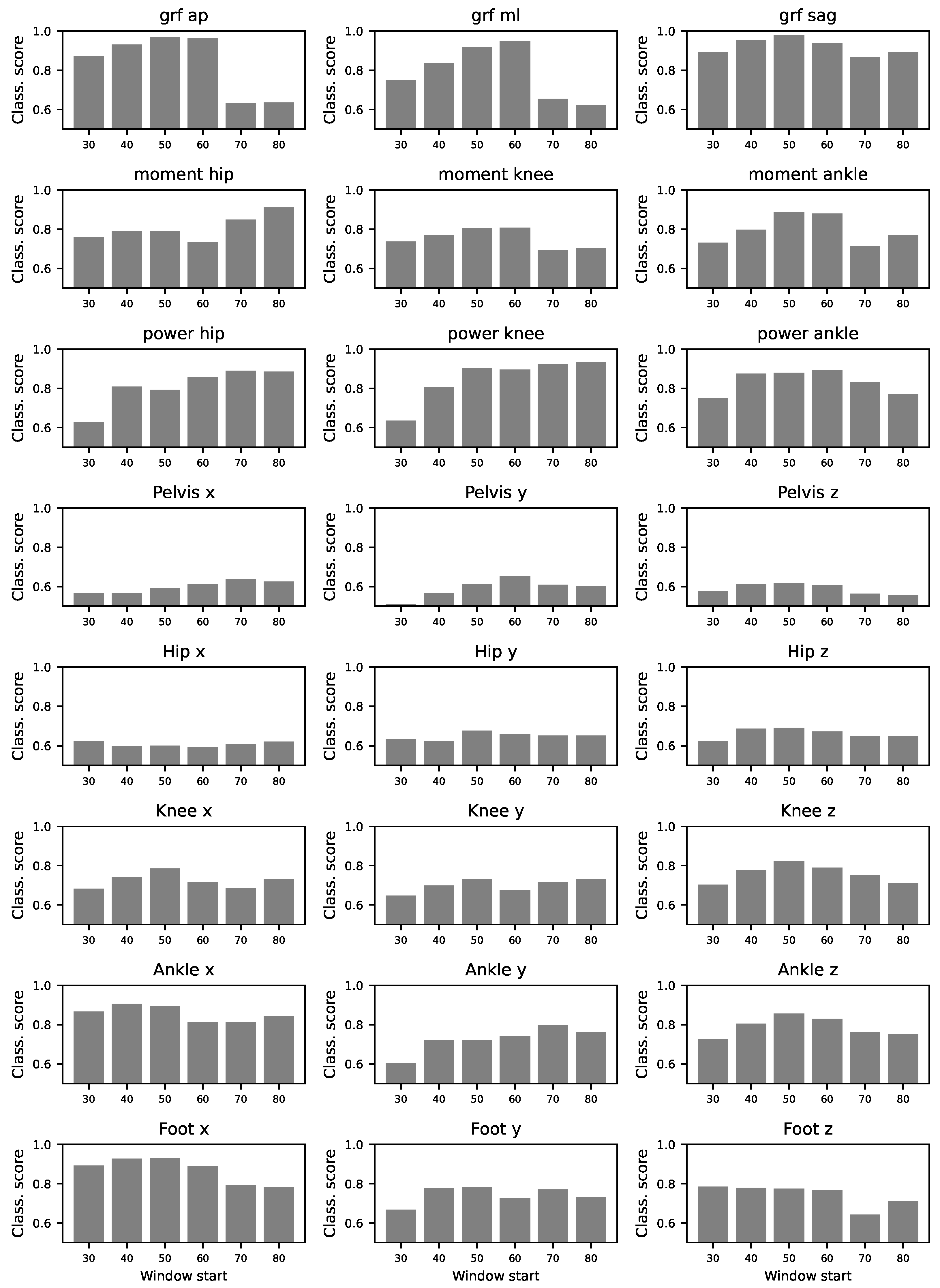
To assess the contribution of different gait cycle segments to classification performance, we divided the time series into sub-windows including information from 20% of the gait cycle. We excluded the first 30% of the gait cycle due to the presence of evidence differences in this portion of the gait cycle. In Figure A10, we show that most of the sub-windows retain significantly high classification scores, comparable to the results of using the whole gait cycle. Figure 8 shows a summary of these results and highlights the sub-windows with higher classification scores. Notice that there is not a predominant section of the gait cycle which may be contributing more to laboratory classification.
4. Discussion and Conclusions
In this study, we demonstrate that deep learning can accurately classify gait data from two samples of healthy children that were evaluated in two different laboratory settings that share equipment and assessment approaches. Even though laboratories share many conditions, ResNet was able to detect the origin of the data with significant accuracy in every time series (see Figure 3), probably based on the combination of small differences. We used different validation procedures and other machine learning approaches with robust (but significantly less accurate) results (see Figure A1). Some differences are easy to spot by just looking at the time series. These include the difference in the initial part of the time series, and the presence of a higher high-frequency noise in one of the datasets (see Figure 4). We eliminate these two aspects yielding minor differences in the classification score, see Figure A5. Lowering the temporal resolution of the time series leads to a reduction in the classification ability, but in contest to our expectation, models’ accuracies remains particularly robust (see Figure A3). This robustness to time series modifications and the superiority against other machine learning algorithms highlights the power of deep learning in detecting laboratory-variant features. As a valid pre-processing approach we studied. the standardization of the distribution of isles in the time series. When time series are modified to have a uniform distribution, classification scores substantially drop, especially for moments and kinematics variables (see Figure A7). Finally, we have shown that the classification score is strongly related to differences in the auto-correlation structures and the power spectra of the signals. Specifically, the former ones seem to indicate that the oscillatory nature of the signal is different in the two laboratories (see Figure A8), and contrary to other differences, this is difficult to reduce through processing after data collection. We also explored the part of the gait cycle that is more relevant for distinguishing between the two laboratories without any clear pattern.
We have recorded two sets of gait data in two laboratories trying to match all conditions as closely as possible. In contrast to our initial expectations, in which a detectable but small difference may be found, the model was able to accurately distinguish between groups. The two laboratories use the same gait system but there are some differences in the space and the floor the children walked. There were also small differences in temperature and illumination. These variations provoked differences in the walking strategy as shown by distinct spatiotemporal parameters but also affected the recording introducing distinct features in the gait signals. We believe that these differences in the spatiotemporal configuration of gait leads to differences in the analysed time series. As the spatiotemporal parameters are different but overlapping between the two healthy datasets, this would be partially explaining the ability of the models to detect differences. Walking speed is the spatiotemporal parameter whose influence on kinematic and kinetic time series has been more studied [26]. For instance, slower speeds typically increase support times and alter muscle activation patterns, as the body adjusts to maintain stability under different constraints. At lower speeds, stance phases dominate, extending the duration of double support phases. This adaptation could result in less dynamic, stability-focused muscle activation, leading to more gradual shifts in joint movements and ground reaction forces. Conversely, as speed increases, stance, and double support times shorten, demanding faster and more intense muscle activations to propel the body forward, changing the timing and intensity of joint power generation [27].
The presence of higher noise at the the beginning of the time series could arise from differences in the gait walkway used by the children such as the elasticity of the platform, distance, and different self-selected walking speeds. Another source of bias may be related to different strategies for selecting valid gait cycles, a process that was done independently in the two centers. We think that the impact of this fact is minimal after sharing the criteria we used and two of the Spanish researchers enjoyed a short research stay in Dublin. Moreover, small differences in signal filtering in the different sensor settings may also contribute to increased interlaboratory differences. Another source of difference between groups could be provoked by different cultural backgrounds [28] and stimuli [29] that the healthy children may have received during acquisitions.
These differences between controls measured at different laboratories impacts the data transferability. We believe that strict standardization of protocols remains critical to eliminate the influence of equipment differences and the walking environment. However, there are some limitations to implement this in real life. One potential solution would be the use of virtual reality or treadmills, but this also modifies gait performance decreasing the natural validity of the studies [30,31]. Another possible measure for easier inter-laboratory transferability of data and models could be the improvement of calibration moving from particular sensors (easy and currently done) into a calibration of the whole system (complex and highly unexplored) [32]. These limits point out the importance of increasing cross-validation studies and the application of data harmonization techniques, which will be more powerful if fed with more lab-to-lab comparisons.
Our results also highlight how complicated can be the translation of models trained in one laboratory or environment into a different one. This limits the deployment of machine learning models in real-world healthcare environments which are critical to provide a more personalized and accurate gait analysis to children and other patients [33,34]. We think that accumulating information about differences between different control datasets coming from different laboratory settings and about how models may detect differences between control groups is one of the first steps to ease the applications of models trained in one or several labs into different ones.
Approaches in pre-processing data (simple as standardization or more complex as data harmonization with autoencoders [35,36]) or evaluating the impact of using laboratory-invariant features in the early part of model development could be developed to overcome this problem [37]. This step allows models to focus more on meaningful gait patterns rather than dataset-specific distinctions, thereby improving generalization and potentially leading to more robust model performance. In our study, we analyzed different approaches. The most successful one was the standardization of the distribution of the time series values. Another promising strategy to address the challenge is transfer learning, a technique where a model trained on one task is adapted to perform on a related task or environment, such as a different laboratory [38].
The observation that differences in the power spectra relate to the performance of the deep learning model suggests that spectral features play a significant role in the model’s ability to distinguish between datasets. The power spectrum of a signal captures how the signal changes are distributed across different frequencies [39]. So, different power spectra imply distinct frequencies in which normal kinematic and kinetic changes occur. This fact can occur due to several reasons, such as differences in sampling rates (not likely in our case), and different sensor noises (maybe related to differences in floor material and/or other conditions in the laboratory), or intrinsic biomechanical differences (for instance, those provoked by different speeds, cadences, and distributions of support and swing time in the gait cycle of the two datasets). When two datasets have different power spectra, this implies differences in the frequency components of gait patterns—possibly due to variations in sampling rates, sensor noise, or intrinsic biomechanical differences. These spectral differences can introduce distinct features or biases that the deep learning model learns to associate with specific datasets.
The combination of two cross-validation approaches is also a relevant contribution to our work. The LOPO cross-validation results reveal a more pronounced challenge in generalizing across different individuals. As expected, the classification scores tend to be lower than those observed in the LOCO setting. This outcome is consistent with the notion that gait patterns can vary significantly between individuals due to factors such as body morphology, walking habits, and subtle differences in movement strategies. The comparison between LOCO and LOPO highlights the strengths and challenges of applying deep learning models to gait analysis. In LOCO, the high classification scores suggest that the ResNet model performs well in capturing intra-subject gait variability which appears to be the most stable and informative. However, in LOPO, where the model is tasked with generalizing across different individuals, we found lower classification scores but cross-validation classification scores remain high. This reveals that ML approach can detect intra-individual variability, but mostly inter-individual variability.
Deep learning has been extensively used in gait analysis [11]. Deep learning approaches have shown that they are able to demonstrate even individual gait patterns and predict identities in healthy subjects [40] or accurately predict kinematic performance under different circumstances [41]. This kind of applications suggest that deep learning could make classifications with small differences in the time series.
Our study has limitations. We have only tested a single deep-learning algorithm. In our experience, ResNet is one of the most powerful available approaches for time series, and the fact that a single model performs in the extremely fine way Resnet performs is already a cause for concern in the application of deep learning models without adequate data harmonization. Moreover, we tested other ML approaches which also show good accuracy for classification. We only included two laboratories, but in that way we were able to compare two laboratories with very similar settings. Even in these circumstances, we were able to find differences. These results highlight the need for studies including more laboratories and different gait analysis systems. Another limitation, which is intrinsic to the use of deep learning approaches, is the problems we have in explaining which features are driving the detection of differences. However, we think that we have explored several explanations.
In conclusion, our study demonstrates that deep learning and other machine learning algorithms can accurately detect differences between two samples of healthy children assessed in two different laboratories. Some pre-processing techniques may reduce the classification ability of the algorithms, and may be important in the transfer of applications for supporting clinical decisions between laboratories.
Author Contributions
Conceptualization, A.G., D.K., J.A.M.G., J.L.L., I.P.V., E.R., M.Z., and D.G.A.; Data curation, A.G., D.K., I.P.V., and D.G.A.; Formal analysis, A.G., E.R., M.Z., and D.G.A.; Funding acquisition, D.K., J.A.M.G., J.L.L., E.R., and M.Z.; Investigation, A.G., D.K., J.A.M.G., J.L.L., I.P.V., and D.G.A.; Methodology, M.Z. and D.G.A.; Resources, D.K., J.A.M.G., J.L.L., E.R., M.Z., and D.G.A.; Software, M.Z.; Validation, E.R., M.Z., and D.G.A.; Writing – original draft, M.Z. and D.G.A.; Writing – review & editing, A.G., D.K., J.A.M.G., J.L.L., I.P.V., E.R., M.Z., and D.G.A.
Funding
This research was funded by Escuela Universitaria de Fisioterapia ONCE-UAM and TACTIC project - FORTALECE ISCIII grant no. FORT23/00034, Grant CNS2023-144775 funded by MICIU/AEI/10.13039/501100011033 by “European Union NextGenerationEU/PRTR”. This project has also received funding from the European Research Council (ERC) under the European Union’s Horizon 2020 research and innovation programme (Grant Agreement No. 851255). This work has been partially supported by the María de Maeztu project CEX2021-001164-M funded by the MCIN/AEI/10.13039/501100011033 and FEDER, EU. This research has been supported by a grant for an international stay from the Universidad Autonoma de Madrid travel grants Program for participation in International Research Conferences.
Acknowledgments
We want to acknowledge families and children for their genereous contribution as controls in both laboratories. We would also like to thank administrative personnel in both laboratories for their helpful support in organization.
Conflicts of Interest
DGA declares the following potential conflicts of interest: Speaker honoraria received from Biogen, PTC, Pfizer, Roche, and Novartis; travel support from Roche, Pfizer, Biogen, and Italfarmaco; advisory roles with Novartis, Pfizer, Roche, Biogen, Sarepta, Audentes, Santhera, and Entrada Tx. The author has participated in clinical trials and other studies sponsored by Biogen, Roche, Novartis, Dyne, Pfizer, Santhera, Fibrogen, UCB Pharma, and Quince Tx. The author holds stocks or stock options in Aura Robotics and UCB Pharma. Research support has been provided by Audentes. IPV is currently an employee of UCB Pharma, which has not intervened in this work. The rest of the authors has no conflict of interest to declare. The funders had no role in the data analysis and writing of this work
Abbreviations
The following abbreviations are used in this manuscript:
| COP | Continuous Ordinal Pattern |
| DL | Deep Learning |
| GRF | Ground Reaction Force |
| LOCO | Leave-One-Cycle-Out |
| LOPO | Leave-One-Patient-Out |
| ML | Machine Learning |
Appendix A
Figure A1.
Classification score obtained with ResNet models benchmarked against Multi-Layer Perceptron (MLP), Convolutional Neural Networks (CNN), Transformers, and Long-Short Term Memory (LSTM) models. Note that ResNet reach larger classification scores in most of the time series. MLP: basic feedforward neural network composed of two hidden layers of 320 nodes each, all of them fully connected to the units of the next layer [17]. CNN: basic convolutional architecture, i.e. without layer skipping used in ResNet. We used a configuration with two hidden convolutional layers with 24 filters per layer, with a kernel size of 10 for each filter [18]. Transformers: Models mostly used for processing textual data, they are based on encoding groups of consecutive values into vectors, which are then analysed by “attention heads”, or small structures that evaluate the importance of one element with respect to neighbouring ones [19]. Key hyperparameters include the number of transformer blocks, the attention head count, and the embedding dimension - all of them set to 4. LSTM: type of recurrent neural network that is capable of learning long-term dependencies in sequential data, by using memory cells and gating mechanisms to control information flow [20]. We here included two hidden layers of 128 units each, and a drop-out rate of .
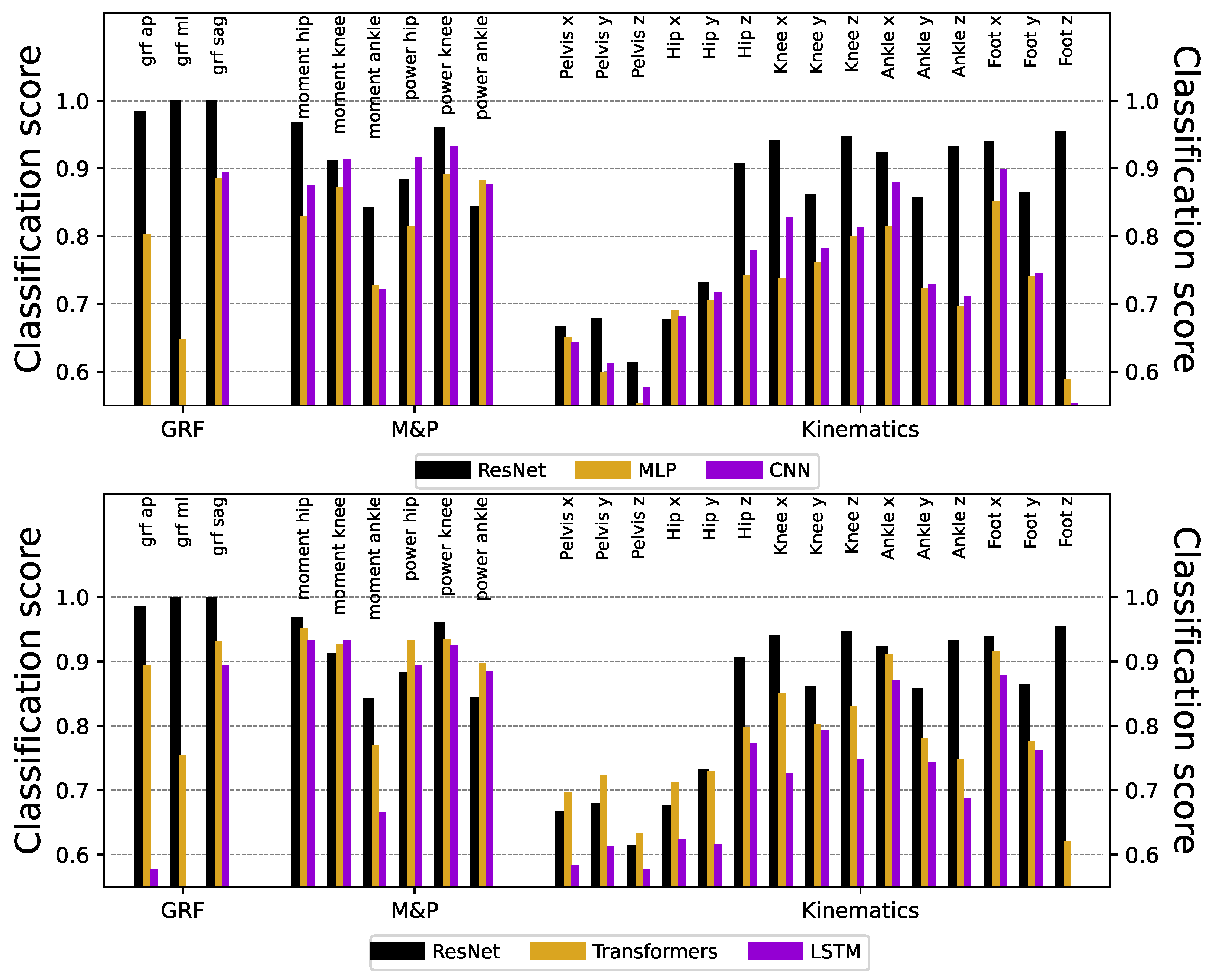
Figure A2.
Classification score obtained with ResNet models, using a two-fold (black bars) and a Leave-One-Patient-Out (golden bars) validation strategies.
Figure A2.
Classification score obtained with ResNet models, using a two-fold (black bars) and a Leave-One-Patient-Out (golden bars) validation strategies.
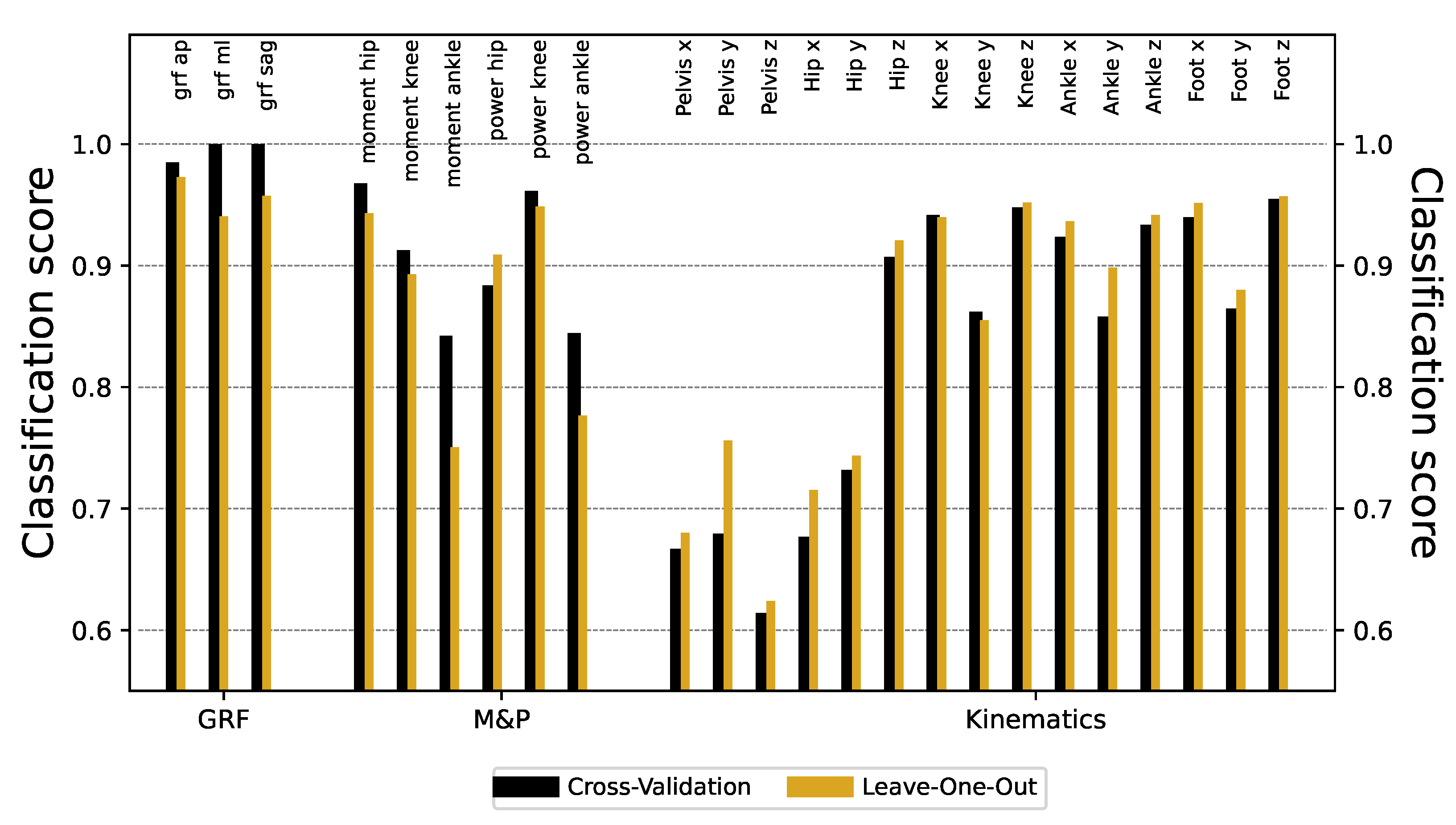
Figure A3.
Median classification score as a function of the length of the considered time series.
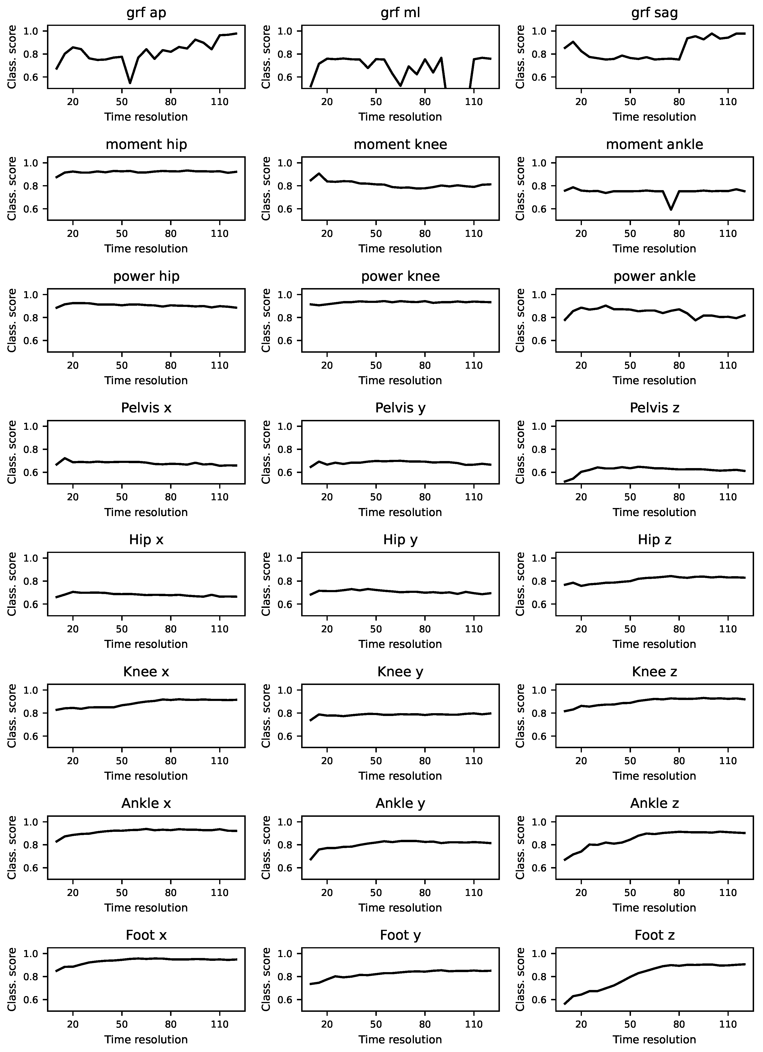
Figure A4.
Graphical representation of the time series shown in Figure 4, after the processing described in Section 3.1 - comprising the deletion of the initial segment, a smoothing using Savitzky-Golay filters, and a rescaling. Time series correspond to Dublin’s (top panel) and Madrid’s (bottom panel) laboratories.
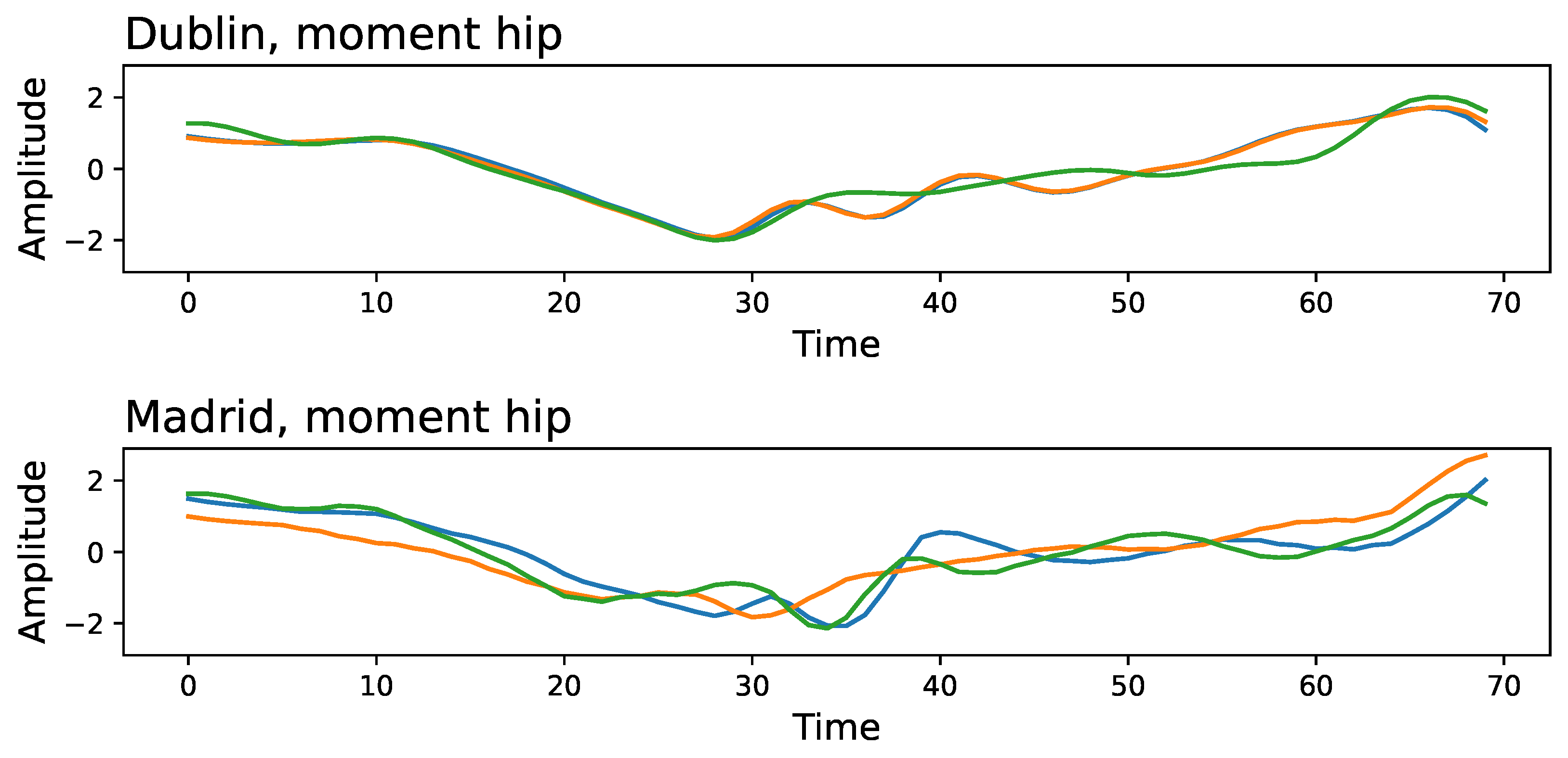
Figure A5.
Classification of modified time series. Black and golden bars depict the classification score obtained by ResNet models for different time series, respectively the raw ones (black) and the one modified as per Section 3.1 (gold).
Figure A5.
Classification of modified time series. Black and golden bars depict the classification score obtained by ResNet models for different time series, respectively the raw ones (black) and the one modified as per Section 3.1 (gold).
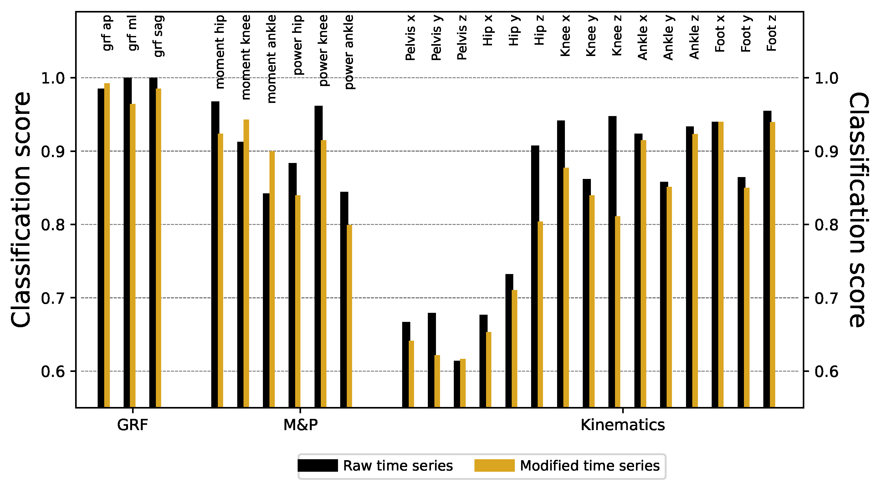
Figure A6.
Modification of the time series’ distributions. Left panels report graphical representations of the time series shown in Figure 4, from Dublin’s (top left panel) and Madrid’s (bottom left panel) laboratories, with their values’ distributions modified according to the procedure described in Section 3.2. Right panels report the density histograms of the time series’ values, before (top right) and after (bottom right) the manipulation, for Dublin’s (black bars) and Madrid’s (golden bars) data sets.
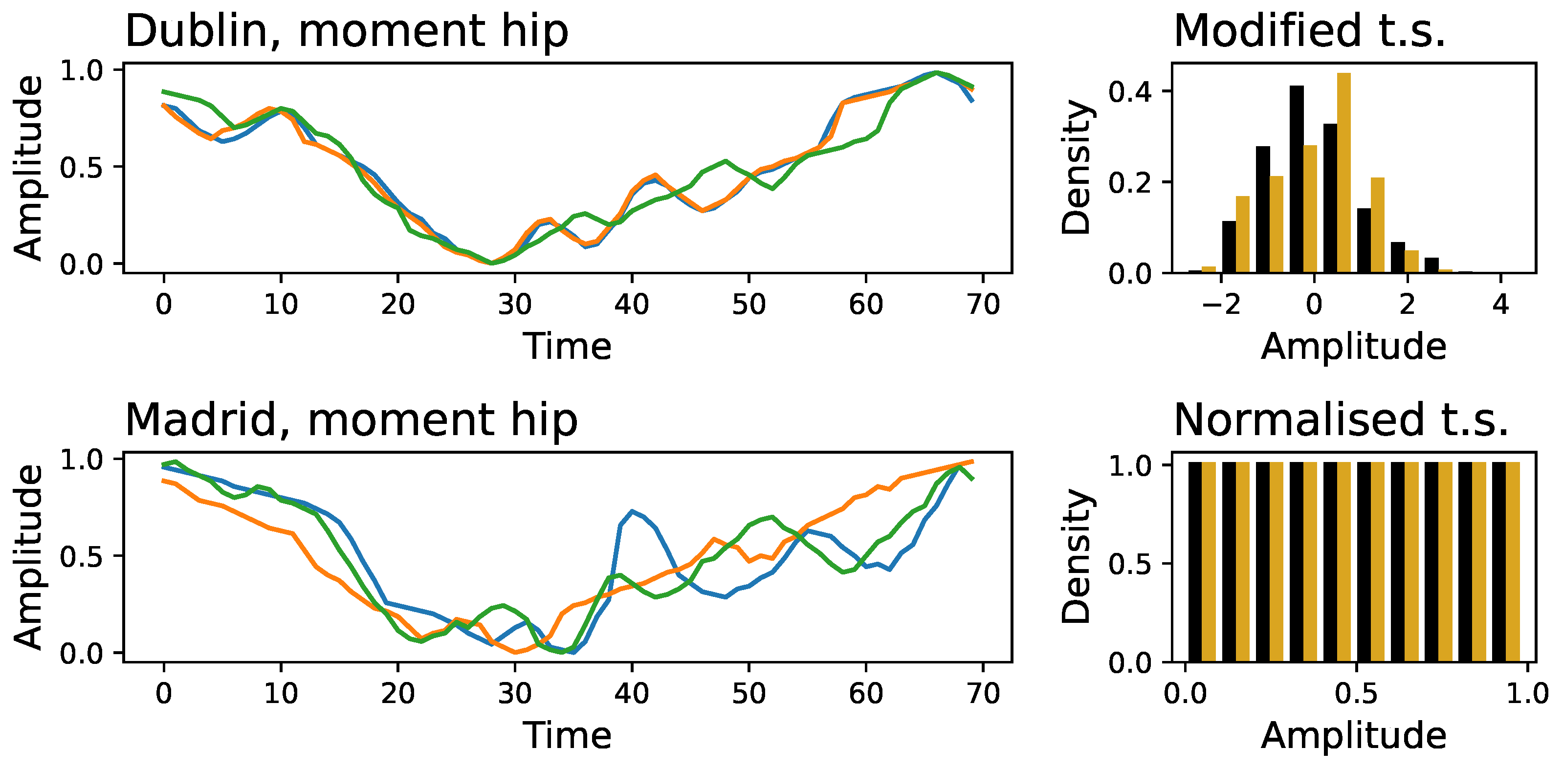
Figure A7.
Classification of time series of modified distributions. Black and golden bars depict the classification score obtained by ResNet models for different time series, respectively the modified ones of Section 3.1 (black bars, corresponding to the golden ones of Figure 3.1) and the ones with their distribution modified as per Section 3.2 (gold).

Figure A8.
Auto-correlation functions for Dublin’s (black) and Madrid’s (red) time series. Lines represent the median calculated across all time series of a single type, while transparent bands the percentiles of the same.
Figure A8.
Auto-correlation functions for Dublin’s (black) and Madrid’s (red) time series. Lines represent the median calculated across all time series of a single type, while transparent bands the percentiles of the same.
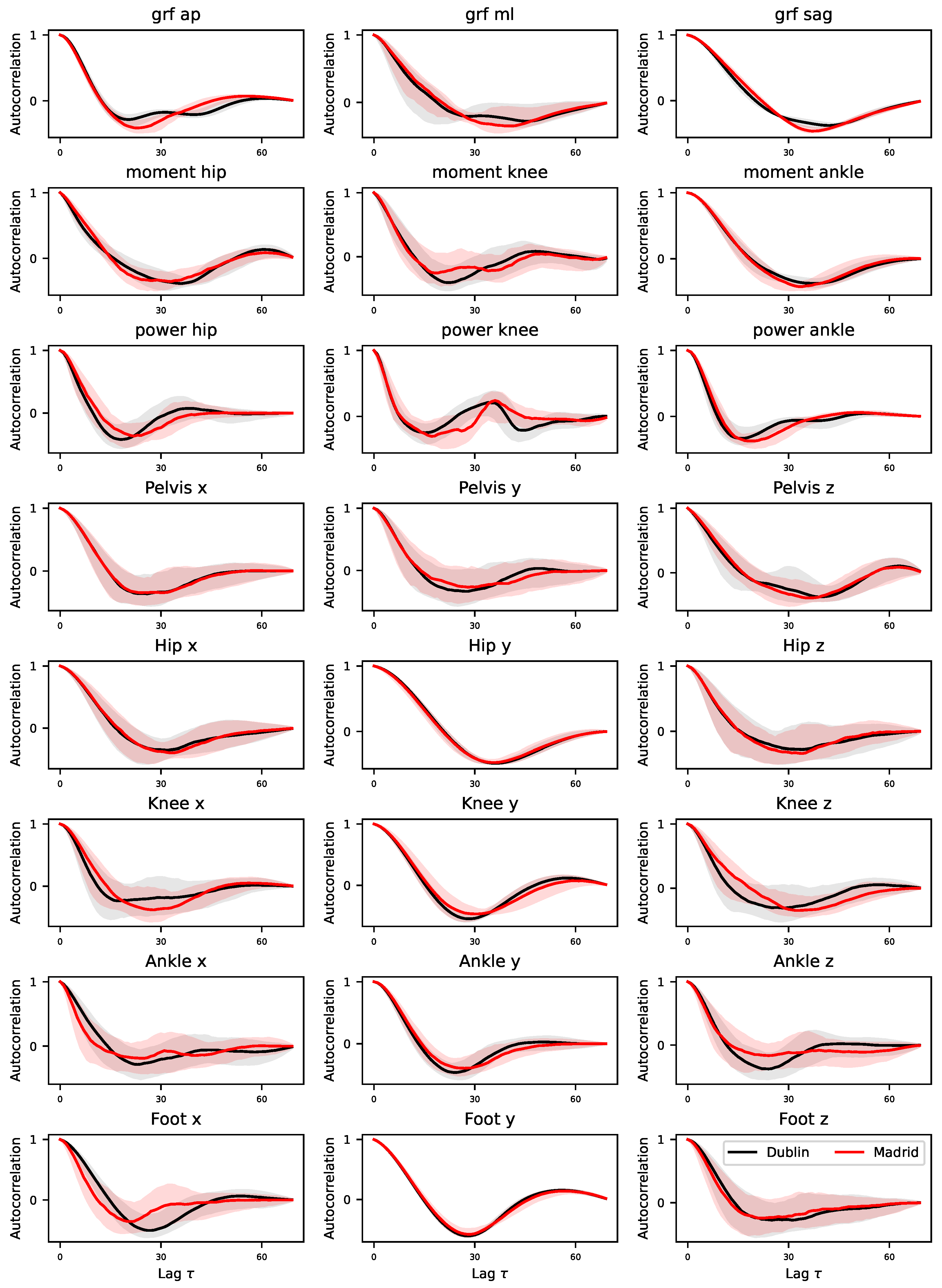
Figure A9.
Power spectra of Dublin’s (black) and Madrid’s (red) time series. Lines represent the median calculated across all time series of a single type, while transparent bands the percentiles of the same. The power spectra have been calculated using the Welch’s method [25], see Section 3.4 for details.
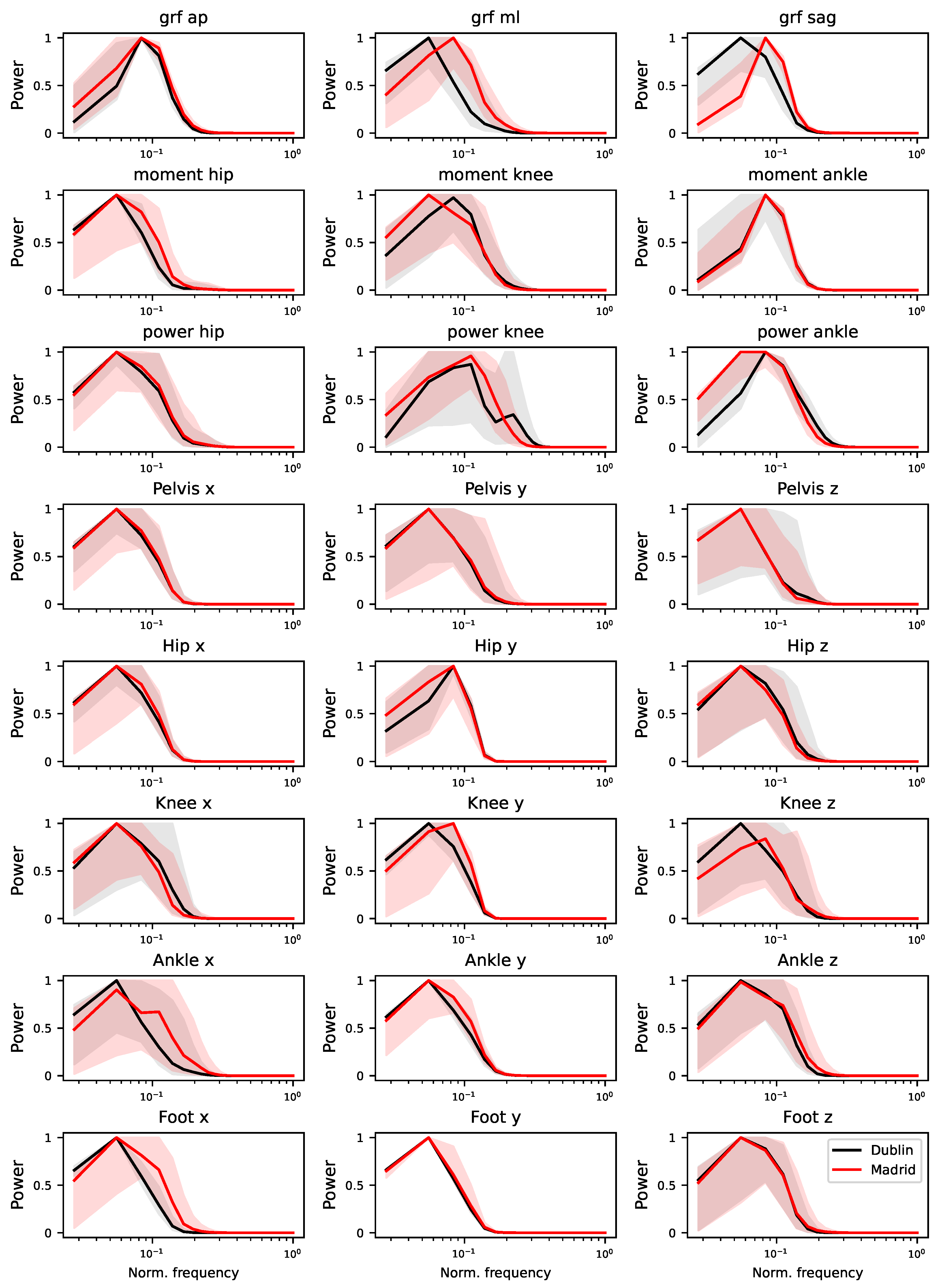
Figure A10.
Relevance of time series’ segments. Each panel reports the classification score obtained by a ResNet model, using sub-windows of the original time series, for the 24 available variables. Each one of these windows starts at the percentage of the gait cycle reported in the X axis, and has a length of 20.
References
- Feng, J.; Wick, J.; Bompiani, E.; Aiona, M. Applications of gait analysis in pediatric orthopaedics. Current orthopaedic practice 2016, 27, 455–464. [Google Scholar] [CrossRef]
- Armand, S.; Decoulon, G.; Bonnefoy-Mazure, A. Gait analysis in children with cerebral palsy. EFORT open reviews 2016, 1, 448–460. [Google Scholar] [CrossRef] [PubMed]
- Goudriaan, M.; Van den Hauwe, M.; Dekeerle, J.; Verhelst, L.; Molenaers, G.; Goemans, N.; Desloovere, K. Gait deviations in Duchenne muscular dystrophy—Part 1. A systematic review. Gait & posture 2018, 62, 247–261. [Google Scholar]
- Kennedy, R.A.; Carroll, K.; McGinley, J.L.; Paterson, K.L. Walking and weakness in children: a narrative review of gait and functional ambulation in paediatric neuromuscular disease. Journal of foot and ankle research 2020, 13, 1–15. [Google Scholar] [CrossRef] [PubMed]
- Faccioli, S.; Cavalagli, A.; Falocci, N.; Mangano, G.; Sanfilippo, I.; Sassi, S. Gait analysis patterns and rehabilitative interventions to improve gait in persons with hereditary spastic paraplegia: a systematic review and meta-analysis. Frontiers in Neurology 2023, 14, 1256392. [Google Scholar] [CrossRef]
- Vasco, G.; Gazzellini, S.; Petrarca, M.; Lispi, M.L.; Pisano, A.; Zazza, M.; Della Bella, G.; Castelli, E.; Bertini, E. Functional and gait assessment in children and adolescents affected by Friedreich’s ataxia: a one-year longitudinal study. PloS one 2016, 11, e0162463. [Google Scholar] [CrossRef] [PubMed]
- Ilg, W.; Milne, S.; Schmitz-Hübsch, T.; Alcock, L.; Beichert, L.; Bertini, E.; Mohamed Ibrahim, N.; Dawes, H.; Gomez, C.M.; Hanagasi, H.; et al. Quantitative gait and balance outcomes for ataxia trials: consensus recommendations by the ataxia global initiative working group on digital-motor biomarkers. The Cerebellum 2024, 23, 1566–1592. [Google Scholar] [CrossRef]
- Marin, J.; Marin, J.J.; Blanco, T.; de la Torre, J.; Salcedo, I.; Martitegui, E. Is my patient improving? Individualized gait analysis in rehabilitation. Applied Sciences 2020, 10, 8558. [Google Scholar] [CrossRef]
- Halilaj, E.; Rajagopal, A.; Fiterau, M.; Hicks, J.L.; Hastie, T.J.; Delp, S.L. Machine learning in human movement biomechanics: Best practices, common pitfalls, and new opportunities. Journal of biomechanics 2018, 81, 1–11. [Google Scholar] [CrossRef]
- Özateş, M.E.; Yaman, A.; Salami, F.; Campos, S.; Wolf, S.I.; Schneider, U. Identification and interpretation of gait analysis features and foot conditions by explainable AI. Scientific Reports 2024, 14, 5998. [Google Scholar] [CrossRef] [PubMed]
- Khan, A.; Galarraga, O.; Garcia-Salicetti, S.; Vigneron, V. Deep Learning for Quantified Gait Analysis: A Systematic Literature Review. IEEE Access 2024. [Google Scholar] [CrossRef]
- Banerjee, J.; Taroni, J.N.; Allaway, R.J.; Prasad, D.V.; Guinney, J.; Greene, C. Machine learning in rare disease. Nature Methods 2023, 20, 803–814. [Google Scholar] [CrossRef] [PubMed]
- Herring, J.A. Texas Scottish rite hospital for children. Tachdjian’s Pediatric Orthopaedics, 2008.
- Ismail Fawaz, H.; Forestier, G.; Weber, J.; Idoumghar, L.; Muller, P.A. Deep learning for time series classification: a review. Data mining and knowledge discovery 2019, 33, 917–963. [Google Scholar] [CrossRef]
- Crespo-Otero, A.; Esteve, P.; Zanin, M. Deep Learning models for the analysis of time series: A practical introduction for the statistical physics practitioner. Chaos, Solitons & Fractals 2024, 187, 115359. [Google Scholar]
- Simonyan, K.; Zisserman, A. Very deep convolutional networks for large-scale image recognition. arXiv preprint arXiv:1409.1556, 2014; arXiv:1409.1556 2014. [Google Scholar]
- Wang, Z.; Yan, W.; Oates, T. Time series classification from scratch with deep neural networks: A strong baseline. 2017 International joint conference on neural networks (IJCNN). IEEE, 2017, pp. 1578–1585.
- Zhao, B.; Lu, H.; Chen, S.; Liu, J.; Wu, D. Convolutional neural networks for time series classification. Journal of systems engineering and electronics 2017, 28, 162–169. [Google Scholar] [CrossRef]
- Vaswani, A.; Shazeer, N.; Parmar, N.; Uszkoreit, J.; Jones, L.; Gomez, A.N.; Kaiser, Ł.; Polosukhin, I. Attention is all you need. Advances in neural information processing systems 2017, 30. [Google Scholar]
- Karim, F.; Majumdar, S.; Darabi, H.; Chen, S. LSTM fully convolutional networks for time series classification. IEEE access 2017, 6, 1662–1669. [Google Scholar] [CrossRef]
- Savitzky, A.; Golay, M.J. Smoothing and differentiation of data by simplified least squares procedures. Analytical chemistry 1964, 36, 1627–1639. [Google Scholar] [CrossRef]
- Bandt, C.; Pompe, B. Permutation entropy: a natural complexity measure for time series. Physical review letters 2002, 88, 174102. [Google Scholar] [CrossRef]
- Zanin, M. Continuous ordinal patterns: Creating a bridge between ordinal analysis and deep learning. Chaos: An Interdisciplinary Journal of Nonlinear Science 2023, 33. [Google Scholar] [CrossRef]
- Zanin, M. Augmenting granger causality through continuous ordinal patterns. Communications in Nonlinear Science and Numerical Simulation 2024, 128, 107606. [Google Scholar] [CrossRef]
- Welch, P. The use of fast Fourier transform for the estimation of power spectra: a method based on time averaging over short, modified periodograms. IEEE Transactions on audio and electroacoustics 1967, 15, 70–73. [Google Scholar] [CrossRef]
- Fukuchi, C.A.; Fukuchi, R.K.; Duarte, M. Effects of walking speed on gait biomechanics in healthy participants: a systematic review and meta-analysis. Systematic reviews 2019, 8, 1–11. [Google Scholar] [CrossRef]
- Schwartz, M.H.; Rozumalski, A.; Trost, J.P. The effect of walking speed on the gait of typically developing children. Journal of biomechanics 2008, 41, 1639–1650. [Google Scholar] [CrossRef] [PubMed]
- Thevenon, A.; Gabrielli, F.; Lepvrier, J.; Faupin, A.; Allart, E.; Tiffreau, V.; Wieczorek, V. Collection of normative data for spatial and temporal gait parameters in a sample of French children aged between 6 and 12. Annals of Physical and Rehabilitation Medicine 2015, 58, 139–144. [Google Scholar] [CrossRef]
- Brinkerhoff, S.A.; Murrah, W.M.; Hutchison, Z.; Miller, M.; Roper, J.A. Words matter: instructions dictate “self-selected” walking speed in young adults. Gait & Posture 2022, 95, 223–226. [Google Scholar]
- Hollman, J.H.; Watkins, M.K.; Imhoff, A.C.; Braun, C.E.; Akervik, K.A.; Ness, D.K. A comparison of variability in spatiotemporal gait parameters between treadmill and overground walking conditions. Gait and Posture 2016, 43, 204–209. [Google Scholar] [CrossRef]
- Janeh, O.; Langbehn, E.; Steinicke, F.; Bruder, G.; Gulberti, A.; Poetter-Nerger, M. Walking in Virtual Reality: Effects of Manipulated Visual Self-Motion on Walking Biomechanics. ACM Trans. Appl. Percept. 2017, 14. [Google Scholar] [CrossRef]
- Baker, R. Gait analysis methods in rehabilitation. Journal of neuroengineering and rehabilitation 2006, 3, 1–10. [Google Scholar] [CrossRef] [PubMed]
- Figueiredo, J.; Santos, C.P.; Moreno, J.C. Automatic recognition of gait patterns in human motor disorders using machine learning: A review. Medical engineering & physics 2018, 53, 1–12. [Google Scholar]
- Rehman, R.Z.U.; Del Din, S.; Guan, Y.; Yarnall, A.J.; Shi, J.Q.; Rochester, L. Selecting Clinically Relevant Gait Characteristics for Classification of Early Parkinson’s Disease: A Comprehensive Machine Learning Approach. Scientific Reports 2019, 9, 17269. [Google Scholar] [CrossRef] [PubMed]
- An, Lijun and Chen, Jianzhong and Chen, Pansheng and Zhang, Chen and He, Tong and Chen, Christopher and Zhou, Juan Helen and Yeo, BT Thomas and of Aging, Lifestyle Study and Alzheimer’s Disease Neuroimaging Initiative and others. Goal-specific brain MRI harmonization. Neuroimage 2022, 263, 119570.
- Pomponio, R.; Erus, G.; Habes, M.; Doshi, J.; Srinivasan, D.; Mamourian, E.; Bashyam, V.; Nasrallah, I.M.; Satterthwaite, T.D.; Fan, Y.; et al. Harmonization of large MRI datasets for the analysis of brain imaging patterns throughout the lifespan. NeuroImage 2020, 208, 116450. [Google Scholar] [CrossRef] [PubMed]
- Farahani, A.; Voghoei, S.; Rasheed, K.; Arabnia, H.R. A brief review of domain adaptation. Advances in data science and information engineering: proceedings from ICDATA 2020 and IKE 2020 2021, pp. 877–894.
- Weber, M.; Auch, M.; Doblander, C.; Mandl, P.; Jacobsen, H.A. Transfer learning with time series data: a systematic mapping study. Ieee Access 2021, 9, 165409–165432. [Google Scholar] [CrossRef]
- Skiadopoulos, A.; Stergiou, N. Power spectrum and filtering. In Biomechanics and gait analysis; Elsevier, 2020; pp. 99–148.
- Horst, F.; Lapuschkin, S.; Samek, W.; Müller, K.R.; Schöllhorn, W.I. Explaining the unique nature of individual gait patterns with deep learning. Scientific reports 2019, 9, 2391. [Google Scholar] [CrossRef]
- Semwal, V.B.; Jain, R.; Maheshwari, P.; Khatwani, S. Gait reference trajectory generation at different walking speeds using LSTM and CNN. Multimedia Tools and Applications 2023, 82, 33401–33419. [Google Scholar] [CrossRef]
Figure 1.
Image of the CRC gait laboratory in Dublin.

Figure 2.
Image of gait laboratory in Escuela de Fisioterapia de la ONCE (Madrid).
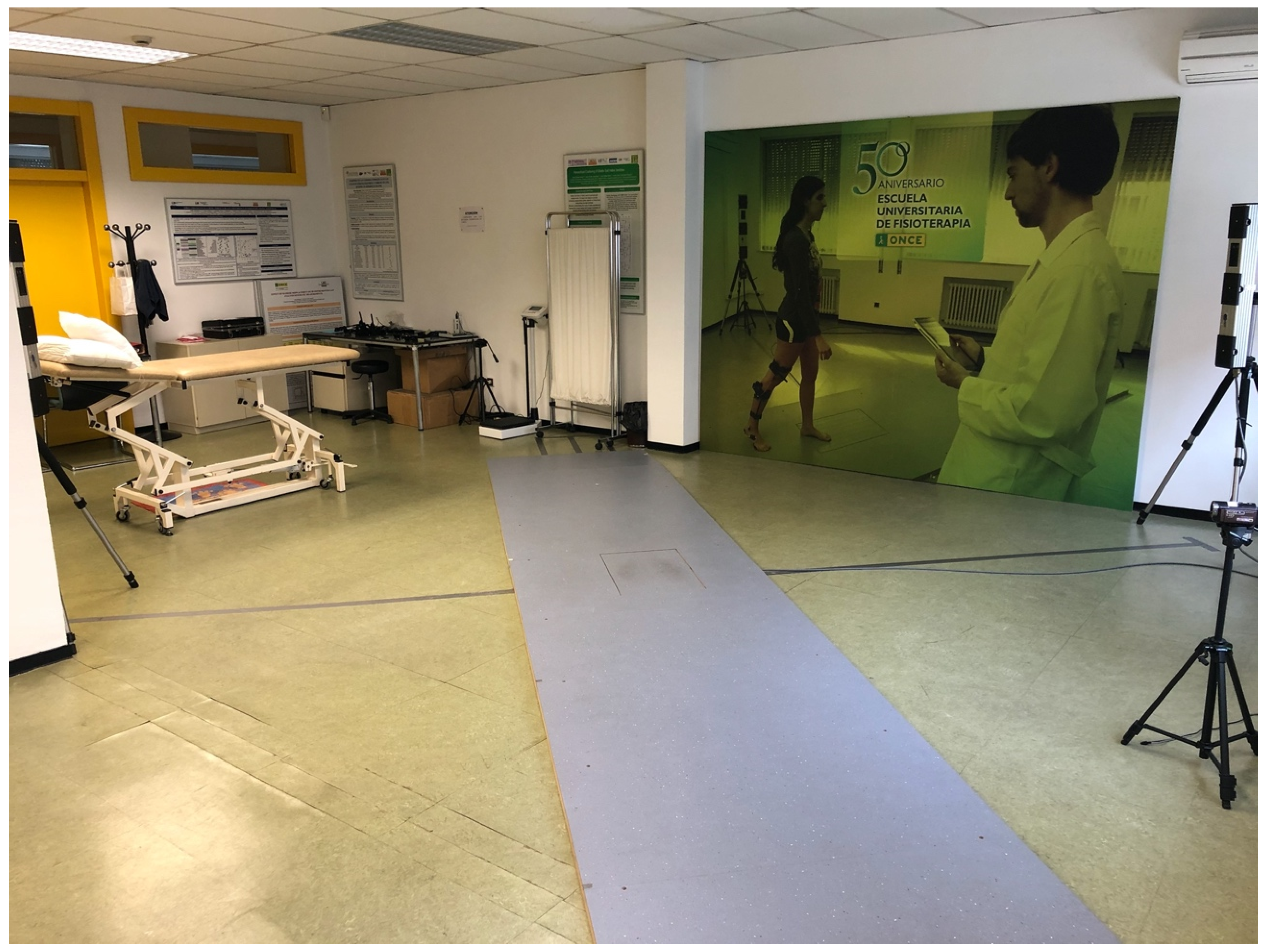
Figure 3.
Classification scores obtained from the raw time series. Scores have been obtained using ResNet models, and correspond to the median over 100 independent realizations.
Figure 3.
Classification scores obtained from the raw time series. Scores have been obtained using ResNet models, and correspond to the median over 100 independent realizations.
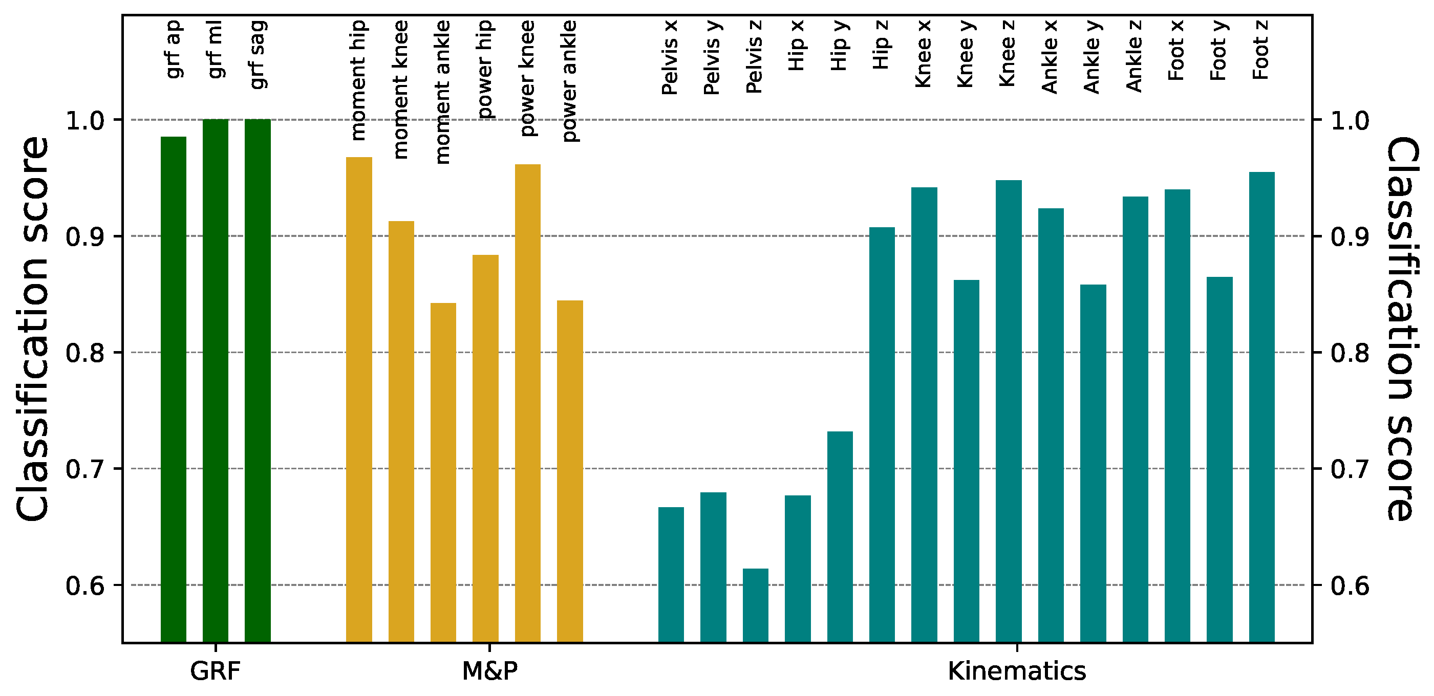
Figure 4.
Three examples of time series, corresponding to the moment of the hip of three different subjects, as recorded in Dublin (top panel) and Madrid (bottom panel).
Figure 4.
Three examples of time series, corresponding to the moment of the hip of three different subjects, as recorded in Dublin (top panel) and Madrid (bottom panel).

Figure 5.
Changes in the classification score of time series under different modifications. Black and golden bars depict the drop observed using ResNet models for different time series, respectively when considering the modified ones of Section 3.1 (black bars), and the ones with their distribution modified as per Section 3.2 (golden bars). For full results, see Figure A5 and Figure A7.
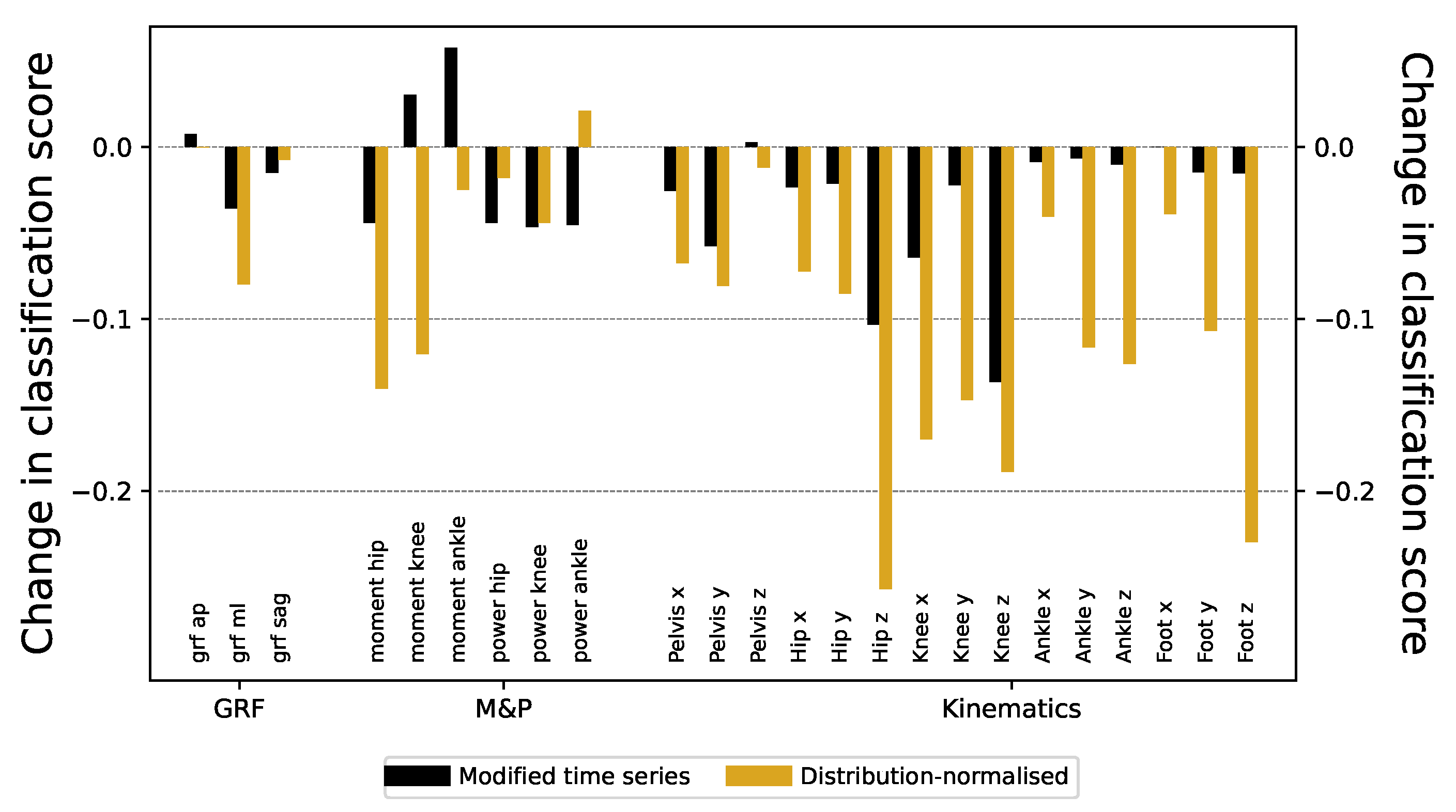
Figure 6.
Analysis of the auto-correlation structure of time series. Left and center panels respectively report the minima and the area as a function of the classification score. The right panel reports the evolution of the COP as a function of the same score - see main text, Section 3.3 for definitions. See also Figure A8 for full results.
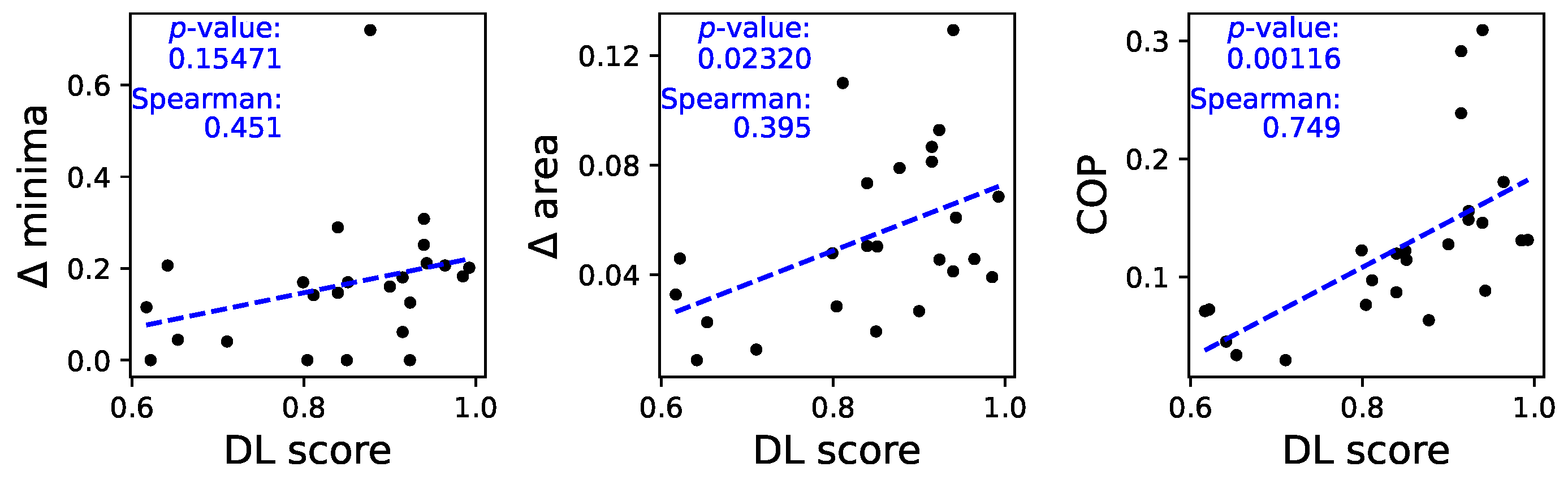
Figure 7.
Analysis of the power spectrum of time series. Left and right panels respectively report the maxima and the area as a function of the classification score - see main text, Section 3.4 for definitions. See Figure A9 for full spectra.
Figure 7.
Analysis of the power spectrum of time series. Left and right panels respectively report the maxima and the area as a function of the classification score - see main text, Section 3.4 for definitions. See Figure A9 for full spectra.
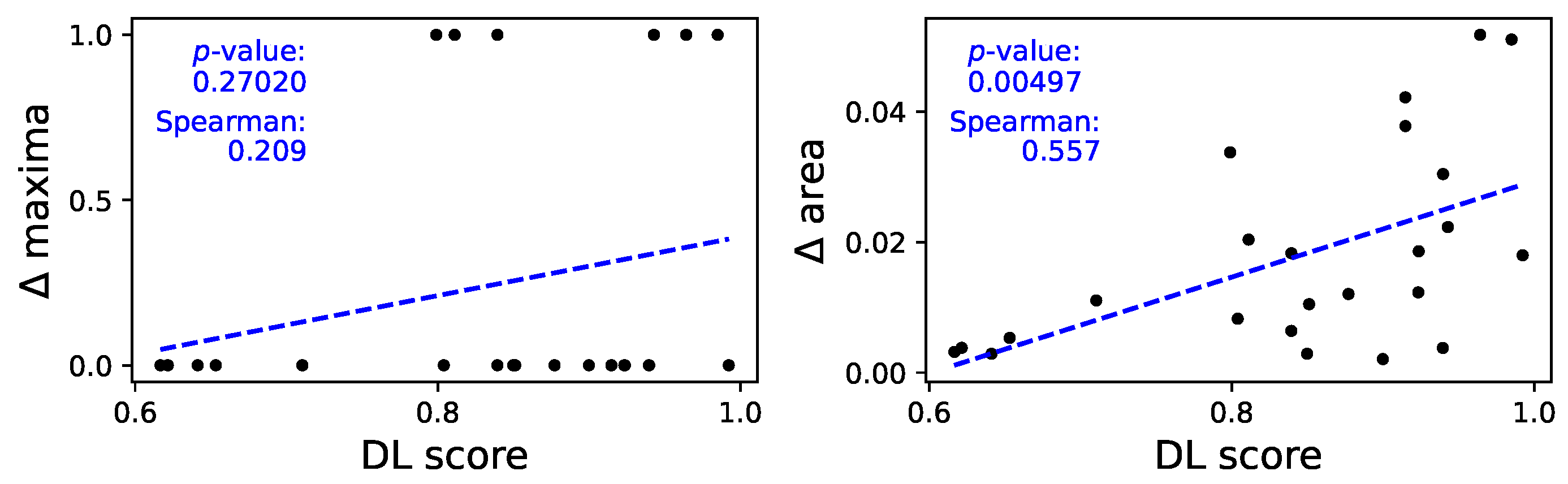
Figure 8.
Relevance of different parts of the time series. Each bar reports in black the location of the segment that allows to obtain the best classification score, using a ResNet model. See Figure A10 for full results. The grey part corresponds to the initial of the time series that is discarded in the filtering described in Section 3.1.
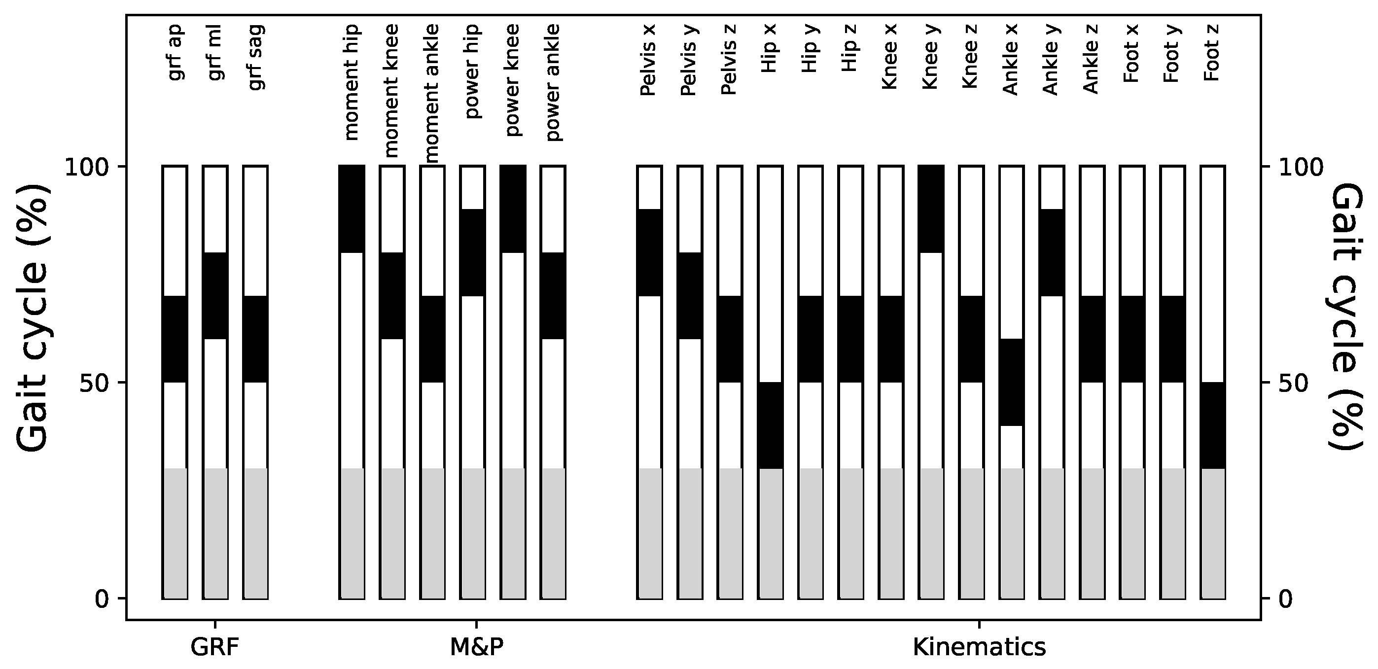

Table 1.
Demographic features and spatiotemporal Gait Features for healthy children assessed in Dublin and Madrid laboratory.
Table 1.
Demographic features and spatiotemporal Gait Features for healthy children assessed in Dublin and Madrid laboratory.
| Feature | Dublin children (N=96) | Madrid children (N=31) |
|---|---|---|
| Sex (Female/Male) | 48F(50%)/48M(50%) | 12F(39%)/19M(61%) |
| Age (years, median [min, max]) | 9.00 [4.00, 16.00] | 9.00 [5.00, 16.00] |
| Weight (kg, median [min, max]) | 31.3 [14.6, 94.7] | 28.6 [18.5, 75.3] |
| Height (cm, median [min, max]) | 1.37 [1.05, 1.83] | 1.38 [1.00, 1.82] |
| Norm. Walking Speed (s−1, median [min, max]) | 1.74 [1.16, 2.44] | 1.49 [1.15, 2.03] |
| Cadence (steps/s, median [min, max]) | 2.18 [1.70, 2.95] | 1.92 [1.56, 2.73] |
| Stance Time (% of gait cycle, median [min, max]) | 61.2 [57.8, 66.7] | 63.3 [60.2, 66.8] |
Disclaimer/Publisher’s Note: The statements, opinions and data contained in all publications are solely those of the individual author(s) and contributor(s) and not of MDPI and/or the editor(s). MDPI and/or the editor(s) disclaim responsibility for any injury to people or property resulting from any ideas, methods, instructions or products referred to in the content. |
© 2024 by the authors. Licensee MDPI, Basel, Switzerland. This article is an open access article distributed under the terms and conditions of the Creative Commons Attribution (CC BY) license (http://creativecommons.org/licenses/by/4.0/).
Copyright: This open access article is published under a Creative Commons CC BY 4.0 license, which permit the free download, distribution, and reuse, provided that the author and preprint are cited in any reuse.


