
Submitted:
25 November 2024
Posted:
26 November 2024
You are already at the latest version
Abstract
We used otolith chemistry tools to test and complement current hypotheses about habitat use and connectivity between Dissostichus mawsoni sub-populations in CCAMLR area 48. Sagittal otoliths from 45 fish sampled around the South Orkney Islands were analysed. Their elemental (Li, Na, Mg, Cr, Mn, Sr, Sn, and Ba, relative to Ca) and isotopic (δ18O and δ13C) signatures were examined in both nuclear and marginal regions, representing juvenile and adult stages, respectively. Potential nursery habitats were geo-located by comparing observed and expected δ18O values. Chemical differences between nuclear and marginal regions were indicative of ontogenetic displacements to deeper offshore habitats, suggesting a discrete habitat shift between 11 and 13 years-old. Data supported the existence of two nursery origins contributing to the study area population. Nonetheless, the location of these origins was unclear and didn not provide any direct support to the hypotheses being currently considered by CCAMLR. Thus, the location and connectivity between nursery and adult habitats, as well as their spawning site fidelity, need to be assessed before disregarding alternative hypotheses07160260Citation: To be added by editorial staff during production. Academic Editor: Firstname Lastname Received: date Revised: date Accepted: date Published: date Copyright: © 2024 by the authors. Submitted for possible open access publication under the terms and conditions of the Creative Commons Attribution (CC BY) license (https://creativecommons.org/licenses/by/4.0/).Citation: To be added by editorial staff during production. Academic Editor: Firstname Lastname Received: date Revised: date Accepted: date Published: date Copyright: © 2024 by the authors. Submitted for possible open access publication under the terms and conditions of the Creative Commons Attribution (CC BY) license (https://creativecommons.org/licenses/by/4.0/)..
Keywords:
Antarctic toothfish
; nursery areas
; demographic units
; otolith chemistry
; stock identification
; stable isotopes
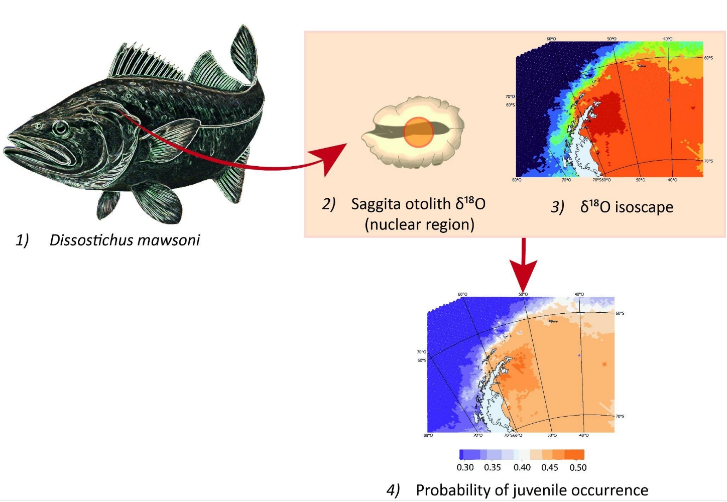
Graphical Abstract
1. Introduction
The Antarctic toothfish Dissostichus mawsoni is a benthopelagic member of the family Nototheniidae, which presents a circumpolar distribution, mainly south of 57°S and closely related to the Antarctic Convergence [1,2]. With a median age and size at first maturity of 13-16 years-old and ~100 cm total length (TL), respectively, its lifespan reaches 50 years, exceeding 200 cm TL and 100 kg of individual mass [3,4]. Several ontogenetic habitat shifts occur during this long lifespan [5,6]. While young-of-the-year (YOY) and yearlings (4-12 cm TL) use shallow pelagic waters close to the coast, older juveniles (19–54 cm TL) become benthic and spend a number of years on the continental shelf at depths between 50 and 300 m [7,8,9]. Subadults (50-95 cm TL) move then to greater depths (500-850 m) on the continental slope [10]. After reaching sexual maturity (~100 cm TL), adults become neutrally buoyant [5,11,12], and expand their bathymetric range greatly, feeding between 10 and 2200 m, although showing some preference for depths between 300 and 500 m [2,13,14].
Dissostichus mawsoni supports one of the two most valuable commercial fisheries in the Southern Ocean, largely in international waters managed by the Commission for the Conservation of Antarctic Marine Living Resources (CCAMLR). CCAMLR jurisdiction is divided into Areas, Sub-areas and Small-Scale Research Units (SSRUs; Figure 1), which are expected to share relatively similar oceanographic and biological characteristics, and to contain relatively discrete populations of some target species [15]. For some others, these CCAMLR divisions may not represent biologically relevant (evolutionary or demographic) units, leading to potentially important mismatches between biology and management actions [16,17]. In the particular case of D. mawsoni, both the number and distribution of evolutionary and demographic units across the Southern Ocean and the degree of matching between these units and CCAMLR areas or sub-areas are poorly known. This uncertainty and incomplete knowledge about the structure, connectivity and dynamics of D. mawsoni demographic units have become core issues in recent critics to CCAMLR regulations, considered too risky given several key parameters of the stock assessment model [18], estimated considering, almost exclusively, biological and fishery data from sub-area 88.1, remain unknown and/or very uncertain [19].
The limited knowledge of D. mawsoni evolutionary units results not only from the small number of studies conducted to date but also from variability in sampling designs, study areas, and molecular techniques [20,21,22]. Tagging studies have shown that while most marked adults remained for years within 50 km of their tagging sites, a few others moved up to 2300 km away [7,23]. Despite its low frequency, these movements could be enough to obscure or cancel out ongoing genetic differentiation processes across very extensive areas [24], biasing the estimation and/or leading to the actual existence of a rather small number of evolutionary units. Nonetheless, the dominance of a resident behavior suggests the existence of separate D. mawsoni demographic units, isolated enough to exhibit asynchronous population dynamics and different life-history parameters [16].
Despite its practical relevance for management purposes, unveiling the number, distribution, and connectivity between D. mawsoni demographic units (i.e. stocks) has received little attention so far [23,25,26], focused on sub-areas 88.1 and 88.2, which concentrates most of the current fishing activity. Here, evidence from otolith chemistry, tagging, biological, fishing, and particle dispersal studies have shaped the current working hypothesis that a single demographic unit exists in these two sub-areas [7,27]. A second demographic unit would exist, nonetheless, west of the Antarctic Peninsula [25,26]. No available studies have been devoted explicitly to scrutinize the structure of demographic units within other areas or sub-areas. This is the case of area 48, which goes from the Antarctic Peninsula to Prince Edward and Marion Islands (Figure 1), and represented 14% of the fishery catch in 2018. Given the overexploitation of several stocks, most of this area has remained closed to all finfish fisheries since 1990 [28].
While fishery-dependent data is scarce after years of fishing closure, fishery-independent information is also very limited for D. mawsoni in Area 48 [29]. Nonetheless, After significant efforts, these authors have proposed three main hypotheses about the structure and connectivity of D. mawsoni demographic units in this area: i) a single demographic unit exhibiting some limited connectivity with area 58 (Indian Ocean sector), ii) two separate units, both placed within the Wedell Sea, with origins in sub-areas 48.2 y 48.6, and iii) at least three interconnected demographic units, with origins in sub-areas 48.1, 48.2, and 48.6 and some limited connectivity with area 58. In the present work, we confront these three hypotheses against otolith chemistry data collected around the South Orkney Island (sub-area 48.2) during exceptional exploratory activities authorized in 2016 and 2018.
Otolith chemistry has been proved useful to identify and determine demographic units, migration, and habitat use patterns in multiple species, at different temporal scales, given enough variability exists between the habitats occupied by the different groups [30,31,32]. In this particular application, we use observed variability in elemental and isotopic compositions of otolith nuclear regions to estimate the most informative number of nursery origins and apply isotopic-based geo-location techniques [33,34,35] to identify more likely origins for the sampled fish. Moreover, by comparing chemical signatures of nuclear and edge regions with expectations derived from current knowledge about ontogenetic migrations of D. mawsoni [2,7] and known effects of salinity, temperature and other physiological variables about elemental and isotopic signatures in fish otoliths [36,37].
2. Materials and Methods
2.1. Sampling
Sagittal otoliths of 45 adult D. mawsoni were collected around the South Orkney Islands (Figure 1) during two exploratory fishing trips, authorized exceptionally to be conducted by the Chilean FV Cabo de Hornos in the closed sub-area 48.2, during 2016 and 2018. A first set of 21 samples across 8 different tows was collected between February 25 and March 3, 2016. A second set of 24 samples from another 8 tows was collected between February 4 and February 12, 2018.
2.2. Chemical Composition of Otoliths
Otoliths were extracted, rinsed with seawater, dried with a paper towel, and stored in paper bags at sea. Once at the laboratory, they were rinsed again using ultrapure water (18.2 MΩ), photographed, sonicated in ultrapure water for 5 min and dried under a laminar flow hood, following clean protocols, using clean plastic forceps and disposable gloves. Otoliths were then embedded in high purity epoxy resin (EpoxiCure TM2, Buehler) and cut (low-speed ISOMET Buehler saw) at both sides of the primordium to obtain transverse 450-900 μm sections. Sections were first polished with progressively finer silicon carbide cloths (1500, 2000 and 2500 grit) down to a thickness of 200-400 μm (Figure 2), and then with 60 μm and 3 μm diamond lapping film (Buehler) to expose primordia and remove contamination from silicon carbide cloths. Once polished, sections were sonicated for 5 min in ultrapure water, dried under a laminar flow hood, mounted on slides, using thermoplastic glue (Crystalbond™), and stored for further analyses.
2.3. Elemental Composition Sampling and Analysis
Elemental composition sampling and analysis were carried out by a 193 nm ArF laser ablation (LA) system (Photon Machines Analyte G2) coupled to an iCapQ ThermoScientific ICP-MS, following a radial transect of spots, from the primordium to the ventral or, if not possible, dorsal edge of the section (Figure 2A). Distance between ablations was accommodated slightly (93-97 μm) to cover the whole transect, yielding 14-24 ablations per otolith, depending on its size. Given a fluence of 5 J·cm-2, a frequency of 10 Hz, and a period of 30 s, each ablation reached a depth of 20-30 μm, with an average diameter of 65 μm. Silicate glass reference material NIST SRM 612 was used as the primary external standard [38], while the USGS synthetic calcium carbonate MACS-3 [39] was employed for quality control. Ca was used as the internal standard, assuming a stoichiometric value of 38.8% for CaO in the aragonite matrix [40]. Ablation points within this region with elevated Al concentrations were excluded from the analysis to avoid potential contamination
External standard measurements were performed before and after ablating each otolith. Data generated by the mass spectrometer were reduced by using the Iolite V2.5 kit [41], following its preset internal and external standard method (“Trace Elements IS” reduction scheme). In total, concentrations of 38 elements (40 mass numbers) were quantified: 7Li, 11B, 23Na, 24Mg, 25Mg, 27Al, 31P, 52Cr, 55Mn, 57Fe, 59Co, 60Ni, 63Cu, 66Zn, 75As, 83Kr, 85Rb, 86Sr, 88Sr, 89Y, 111Cd, 120Sn, 121Sb, 125Te, 133Cs, 138Ba, 139La, 140Ce, 141Pr, 146Nd, 147Sm, 169Tm, 174Yb, 175Lu, 178Hf, 206Pb, 207Pb, 208Pb, 232Th and 238U. However, only eight elements exhibited concentrations above detection limits in ≥95% of the samples and were selected for further analysis: Li, Na, Mg, Cr, Mn, Sr, Sn, and Ba.
Although LA transects extended from the core to the edge of each otolith section, we focused, for most analysis, on nuclear and marginal regions (Figure 2A). The nuclear region included from the 2nd to the 6th ablations (93-540 μm from the core) and was set to represent most of the first year of life given reported measures of 623-795 μm for the first annuli radius [8]. The first ablation here was purposely excluded to eliminate possible maternal effects. The edge region included the last three ablation points (~255 μm) from each LA transect, representing the last 5-7 years of life. No finer resolution was possible here given very slow otolith accretion rates in adult D. mawsoni and minimum material requirements for the isotopic analysis (~30 µg). Ablation points within this region with elevated Al concentrations were excluded from the analysis to avoid potential contamination. Fish age and cohort (birth year) were estimated through the inverse function of the von Bertalanffy growth model reported by Horn [4].
2.4. Stable Isotope Analysis
Powder samples (≥30 μg) from nuclear and marginal regions, again, designed to represent juvenile (0-540 μm from the core) and adult life-stages (255 μm from the edge) were obtained using a New Wave Research microdrill equipped with a 500-μm diameter bit (Figure 2B). Extracted material was analysed at the University of Arizona Environmental Isotope Geochemistry Laboratory using an automated KIEL-III carbonate preparation device coupled to a Finnigan MAT 252 ratio-gas spectrometer. Digestion was undertaken in vacuum dehydrated phosphoric acid, at 70oC, and the CO2 generated by this reaction used to determine δ18O y δ13C values (in parts per thousand) relative to Vienna Pee Dee Belemnite (VPDB), using international standards NBS-19 y NBS-18. Whenever possible, the same otoliths and sections were used for both elemental composition and stable isotope analyses to ensure consistency.
2.5. Statistical Analysis
As a general approach, we purposely avoided any dichotomic use of p-values, following recommendations by the American Statistical Association [42], as well as by a growing number of independent scientists [43]. We favoured, instead, the confrontation of alternative models to the available data [44,45], as well as the presentation of effect sizes, standard errors and related probabilities, whenever possible. Further details provided for each goal as follows.
2.5.1. Confronting Ontogenetic Habitat Shift Hypotheses Against Otolith Chemistry Data
Elemental and isotopic signatures of nuclear and marginal regions were compared using univariate and multivariate techniques. Univariate analyses followed a mixed linear models approach [46], as implemented in the R package ‘nlme’ [47]. Multivariate analyses were based on a permutational multivariate analysis of variance (PERMANOVA) as implemented in the R package ‘vegan’ [48], using Mahalanobis distances. Residual quantile-quantile (QQ) plots showed no severe departures from univariate and multivariate normal distributions. Consistency with univariate and multivariate homoscedasticity assumptions was verified using median-based Levene’s [49] and permutational Mahalanobis distance-based [50]. The lack of independence expected between observations from the same fishing event was accounted for by incorporating this variable as a random factor in univariate models and as a fixed one in multivariate ones.
Sr:Ca y Ba:Ca ratios showed the greatest variabilities between and within our fish samples. Since these two ratios have been found to reflect environmental variability in temperature, salinity and/or freshwater inflows [36,51,52], we used them to identify and date discrete habitat shifts experienced by each sampled fish along its ontogeny. Habitat shift probability was estimated for each ablation along the variability within individuals, along the LA-ICPMS profile, using the Bayesian point change method of Barry & Hartigan [53], as implemented in the R package ‘bcp’ [54], running 10 000 simulations, burning the first 500, and using a prior value of 0.2 for both the signal/noise ratio and the probability of shift detection.
2.5.2. Estimating the Number and Mixing Between Nursery Areas
We fitted a series of finite mixture distribution models [FMD], [55], defined by a variable number of 1-5 sources, to either elemental or isotopic signatures observed in otolith nuclear regions. Source contributions, means, and covariance matrix parameters for each source were estimated using the expectation-maximization (EM) algorithm [56], as implemented in the R package ‘mclust’, restricted by us to consider only uneven-volume covariance models [57]. Model selection was performed using Schwarz [58],’s Bayesian Information Criteria, following the general approach of Niklitschek & Darnaude [59]. A few fish from putative cohorts born between 1940 and 1988 and later than 2002 were excluded from this analysis to reduce potential effects from inter-annual variability. The resulting subset of 37 and 39 samples for elemental and isotopic signatures, respectively, were standardized to avoid scaling effects while fitting the models, Nonetheless estimated means and standard errors were re-scaled afterword back to their original scales.
2.5.3. Geo-Locating Nursery Areas to Confront Söffker et al. (2018)’s Hypotheses
To hind-cast spatially-explicit probabilities of previous occurrence for each individual across our study area [60], we compared individual δ18O values observed in the nuclear region of each otolith (δ18OOTO1) to the expected distribution of such values across the study area (Figure 3). To produce these expected values we assumed otolith aragonite precipitated in equilibrium with seawater (δ18OWATER), following the empirical relationship between biogenic carbonates and δ18OWATER derived by Martino et al. [61]. This equation outperformed commonly used fractionation relationships [62,63,64,65] as it yielded a lower mean bias (-0.60‰) than other tested equations, whose mean biases ranged between -0.77‰ [62] and -1.53‰[64]. To perform this bias testing, we compared the δ18O values observed in otolith edges (δ18OOTO2) to the theoretical δ18OOTO2 values predicted from the δ18OWATER isoscapes built using each alternative equation. To do so, δ18OWATER isoscape values (see below) were averaged over a radius of 100 km and a depth layer of 100 m around each capture location.
δ18OWATER isoscapes were built by interpolating (Bayesian kriging) all δ18OWATER data available for the Southern Ocean at both the Global Seawater Oxygen-18 Database [66] and at the World Ocean Database [67]. As in many other domains, these δ18OWATER data were limited both in time and in space [66]. Several studies have shown, however, that δ18OWATER can be predicted from salinity, temperature and/or other physical variables, within oceanographic domains [68,69]. This was also the case here, where salinity, temperature, and depth explained 61% of δ18OWATER deviance. Considering both the nonlinear effects of these covariates and the spatial correlation between observed δ18OWATER values we fit a Bayesian geo-statistical model [70], and used it to build isoscapes of predicted (interpolated) δ18OWATER values, across the whole study area, considering six depth strata: 0-50, 50-100, 100-200, 200-300, 300-400, and 400-500 m, defined to exceed the expected bathymetric range (90-400 m) reported for D. mawsoni juveniles [5,7]. World Ocean Database values of temperature and salinity were previously interpolated using DIVAnd [71]. The temporal domain used for inference about juvenile life (nuclear region of the otolith) corresponded to the yearly interval 1989-2002, set to match the putative birth years of the sampled fish. The temporal domain used for testing bias related to fractionation equations was 2011-2018, set to match the last six years of life of sampled fish (time period represented in our edge samples).
The isoscape δ18OW values (mean and variance estimates) were then used to produce probability distributions of expected δ18OOTO1 values at each location and depth strata (Figure 3D). By confronting the observed δ18OOTO1 values to these expected δ18OOTO1 distributions we, finally, estimated the individual probability of occurrence of each fish at each location and depth strata during its YOY stage. The individual probabilities that resulted from this exercise were then averaged to produce synoptic maps within and across depth layers (Figure 3F), and to compare such probabilities between the four subpopulation areas delimited by Söffker et al.’s Hypothesis 3 [29].
3. Results
3.1. Ontogenetic Habitat Shift
The highest relative concentrations found in D. mawsoni otoliths corresponded to Na and Sr, followed by Ba, Cr, Li, Mn, and Sn (Table 1). Mean relative concentrations of Na, Sr, and Ba were 1.2, 3.5, 3,0 and times higher in marginal regions representing recent adult life, than in nuclear regions representing juvenile (YOY) life (Table 1, Figure 4). The mean relative concentration of Mn, on the other hand, was 38% lower in the marginal region, while none to small differences (<10%) were found in Li, Cr, Mg, and Sn values. Multivariate analysis showed these overall differences in elemental composition between nuclear and marginal otolith regions were large and consistent (n=41, Pseudo-F=10.604, p>F <0.001), revealing clear segregation between juvenile and adult signatures (Figure 5A). Large isotopic differences were also found between otolith regions, with mean δ18O and δ13C ratios being, respectively, 20 and 58% higher in marginal regions representing adult life stages (Table 1, Figure 4). These differences between otolith regions were also evident under a bivariate analysis (n=45, Pseudo-F=45.245, p>F <0.001, Figure 5B).
Most individual Sr:Ca profiles (~95 %) showed low probability (<0.2) of habitat shift before the tenth ablation (i.e. 4 yr-old, Figure 6). Habitat shift probabilities increased then rapidly reaching values ≥0.5 between ablations 15 and 19, i.e. between 8 and 15 yr-old. Thus, the median age for habitat shift (p≥0.5), estimated from Sr:Ca profiles, was equal to 11.2 yr-old (Figure 6). A similar pattern was observed in Ba:Ca profiles where 75% of the fish showed low probabilities of habitat shift (<0.2) before ablation 14th (7-8 yr-old). In most fish, Ba:Ca profiles, habitat shift probabilities exceeded 0.5 between ablations 16 and 20, equivalent to ages between 9 and 17 yr-old. As a result, the median age for habitat shift (p≥0.5) estimated from Ba:Ca profiles was equal to 12.7 yr-old (Figure 6).
3.2. Number and Mixing Rates Between Nursery Areas
Mixtures of two sources were selected as the most informative FMD modes for both the elemental and the isotopic data sets. Second and third best models, which corresponded to mixtures of one and three sources, exhibited much lower BIC values (ΔBIC < -12.4, Table 2). Best covariance models corresponded to “VVE” and “VEV” [57] for elemental and isotopic signatures, respectively. A dominant source, contributing between 73 and 86% of the mixture, and a second minor source, contributing between 14 and 27% of the mixture, were identified by the elemental and the isotopic FMD models, respectively (Table 3). The dominant source was characterized by higher Sr:Ca, Sn:Ca and Ba:Ca, while the minor source exhibited higher values for all remaining elemental ratios, as well as for both isotopic signatures (Table 3).
3.3. Geo-Location of Nursery Areas
The predicted probabilities of occurrence for juveniles of the year (YOY) across the study area were higher (p = 0.020-0.033) within the 0-50, 50-100, and 100-150 m depth strata, particularly within three main areas: 1) west of the Antarctic Peninsula and south of 61°S, especially in the South Shetland Islands (62-63°S and 58-62°W), as well as in the Bellingshausen Sea (70-90°O), 2) in the area corresponding to the Lazarev Sea (68°S and 7°E), and 3) in the Indian Ocean sector (30°E-90°E) (Figure 7).
The mean probabilities of occurrence of juveniles were similar across the four sub-population areas depicted Söffker et al.[29]‘s Hypothesis 3 (Figure 8), ranging between 0.863 and 0.872. The geolocation of fish clustered by the FMD unknown source model showed a disperse distribution of both sources (clusters) across the Southern Ocean, rather than being restricted to some specific areas. Thus, the highest probabilities (95th percentile) of fish assigned to Source 1 were widely distributed across most of Area B (Indian Sector), in Area A1 (Lazarev Sea), and in some locations of Area C (Bellingshausen Sea) (Figure 8). The highest probabilities (95th percentile) of fish assigned to Source 2 showed a somewhat more restricted distribution, concentrated near the sampling site, in Area C, as well as in some areas of A1, A2 and B (Figure 8).
4. Discussion
By analyzing the variability in the elemental and isotopic compositions of the nuclear regions of otoliths, we evaluated here some key hypotheses regarding the stock structure of D. mawsoni in CCAMLR Area 48. To achieve this, we leveraged on two of the few recent opportunities made available to sample D. mawsoni in this region, currently closed to commercial fishing. Given these sampling limitations, and despite being based on a rather limited sample size, we believe our results are consistent enough to provide useful insights about the potential number and connectivity of nursery areas and demographic units around the South Orkney Islands. While used here to test current working hypotheses about demographic units in this CCAMLR area, we hope these new insights may be also useful for producing new hypotheses suitable for guiding further research efforts on D. mawsoni here and elsewhere.
4.1. Identification and Geo-Location of Nursery Areas
We found evidence that D. mawsoni sampled around the South Orkney Islands corresponded to a mixture of a dominant and a secondary nursery source. The number and relative contribution of these sources was consistent with Söffker et al. [29]‘s Hypothesis 2, which states that two relatively discrete sub-populations mix in this area. Nonetheless, while these authors suggest these subpopulations would be originated at Areas A1 and A2, our geo-location results failed to rule out contributions from alternative nursery grounds potentially located in neighboring subareas B (Indian Ocean Area) and C (Bellingshausen Sea).
Given methodological limitations inherent to this δ18O single-isotope geo-location approach, we were not able to resolve connectivity at finer spatial or temporal scales, including advection between distant spawning and local nursery areas. Minimum mass requirements forced us to integrate the whole first year of life (0-540 µm from the core), collapsing in a single value all chemical signatures related to maternal effects, several months of drifting larval life and first months of benthic life [7]. Since LA-ICPMS provides greater time resolution, we explore this issue by fitting FMD models to specific ablations within the first year of life, finding 3-source FMD models could be more informative than 2-source models for each of the first four ablations, which mainly represented maternal (ablation 1) and larval life (ablations 2-4) effects. This exploratory analysis (not showed in results) indicates other sub-populations may also be contributing eggs and larvae to A2 nursery grounds. A relevant finding considering simulations show eggs and larvae from the Bellingshausen Sea (sub-population C) may be advected NE, reaching the Scottish Sea, the South Orkney Islands and even the South Sandwich Islands [72]. Other simulations showed some eggs and larvae released in the Lazarev Sea (sub-population B) could be also advected into the Weddell Sea by the coastal westward return of the Weddell Gyre [72].
4.2. Ontogenetic Habitat Shift
The predicted concentration of early juveniles in coastal nursery habitats located east from the Antarctic Peninsula and south from the Weddell Sea suggest a combination of seasonal adult migrations to shallower spawning grounds, properly located to take advantage of local advective forces, such as the Weddell Gyre [29,73]. This type of retention systems has been already hypothesized for multiple species, including D. mawsoni in the Ross Sea (Sub-area 88.1), where eggs spawned at the Pacific Ridge are likely transported eastward by the Ross Gyre to shelf nursery and recruitment habitats used by most juveniles [7,25]. Nonetheless, given the prolonged duration of egg and larval stages in D. mawsoni [~ 9 months, 7], this species, as other notothenids seems more vulnerable to advection by large-scale advective forces, like the Antarctic Circumpolar Current [25].
The very distinct chemical signatures, we found, between nuclear and marginal otolith regions indicated large environmental differences between YOY and adult habitats, suggesting ontogenetic displacements to cooler and, most likely, deeper habitats [62,74–77]. This finding is consistent with available knowledge about the life-cycle of this species [2,7], described to use shallow (<150 m) shelf habitats during its first year(s) of life (<13 cm LT), moving then to use progressively deeper and wider bathymetric ranges [2,5,8]. Our analysis of Sr:Ca y Ba:Ca profiles indicated, nonetheless, that a rather discrete habitat shift would occur around 11-12 years old, which might be related to the onset of sexual maturity [3,4] and/or to the shift in buoyancy described by several authors to occur when D. mawsoni reaches a size ~100 cm LT [5,11,12,78]. This shift in buoyancy facilitates the use of a wider bathymetric range, exploring deeper layers either for food or to avoid predation by mammals [13,79].
Differences we found in δ13C between nuclear and marginal otolith regions were not consistent with the expected bathymetric reduction in water DIC-δ13C due to variability in organic matter production/oxidation ratios [80,81] and deserves further investigation about potential dietary source and metabolic effects [82–84]. While YOY might rely heavily on epipelagic prey such as Antarctic krill (Euphausia superba) and fish larvae, adults would exploit mesopelagic cephalopods, such as Teuthidae, and fishes, such as Macrouridae, Muranolepididae and Nototheniidae [85–88], all exhibiting greater trophic positions and, therefore, enriched δ13C signatures [89].
5. Conclusions
Overall, our results failed to support to Söffker et al. [29]’s hypothesis 2 that the South Orkney Islands stock belongs to a relative discrete demographic unit (Sub-population A2), distributed across the Weddell Sea basin. Our results show most adults had been originated elsewhere at rather distant nursery areas, mainly located south and east from these islands, on the continental shelf, including the Lazarev and the Bellingshausen sub-population (B and C, respectively) areas. This connectivity between potential YOY nursery grounds and feeding adult habitats fails also to provide any direct support to the philopatry hypotheses, although a direct testing of this would require sampling both early larvae and spawning adults.
Our results confirm the Southern Ocean and D. mawsoni otoliths exhibit enough variability to facilitate the application of otolith-based geochemical methods for investigating habitat use and connectivity patterns [76,90,91]. Nonetheless, the strength of our conclusions was likely affected by limited sample size, as well as by temporal, spatial and vertical coverage of water δ18O data. We expect, however that this work may stimulate additional efforts, clearly needed to clarify the demographic structure of this species in the Southern Ocean and, particularly, in CCAMLR area 48. Within the most relevant needs, we suggest to focus on: i) revisiting connectivity patterns after collecting otolith chemistry data from adults and, ideally, juveniles sampled at each of the four sub-population areas ii) testing philopatry and spawning site fidelity hypotheses, iii) assessing connectivity between spawning ad nursery grounds, iv) ground-truthing the spatial distribution of A2 nursery grounds and assessing its potential value for other demographic units such as A1 and B. We recommend achieving significant progress addressing these research needs before reopening the South Orkney Islands and other areas, currently closed to regular fishing operations.
Author Contributions
For research articles with several authors, a short paragraph specifying their individual contributions must be provided. The following statements should be used Conceptualization, E.N. and P.C.; methodology, E.N., M.L, F.B., and R.R.; software, E.N. and C.G.; validation, E.N., P.C. and C.G.; formal analysis, E.N., P.C. and C.G.; investigation, P.C.; resources, E.N.; data curation, C.G.; writing—original draft preparation, P.C.; writing—review and editing, E.N and C.G.; visualization, P.C.; supervision, E.N.; project administration, E.N.; funding acquisition, E.N. All authors have read and agreed to the published version of the manuscript.
Funding
Centro de Estudios Pesqueros (Cepes) S.A.
Institutional Review Board Statement
Not applicable as samples provided from legal commercial captures.
Informed Consent Statement
Not applicable.
Data Availability Statement
The data on the elemental and isotopic composition of otolith sections is available at DOI: 10.6084/m9.figshare.27850272.
Acknowledgments
Sampling, chemical analyses and P. Cariman work was supported by Cepes S.A. (Chile). Elemental composition analysis was conducted at a facility equipped by CONICYT-Fondequip instrumentation grant EQM 120098. C. Garcés was supported by Scholarship ANID-Subdirección de Capital Humano/Doctorado Nacional/2023 – 21230972.
Conflicts of Interest
“The authors declare no conflicts of interest”. Sampling design and sample collection was conducted by personnel of the funding agency (Cepes S.A.), which is owned by several Chilean Fishing Companies.
References
- Hanchet, S.; Dunn, A.; Parker, S.; Horn, P.; Stevens, D.; Mormede, S. Response to the Opinion Paper by Ainley et Al. Hydrobiologia 2016, 771, 9–12. [Google Scholar] [CrossRef]
- Hanchet, S.; Dunn, A.; Parker, S.; Horn, P.; Stevens, D.; Mormede, S. The Antarctic Toothfish (Dissostichus Mawsoni): Biology, Ecology, and Life History in the Ross Sea Region. Hydrobiologia. 2015, 761, 397–414. [Google Scholar] [CrossRef]
- Eastman, J.T.; DeVries, A.L. Aspects of Body Size and Gonadal Histology in the Antarctic Toothfish, Dissostichus Mawsoni, from McMurdo Sound, Antarctica. Polar Biol. 2000, 23, 189–195. [Google Scholar] [CrossRef]
- Horn, P.L. Age and Growth of Patagonian Toothfish (Dissostichus Eleginoides) and Antarctic Toothfish (D. Mawsoni) in Waters from the New Zealand Subantarctic to the Ross Sea, Antarctica. Fish. Res. 2002, 56, 275–287. [Google Scholar] [CrossRef]
- Near, T.J.; Russo, S.E.; Jones, C.D.; DeVries, A.L. Ontogenetic Shift in Buoyancy and Habitat in the Antarctic Toothfish Dissostichus Mawsoni (Perciformes: Nototheniidae). Polar. Biol. 2003, 26, 124–128. [Google Scholar] [CrossRef]
- Hanchet, S.M.; Mormede, S.; Dunn, A. Distribution and Relative Abundance of Antarctic Toothfish (Dissostichus Mawsoni) on the Ross Sea Shelf. CCAMLR Science 2010, 17, 33–51. [Google Scholar]
- Roshchin, E.A. Some Data Pertaining to the Distribution of Antarctic Toothfish Juveniles (Dissostichus Mawsoni) in the Indian Sector of the Antarctic. Document SC-CAMLR-WG-FSA-97/19. CCAMLR, Hobart, Australia. 1997.
- Near, T.J.; Russo, S.E.; Jones, C.D.; DeVries, A.L. Ontogenetic Shift in Buoyancy and Habitat in the Antarctic Toothfish, Dissostichus Mawsoni (Perciformes: Nototheniidae). Polar Biology 2003, 26, 124–128. [Google Scholar] [CrossRef]
- La Mesa, M. The Utility of Otolith Microstructure in Determining the Timing and Position of the First Annulus in Juvenile Antarctic Toothfish (Dissostichus Mawsoni) from the South Shetland Islands. Polar. Biol. 2007, 30, 1219–1226. [Google Scholar] [CrossRef]
- Hanchet, S.M.; Rickard, G.J.; Fenaughty, J.M.; Dunn, A.; Williams, M.J. A Hypothetical Life Cycle for Antarctic Toothfish (Dissostichus Mawsoni) in the Ross Sea Region. CCAMLR Science 2008, 15, 35–53. [Google Scholar]
- Shust, K.V.; Kuznetsova, E.N.; Kozlov, A.N.; Kokorin, N.V.; Petrov, A.F. Two Species of Toothfish in Two Basic Long Line Fisheries Regions - Patagonian Toothfish in Subarea 48.3 (South Atlantic) and Antarctic Toothfish in Subareas 88.1,88.2 (South Pacific). Document SC-CAMLR-WG-FSA-05/71. CCAMLR, Hobart, Australia. 2005.
- Eastman, J.T.; DeVries, A.L. Buoyancy Adaptations in a Swim-Bladderless Antarctic Fish. J. Morphol. 1981, 167, 91–102. [Google Scholar] [CrossRef]
- Eastman, J.T.; DeVries, A.L. Buoyancy Studies of Notothenioid Fishes in McMurdo Sound, Antarctica. Copeia. 1982, 385–393. [Google Scholar] [CrossRef]
- Fuiman, L.; Davis, R.; Williams, T. Behavior of Midwater Fishes under the Antarctic Ice: Observations by a Predator. Mar. Biol. 2002, 140, 815–822. [Google Scholar] [CrossRef]
- Brooks, C.M.; Ashford, J.R. Spatial Distribution and Age Structure of the Antarctic Toothfish (Dissostichus Mawsoni) in the Ross Sea, Antarctic. Document SC-CAMLR-WG-FSA-08/18. CCAMLR, Hobart, Australia 2008.
- Kock, K.-H. Understanding CCAMLR’s Approach to Management; 2000; p. 54.
- Luck, G.W.; Daily, G.C.; Ehrlich, P.R. Population Diversity and Ecosystem Services. Trends Ecol. Evol. 2003, 18, 331–336. [Google Scholar] [CrossRef]
- Reiss, H.; Hoarau, G.; Dickey-Collas, M.; Wolff, W.J. Genetic Population Structure of Marine Fish: Mismatch between Biological and Fisheries Management Units. Fish. fish. 2009, 10, 361–395. [Google Scholar] [CrossRef]
- Mormede, S.; Pinkerton, M.; Dunn, A.; Hanchet, S.; Parker, S. Development of a Spatially-Explicit Minimum Realistic Model for Antartic Toothfish (Dissostichus Mawsoni) and Its Main Prey (Macrouridae and Channichthyidae) in the Ross Sea. Document WG-EMM-14/51. CCAMLR, Hobart, Australia. 2014.
- Abrams, P.A. How Precautionary Is the Policy Governing the Ross Sea Antarctic Toothfish (Dissostichus Mawsoni) Fishery? Antarct. Sci. 2014, 26, 3–14. [Google Scholar] [CrossRef]
- Smith, P.J.; Gaffney, P.M. Low Genetic Diversity in the Antarctic Toothfish (Dissostichus Mawsoni) Observed with Mitochondrial and Intron DNA Markers. CCAMLR Science 2005, 12, 43–51. [Google Scholar]
- Kuhn, K.L.; Gaffney, P.M. Population Subdivision in the Antarctic Toothfish (Dissostichus Mawsoni) Revealed by Mitochondrial and Nuclear Single Nucleotide Polymorphisms (SNPs). Antarct. Sci. 2008, 20, 327–338. [Google Scholar] [CrossRef]
- Mugue, N.S.; Petrov, A.F. Low Genetic Diversity and Temporal Stability in the Antarctic Toothfish (Dissostichus Mawsoni) from near-Continental Seas of Antarctica. CCAMLR Science 2014, 21, 1–9. [Google Scholar]
- Dunn, A.; Hanchet, S.M.; Ballara, S.L. An Updated Descriptive Analysis of the Toothfish (Dissostichus Spp.) Tagging Program in Sub-Areas 88.1 and 88.2; CCAMLR: Hobart, Australia, 2007.
- Ward, R.D. Genetics in Fisheries Management. Hydrobiologia 2000, 420, 191–201. [Google Scholar] [CrossRef]
- Ashford, J.; Dinniman, M.; Brooks, C.; Andrews, A.H.; Hofmann, E.; Cailliet, G.; Jones, C.; Ramanna, N. Does Large-Scale Ocean Circulation Structure Life History Connectivity in Antarctic Toothfish (Dissostichus Mawsoni)? Can. J. Fish. Aquat. Sci. 2012, 69, 1903–1919. [Google Scholar] [CrossRef]
- Tana, R.; Hicks, B.J.; Pilditch, C.; Hanchet, S.M. Preliminary Examination of Otolith Microchemistry to Determine Stock Structure in Antarctic Toothfish (Dissostichus Mawsoni) between SSRU 88.1C and 88.2H. Document SC-CAMLR-WG-SAM-14/33. CCAMLR, Hobart, Australia. 2014.
- Parker, S.; Hanchet, S.M.; Horn, P. Stock Structure of Antarctic Toothfish Statistical Area 88 and Implications for Assessment and Management. Document SC-CAMLR-WG-SAM-14/26. CCAMLR, Hobart, Australia. 2014.
- Humphreys, J.; Clark, R. Marine Protected Areas: Science, Policy and Management; Elsevier, 2019; ISBN 978-0-08-102699-1.
- Söffker, M.; Riley, A.; Belchier, M.; Teschke, K.; Pehlke, H.; Somhlaba, S.; Graham, J.; Namba, T.; van der Lingen, C.D.; Okuda, T.; et al. Annex to WS-DmPH-18 Report: Towards the Development of a Stock Hypothesis for Antarctic Toothfish (Dissostichus Mawsoni) in Area 48. Document SC-CAMLR-WG-SAM-18/33 Rev. 1. CCAMLR, Hobart, Australia.; 2018; p. 43.
- Campana, S.; Thorrold, S.R. Otoliths, Increments, and Elements: Keys to a Comprehensive Understanding of Fish Populations? Can. J. Fish. Aquat. Sci. 2001, 58, 30–38. [Google Scholar] [CrossRef]
- Campana, S. Otolith Science Entering the 21st Century. Mar. Freshwater. Res. 2005, 56, 485–495. [Google Scholar] [CrossRef]
- Secor, D.H. Migration Ecology of Marine Fishes; 1st ed.; JHU Press: Baltimore, USA, 2015; ISBN 978-1-4214-1612-0.
- Darnaude, A.M.; Sturrock, A.; Trueman, C.N.; Mouillot, D.; Campana, S.E.; Hunter, E. Listening in on the Past: What Can Otolith δ18O Values Really Tell Us about the Environmental History of Fishes? PLoS ONE 2014, 9, e108539. [Google Scholar] [CrossRef]
- Torniainen, J.; Lensu, A.; Vuorinen, P.J.; Sonninen, E.; Keinänen, M.; Jones, R.I.; Patterson, W.P.; Kiljunen, M. Oxygen and Carbon Isoscapes for the Baltic Sea: Testing Their Applicability in Fish Migration Studies. Ecol. Evol. 2017, 7, 2255–2267. [Google Scholar] [CrossRef]
- Neville, V.; Rose, G.; Rowe, S.; Jamieson, R.; Piercey, G. Otolith Chemistry and Redistributions of Northern Cod: Evidence of Smith Sound–Bonavista Corridor Connectivity. Can. J. Fish. Aquat. Sci. 2018, 75, 2302–2312. [Google Scholar] [CrossRef]
- Elsdon, T.S.; Wells, B.K.; Campana, S.; Gillanders, B.M.; Jones, C.M.; Limburg, K.E.; Secor, D.H.; Thorrold, S.R.; Walther, B.D. Otolith Chemistry to Describe Movements and Life-History Parameters of Fishes: Hypotheses, Assumptions, Limitations and Inferences. In Oceanography and Marine Biology: An Annual Review; Gibson, R.N., Atkinson, R.J.A., Gordon, J.D.M., Eds.; CRC Press, 2008; Vol. 46, pp. 297–330.
- Walther, B.D.; Limburg, K.E. The Use of Otolith Chemistry to Characterize Diadromous Migrations. J. Fish Biol. 2012, 81, 796–825. [Google Scholar] [CrossRef]
- Jochum, K.P.; Weis, U.; Stoll, B.; Kuzmin, D.; Yang, Q.; Raczek, I.; Jacob, D.E.; Stracke, A.; Birbaum, K.; Frick, D.A. Determination of Reference Values for NIST SRM 610–617 Glasses Following ISO Guidelines. Geostand. Geoanal. Res. 2011, 35, 397–429. [Google Scholar] [CrossRef]
- Jochum, K.P.; Scholz, D.; Stoll, B.; Weis, U.; Wilson, S.A.; Yang, Q.; Schwalb, A.; Börner, N.; Jacob, D.E.; Andreae, M.O. Accurate Trace Element Analysis of Speleothems and Biogenic Calcium Carbonates by LA-ICP-MS. Chem. Geol. 2012, 318, 31–44. [Google Scholar] [CrossRef]
- Yoshinaga, J.; Nakama, A.; Morita, M.; Edmonds, J.S. Fish Otolith Reference Material for Quality Assurance of Chemical Analyses. Mar. Chem. 2000, 69, 91–97. [Google Scholar] [CrossRef]
- Paton, C.; Hellstrom, J.; Paul, B.; Woodhead, J.; Hergt, J. Iolite: Freeware for the Visualisation and Processing of Mass Spectrometric Data. J. Anal. Atom. Spectrom. 2011, 26, 2508–2518. [Google Scholar] [CrossRef]
- Wasserstein, R.L.; Lazar, N.A. The ASA’s Statement on p-Values: Context, Process, and Purpose. The American Statistician 2016, 70, 129–133. [Google Scholar] [CrossRef]
- Amrhein, V.; Greenland, S.; McShane, B. Scientists Rise up against Statistical Significance. Nature 2019, 567, 305. [Google Scholar] [CrossRef]
- Hilborn, R.; Mangel, M. The Ecological Detective: Confronting Models with Data; Princeton University Press, 1997; Vol. 28.
- Burnham, K.P.; Anderson, D.R. Model Selection and Multimodel Inference: A Practical-Theoretic Approach, 2nd ed.; Springer-Verlag: Amsterdam, The Netherlands, 2002. [Google Scholar]
- Pinheiro, J.C.; Bates, D.M. Mixed Effects Models in S and S-PLUS; Springer Verlag: New York (USA), 2000. [Google Scholar]
- Pinheiro, J.; Bates, D.; DebRoy, S.; Sarkar, D.; Heisterkamp, S.; Van Willigen, B.; Maintainer, R. Package ‘Nlme’ Version 3.1-137; Linear and Nonlinear Mixed Effects Models, version; 2018; p. 336.
- Oksanen, J.; Blanchet, F.G.; Kindt, R.; Legendre, P.; O’Hara, R.B.; Simpson, L.; Solymos, P.; Stevens, M.H.H.; Wagner, H. Vegan: Community Ecology Package 2011.
- Levene, H. Robust Tests for Equality of Variances. In Contributions to probability and statistics: essays in honor of Harold Hotelling; Olkin, I., Ghurye, S.G., Hoeffding, W., Madow, W.G., Mann, H.B., Eds.; Stanford University Press: Stanford, California (USA), 1960; pp. 278–292. [Google Scholar]
- Anderson, M.J. Distance-Based Tests for Homogeneity of Multivariate Dispersions. Biometrics 2006, 62, 245–253. [Google Scholar] [CrossRef]
- Elsdon, T.S.; Gillanders, B.M. Reconstructing Migratory Patterns of Fish Based on Environmental Influences on Otolith Chemistry. Reviews in Fish Biology and Fisheries 2003, 13, 219–235. [Google Scholar] [CrossRef]
- Elsdon, T.S.; Gillanders, B.M. Alternative Life-History Patterns of Estuarine Fish: Barium in Otoliths Elucidates Freshwater Residency. Canadian Journal of Fisheries and Aquatic Sciences 2005, 62, 1143–1152. [Google Scholar] [CrossRef]
- Barry, D.; Hartigan, J.A. A Bayesian Analysis for Change Point Problems. Journal of the American Statistical Association 1993, 88, 309–319. [Google Scholar] [CrossRef]
- Erdman, C.; Emerson, J.W. Bcp: An R Package for Performing a Bayesian Analysis of Change Point Problems. Journal of Statistical Software 2007, 23, 1–13. [Google Scholar] [CrossRef]
- Everitt, B.S.; Hand, D.J. Finite Mixture Distributions; Chapman & Hall: London-New York, 1981. [Google Scholar]
- Dempster, A.P.; Laird, N.M.; Rubin, D.B. Maximum Likelihood from Incomplete Data via the EM Algorithm. J R Stat Soc. B. 1977, 39, 1–38. [Google Scholar] [CrossRef]
- Scrucca, L.; Fop, M.; Murphy, T.B.; Raftery, A.E. Mclust 5: Clustering, Classification and Density Estimation Using Gaussian Finite Mixture Models. The R journal 2016, 8, 289–317. [Google Scholar] [CrossRef]
- Schwarz, G. Estimating the Dimension of a Model. The Annals of Statistics 1978, 6, 461–464. [Google Scholar] [CrossRef]
- Niklitschek, E.J.; Darnaude, A.M. Performance of Maximum Likelihood Mixture Models to Estimate Nursery Habitat Contributions to Fish Stocks: A Case Study on Sea Bream Sparus Aurata. PeerJ 2016, 4, e2415. [Google Scholar] [CrossRef]
- Bowen, G.J. Isoscapes: Spatial Pattern in Isotopic Biogeochemistry. Annu. Rev. Earth Planet. Sci. 2010, 38, 161–187. [Google Scholar] [CrossRef]
- Friedman, I.; O’Neil, J.R. Data of Geochemistry: Compilation of Stable Isotope Fractionation Factors of Geochemical Interest; US Government Printing Office, 1977; Vol. 440.
- Martino, J.C.; Doubleday, Z.A.; Gillanders, B.M. Metabolic Effects on Carbon Isotope Biomarkers in Fish. Ecological indicators 2019, 97, 10–16. [Google Scholar] [CrossRef]
- Kim, S.T.; O’Neil, J.R. Equilibrium and Nonequilibrium Oxygen Isotope Effects in Synthetic Carbonates. Geochim. Cosmochim. Acta. 1997, 61, 3461–3475. [Google Scholar] [CrossRef]
- Kim, S.-T.; O’Neil, J.R.; Hillaire-Marcel, C.; Mucci, A. Oxygen Isotope Fractionation between Synthetic Aragonite and Water: Influence of Temperature and Mg 2+ Concentration. Geochimica et Cosmochimica Acta 2007, 71, 4704–4715. [Google Scholar] [CrossRef]
- Dettman, D.L.; Reische, A.K.; Lohmann, K.C. Controls on the Stable Isotope Composition of Seasonal Growth Bands in Aragonitic Fresh-Water Bivalves (Unionidae). Geochimica et Cosmochimica Acta 1999, 63, 1049–1057. [Google Scholar] [CrossRef]
- Schmidt, G.A.; Bigg, G.R.; Rohling, E.J. Global Seawater Oxygen-18 Database–v1. 22. Online at http://data. giss. nasa. gov/o18data 1999.
- Boyer, T.P.; Antonov, J.I.; Baranova, O.K.; Coleman, C.; Garcia, H.E.; Grodsky, A.; Johnson, D.R.; Locarnini, R.A.; Mishonov, A.V.; O’Brien, T.D. World Ocean Database 2013. WOD 2013. [Google Scholar]
- LeGrande, A.N.; Schmidt, G.A. Global Gridded Data Set of the Oxygen Isotopic Composition in Seawater. Geophys. Res. Lett. 2006, 33, L12604. [Google Scholar] [CrossRef]
- Xu, X.; Werner, M.; Butzin, M.; Lohmann, G. Water Isotope Variations in the Global Ocean Model MPI-OM. Geosci. Model Dev. 2012, 5, 277–307. [Google Scholar] [CrossRef]
Figure 1.
Right panel shows the Antarctic coastline, including the Areas, Subareas, and Small-Scale Research Units defined by CCAMLR (Convention for the Conservation of Antarctic Marine Living Resources). Left panel shows fishing area and sampling locations west of the South Orkney Islands, where filled and empty circles represent the distribution of fish caught in 2016 and 2017, respectively.
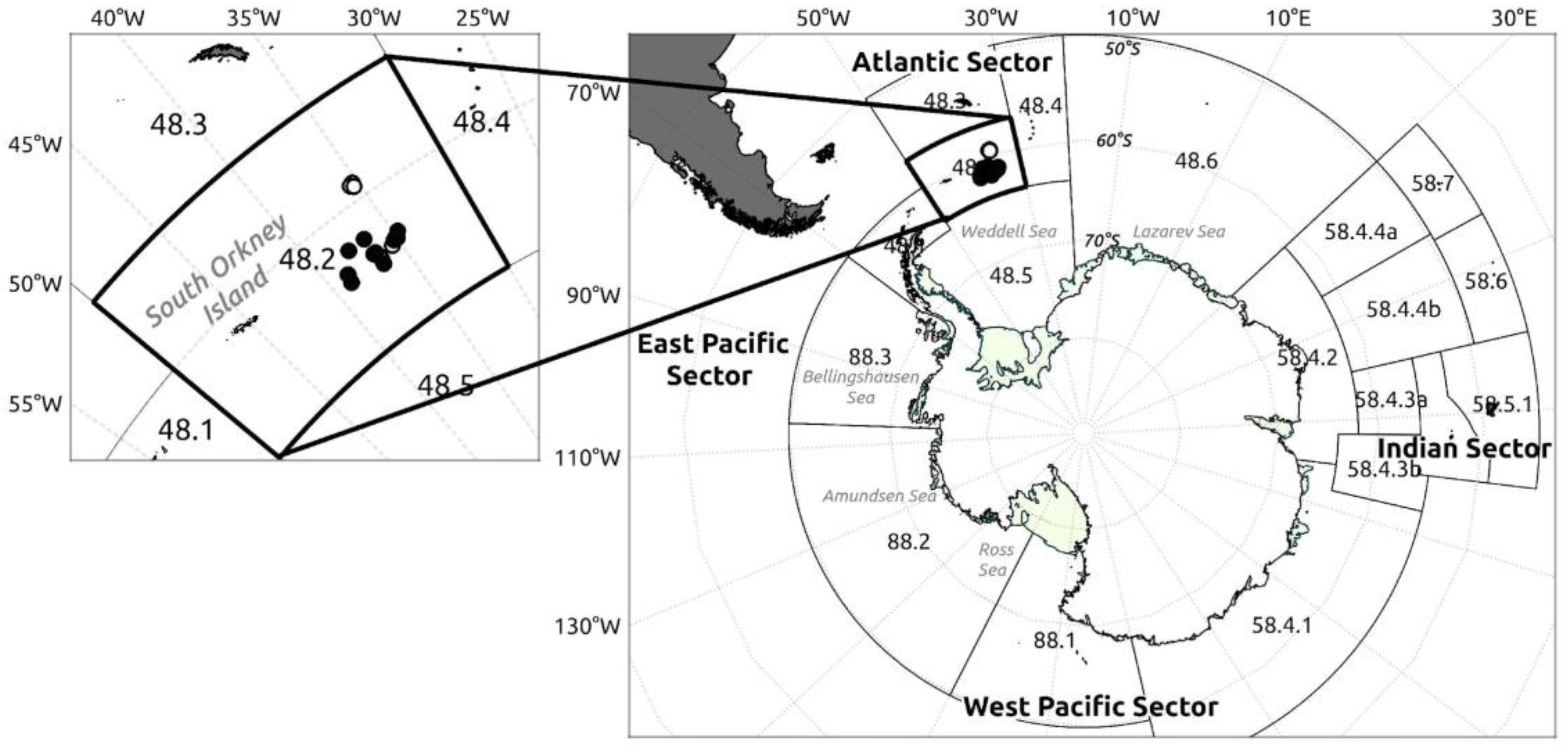
Figure 2.
Transverse section of a sagittal otolith from an adult Dissostichus mawsoni specimen (>135 cm TL), polished and analysed by LA-ICPMS. A) A total of 17 ablations (diameter = 65 μm) are observed along the primordial-ventral margin axis of the otolith. The first six ablations represent the juvenile stage, while the last three correspond to the adult stage. B) Micro-drill trajectory programmed to extract nuclear (red polygon) and marginal (yellow polygon) regions of the sagittal otolith for isotopic composition analysis.
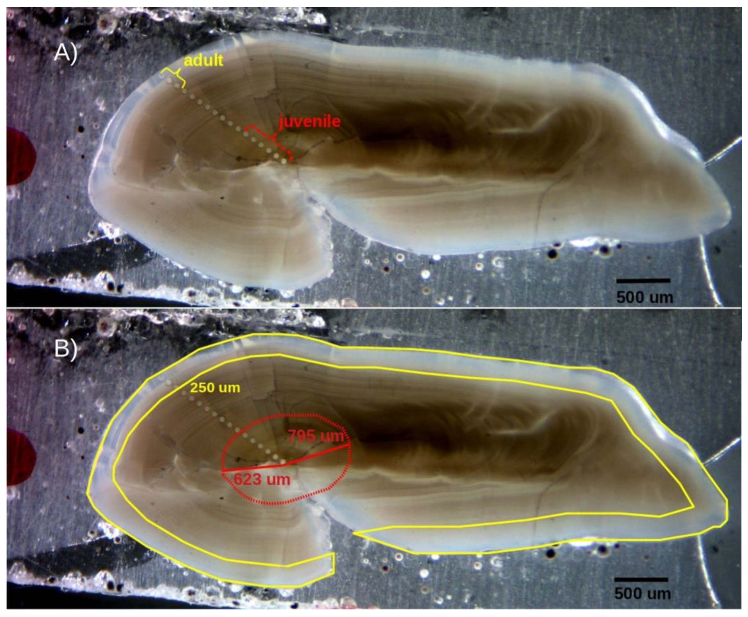
Figure 3.
Schematic representation of the geolocation method used to identify nursery areas of Dissostichus mawsoni in this study. A-B) Interpolated values of temperature and salinity in the water column, used as covariates for (C) kriging δ18O. D) Probability distribution functions for expected δ18O values at each location and layer. E) Observed δ18O values in sections of sagittal otoliths of D. mawsoni. F) Synoptic maps of averaged individual probabilities of occurrence within each grid cell.
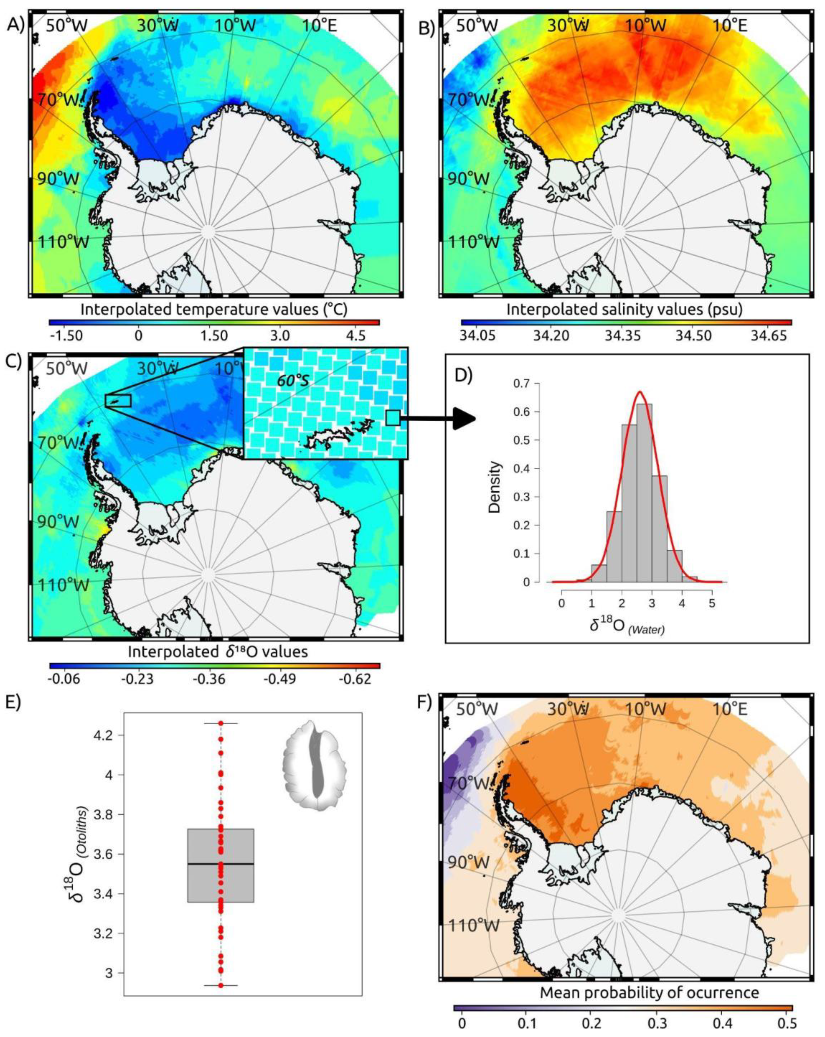
Figure 4.
Elemental compositions (Li, Mg, Mn, Sn, Na, Cr, Sr, and Ba relative to Ca) and isotopic signatures (δ18O and δ13C) of nuclear and marginal otolith regions, representing the first year of life and the adult life stages of Antarctic toothfish (Dissostichus mawsoni) adults from the South Orkney Islands. Boxes represent the 25th and 75th percentiles, with whiskers extending up to 1.5 times the interquartile range or the most distant observation within this range. Different superscript letters indicate significant differences (p < 0.05) under the null hypothesis of no difference between means.
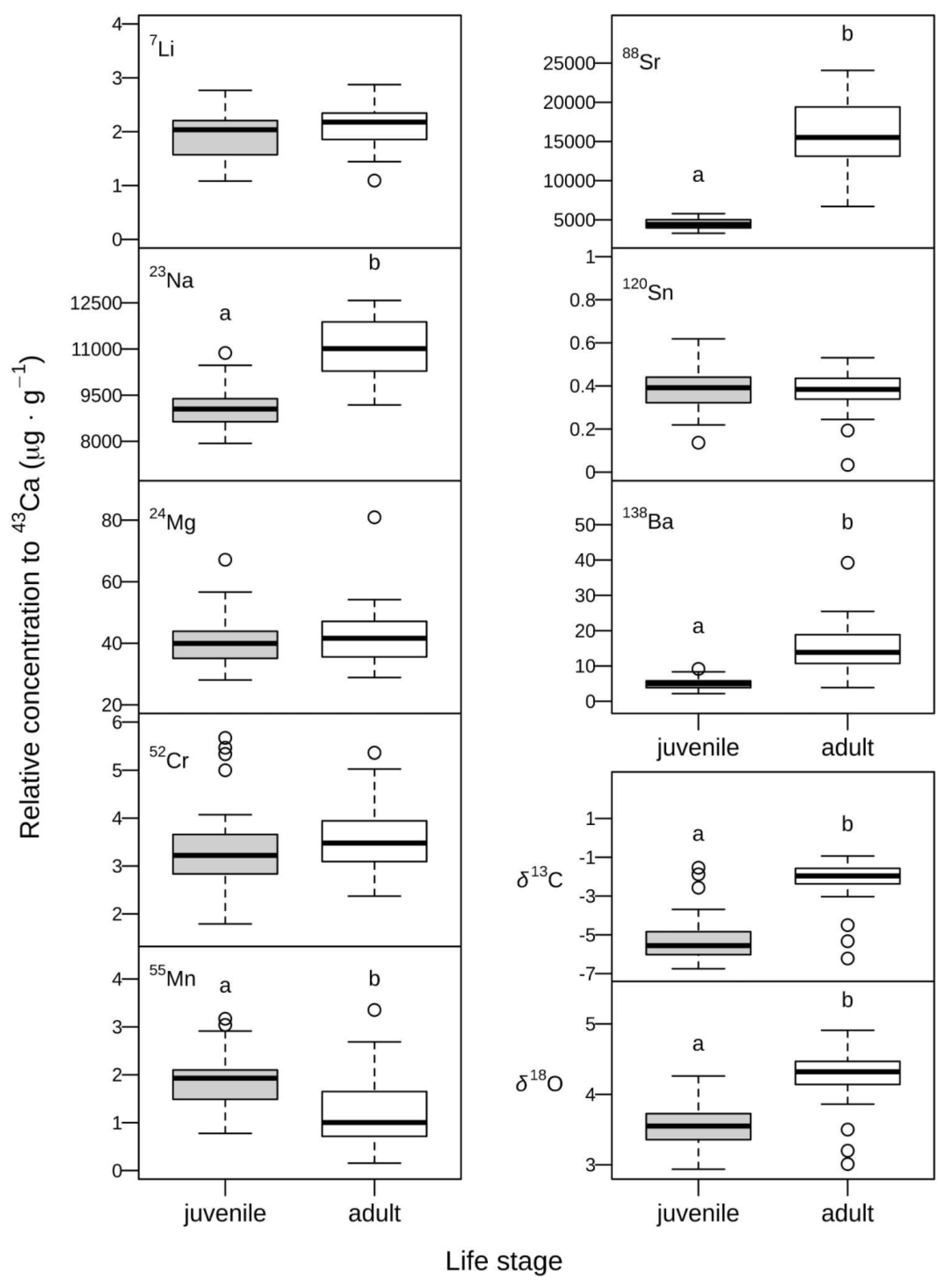
Figure 5.
Chemical signatures observed in the nuclear and marginal regions of otoliths, representing the juvenile and adult stages of Antarctic toothfish (Dissostichus mawsoni) from the South Orkney Islands. (A) Elemental composition (Na, Mg, Mn, Sr, and Ba relative to Ca) visualized using Non-Metric Multidimensional Scaling (NMDS). (B) Isotopic composition of δ13C and δ18O.
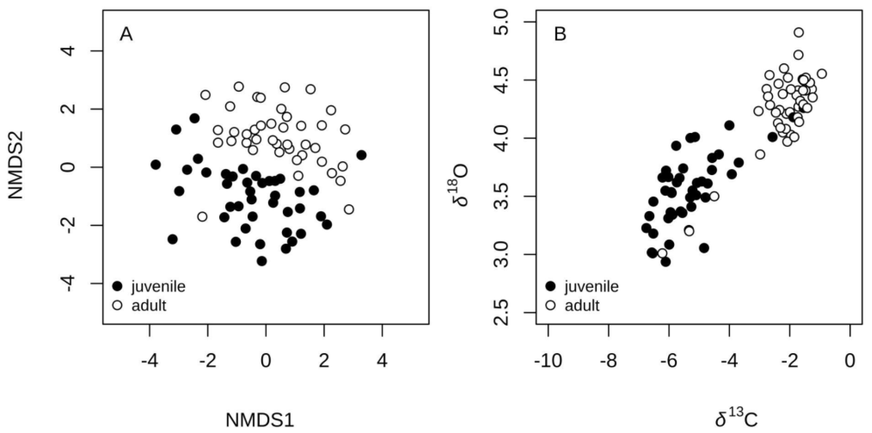
Figure 6.
Strontium and barium profiles (relative to Ca) along the core-to-dorsal edge transect of otolith sections from Antarctic toothfish (Dissostichus mawsoni). The shaded area represents the estimated age range (ablations) where 50% of otoliths (P25–P75) showed the highest probability of detecting a change in element concentrations between ablations. The vertical dashed line indicates the mean age at which otoliths displayed the highest probability, based on the Bayesian change-point analysis described by Barry and Hartigan (1993).
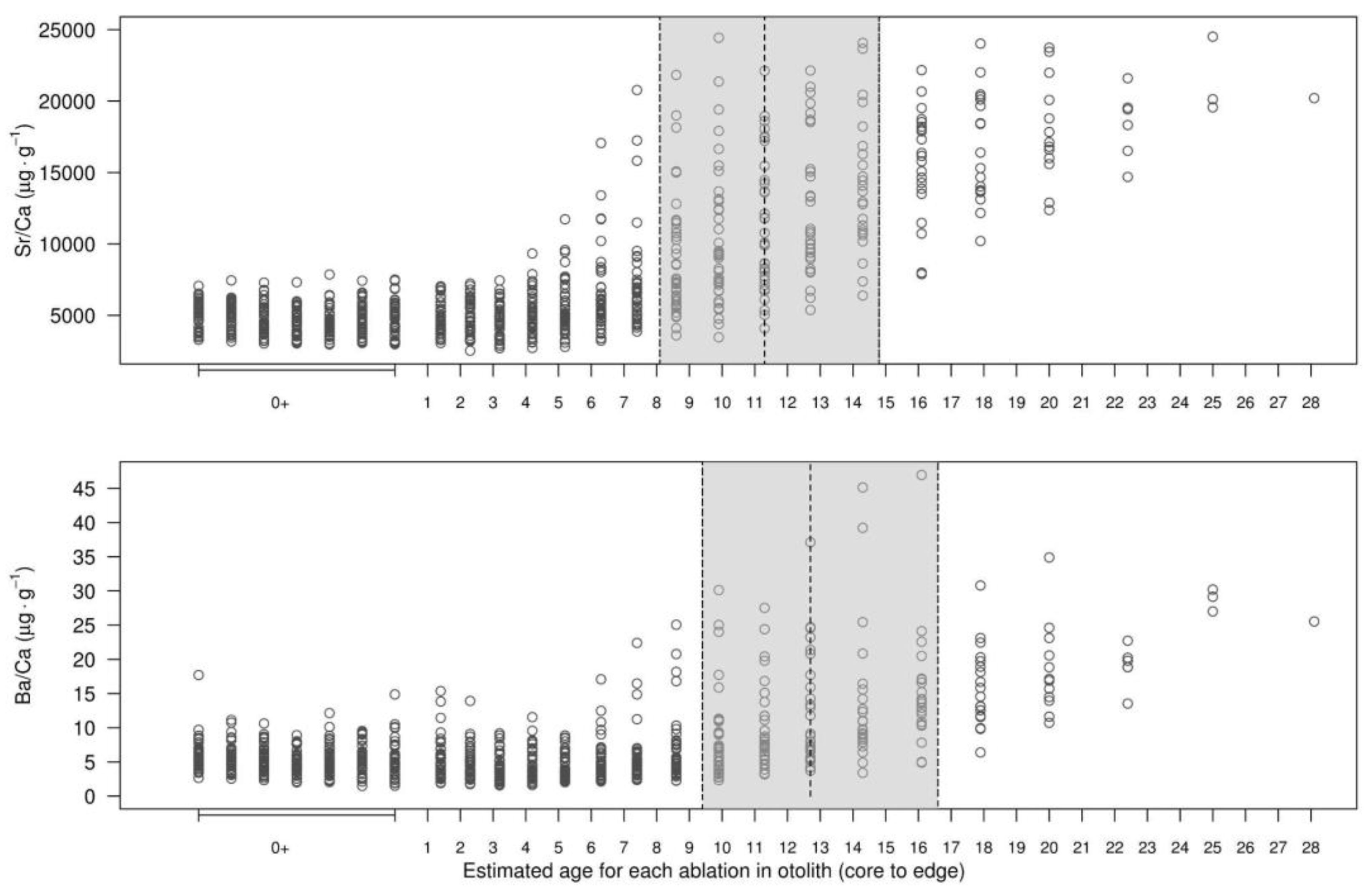
Figure 7.
Mean probability of occurrence of Antarctic toothfish Dissostichus mawsoni as young-of-the-years by location and depth stratum. Computed by comparing observed values of δ18O in nuclear otolith regions of adult fish to probability distribution functions estimated from seawater δ18O by location and depth stratum.
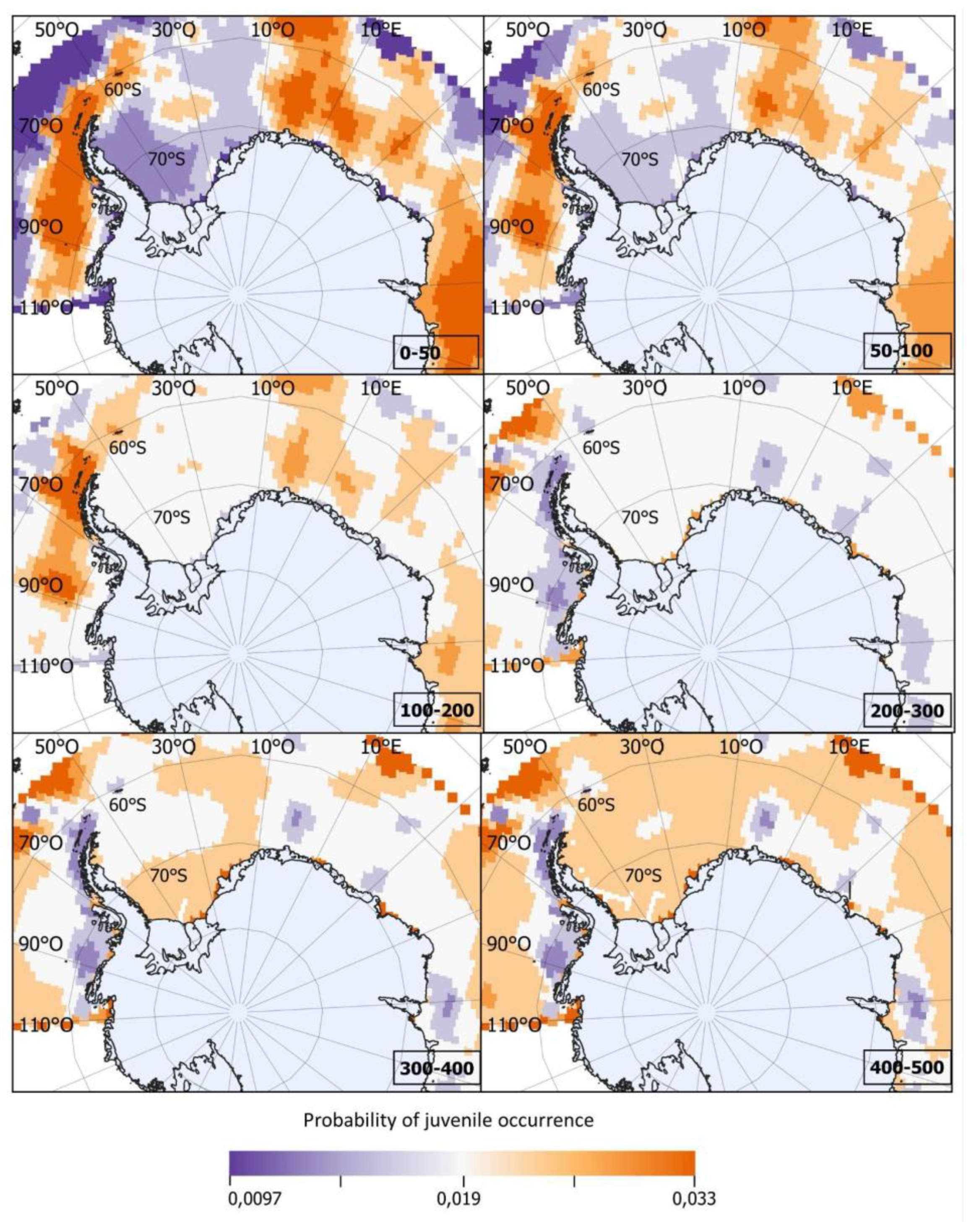
Figure 8.
Schematic representation of areas with the highest probabilities (95th percentile) of origin for Dissostichus mawsoni adults from Source 1 (green) and Source 2 (blue), based on the most informative finite mixture distribution model (FMD). The analysis used elemental composition (Li, Mg, Mn, Sn, Na, Cr, Sr, Ba) and stable isotopes (δ¹⁸O, δ¹³C) in otoliths from cohorts (1989–2002) sampled around the South Orkney Islands in 2016 and 2018. Dashed lines indicate stock hypotheses (Söffker et al., 2018): A = Weddell Sea population, A1 = Weddell subpopulation 1, A2 = Weddell subpopulation 2, B = Indian Ocean population, C = Bellingshausen population.


Table 1.
Estimated means and standard deviations for relative concentrations of selected elements (μmol·μmol Ca⁻¹) and stable isotopes (δ¹⁸O and δ¹³C) in nuclear and marginal regions representing juvenile (YOY) and adult life stages of the Antarctic toothfish (Dissosticus mawsoni). Paired differences between stages were computed within individuals (n = 42 and 45 for elemental and isotopic signatures, respectively), fitted through a univariate linear mixed model, and tested (H₀: intercept = 0) using a t-test.
| Elemental concentrations (μmol·μmol Ca-1) and stable isotopic ratios (‰) | Life stage | Paired t-test results | |||||
| Juvenile | Adult | ||||||
| Mean | SD | Mean | SD | t | df | pr>t | |
| Li | 1.9 | 0.4 | 2.1 | 0.4 | -3.21 | 25 | <0.01 |
| Na | 9057.3 | 675.1 | 11026.6 | 928.8 | -11.18 | 25 | <0.001 |
| Mg | 42.6 | 15.5 | 43.9 | 13.8 | -0.64 | 23 | 0.53 |
| Cr | 3.3 | 0.87 | 3.8 | 1.1 | -3.86 | 23 | <0.001 |
| Mn | 1.9 | 0.54 | 1.19 | 0.710 | 5.30 | 23 | <0.001 |
| Sr | 4461.9 | 680.9 | 15683.1 | 4385.2 | -21.32 | 23 | <0.001 |
| Sn | 0.4 | 0.1 | 0.4 | 0.1 | 0.71 | 23 | 0.48 |
| Ba | 4.9 | 1.5 | 15.0 | 7.2 | -8.74 | 23 | <0.001 |
| δ18O | 3.6 | 0.3 | 4.3 | 0.3 | -7.50 | 28 | <0.001 |
| δ13C | -5.3 | 1.1 | -2.2 | 1.0 | -10.49 | 28 | <0.001 |
Table 2.
Bayesian Information Criteria (BIC) for the three best-fitting unsupervised mixture models applied to elemental and isotopic signatures observed in the nuclear regions of otoliths from Dissostichus mawsoni adults, representing cohorts from 1989 to 2002 and sampled around the South Orkney Islands in 2016 and 2018.
| Number of sources in the mixture | Elemental signatures | Isotopic signatures | ||
| BIC | ΔBIC | BIC | ΔBIC | |
| 1 | -755.0 | 15.3 | -208.5 | 8.1 |
| 2 | -740.3 | 0 | -200.4 | 0 |
| 3 | -751.1 | 11.2 | -208.3 | 7.9 |
Table 3.
Nursery-source contributions and their corresponding chemical signatures in the nuclear regions of otoliths, estimated for Dissostichus mawsoni adults from cohorts spanning 1989 to 2002 and sampled around the South Orkney Islands in 2016 and 2018.
Table 3.
Nursery-source contributions and their corresponding chemical signatures in the nuclear regions of otoliths, estimated for Dissostichus mawsoni adults from cohorts spanning 1989 to 2002 and sampled around the South Orkney Islands in 2016 and 2018.
| Mean ± SE | ||
| Source 1 | Source 2 | |
| Proportional contribution | ||
| Elemental signatures (n=37) | 0.74 ± 0.061 | 0.26 ± 0.061 |
| Stable isotope signatures (n=39) | 0.92 ± 0.035 | 0.08 ± 0.035 |
| Elemental signature | ||
| Li:Ca | 1.66 ± 0.071 | 2.33 ± 0.047 |
| Na:Ca | 8912 ± 175 | 8926 ± 105 |
| Mg:Ca | 44.59 ± 3.523 | 42.64 ± 1.191 |
| Cr:Ca | 3.41 ± 0.185 | 2.98 ± 0.084 |
| Mn:Ca | 1.5 ± 0.093 | 1.98 ± 0.087 |
| Sr:Ca | 5241 ± 125 | 4469 ± 124 |
| Sn:Ca | 0.44 ± 0.019 | 0.34 ± 0.013 |
| Ba:Ca | 6.01 ± 0.262 | 4.08 ± 0.205 |
| Isotopic signature | ||
| δ18O | 3.51 ± 0.050 | 4.15 ± 0.013 |
| δ13C | -5.51 ± 0.130 | -2.00 ± 0.052 |
Disclaimer/Publisher’s Note: The statements, opinions and data contained in all publications are solely those of the individual author(s) and contributor(s) and not of MDPI and/or the editor(s). MDPI and/or the editor(s) disclaim responsibility for any injury to people or property resulting from any ideas, methods, instructions or products referred to in the content. |
© 2024 by the authors. Licensee MDPI, Basel, Switzerland. This article is an open access article distributed under the terms and conditions of the Creative Commons Attribution (CC BY) license (http://creativecommons.org/licenses/by/4.0/).
Copyright: This open access article is published under a Creative Commons CC BY 4.0 license, which permit the free download, distribution, and reuse, provided that the author and preprint are cited in any reuse.


