
Submitted:
26 November 2024
Posted:
26 November 2024
You are already at the latest version
Abstract
The use of High-Strength LowAlloy (HSLA) steels for welded parts and structural assemblies is increasingly common. Steel S700MC is one of the most widely used HSLA steels, especially in the automotive and manufacturing industries. It combines high-strength properties with good ductility, toughness and reasonable technological workability in forming and welding. Despite all these advantages, there is still not enough information describing the processes and changes in material properties that occur in different heating and cooling conditions. The present study aims to describe such processes in detail using dilatometric studies. Thus, it results not only in a newly developed Continuous Cooling Transformation (CCT) diagram of the S700MC steel, but also in an assessment of the heating rate effect on the change of austenitizing temperatures. Then, the influence of the cooling rate on the bandwidth of transformation changes is defined, and the impact of temperature cycles on the changes in mean grain size is assessed. A comprehensive study of this type has not yet been published for S700MC steel.
Keywords:
HSLA Steel
; S700MC
; CCT Diagram
; Dilatometry Analysis
; Phase Transformations
1. Introduction
Welded structures comprise a significant part of industrial production, either as final products or as partial components. In doing so, there is a constant emphasis on production efficiency and sufficient strength properties with the lowest possible weight and adequate durability in various environmental conditions [1,2,3]. The trend is, therefore, to use higher-strength steels, usually with yield strength values exceeding 460 MPa. At the same time, demands are placed on the corresponding toughness and technological workability of such materials. These requirements are met in particular by HSLA steels, which combine high strength with good resistance to brittle failure [4,5], even at negative temperatures [6,7]. The great advantage of HSLA steels is their excellent cold formability and relatively good weldability due to their strictly controlled chemical composition, especially for microalloying elements. The microalloying elements mainly include V, Ti, and Nb, which form carbides, nitrides, and carbonitrides at grain boundaries. These subsequently contribute to matrix strengthening and grain refinement [8,9,10,11]. HSLA fine grain steels with yield strengths up to 700 MPa are thus strengthened mainly by grain boundaries, strain hardening and precipitation. For steels with higher yield strengths, another strengthening mechanism is added, which is phase transformation leading to martensite or bainite [12,13,14].
HSLA steels have a wide range of applications across the manufacturing spectrum. They are used in automotive, crane manufacturing, bridge construction, oil and gas platform construction. These steels are widely used to manufacture statically and dynamically loaded components, wind generator supports, or high-pressure vessels [15,16,17,18,19,20]. As already indicated, the weldability of fine-grained steels is good, mainly due to the low carbon content and the limited content of alloying elements. Compared to welding of conventional structural steels, it is recommended to limit the heat input per unit length of weld to 10 kJ·cm-1 when welding fine grain steels, mainly because of the intense grain coarsening in the highly heated Heat Affected Zone (HAZ) [21], and for high-strength steels also because of the softening zone [22,23].
Different fusion welding methods with varying shapes of temperature cycles and various values of the t8/5 parameter can be used for welding HSLA steels. The most commonly used method is MAG. In addition, laser and hybrid methods can also be used, as well as (to a limited extent) the TIG method. Studies of the effect of fusion welding by MAG on the weld structure of S700MC steel have been carried out, e.g., in [24,25] or for the hybrid form of welding [26]. Numerical simulations [27] are an integral part of understanding the processes involved in welding HSLA steels, specifically S700MC steel, concerning microstructure, mechanical properties, grain coarsening, etc. In all of the above cases, for the planning and realization of welding experiments, it is advisable, and in the case of simulations, almost essential, to have a complete CCT diagram, which unfortunately could not be traced in the available sources.
Therefore, the study presented here aimed to determine the missing information related to the processes that occur under different heating and cooling conditions. Based on comprehensive dilatometric tests, it is not only possible to cover the complete transformation changes over a wide range of cooling rates (0.03 to 250 °C·sec-1) but also, in agreement with other findings, to assess the influence of heating rate on the shift of Ac1 and Ac3 transformation temperatures [28,29], or the effect of specific temperature cycles on grain coarsening [29].
2. Materials and Methods
2.1. Experimental Material
In this work, fine grain steel designated S700MC according to ISO 10027-1 and 1.8974 according to ISO 10027-2, belonging to the HSLA (High Strength Low Alloy) steel group, was used for the experimental work. It means to the group of microalloyed thermomechanically rolled steels. It is one of the most widely used HSLA steels [13,30,31]. Due to its minimum guaranteed yield strength of 700 MPa, its strictly controlled chemical composition and, above all, its thermomechanical processing, it exhibits high strength, good cold formability and good weldability [25,32]. It is microalloyed mainly with elements such as Al, Ti, Nb and V, which (together with carbon and nitrogen) form fine carbides, nitrides or carbonitrides, reducing the susceptibility to grain growth [5]. All this has an influence on the excellent mechanical properties, especially the brittle properties, even at lower temperatures.
The steel was supplied in the form of a 12 mm thick plate. The chemical composition of S700MC steel was measured using a Bruker Q4 TASMAN spectrometer (Bruker Corporation, Billerica, Massachusetts, USA). The measurements were performed on the test specimens at four differently oriented locations. Table 1 shows the mean value of the four measurements and gives the chemical composition values defined by EN 10149-2.
The mechanical properties of the supplied S700MC material, such as Proof Yield Strength (PYS - Rp0.2), Ultimate Tensile Strength (UTS - Rm), Uniform Ductility (Ag) and Total Ductility (A40mm), were measured at room temperature (RT) on a test device TIRA Test 2300 (Tira GmbH, Schalkau, Germany). The measurements were performed on five samples according to EN ISO 6892-1 standards. The mean values of the measured material properties, including standard deviations, are given in Table 2.
S700MC is a low alloy steel, exhibiting a ferritic-bainitic structure in its initial state. The microstructure of the tested material was evaluated by light microscopy. A Scanning Electron Microscope (SEM) TESCAN Mira 3 (Tescan Orsay Holding, a.s., Kohoutovice, Czech Republic) with an EBSD detector (Electron Back Scatter Diffraction) was used to determine the mean grain size. The following parameters were used for the analysis: accelerating voltage HV = 20 kV, measuring step size 0.2 μm, measured area 500 x 500 μm2. The resulting value of the mean grain size of the S700MC material in the initial state was 4.29 μm. The structure and analysis of the mean grain size is shown in Figure 1.
2.2. Samples Preparation
Dilatometric tests were carried out as a basis for creating a CCT diagram and then to assess the influence of the heating rate on the shift in transformation temperatures and the impact of temperature cycles on the change in mean grain size. All experiments were carried out on a DIL 805L quenching dilatometer (TA Instruments, New Castle, Delaware, USA), which allows to measure the change of sample length to an accuracy of 0.01 μm. An induction coil provides sample heating with feedback using an R-type thermocouple, which is capacitor welded to the test sample. Although the device declares a sample heating capability of 1000 °C·sec-1, the usable dilatometric curves are for maximum heating rates of 250 °C·sec-1 [28].
For the dilatometric analysis, circular specimens with a diameter of 4 mm and a length of 10 mm were fabricated, as seen in Figure 2. The faces of the specimens must be parallel, and the maximum surface roughness should be within 3.2 μm.
2.3. Determination of the Dilatometric Curve
To construct the CCT diagram of S700MC steel, 16 different temperature cycles were applied to the samples in the quenching dilatometer. Six of them with heating rates ranging from 0.1 to 250 °C·sec-1 were used to determine the effect of the heating rate on the shift of transformation temperatures. The selected parameters of these temperature cycles are shown in Table 3. The remaining eleven temperature cycles with different cooling rates ranging from 0.03 to 200 °C·sec-1 were used to generate the CCT diagram. Their selected parameters are shown in Table 4. The sample with a heating and cooling rate of 10 °C·sec-1 was same for both experiments. The temperature delay at austenitizing temperature was 30 seconds in all cases. A graphical representation of the temperature cycles for the heating and cooling phases is shown in Figure 3.
The last part of the dilatometric tests was devoted to assessing the effect of heating and cooling rates on the intensity of grain coarsening, i.e. on the change in mean grain size. For this part of the experiments, temperature cycles with different rates in the heating and cooling part were used. Specifically, combinations of heating rates ranging from 0.1 to 10 °C·sec-1 and cooling rates ranging from 0.03 to 200 °C·sec-1 were used. The parameters of these specific temperature cycles are shown in Table 5.
2.4. Methodology for Evaluation Dilatometry Curves
A correct evaluation of the dilatometric curves is essential to obtain information about the start and end of the transformation changes and to consider any shift in the transformation temperatures. There are several ways of determining the transformation temperatures. However, the three tangents and the first derivative method are the most commonly used. Relevant results can be obtained from both evaluation methods. In some cases, these two methods are combined and the resulting transformation temperature value is given by the mean of these methods.
The basis of the three tangents method for the standard transformation is shown schematically in Figure 4. Specifically, in this case, the evaluation of the heating part of the dilatometric curve of the sample labelled as H1_C10 is used to obtain the transformation temperatures Ac1 = 811 °C and Ac3 = 859 °C. In the case of multiple transformations, more tangents are then used, but the method of determining the specific transformation temperature remains identical.
The second way of evaluating transformation temperatures is the first derivative method. The dependence of the length change rate on temperature is obtained by deriving the obtained dilatometric curve, i.e., the dependence of the length change rate on temperature. The temperature at which the change in length rate is zero is the temperature of the beginning or end of the phase transformation accompanied by volume changes. Figure 5 shows the basis of the first derivative method, also in this case for the sample labelled as H1_C10. The transformation temperatures were evaluated as Ac1 = 807 °C and for Ac3 = 861 °C. The same procedure is followed to assess the cooling part of the curves.
2.5. Evaluation of Microstructure
Once the beginnings and ends of the phase transformations for a given heating and cooling rate have been determined, a metallographic evaluation of the samples must be performed. This was done on each of the dilatometric samples. The specimen was always cut in half on a cut-off machine for metallographic sample preparation with a cooled diamond wheel of wide 1 mm. Both halves were subsequently used at the point of cut - one for microstructure evaluation and hardness measurement, the other for SEM and EBSD analysis. Samples for microstructural analysis were standardly ground and then polished by diamond suspension with grain sizes of 3 and 1 um. Samples for SEM and structural analysis were finally polished with OP-S suspension containing oxides with a grain size of 0.25 um. The evaluation was performed on a TESCAN Mira 3 electron microscope.
After the microstructure was done, the samples were used for hardness measurements using the Vickers method (HV). An automatic hardness tester Qness Q30A (ATM Qness GmbH, Mammelzen, Germany) was used for hardness measurement and the measurement was performed with a load of 98.07 N (HV10). Nine impressions were performed on each specimen, from which the mean value and standard deviation were determined.
3. Results and Discussion
3.1. Effect of the Heating Rate on Shifts in the Transformation Temperatures Ac1 and Ac3
For the evaluation of dilatometric curves, either in the heating region for the determination of the Ac1 and Ac3 transformation temperature shift or in the cooling phase of the assessment of the phase transformations, both methods presented in Section 2.4, i.e. the three tangent method and the first derivative method, were used. For different combinations of heating rates (according to Table 3), the start and end temperatures of austenite transformation were determined using both methods.
Regarding the evaluation by both methods, the maximum difference in determining the transformation temperatures was 1.7 % (14 °C deviation) for the temperature cycle with the designation H5_C0.3. The obtained deviations depend on the correct application of the methods and, therefore, on accurately evaluating the transformation temperatures. Table 6 gives the values of the transformation temperatures obtained for both methods for all used temperature cycles. Figure 6 graphically shows the influence of heating rate on the shift of the transformation temperatures, including the trend line.
From the trends of the curves shown in Figure 8, it is clear that the values of the transformation temperatures of the beginning and end of austenitization of Ac1 and Ac3 increase together with increasing heating rate. The trend of transformation temperature of Ac1 is linear with 99.1 % accuracy. In contrast, the Ac3 temperature only agrees with the linear trend of 69.2 %. In fact, from heating rates above 10 °C·sec-1, the trend for Ac3 increases more sharply than for lower rates. At the same time, it is clear that the region between Ac1 and Ac3 decreased slightly (from 0.1 to 100 °C·sec-1) as the heating rate increased. The change in austenitization bandwidth as a function of the heating rate is shown in Figure 7, including the trend line.
For the CCT diagram, the values of the start and end transformation temperatures were determined as the average value evaluated by the two methods used at the slowest heating rate of 0.1 °C·sec-1. Specifically, these values were as follows: Ac1 = 794 °C and Ac3 = 860 °C.
3.2. Transformation Changes in the Cooling Phase
A total of nine different cooling rates, uniformly spaced in log coordinates from 0.03 to 200 °C·sec-1, were used to describe the transformation processes during cooling. The results are shown in Table 7. Again, both methods (three tangents method and first derivative method) were used to determine the transformation temperatures of austenite decomposition into the individual phases. At constructing the CCT diagram of S700MC steel, it was found necessary to specify the origin of the transformation regions in the range of cooling rates from 30 to 200 °C·sec-1. Therefore, two dilatometric experiments were additionally completed with cooling rates of 55 °C·sec-1 and 142 °C·sec-1. For most of the cooling rates, a multiphase transformation occurred.
The whole transformation process, from heating to cooling, can generally be divided into several stages. Austenitization occurs when steels are heated above the transformation temperature Ac1. Austenite grains are formed at the expense of the original phases, and the growth of these austenitic grains occurs when they are kept at a high temperature above the transformation temperature [5,33]. This generally has an effect on the change in mechanical and brittle properties [34,35]. When steels cool below the transformation temperature, phase transformations take place, which are manifested by a change in the crystal structure. Depending on the cooling rate, the phase transformation can take place in two ways, namely diffusion or non-diffusion transformation [36]. This results in different structures and different grain sizes.
As can be seen from Figure 8, the cooling rate in S700MC steel affects the width of the temperature interval in which the structural transformation occurs. At slow cooling rates from 0.03 to 1 °C·sec-1, the width of the transformation band is approximately 30 °C, respectively 50 °C (depending on the used evaluation method) and corresponds to the diffusive transformation of austenite to ferrite and pearlite. As the cooling rate increases, the width of the transformation region expands until it is more than double. In the interval of cooling rates from 3 to 100 °C·sec-1, the width of the transformation zone varies from approximately 80 °C to 140 °C, again depending on the evaluation method used. Both diffusive and non-diffusive processes occur in this interval. At a cooling rate of 3 °C·sec-1, a ferritic-bainitic structure is obtained. By further increasing the cooling rate, martensite is gradually added to ferrite and bainite up to a cooling rate of 30 °C·sec-1. Above this rate, up to 100 °C·sec-1, only a bainitic-martensitic structure is obtained. In this interval, the width of the transformation region is greatest. Above a cooling rate of 100 °C·sec-1, only the diffusion-free transformation region of austenite to low-carbon martensite is present. Here, the transformation region narrows considerably. The trends described above are also evident from the trend lines in Figure 8 for both evaluation methods of the transformation temperatures.
3.3. Hardness Evaluation on the Dilatometry Samples
As already partially mentioned in Section 2.5, the hardness of HV10 was measured on each specimen that was subjected to the temperature cycle on the dilatometer. All measured values, including the standard deviation, are shown in Table 8. The hardness was also measured on the S700MC material in the initial state, and a value of 272 ± 1.6 HV10 was found. According to the other measured values, this corresponds to a cooling rate of approximately 64 °C·sec-1. The effect of the cooling rate on the hardness values can be seen in Figure 9.
3.4. Design of CCT Diagram
To create a CCT diagram, in addition to determining the transformation temperatures, it is necessary to know what final structures have been achieved for a given cooling rate. Figure 10 shows the microstructure for the base material and for samples obtained with cooling rates from 0.03 to 200 °C·sec-1. By evaluating the microstructure of each sample, it was found that in the interval of cooling rates from 0.03 to 1 °C·sec-1, the microstructure contains a mixture of ferrite and bainite with a gradual increase in martensite. A further increase in cooling rate results in a bainitic-martensitic structure, and above a cooling rate of 100 °C·sec-1, only a martensitic structure is achieved.
The resulting CCT diagram of S700MC steel is shown in Figure 11. This diagram corresponds to the chemical composition in Table 1 and the mechanical properties in Table 2. A change in chemical composition may affect the final form of the diagram. However, due to the relatively strictly monitored chemical composition of HSLA steels, such changes will only be negligible.
3.5. The Effect of Applied Temperature Cycles on the Changes of Mean Grain Size
An assessment of the effect of the applied thermal cycle on the mean grain size, performed with an EBSD (Electron Backscatter Diffraction) detector, for all cooling rates is shown in Figure 12. The measured mean grain sizes after EBSD analysis for the equivalent circle diameter (ECD) are shown in Table 9. From the values shown in Table 9, a graph (Figure 13) was constructed to show the trend of the change in mean grain size as a function of the applied cooling rate. The graph shows that the grain coarsening is negligible for samples heated at 10 °C·sec-1 to 1100 °C with a temperature delay time of 30 sec and cooling rates of 10 °C·sec-1 or more. The grain refinement at a cooling rate of 200 °C·sec-1 is interesting. Here, it would be reasonable to expect the same grain size as for the base material since the sample is not plastically deformed during the dilatometer cycle, and the conditions for intensive formation of new grain nuclei are not created. However, it is clear from the mean grain sizes and standard deviations given in Table 9 that the result is within the tolerance range of the grain size of the base material.
4. Conclusions
The study presented in this paper aimed to show in detail the processes and material changes that occur in S700MC steel when temperature cycles with different heating and cooling rates are applied. The findings are based on the dilatometric experiments complemented by structural analyses, hardness measurements and evaluation of the change in mean grain size. Thus, the dependences of the transformation temperature shift and the width of the transformation bands based on the heating and cooling rates were obtained, as well as a complete CCT diagram of the S700MC steel. A comprehensive study of this type has not yet been published for S700MC steel. The main conclusions of the above research are as follows:
- The study has shown that both evaluation methods, i.e. the three tangents method and first derivation method, can be used with sufficient accuracy to determine the transformation temperatures in the heating phase. The maximum deviation between the two methods was 1.7 %. Interestingly, the more significant deviations were at the beginning of the transformation for the Ac1 temperature. For the Ac3 temperature, the maximum deviation was less than 0.9 %.
- Increasing the heating rate has a negligible effect on the bandwidth of the austenitic transformation, as seen from the trend lines in Figure 6.
- For the CCT diagram, the values of the start and end transformation temperatures were determined as the average of the temperatures evaluated by the two methods used at the slowest heating rate of 0.1 °C·sec-1. Specifically, these temperatures were Ac1 = 794 °C and Ac3 = 860 °C, resp.
- The evaluation of the transformation changes during cooling already showed significant differences between the different methods used. For cooling rates in the interval 0.03 to 30 °C·sec-1, the maximum deviation was 3.41 %, which is still acceptable. However, a further increase in cooling rate to 100 °C·sec-1 increased the deviation to almost 5 % and even to nearly 8 % for 200 °C·sec-1. For high cooling rates, more relevant results were obtained with the three tangents method.
- In contrast, the effect of the cooling rate on the bandwidth of the transformation temperatures is significant compared to the heating rate. For slow cooling rates in the interval 0.03 to 1 °C·sec-1, the transformation bandwidth is constant (ferritic-perlitic transformation). Thereafter, the transformation temperature bandwidth more than doubles up to a cooling rate of 100 °C·sec-1. Above this rate, only the non-diffusion martensitic transformation is present in S700MC steel, and the transformation bandwidth returns to the value corresponding to the slow cooling rates.
- The hardness measurements of the samples showed a steady increase in hardness with the increasing percentage of phases containing carbon in the form of carbides or supersaturated solid solution. The dependence was tested using a linear regression model with a logarithmic function. The correlation coefficient R2 was higher than 0.98, approximating the measured hardness values at a given cooling rate with the regression line. The hardness value HV10 increased from 140 HV10 to 324 HV10 over the cooling rate range of 0.03 to 200 °C·sec-1. The hardness of the base material 272 HV10 thus corresponds to cooling rates of 64 °C·sec-1.
- The generated CCT diagram (Figure 11) correlates with the chemical composition in Table 1. A change in the chemical composition may affect the final form of the diagram. However, given the relatively strictly monitored chemical composition of HSLA steels, it can be assumed that such changes will only be elementary.
Author Contributions
Conceptualization, J.M. and D.K.; methodology J.M. and D.K.; validation, J.M. and M.Š.; formal analysis, D.K.; investigation, D.K. and J.M.; resources, J.M. and D.K.; data curation, D.K., J.M. and M.Š.; writing—original draft preparation, D.K.; writing—review and editing, J.M.; visualization, D.K.; supervision, J.M.; project administration, D.K.; funding acquisition, D.K.
Funding
This research was funded by the Student Grant Competition of the Technical University of Liberec, grant number SGS-2024-5435, “Assessment of the effect of welding on grain growth kinetics and fatigue life of fine-grained steels joints“.
Institutional Review Board Statement
Not applicable.
Informed Consent Statement
Not applicable.
Data Availability Statement
Not applicable.
Conflicts of Interest
The authors declare no conflict of interest.
References
- Chmielewski, T.; Golański, D. The Role of Welding in the Remanufacturing Process. Welding International 2015, 29, 1–4. [Google Scholar] [CrossRef]
- Shipitsyn, S.Ya.; Babaskin, Yu.Z.; Kirchu, I.F.; Smolyakova, L.G.; Zolotar, N.Ya. Microalloyed Steel for Railroad Wheels. Steel Transl. 2008, 38, 782–785. [Google Scholar] [CrossRef]
- Meester, B. The Weldability of Modern Structural TMCP Steels. ISIJ International 1997, 37, 537–551. [Google Scholar] [CrossRef]
- Illescas, S.; Fernández, J.; Asensio-Lozano, J.; Sanchez-Soto, M.; Guilemany, J.M. Study of the Mechanical Properties of Low Carbon Content HSLA Steels. Revista de Metalurgia 2009, 45. [Google Scholar] [CrossRef]
- Moravec, J.; Novakova, I.; Sobotka, J.; Neumann, H. Determination of Grain Growth Kinetics and Assessment of Welding Effect on Properties of S700MC Steel in the HAZ of Welded Joints. Metals 2019, 9, 707. [Google Scholar] [CrossRef]
- Sastry, C.; Hariharan, P.; M, P. kumar; Manickam, M.A. Experimental Investigation on Boring of HSLA ASTM A36 Steel under Dry, Wet, and Cryogenic Environments. Materials and Manufacturing Processes 2019, 34, 1–28. [Google Scholar] [CrossRef]
- Pamnani, R.; Jayakumar, T.; Vasudevan, M.; Sakthivel, T. Investigations on the Impact Toughness of HSLA Steel Arc Welded Joints. Journal of Manufacturing Processes 2016, 21, 75–86. [Google Scholar] [CrossRef]
- Fernández, J.; Illescas, S.; Guilemany, J.M. Effect of Microalloying Elements on the Austenitic Grain Growth in a Low Carbon HSLA Steel. Materials Letters - MATER LETT 2007, 61, 2389–2392. [Google Scholar] [CrossRef]
- Barbaro, F.; Zhu, Z.; Kuzmikova, L.; Li, H.; Jian, H. Weld HAZ Properties in Modern High Strength Niobium Pipeline Steels. In; 2015; pp. 453–457.
- Rakshe, B.; Patel, J. Modern High Strength Nb-Bearing Structural Steels. 2010.
- Wang, G.R.; Lau, T.W.; Weatherly, G.C.; North, T.H. Weld Thermal Cycles and Precipitation Effects in Ti-V-Containing HSLA Steels. Metall Trans A 1989, 20, 2093–2100. [Google Scholar] [CrossRef]
- Laitila, J.; Larkiola, J. Effect of Enhanced Cooling on Mechanical Properties of a Multipass Welded Martensitic Steel. Welding in the World 2019, 63. [Google Scholar] [CrossRef]
- Njock Bayock, F.; Kah, P.; Mvola, B.; Layus, P. Effect of Heat Input and Undermatched Filler Wire on the Microstructure and Mechanical Properties of Dissimilar S700MC/S960QC High-Strength Steels. Metals 2019, 9, 883. [Google Scholar] [CrossRef]
- Taavitsainen, J.; Vilaça, P.; Porter, D.; Suikkanen, P. Weldability of Direct-Quenched Steel with a Yield Stress of 960 MPa.
- Ufuah, E.; Ikhayere, J. Elevated Temperature Mechanical Properties of Butt-Welded Connections Made with High Strength Steel Grades S355 and S460M. In Proceedings of the Design, Fabrication and Economy of Metal Structures; Jármai, K., Farkas, J., Eds.; Springer: Berlin, Heidelberg, 2013; pp. 407–412.
- Lee, C.-H.; Shin, H.-S.; Park, K.-T. Evaluation of High Strength TMCP Steel Weld for Use in Cold Regions. Journal of Constructional Steel Research 2012, 74, 134–139. [Google Scholar] [CrossRef]
- Zavdoveev, A.; Poznyakov, V.; Baudin, T.; Rogante, M.; Kim, H.S.; Heaton, M.; Demchenko, Y.; Zhukov, V.; Skoryk, M. Effect of Heat Treatment on the Mechanical Properties and Microstructure of HSLA Steels Processed by Various Technologies. Materials Today Communications 2021, 28, 102598. [Google Scholar] [CrossRef]
- Adamczyk, J.; Grajcar, A. Structure and Mechanical Properties of DP-Type and TRIP-Type Sheets Obtained after the Thermomechanical Processing. Journal of Materials Processing Technology 2005, 162–163, 267–274. [Google Scholar] [CrossRef]
- Willms, R. High Strength Steel for Steel Constructions.
- Miki, C.; Homma, K.; Tominaga, T. High Strength and High Performance Steels and Their Use in Bridge Structures. Journal of Constructional Steel Research 2002, 58, 3–20. [Google Scholar] [CrossRef]
- Rahman, M.; Albu, M.; Enzinger, N. On the Modelling of Austenite Grain Growth in Micro-Alloyed Steel S700MC.; October 24 2012.
- Hochhauser, F.; Ernst, W.; Rauch, R.; Vallant, R.; Enzinger, N. Influence of the Soft Zone on The Strength of Welded Modern Hsla Steels. Welding in the World 2013, 56, 77–85. [Google Scholar] [CrossRef]
- Pisarski, H.; Dolby, R.E. The Significance of Softened HAZs in High Strength Structural Steels. Welding in the World 2003, 47. [Google Scholar] [CrossRef]
- Silva, A.; Szczucka-Lasota, B.; Tomasz, W.; Jurek, A. MAG Welding of S700MC Steel Used in Transport Means with the Operation of Low Arc Welding Method. Welding Technology Review 2019, 91. [Google Scholar] [CrossRef]
- Lahtinen, T.; Vilaça, P.; Peura, P.; Mehtonen, S. MAG Welding Tests of Modern High Strength Steels with Minimum Yield Strength of 700 MPa. Applied Sciences 2019, 9, 1031. [Google Scholar] [CrossRef]
- Górka, J.; Stano, S. Microstructure and Properties of Hybrid Laser Arc Welded Joints (Laser Beam-MAG) in Thermo-Mechanical Control Processed S700MC Steel. Metals 2018, 8, 132. [Google Scholar] [CrossRef]
- Kik, T.; Górka, J.; Kotarska, A.; Poloczek, T. Numerical Verification of Tests on the Influence of the Imposed Thermal Cycles on the Structure and Properties of the S700MC Heat-Affected Zone. Metals 2020, 10, 974. [Google Scholar] [CrossRef]
- Moravec, J.; Nováková, I.; Vondráček, J. Influence of Heating Rate on the Transformation Temperature Change in Selected Steel Types. Manufacturing Technology 2020, 20. [Google Scholar] [CrossRef]
- Moravec, J.; Mičian, M.; Málek, M.; Švec, M. Determination of CCT Diagram by Dilatometry Analysis of High-Strength Low-Alloy S960MC Steel. Materials 2022, 15, 4637. [Google Scholar] [CrossRef] [PubMed]
- Kik, T.; Górka, J. Numerical Simulations of Laser and Hybrid S700MC T-Joint Welding. Materials 2019, 12, 516. [Google Scholar] [CrossRef] [PubMed]
- Tomków, J.; Świerczyńska, A.; Landowski, M.; Wolski, A.; Rogalski, G. Bead-on-Plate Underwater Wet Welding on S700MC Steel. Advances in Science and Technology Research Journal 2021, 15, 288–296. [Google Scholar] [CrossRef]
- Skowrońska, B.; Chmielewski, T.; Golański, D.; Szulc, J. Weldability of S700MC Steel Welded with the Hybrid Plasma + MAG Method. Manufacturing Rev. 2020, 7, 4. [Google Scholar] [CrossRef]
- Górka, J. Microstructure and Properties of the High-Temperature (HAZ) of Thermo-Mechanically Treated S700MC High-Yield-Strength Steel. Materiali in tehnologije 2016, 50, 616–621. [Google Scholar] [CrossRef]
- Kik, T.; Moravec, J.; Švec, M. Experiments and Numerical Simulations of the Annealing Temperature Influence on the Residual Stresses Level in S700MC Steel Welded Elements. Materials 2020, 13, 5289. [Google Scholar] [CrossRef]
- Bukovská, Š.; Moravec, J.; Solfronk, P.; Pekárek, M. Assessment of the Effect of Residual Stresses Arising in the HAZ of Welds on the Fatigue Life of S700MC Steel. Metals 2022, 12, 1890. [Google Scholar] [CrossRef]
- Bharadwaj, R.; Sarkar, A.; Rakshe, B. Effect of Cooling Rate on Phase Transformation Kinetics and Microstructure of Nb–Ti Microalloyed Low Carbon HSLA Steel. Metallography, Microstructure, and Analysis 2022, 11. [Google Scholar] [CrossRef]
Figure 1.
The structure of S700MC - the ferritic-bainitic structure (left) and EBSD grain size analysis (right).
Figure 1.
The structure of S700MC - the ferritic-bainitic structure (left) and EBSD grain size analysis (right).
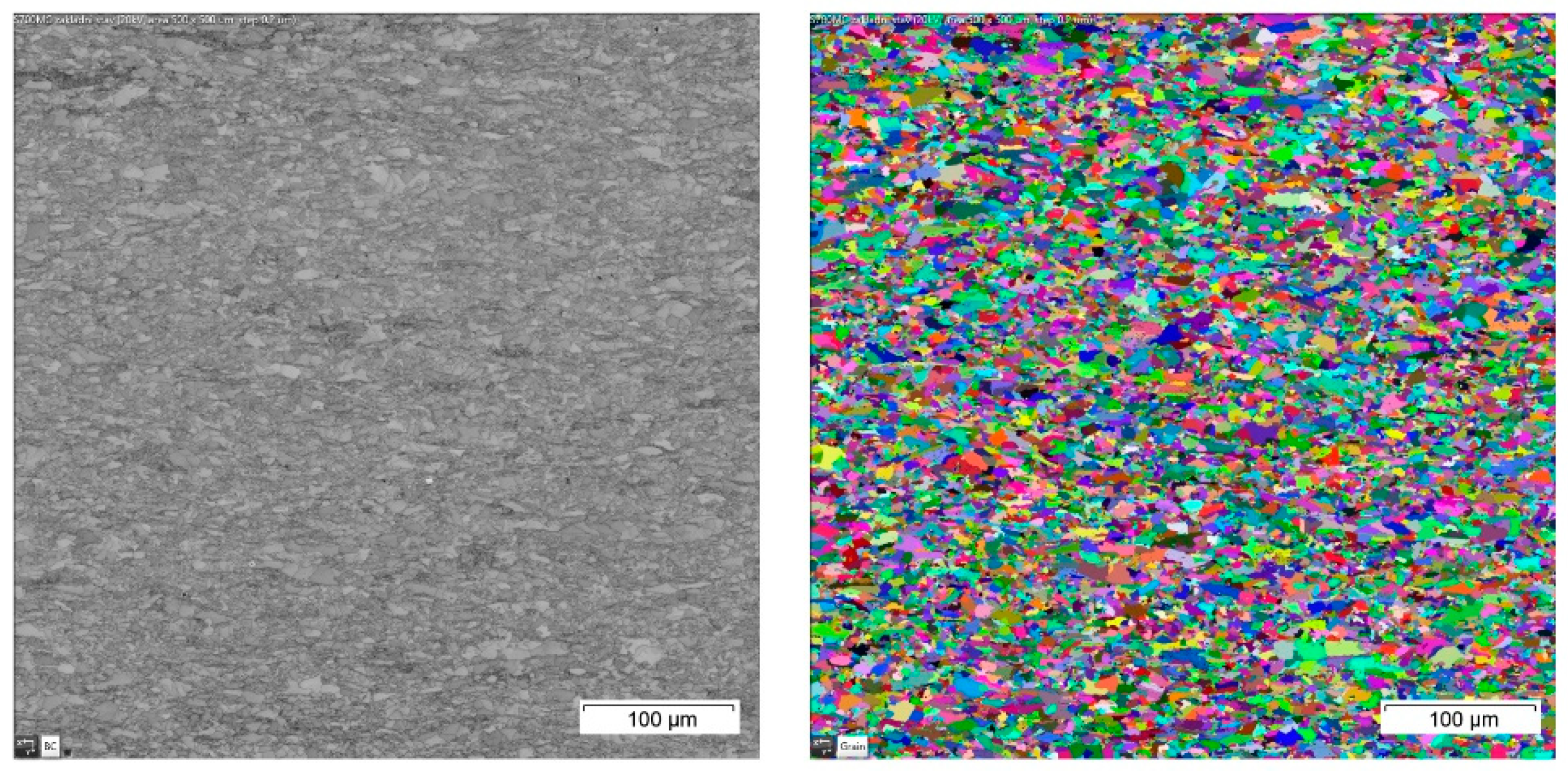
Figure 2.
Drawing of samples for dilatometric test.
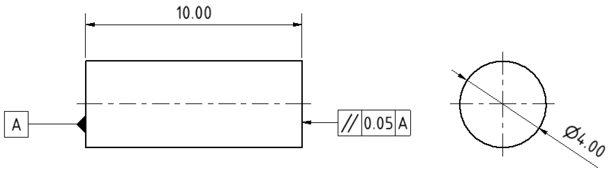
Figure 3.
Temperature cycles applied in dilatometer, heating phase (left) and cooling phase (right).
Figure 3.
Temperature cycles applied in dilatometer, heating phase (left) and cooling phase (right).
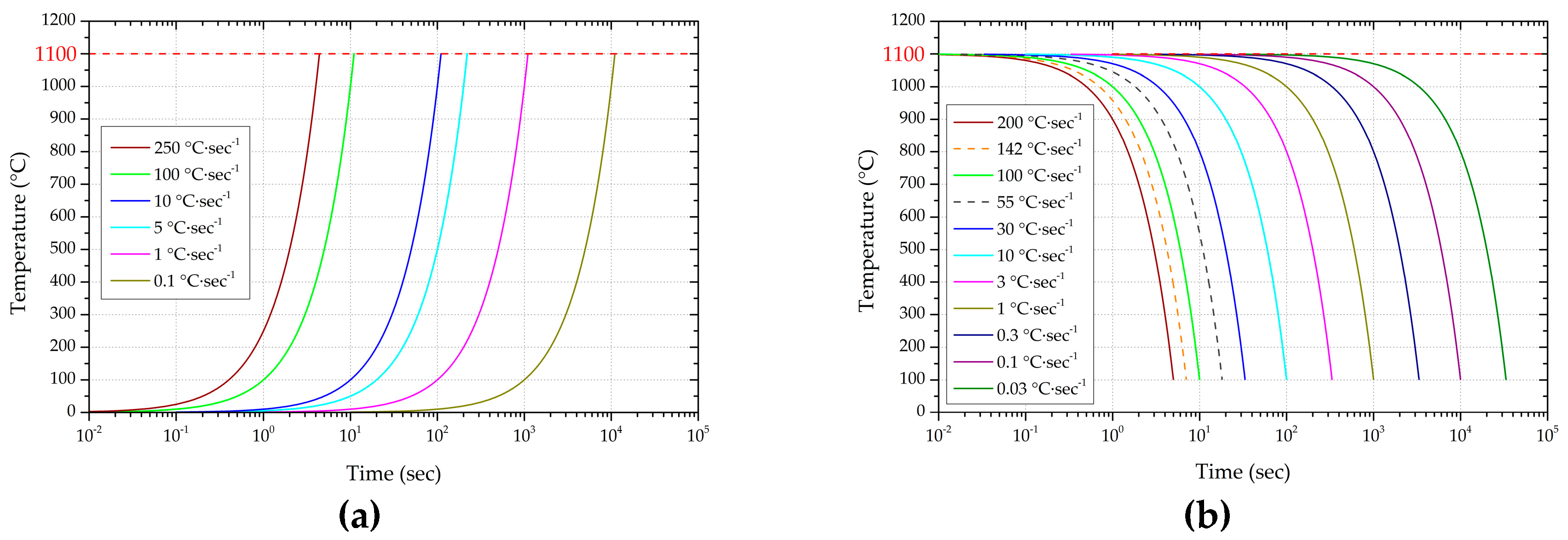
Figure 4.
The heating part of the dilatometry curve for heating rate 1 °C·sec-1 – evaluated by the method of three tangents.
Figure 4.
The heating part of the dilatometry curve for heating rate 1 °C·sec-1 – evaluated by the method of three tangents.
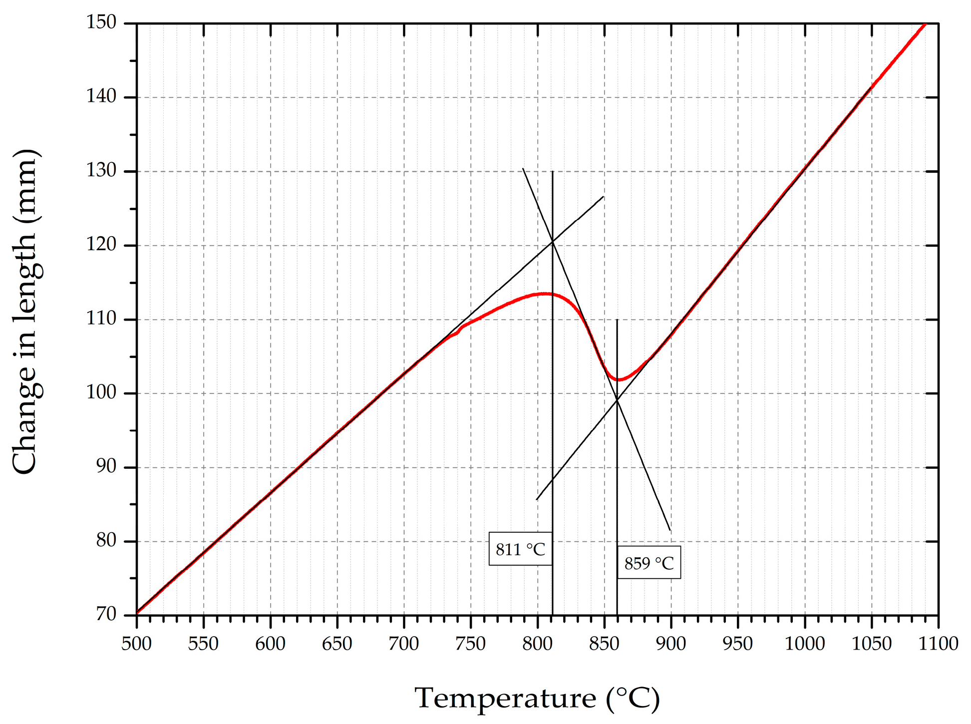
Figure 5.
The heating part of the dilatometry curve for 1 °C·sec-1 heating rate – evaluated by the first derivative method.
Figure 5.
The heating part of the dilatometry curve for 1 °C·sec-1 heating rate – evaluated by the first derivative method.
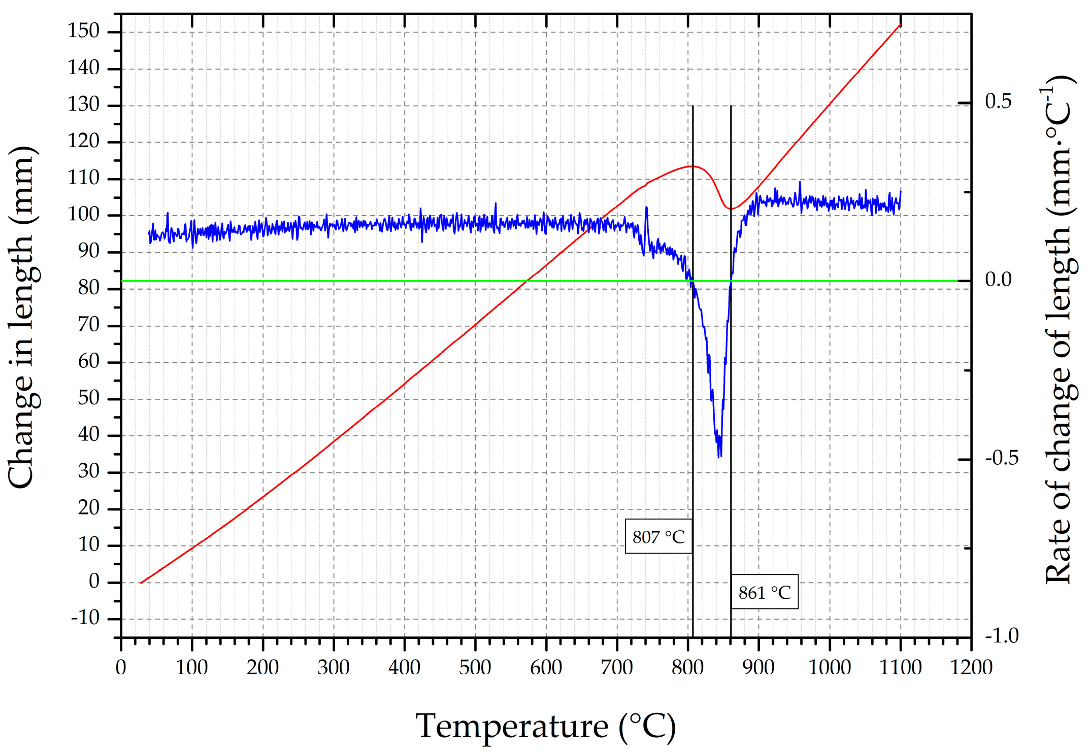
Figure 6.
The influences of the heating rate on the shift of the transformation temperatures Ac1 and Ac3.
Figure 6.
The influences of the heating rate on the shift of the transformation temperatures Ac1 and Ac3.
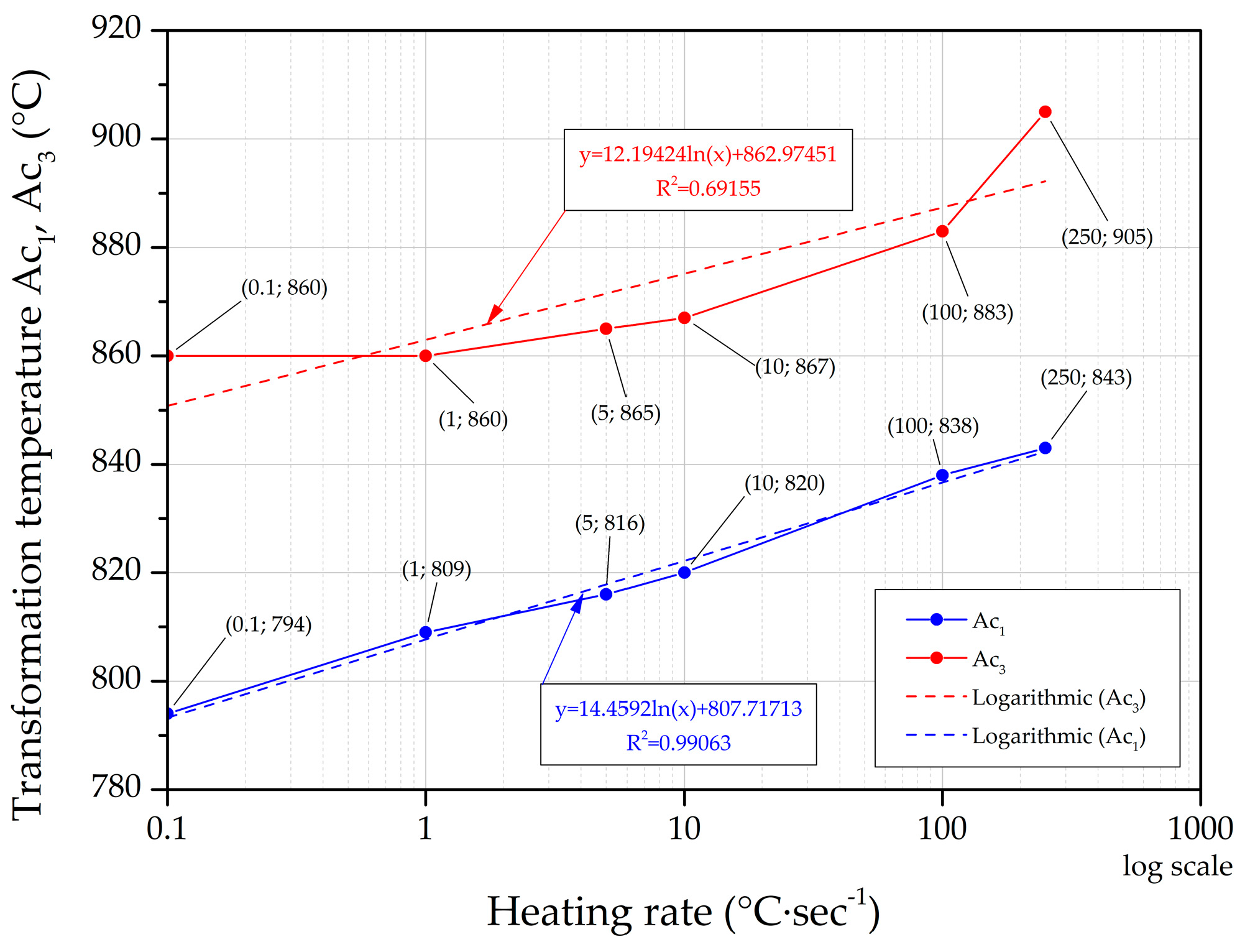
Figure 7.
Change in austenitization bandwidth as a function of heating rate.
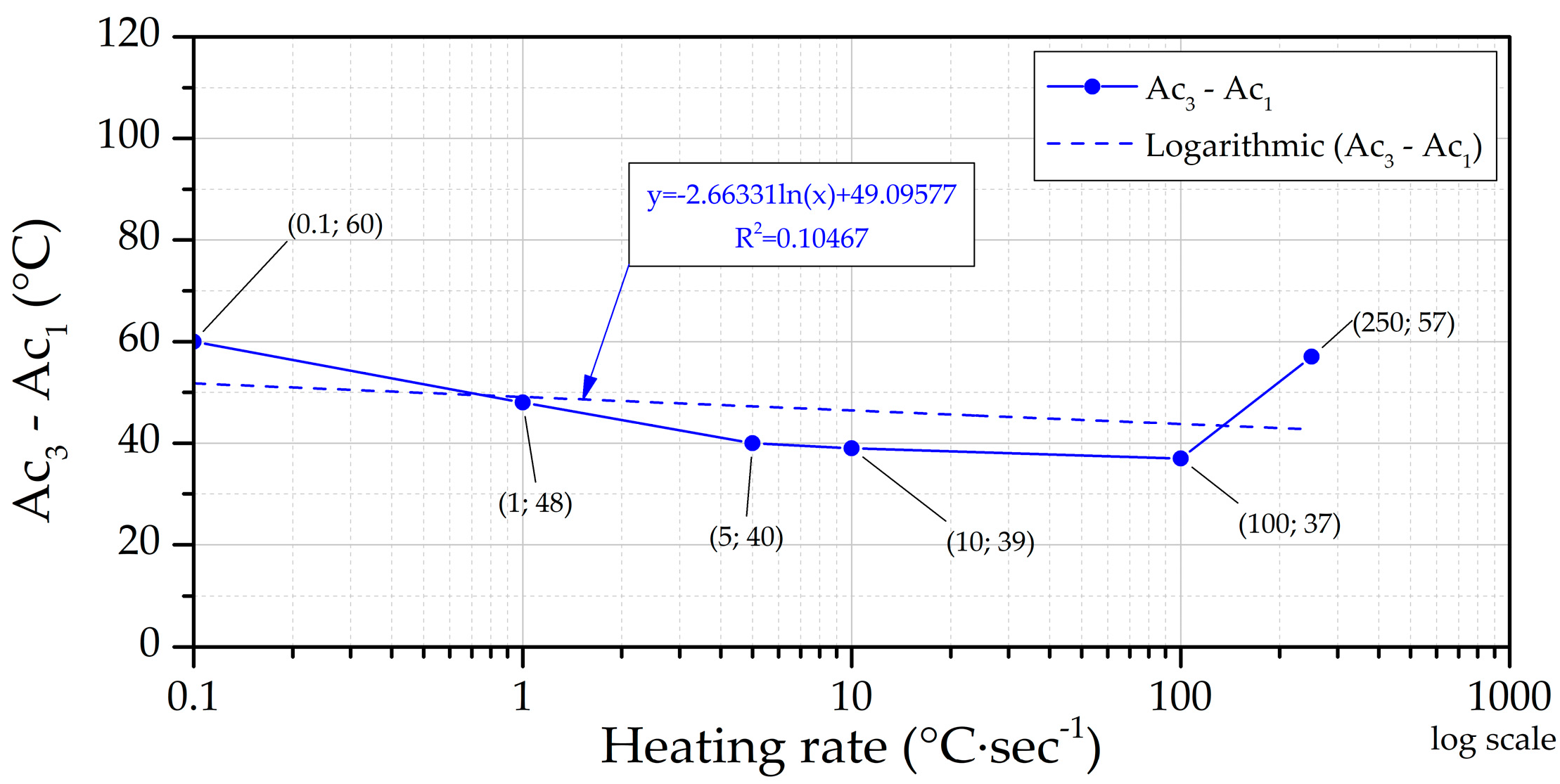
Figure 8.
Effect of cooling rate on the values of the beginning and end of the phase transformation – first derivation method (left) and three tangents method (right).
Figure 8.
Effect of cooling rate on the values of the beginning and end of the phase transformation – first derivation method (left) and three tangents method (right).
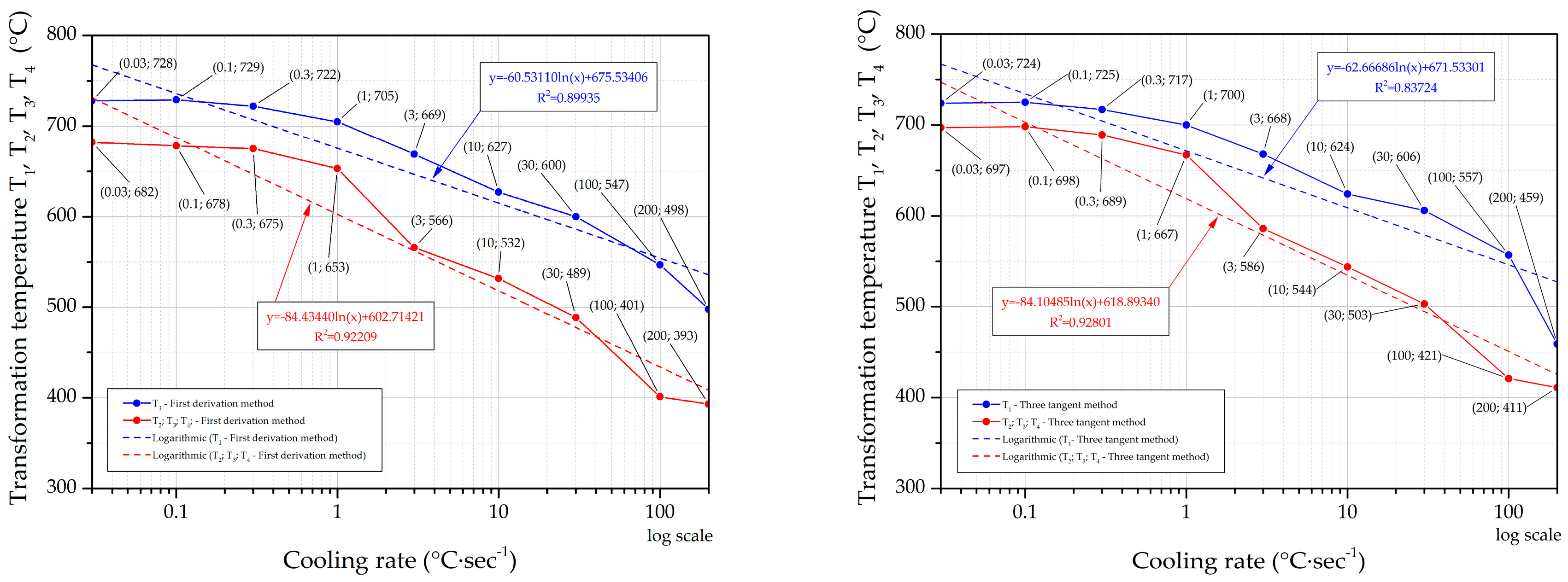
Figure 9.
Effect of cooling rates on material hardness values.
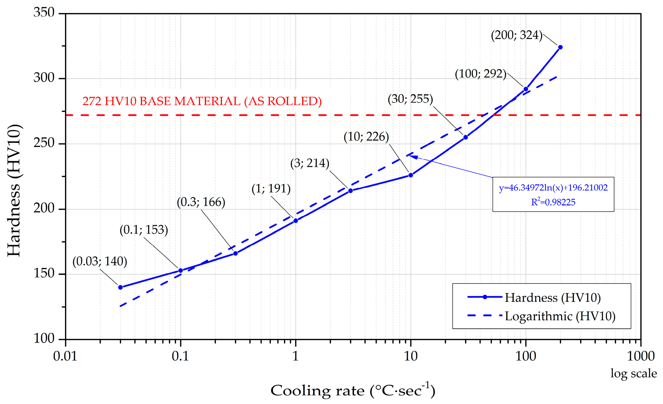
Figure 10.
Effect of cooling rate on the microstructure of S700MC.
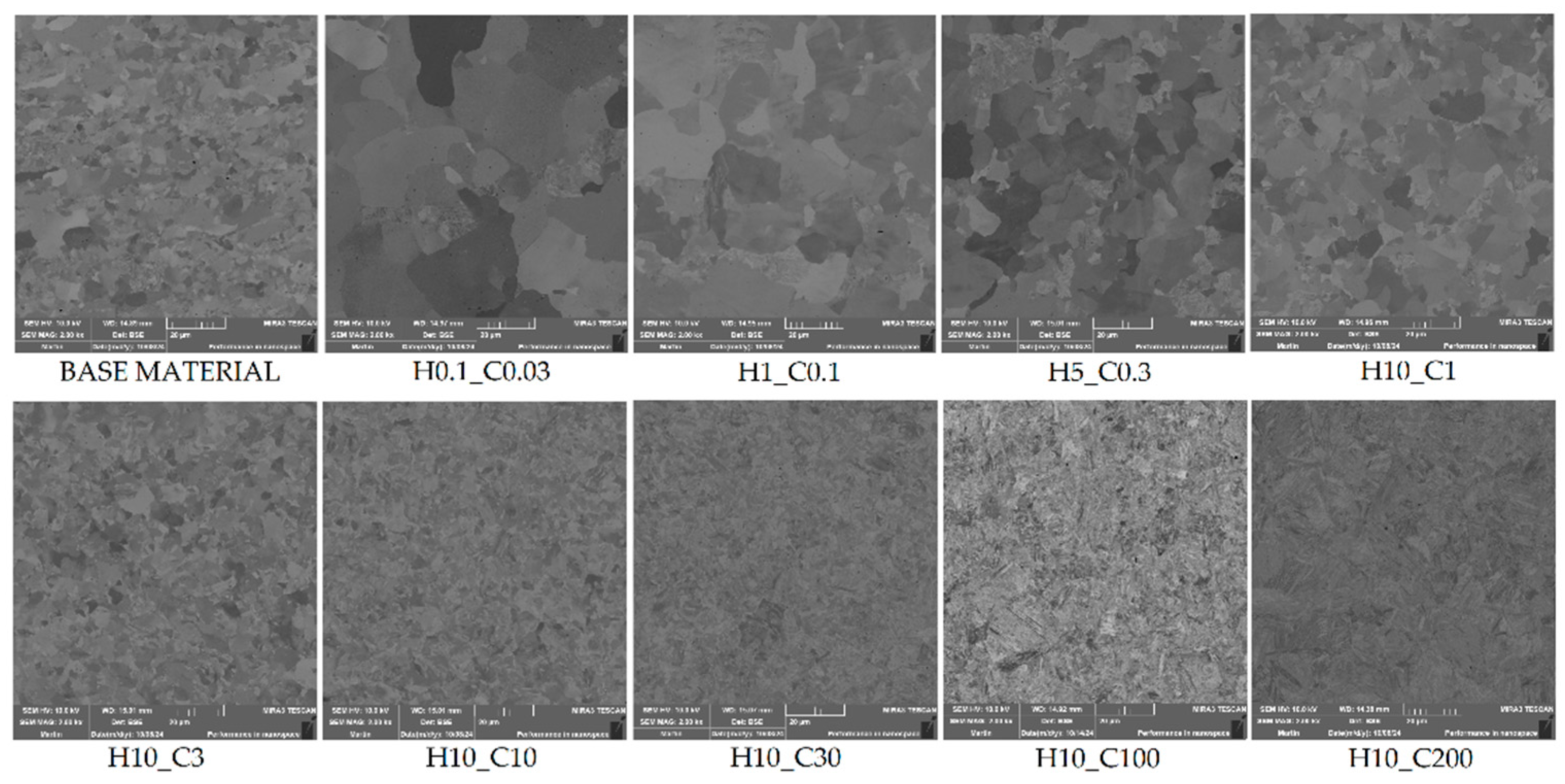
Figure 11.
The CCT diagram of S700MC steel.
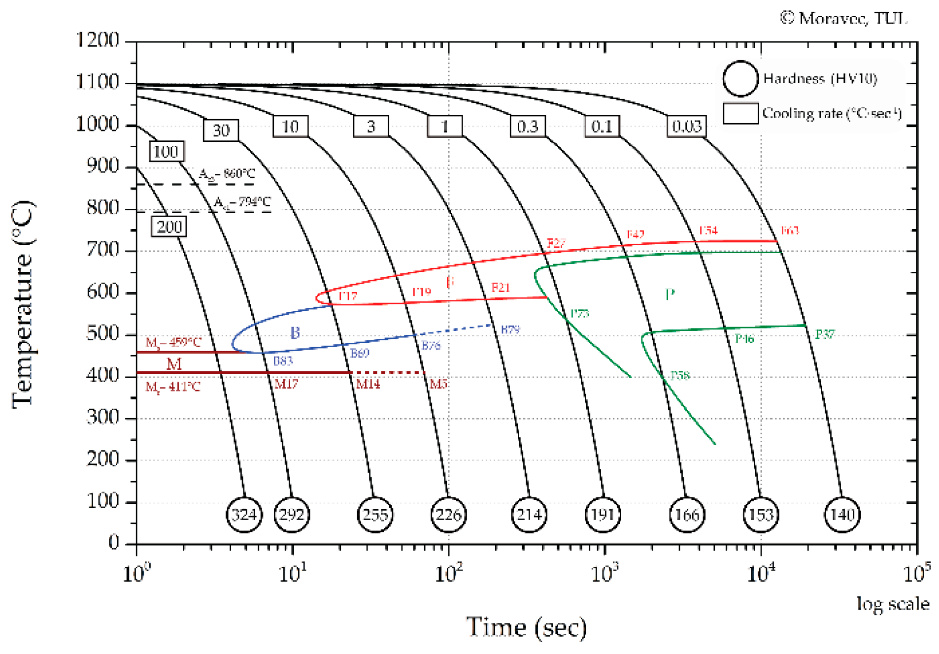
Figure 12.
EBSD analysis of grain size at different variants of the heating and cooling rates.
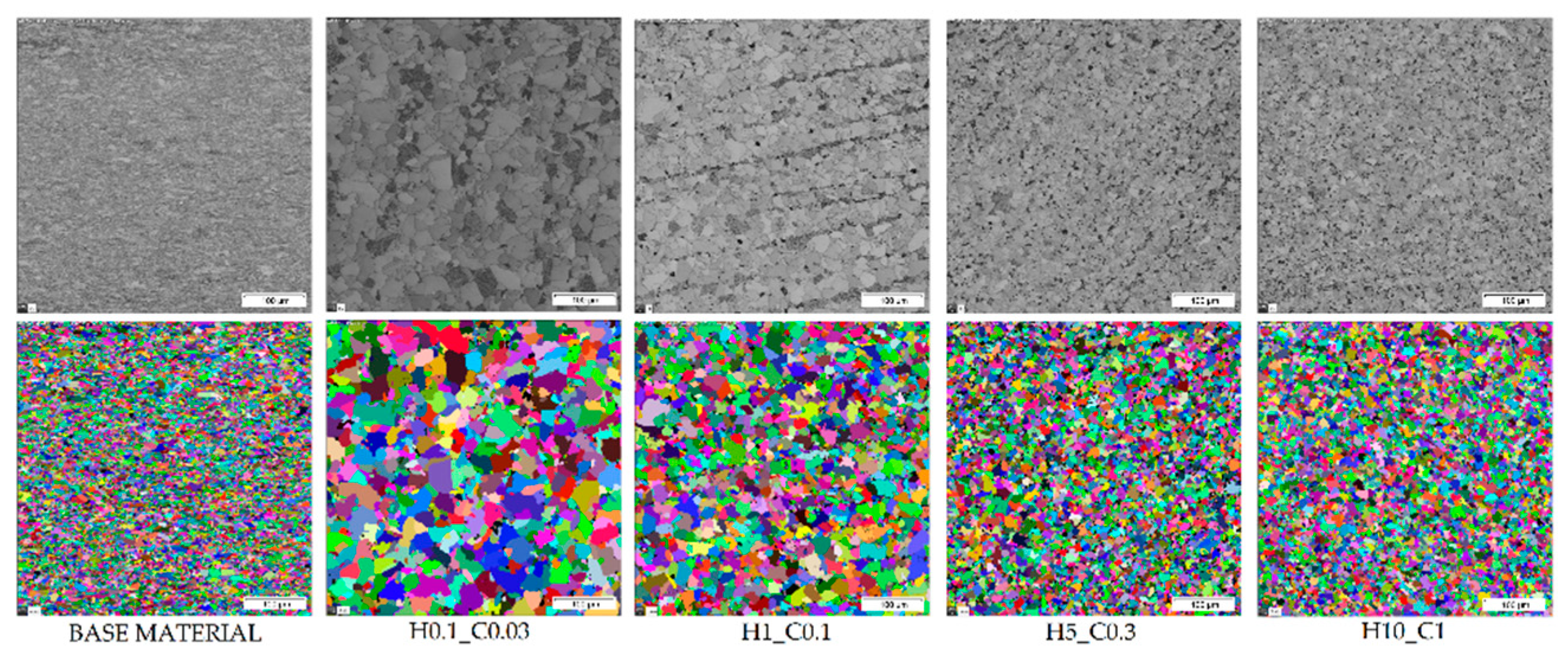
Figure 13.
The resulting grain size values for different combinations of heating and cooling rates.
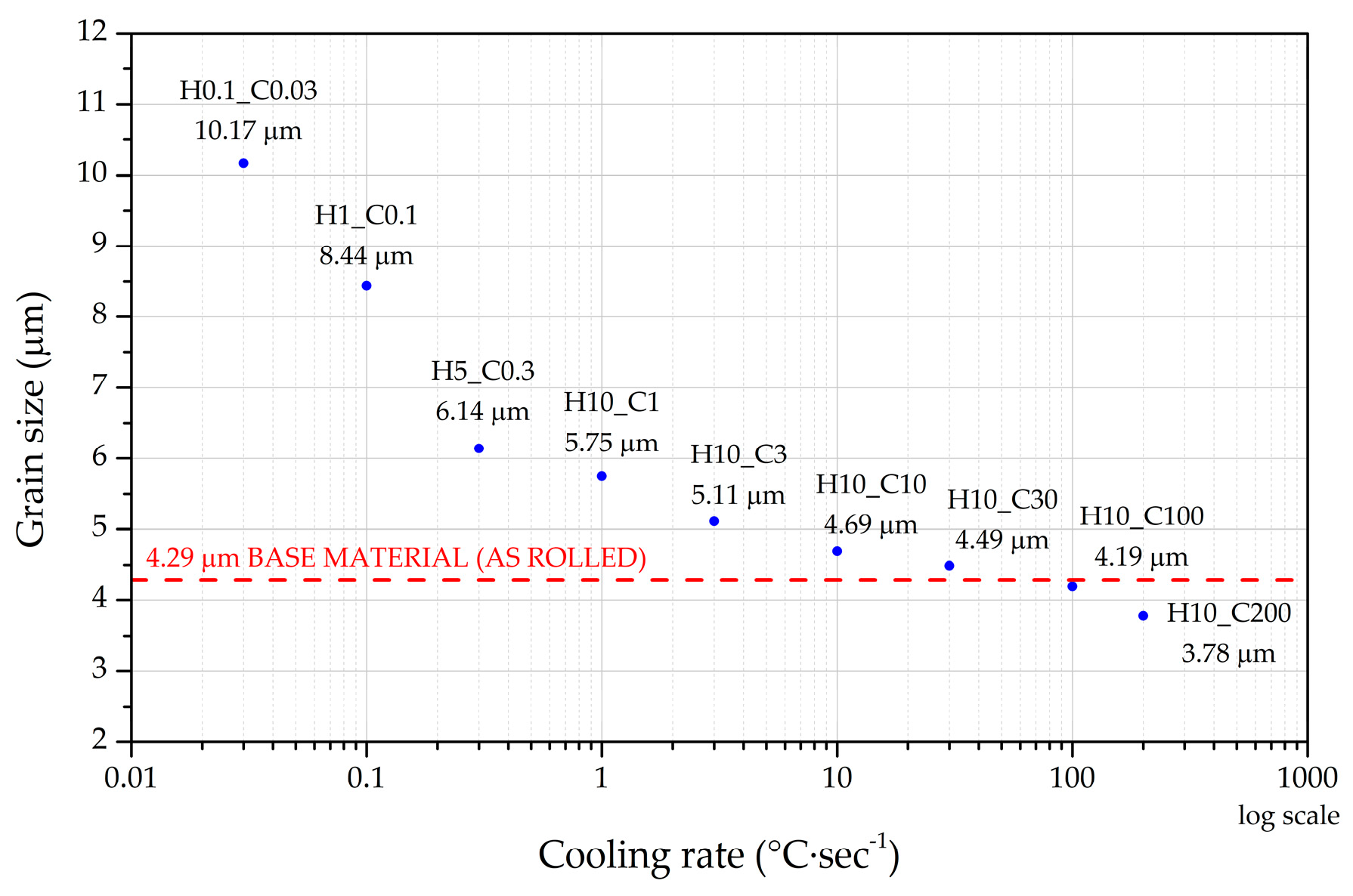

Table 1.
Chemical composition of S700MC steel (wt%).
| Element | C | Si | Mn | P | S | Al | Nb | V |
|---|---|---|---|---|---|---|---|---|
| EN 10149-2 | max. 0.12 | max. 0.6 | max. 2.2 | max. 0.025 | max. 0.010 | min. 0.015 | max. 0.09 * | max. 0.2 * |
| Experiment | 0.060 | 0.193 | 1.920 | 0.005 | 0.006 | 0.041 | 0.067 | 0.074 |
| Element | Ti | Mo | N | Ni | Cr | W | - | - |
| EN 10149-2 | max. 0.25 * | - | - | - | - | - | - | - |
| Experiment | 0.061 | 0.115 | 0.014 | 0.142 | 0.039 | 0.041 | - | - |
* Total content of Nb, V, Ti should not exceed max. 0.22 %.
Table 2.
Mechanical properties of S700MC steel.
| PYS (MPa) | UTS (MPa) | Ag (%) | A40mm (%) | |
|---|---|---|---|---|
| Average values | 738 ± 7 | 853 ± 3 | 11.34 ± 0.61 | 24.41 ± 0.52 |
Table 3.
Temperature cycles for determining transformation temperatures Ac1 and Ac3 and for assessing the effect of heating rate on the shift of them.
Table 3.
Temperature cycles for determining transformation temperatures Ac1 and Ac3 and for assessing the effect of heating rate on the shift of them.
| Variant Designation | H0.1_C10 | H1_C10 | H5_C10 | H10_C10 | H100_C10 | H250_C10 |
|---|---|---|---|---|---|---|
| Heating rate (°C·sec-1) | 0.1 | 1 | 5 | 10 | 100 | 250 |
| Cooling rate (°C·sec-1) | 10 | 10 | 10 | 10 | 10 | 10 |
Table 4.
Selected variations of temperature cycles for determining microstructures after austenite transformation during cooling.
Table 4.
Selected variations of temperature cycles for determining microstructures after austenite transformation during cooling.
| Variant Designation | H10_C0.03 | H10_C0.1 | H10_C0.3 | H10_C1 | H10_C3 | H10_C10 |
|---|---|---|---|---|---|---|
| Heating rate (°C·sec-1) | 10 | 10 | 10 | 10 | 10 | 10 |
| Cooling rate (°C·sec-1) | 0.03 | 0.1 | 0.3 | 1 | 3 | 10 |
| Variant Designation | H10_C30 | H10_C55* | H10_C100 | H10_C142* | H10_C200 | |
| Heating rate (°C·sec-1) | 10 | 10 | 10 | 10 | 10 | |
| Cooling rate (°C·sec-1) | 30 | 55 | 100 | 142 | 200 |
* Only to verify the occurrence of the phases in a specific part of the CCT diagram.
Table 5.
Selected variations of temperature cycles to assess the effect of heating and cooling rates on the resulting average grain size – EBSD analysis of samples.
Table 5.
Selected variations of temperature cycles to assess the effect of heating and cooling rates on the resulting average grain size – EBSD analysis of samples.
| Variant Designation | H0.1_C0.03 | H1_C0.1 | H5_C0.3 | H10_C1 | H10_C3 |
|---|---|---|---|---|---|
| Cooling rate (°C·sec-1) | 0.03 | 0.1 | 0.3 | 1 | 3 |
| Heating rate (°C·sec-1) | 0.1 | 1 | 5 | 10 | 10 |
| Variant Designation | H10_C10 | H10_C30 | H10_C100 | H10_C200 | |
| Cooling rate (°C·sec-1) | 10 | 30 | 100 | 200 | |
| Heating rate (°C·sec-1) | 10 | 10 | 10 | 10 |
Table 6.
Evaluation of the effect of different temperature cycles on the shift of transformation temperatures Ac1 a Ac3.
Table 6.
Evaluation of the effect of different temperature cycles on the shift of transformation temperatures Ac1 a Ac3.
| Variant Designation | H0.1_C0.03 | H1_C0.1 | H5_C0.3 | H10_C1 | H10_C3 | H10_C10 | |
|---|---|---|---|---|---|---|---|
| Heating Rate (°C·sec-1) | 0.1 | 1 | 5 | 10 | 100 | 200 | |
| Three tangents method (°C) | Ac1 | 796 | 811 | 823 | 826 | 844 | 844 |
| Ac3 | 856 | 859 | 863 | 865 | 881 | 901 | |
| First derivation method (°C) | Ac1 | 792 | 807 | 809 | 813 | 832 | 842 |
| Ac3 | 863 | 861 | 867 | 868 | 885 | 909 | |
| Differences between used methods (%) |
Ac1 | 0.50 | 0.49 | 1.70 | 1.57 | 1.42 | 0.24 |
| Ac3 | 0.81 | 0.23 | 0.46 | 0.35 | 0.45 | 0.88 |
Table 7.
Evaluation of transformation temperatures for the creation of the CCT diagram.
| Variant Designation | H0.1_C0.03 | H1_C0.1 | H5_C0.3 | H10_C1 | H10_C3 | H10_C10 | H10_C30 | H10_C100 | H10_C200 | |
|---|---|---|---|---|---|---|---|---|---|---|
| Cooling Rate (°C·sec-1) | 0.03 | 0.1 | 0.3 | 1 | 3 | 10 | 30 | 100 | 200 | |
| Three tangents method (°C) |
T1 | 724 | 725 | 717 | 700 | 668 | 624 | 606 | 557 | 459 |
| T2 | 697 | 698 | 689 | 667 | 586 | 591 | 570 | 481 | 411 | |
| T3 | 523 | 516 | 509 | 531 | - | 576 | 503 | 421 | - | |
| T4 | - | - | 399 | 448 | - | 544 | 419 | 373 | - | |
| First derivation method (°C) |
T1 | 728 | 729 | 722 | 705 | 669 | 627 | 600 | 547 | 498 |
| T2 | 682 | 678 | 675 | 653 | 566 | - | - | - | 393 | |
| T3 | - | - | - | - | - | - | 489 | 401 | - | |
| T4 | - | - | - | - | - | 532 | - | - | - | |
| Differences between used methods (%) |
T1 | 0.55 | 0.55 | 0.69 | 0.71 | 0.15 | 0.48 | 1.00 | 1.80 | 7.83 |
| T2; T3; T4 | 2.15 | 2.87 | 2.03 | 2.10 | 3.41 | 2.21 | 2.78 | 4.75 | 4.38 |
Table 8.
The hardness of the base material and the resulting structures after application of different cooling rates.
Table 8.
The hardness of the base material and the resulting structures after application of different cooling rates.
| Variant Designation | Base Material | H0.1_C0.03 | H1_C0.1 | H5_C0.3 | H10_C1 | H10_C3 | H10_C10 | H10_C30 | H10_C100 | H10_C200 |
|---|---|---|---|---|---|---|---|---|---|---|
| Cooling Rate (°C·sec-1) | - | 0.03 | 0.1 | 0.3 | 1 | 3 | 10 | 30 | 100 | 200 |
| Measured Hardness (HV10) | 270 | 141 | 154 | 165 | 192 | 211 | 227 | 254 | 287 | 319 |
| 271 | 138 | 154 | 166 | 191 | 214 | 227 | 253 | 289 | 328 | |
| 273 | 139 | 152 | 165 | 190 | 216 | 226 | 255 | 286 | 324 | |
| 270 | 139 | 152 | 167 | 189 | 216 | 227 | 255 | 297 | 326 | |
| 275 | 141 | 151 | 165 | 192 | 214 | 225 | 255 | 302 | 318 | |
| 273 | 142 | 154 | 166 | 190 | 213 | 225 | 255 | 292 | 324 | |
| 272 | 140 | 152 | 165 | 193 | 216 | 225 | 253 | 287 | 320 | |
| 271 | 141 | 152 | 165 | 191 | 214 | 227 | 256 | 286 | 328 | |
| 273 | 140 | 154 | 167 | 192 | 216 | 224 | 256 | 299 | 330 | |
| Mean Hardness (HV10) | 272.0 | 140.1 | 152.8 | 165.7 | 191.1 | 214.4 | 225.9 | 254.7 | 291.7 | 324.0 |
| Standard Deviation (HV10) | 1.6 | 1.2 | 1.1 | 0.8 | 1.2 | 1.6 | 1.1 | 1.1 | 5.8 | 4.1 |
Table 9.
Effect of cooling rates on average grain size.
| Variant Designation | Cooling Rate (°C/s) | Grain Size ECD (µm) Area 500 x 500 µm, Step Size 0.2 µm Average Value/Standard Deviation |
|---|---|---|
| H0.1_C0.03 | 0.03 | 10.17/9.09 |
| H1_C0.1 | 0.1 | 8.44/6.05 |
| H5_C0.3 | 0.3 | 6.14/3.44 |
| H10_C1 | 1 | 5.75/3.17 |
| H10_C3 | 3 | 5.11/2.65 |
| H10_C10 | 10 | 4.69/2.36 |
| H10_C30 | 30 | 4.49/2.42 |
| H10_C100 | 100 | 4.19/2.11 |
| H10_C200 | 200 | 3.78/1.69 |
| Base Material (As Rolled) | - | 4.29/2.03 |
Disclaimer/Publisher’s Note: The statements, opinions and data contained in all publications are solely those of the individual author(s) and contributor(s) and not of MDPI and/or the editor(s). MDPI and/or the editor(s) disclaim responsibility for any injury to people or property resulting from any ideas, methods, instructions or products referred to in the content. |
© 2024 by the authors. Licensee MDPI, Basel, Switzerland. This article is an open access article distributed under the terms and conditions of the Creative Commons Attribution (CC BY) license (http://creativecommons.org/licenses/by/4.0/).
Copyright: This open access article is published under a Creative Commons CC BY 4.0 license, which permit the free download, distribution, and reuse, provided that the author and preprint are cited in any reuse.


