Submitted:
25 November 2024
Posted:
26 November 2024
You are already at the latest version
Abstract
The rate of evolution plays a crucial role in understanding the pace at which species evolve.
Various statistical models have been developed to estimate the rate parameters for a group of related species evolving along a phylogenetic tree.
Existing models often assume the independence of the rate parameters;
however,
this assumption may not account for scenarios where the rate of evolution correlates with its evolutionary history.
We propose using the autoregressive-moving-average (ARMA) model for modeling the rate of evolution along the tree,
hypothesizing that rates between two successive generations (ancestor-descendant) are time dependent and correlated along the tree.
We denote \texttt{phyrateARMA}$(p,q)$ as a phylogenetic ARMA($p$,$q$) model in our innovation.
Our algorithm begins by utilizing the tree and trait data to estimate the rates on each branch,
followed by implementing the ARMA process to infer the relationships between successive rates.
We apply our innovation to analyze the primate body mass dataset and plant genome size dataset and test for the autoregressive effect of rate of evolution along the tree.
Keywords:
Autoregressive moving average model
; evolutionary rates
; phylogenetic comparative method
; Brownian motion
; trait evolution
1. Introduction
In evolution, studying the heritable characteristics of the biological population is helpful to understand the diversity between species on our planet Earth [1]. Macroevolution is expected to occur when selection acts on a trait that has a heritable basis of phenotypic variation. During the evolutionary process, speciation results in new species, and the comparison of traits (e.g. height, weight, size, ⋯ etc.) among a group of related species can be made by studying the speed of changes in their characteristics over successive generations [2].
Although one subgroup of species evolved at a faster rate and resulted in a larger variation in the trait, the other subgroup of species evolved at a relatively lower rate and produced a moderate variation of the trait. When evolutionary processes such as natural selection (including sexual selection) and genetic drift act on this variation, certain characteristics become more common or rare within a population [3]. For example, Darwin finches are a group of about 18 species of dull-colored passerine birds on the Galápagos islands [4]. They are well known for their remarkable diversity in form, size, and function of the beak, which is highly adapted to different food sources [5]. Another example is angiosperms, which survive and thrive successfully on our planet. The evolution of fruits is one of the most important characteristics, as fruits not only provide a food source for other species, but also protect seeds and contribute to seed dispersal [6]. The survival and success of fruits require adaptation to their environment. For example, while dragon fruit (Selenicereus) endures temperatures up to 40°C (104°F) for survival, watermelon (Citrullus lanatus) needs temperatures higher than about 25°C (77°F) to thrive. Studying the reproducible properties by the rate of evolution to the resistance of temperature would help us shed light on the evolution of angiosperms themselves and understand their ecological implications.
The rate of evolution is a measurement of the change in an evolutionary lineage over time and can be defined as the ratio of the character displacement over a certain time interval. [7] defined the rate of change between two samples using three quantities: the proportional difference between the sample means, the pooled standard deviation of the samples, and the time interval between the samples. For example, suppose that a character has been measured twice, and , where and are expressed as the time before the present in millions of years. The time interval between the two samples can be written as , which is 1 million years if and . The average value of the character is defined as in the previous sample and in the later sample. Let be the natural logarithm taking into account and . Then the evolutionary rate () can be defined as in Eq. (1)
Next, multiplying the time difference on both sides of Eq. (1) produces the character difference within a time unit Conceptually consider that the character change occurred in infinitesimal time and denote the character displacement by , then we have the differential equation . Given , the solution is which shows that increased with time t. Unfortunately, this may not be an appropriate model for describing character change in the evolutionary perspective. Instead, one may consider that the variation of the character change adopts a certain dynamic. For example, if one considers that the variation of the character change is proportional to time, then a stochastic variable can be introduced, where is a Wiener process with independent Gaussian distributed increment and is a normal distributed random variable with mean 0 and variance (i.e. ). Thus, the displacement of the continuous trait variable () solves stochastic differential equation shown in Eq. (2)
Given , integrate both sides of Eq. (2), one has
where , and .
Given the initial value , Eq. (3) describes the dynamic of the trait variable at time t pending the rate parameter . Figure 1 presents one hundred trajectories generated using rates (bottom left) and (bottom right), respectively. It can be seen straightforwardly that while a smaller rate () yields a narrower range of character value, the larger rate () yields a wider range of character value.
For a group of n related species, denote as the trait variable for the ith species. Then we can apply the Brownian motion with the rate parameter to explore the dynamic of the trait along the evolutionary history using a phylgoenetic tree that represents the relatedness between species. In particular, the estimation of the evolution rate can be performed using comparative phylogenetic methods (PCM) [8,9,10].
There are models created on the basis of Eq. (3) via considering the constant-rates BM model may not be well addressed for the evolution in many scenarios [11,12,13,14,15]. Those models come with the assumption that the evolution of a species changes over time, the rates of evolution can be modeled as either constants or stochastic variables along times (branch lengths). The trait variable adopts the following dynamics.
where can be constant (i.e. ) [16], piecewise constant (i.e. where and are the successive time regimes) [11] or a random variable modeled by another pertinent process (i.e. where is a distribution function for the stochastic variable) [17,18].
A hypothetical tree of four species and the corresponding simulation of the trajectories s using Brownian motion along a rooted phylogenetic tree under two different rates is shown in Figure 2.
Those models have been broadly applied in many studies. For example, in the evolution of the morphology of the world’s largest flowers (Raffkesianeae: up to 1 meters in diameter), [19] found that the enormous flowers evolved from ancestors with tiny flowers. In the study of the evolution of the size of the plant genome, [20] found that the woody lineages had a stochastic motion rate that was nearly five times slower than the rate of the herbaceous lineages. Although the existing framework has produced rate models, none consider a scenario in which the rate is treated as a time-correlated stochastic variable, which could potentially enhance the study of rate evolution. This highlights the need for our work to apply a time series model [21,22]. Specifically, this approach aims to answer key questions: Are the evolutionary rates of biological traits statistically independent, or are they believed to be phylogenetically serially autocorrelated ?
Note that in modeling the rate of evolution, it is essential to consider its dynamic nature, as the rate can fluctuate, increase, or decrease over time [18,23], rather than a constant. Consider that the implementation of the time-correlated rate evolution could possibly provide an alternative to reveal embedded information about species evolution, in this work we intend to expand the model in Eq. (4) within the framework of correlated rate evolution ( for where is a parameter vector) to model the trait evolution for phylogenetic comparative analysis. In particular, we use the autoregressive moving average (ARMA) time series model that has been widely applied in econometrics to model the rate parameter [24,25]. The description of the methods can be found in Section 2. The simulations are detailed in Section 3. Empirical analyzes are presented in Section 4. The discussions and conclusions are covered in Section 5.
2. Methods
2.1. Trait Evolution with Time Correlated Rate
We describe our procedure as follows. In Section 2.1.1, we adopt phylogenetic ridge regression [26] to perform the analysis using the phylogenetic tree and trait data as input to obtain rate estimates. In Section 2.1.2, we perform a phylogenetic rate ARMA(p,q) regression, w here the rate estimates are incorporated along the tree using a traversal algorithm, treating the data as time series.
2.1.1. Step 1: Phylogenetic Ridge Regression
Given the tree with the topology and branch lengths, one assumed that the observed trait values are a linear combination of past values, the time elapsed, and the rate of evolutionary change. To illustrate, we use a case of 3 taxa tree as shown in Figure 3 where the extant species A, B, and C, and the fossil species D, E, and O have trait values of and . These traits values can be expressed as a linear combination of the time elapsed and the rate of evolution shown in Eq. (5).
One can formulate into the system of linear equation in Eq. (6)
Given empirical data where the tip values are , , and , and the ancestral values and may be known through fossil records or remain unknown. Assuming the currently provided data , and the phylogenetic tree with a given set of known branch lengths , the tip states can be written into a matrix form in Eq. (7)
In general, given tip data , and tree topology of n taxa with branch length set where is internal node index set with the corresponding with the ancestral-descedant relationship delineated by the tree topology, we use the R package rrphylo [27] to perform the analysis for estimation of phenotypic evolutionary rates using Eq. (10) with adopting the leave-one-out cross-validation (LOOCV) to search for the optimal . In this method, each observation is removed one at a time, and the remaining data is used to make predictions. The error for the excluded observation is calculated, and this process is repeated for all observations. The total LOOCV error is computed for various values, and the with the smallest error is selected as the best regularization parameter, improving model performance [26].
2.1.2. Step 2: Phylogenetic Rate ARMA(p,q) for Trait Evolution
Next, we implements the ARMA model for studying rate . Given tree topology of n taxa and with tip node and internal node index set and the corresponding branch length set with the ancestral-descedant relationship delineated by the tree topology, by utilizing phylogenetic ridge regression in Eq. (10) one can get a set of estimated rates where index corresponds to the internal index, then the phylogenetic ARMA() model of rates defined by a mixture of phylogenetic autoregressive (AR) and phylogenetic moving average (MA) models given by the Eq. (11):
where represents the time series at time , are coefficients for the AR terms, are coefficients for the MA terms, and denotes the white noise error terms following a normal distribution with mean zero and variable proportional to the branch length as shown in Eq. (12)
For a phylogenetic ARMA(1,1) rate model, denote as the descendent () and as the ancestor, the model in Eq. (11) can be represented as in Eq. (13).
An exemplary example of the 3 taxa case is shown in Figure 4.
We are interested in the joint distribution where is the parameter vector (i.e. for the ARMA . On a specific branch with branch length , we assume the error follow a normal distribution with mean conditioning on the ancestor and variance with branch length . The logarithmic likelihood on a branch is a one- dimensional ARMA that has likelihood in Eq. (14).
Assuming branches are independent, the full log likelihood given the tree and trait , can be written as
where is the residual at the root and the product operator follows the corresponding tree topology .
To perform model inference on parameter estimation, given trait vector on the tip, and a phylogenetic tree with known branch length set where is the branch length of the root node, and each branch . Use y and the tree to obtain the rate estimates at the root from the Brownian motion model [12]
where is the MLE estimate for the ancestral at the root under the Brownian motion model, and is the variance covariance matrix transformed from the tree and 1 = (1, 1, ⋯, 1)t is vectors of 1s. Then we use the maximum likelihood approach for parameter estimation and inference. Refer to Section 6.2 Appendix for expression and parameter estimation a first few order phylorateARMA((p, q)) model.
For empirical analysis, we analyze the data using the model up to order . For model selection, the Akaike information criterion and its sample size correction version [28] and the weighted parameter are calculated using equation , where is the weight for the models i and . The weighted parameter estimate is calculated as . Here, represents the MLE estimate from model i. This method incorporates uncertainty in the selection of the model by averaging parameters based on AIC weights [29].
2.2. Testing of AR(1) Effect
We conduct inference to test for the existence of the autoregressive effect. This is equivalent to testing whether , as shown in Section 2.2.1. Additionally, we investigate whether the autoregressive effect varies across different clades of the tree. For this, we pose the null hypothesis , which is discussed in Section 2.2.2.
2.2.1. Test of Correlated Rate Evolution
Given the AR(1) process: where is white noise, the asymptotic variance of the MLE is: . The null hypothesis is given by: where is a hypothesized value. The alternative hypothesis for a two-sided test is: . We set to test for the AR(1) effect. To perform the test, first fit an AR(1) model to the data and obtain the estimate of and its standard error . The test statistic is calculated as:
This test statistic is compared with the critical value of the t distribution with degrees of freedom, where n is the sample size. The standard deviation estimate can be derived from the Hessian matrix obtained during the optimization process, which is then used to conduct hypothesis testing.
In the context of hypothesis testing for phylogenetic rate model in an AR(1) model, the process begins by establishing the null hypothesis, , where represents a specific hypothesized value. The alternative hypothesis for a two-sided test is . The methodology for testing these hypotheses involves several steps: (i) Firstly, an AR(1) model is fitted to the data. From this model, the estimate of and its standard error are obtained. (ii) The next step involves calculating the test statistic using the formula . (iii) Finally, this test statistic is compared against the critical value from the t-distribution, which is determined by the sample size where is the number of the branches of the tree and corresponds to degrees of freedom. This comprehensive method is essential to determine whether the hypothesized value is a plausible value for in the AR(1) model.
2.2.2. Testing Heterogeneity Rates on Sub Clade
We consider whether heterogeneity autoregressive effect exists on the two subclade, as shown in Figure 5.
The null Hypothesis () poses that a single tree with n taxa and use one parameter while the alternative Hypothesis () states that 2 autoregressive parameters and would more approporate when tree the is divided into two subtrees from the root, and parameters are estimated independently.
The null hypothesis in the likelihood ratio test states that the simpler model (in this case, the single combined tree) is sufficient to explain the variability in the data. The alternative hypothesis suggests that dividing the tree into two subtrees provides a better fit. The likelihood ratio test (LRT) statistic is computed as:
where is the log-likelihood under the null hypothesis and is the log-likelihood under the alternative hypothesis. The test statistic follows a chi-square distribution with the degrees of freedom .
The procedure in our framework is summarized in Algorithm 1.
| Algorithm 1: Procedure of Phylogenetic ARMA(p,q) Rate Data Analysis |
|
3. Simulation
We assess the performance of the model using simulation. Four types of trees are used for the assessment: star tree, balanced tree, left tree, coalescent tree, and birth-and-death tree, each of size . The initial samples are drawn from an independent normal distribution. The initial estimate for by applying the formula in Eq. (16) at the root is estimated by the Brownian motion model using the R package geiger. For each type of tree, for each data set and for each prior set, a million replicates of the sample will be generated to assess the posterior sample distribution.
Let the tree have m branches, with each branch representing a transition between an ancestral node and a descendant node . The tree is traversed in postorder (from root to tips), and the trait values for each node are computed based on the following AR(1) process.
For each branch, the evolutionary rate at the descendant node is determined by the rate at its ancestor , with some noise (innovation) added. The autoregressive equation is shown in Eq. (19)
Initially, the rate value at the root node is set to zero: .
After simulating the rates using Eq. (19) for all nodes in the tree, the final trait values at the tree tips (taxa) are computed by accumulating the rates along the path from the root to each tip.
Let denote the set of nodes from the root to tip j, and denote the branch length leading to node . The trait value at each tip j is:
where is the final accumulated trait value at tip j.
The final output consists of two arrays: (1) the array of simulated evolutionary rates for each node, , and (2) the trait values at the tree tips, summarized by the following equations Eq. (21)
This simulation captures the evolutionary rate changes along a phylogeny under an AR(1) model, accounting for both ancestral states and random innovation at each branch. We create a function simulate_trait_data_given_phi which simulates the trait evolution process along a phylogenetic tree using an autoregressive process (AR(1)) for the rates of evolution. The simulation setup is shown in Algorithm 2
| Algorithm 2: Estimating Type I Error and Power with Phylogenetic AR(1) rate Model |
|
Figure 6 and Table 1 show how the statistical power to detect an effect changes with different values of and different taxa levels.
From Figure 6 and Table 1, one can envision that the power of the test changes depending on the number of taxa. Generally, as the number of taxa increases, the power also increases. Next, for all taxa levels, as increases, the power of the test also increases. This could mean that as the parameter increases, the ability to detect an effect or a difference becomes stronger. Third, all curves converge or come closer together at higher values of , indicating that the power could be more consistent across different levels of taxa at these higher values. This simulation provide the evidence that our methods fit the statistical properties as expect in the performance of evaluating the statistical power and type I error.
4. Empirical Analysis
4.1. Genome Size Rate Evolution in Herbaticus and Woody Plant
This study collected and analyzed data sets on the genome size in pg of herbaticus and woody plant. The primary data source is [30], we includes 35 herbaticus and 33 woody species in this study. The main objective is to test whether there is a time-series relationship in the evolutionary rate of these plant’ genome size.
Figure 7 shows the phylgoenetic tree for herbaticus, woody and their joint tree.
4.1.1. Genome Size: Combined Herbaticus and Woody Species
Table 2 presents the parameter estimates for various autoregressive (AR) and autoregressive moving average (ARMA) models. ARMA(1,1) has a value of and a value of , indicating a moderate correlation between consecutive rates of evolution, with a residual variance of . The weighted estimates combine values across the models, with and , and , providing a comprehensive view of the underlying evolutionary process.
Using the phylogenetic ARMA(1,1) rate model described in Eq. (13), the equation for demonstrates how the descendant’s rate of evolution is influenced by multiple factors. The term indicates that -5.0% of the ancestor’s evolutionary rate () is carried over to the descendant, reflecting a weak and inverse correlation between the two rates. The second term, , with a coefficient of , adjusts for the random variation (or noise) in the ancestor’s rate. This positive value suggests that random fluctuations in the ancestor’s rate have a small reinforcing effect on the descendant. Finally, , with variance proportional to , represents the new random variation specific to the descendant. The weighted estimates offer a balanced perspective on how both inherited traits and random fluctuations shape evolutionary changes across generations.
In Table 3, AR(2) ranks first with the lowest AICc value of and the highest Akaike weight (), indicating the best fit among the models. AR(1) follows with an AICc of and a weight of , suggesting a close fit but slightly less optimal than AR(2). ARMA(1,1) ranks third with an AICc of and a weight of . Models ARMA(2,1) and ARMA(2,2) show considerably lower Akaike weights, indicating that increasing model complexity beyond AR(2) does not significantly improve the fit.
4.1.2. Genome Size: Herbaticus Species
The parameter estimates in Table 4 for the herbaticus models show that AR(1) has a value of with residual variance , indicating a moderate influence from the previous rate of evolution. AR(2) introduces a second autoregressive term () and maintains a similar variance of . The ARMA(1,1) model has and , with the same variance of . More complex models, such as ARMA(2,1) and ARMA(2,2), show mixed and values, but they maintain the same low variance of .
The weighted estimate balances these models, showing , , and . This suggests that the descendant’s rate of evolution is influenced by % of the ancestor’s rate, with a small adjustment of % due to noise from the ancestor, all within a low variance process.
In Table 5, AR(1) ranks first with the lowest AICc value of and the highest Akaike weight (), making it the best-fitting model for the herbaticus data. ARMA(1,1) follows in second place with an AICc of and a weight of , while AR(2) ranks fourth with an AICc of and a weight of . More complex models like ARMA(2,1) and ARMA(2,2) have even lower Akaike weights, indicating that they provide little additional explanatory power compared to simpler models.
4.1.3. Genome Size: Woody Species
The parameter estimates in Table 6 for the woody models indicate that AR(1) has a value of and a residual variance of , suggesting a very weak negative influence from the previous rate of evolution. AR(2) introduces a second autoregressive term () and slightly increases the variance to . ARMA(1,1) shows stronger dependence with and , while maintaining a variance of .
The weighted estimate balances the models, with , , and . This suggests that the descendant’s rate is slightly positively influenced by the ancestor’s rate (%) but slightly negatively impacted by the noise (%), with very low overall variance (), indicating minimal change between generations.
In Table 7, AR(1) ranks first with the lowest AICc value of and the highest Akaike weight (), indicating it is the best-fitting model for the woody data. ARMA(1,1) ranks second with an AICc of and a much smaller weight (), while AR(2) ranks last with an AICc of and no Akaike weight (). More complex models, such as ARMA(2,1) and ARMA(2,2), also have minimal Akaike weights (), suggesting they provide little additional explanatory power and overcomplicate the fit for the woody data.
From above one may foreseen that the woody primate and the herbaticus genome size possess different autoregressive effect for the rates of the evolution, we provide the test in the following sections.
4.1.4. Testing Autocorrelation Rate
Interpretation of AR(1) Test Results
Table 8 show the AR1 test result
Table 8 presents the results of the AR(1) test under the null hypothesis (no autocorrelation) and the alternative hypothesis . The herbaticus tree shows a significant positive autocorrelation with a large z-value of 5.100 and a p-value of 0.000, strongly rejecting the null hypothesis. This suggests a significant effect of the previous rate of evolution on the current rate in the herbaticus dataset.
In contrast, the woody tree show no significant autocorrelation, with z-values of , and p-value indicates that the null hypothesis cannot be rejected for these datasets, suggesting no significant relationship between the past and current rates of evolution in the woody trees. This may due to woody tree with slower rates (5 times slower than the herbaticus tree [20]).
The combined tree shows no significant autocorrelation, with z-values of , and p-values of . The result suggests that there is no significant relationship between the past and current rates of evolution in the combined trees.
Testing Heterogeneity Rates on subclades
Table 9 presents the results of the heterogeneity test in evolutionary rates across the herbaticus, woody, and combined (dino) subclades using various autoregressive models (AR(1), AR(2), ARMA(1,1), ARMA(2,1), ARMA(2,2)). The log-likelihood values for the herbaticus (), woody (), and combined () datasets are provided, along with the chi-squared statistic and p-values.
All models yield highly significant results (p-values = 0.00), indicating strong evidence for rate heterogeneity between the subclades. The highest chi-squared statistic is observed for AR(1) (847.16), suggesting that it explains the greatest amount of variance in the data compared to the other models.
4.2. Body Mass Rate Evolution in Diurnal and Nocturnal Primate
This study collected and analyzed data sets on the body weights of male and female primates. The primary data source are [33] and Animal Diversity Web [34], which includes diurnal and nocturnal male and female primates. The main objective is to test whether there is a time-series relationship in the evolutionary rate of these primates’ body weights. The original data set contains 88 primate species, 34 diurnal species and 54 nocturnal species. Body weight for males, females, or combined is collected. The analysis is as follows, combined analysis of male and female primate data. For the male-only and female-only analysis case, see Section 6.1.2 for the corresponding analysis.
4.2.1. Body Mass: Combined Diurnal and Nocturnal Species
Table 10 presents the parameter estimates for various autoregressive moving average (ARMA) and autoregressive (AR) models. ARMA(1,1) shows the highest value of and of , indicating a significant correlation between consecutive rates of evolution, with residual variance . The weighted estimates combine the values across the models, with and , and providing a balanced view of the underlying process.
By the phylgoenetic ARMA (1,1) rate model in Eq. (13), as the equation for shows how the descendant’s rate of evolution is determined by a combination of factors. The term suggests that 77.9% of the ancestor’s evolutionary rate () carries over to the descendant, indicating a strong correlation between the two rates. The second term, , which has a coefficient of , adjusts for the random variation (or noise) in the ancestor’s rate. This negative value means that random fluctuations in the ancestor’s rate are counterbalanced, effectively reducing the influence of ancestor-specific randomness on the descendant. Finally, has variance proportional to representing the new random variation specific to the descendant. The weighted estimates provide a balanced view of the process by combining these terms, giving insight into how both inherited traits and random fluctuations influence evolutionary changes across generations.
In Table 11, ARMA(1,1) ranks first with the lowest AICc value of and the highest Akaike weight (), indicating the best fit among the models. ARMA(2,1) and ARMA(2,2) follow, but with considerably lower Akaike weights, suggesting that increasing model complexity beyond ARMA (1,1) does not produce substantial fit improvements. AR(1) is the lowest, highlighting its reduced explanatory power compared to more complex models.
4.2.2. Body Mass: Diurnal Species
The parameter estimates in Table 10 for the diurnal models show that AR(1) has a value of with residual variance , indicating a moderate level of influence from the previous rate of evolution. AR(2) introduces a second autoregressive term () and slightly increases the variance to . ARMA(1,1) and more complex models, such as ARMA(2,1) and ARMA(2,2), demonstrate negative and values, but these more complex models have similar or slightly lower variances (). The weighted estimate balances between models, showing , , and . The weighted estimate shows that the descendant’s rate is influenced by % of the ancestor’s rate, with a positive adjustment of % from the ancestor’s noise, while the process has a relatively low variance of .
In Table 13, AR (1) is the first with the lowest AICc value of and the highest Akaike weight (), making it the best-fitting model for the diurnal data. ARMA(1,1) ranks second with an AICc of and a lower weight (), followed by AR(2) with an AICc of (). More complex models such as ARMA(2,1) and ARMA(2,2) rank lowest, with minimal Akaike weights, indicating that they provide little additional explanatory power.
4.2.3. Body Mass: Nocturnal Species
The parameter estimates in Table 14 for the nocturnal models indicate that AR(1) has a value of and a residual variance of , suggesting a weak negative influence from the previous rate of evolution. AR(2) introduces a second autoregressive term () and slightly increases the variance to . ARMA (1,1) has larger and , with a similar variance of , indicating a stronger dependency on the autoregressive and moving average terms. The weighted estimate shows a balance between models with , , and . The weighted estimate indicates that the descendant’s rate is slightly negatively influenced by the ancestor’s rate (%) and its noise (%), with very low overall variance (), suggesting minimal change between generations.
In Table 15, AR (1) is the first with the lowest AICc value of and the highest Akaike weight (), indicating it is the best-fitting model for the nocturnal data. AR(2) and ARMA(1,1) rank much lower, with AICc values of and , respectively, both having a very small Akaike weight (). More complex models such as ARMA(2,1) and ARMA(2,2) rank lowest, with minimal Akaike weights, indicating they add little explanatory power and overcomplicate the fit for the nocturnal data.
From above one may foreseen that the nocturnal primate and the diurnal primate body mass possess different autoregressive effect for the rates of the evolution, we provide the test in the following sections.
4.2.4. Testing Autocorrelation Rate
Interpretation of AR(1) Test Results
Table 16 show the AR1 test result
Table 16 presents the results of the AR(1) test under the null hypothesis (no autocorrelation) and the alternative hypothesis . The combined tree and the diurnal tree show significant positive autocorrelation with large z-values ( and , respectively) and p values of , indicating a strong rejection of the null hypothesis. This suggests a significant effect of the previous evolution rate on the current rate in these datasets.
Interestingly, the nocturnal tree exhibits a significant negative autocorrelation with a z value of and a p value of . Despite the negative z-value, the small p-value suggests a significant relationship. This indicates that while each tree shows a significant effect, the nocturnal tree behaves differently from the combined and diurnal trees, potentially indicating unique evolutionary dynamics in nocturnal species.
Testing Heterogeity Rates on subclades
Table 17 presents the results of the test of heterogeneity in evolutionary rates in the diurnal, nocturnal and combined (dino) subclades using various autoregressive models (AR(1), AR(2), ARMA(1,1), ARMA(2,1), ARMA(2,2)). The log-likelihood values for the diurnal (_di), nocturnal (_no), and combined (_dino) data are shown, along with the chi-squared statistic and p-values. All models show highly significant results (p-values = 0.00), indicating strong evidence for rate heterogeneity between subclades. The chi-squared statistic is highest for AR1 (), suggesting it explains the greatest amount of variance in the data compared to the other models.
5. Discussion and Conclusions
In this study, we first assumed that species evolve along a phylogenetic tree, with time length, evolutionary rate, and trait values expressed as a linear combination. Using the given trait values and branch lengths of the phylogenetic tree, we applied ridge regression and used the R package RRphylo to estimate the evolutionary rate. Next, we modeled the evolutionary rate using the ARMA(p,q) models, fitting these models to ancestral trait values, and then applied these models to estimate present-day trait values.
In the empirical analysis, we tested whether the trait evolution of diurnal and nocturnal populations exhibited time-series correlation. In the dataset, which combined male and female primates body mass, the results showed an autoregressive effect in the separate analysis of diurnal and nocturnal populations, indicating a time-series relationship. To observe the evolutionary dynamics, the branches might have different autoregressive coefficients (). These branches can be analyzed to understand how differences between them affect the overall model. Further analysis could deepen the exploration of the effects of this statistical model in the biological context, providing a more comprehensive scientific explanation to more precisely understand and interpret evolutionary processes and phylogenetic patterns in biological systems.
Several methods exist for estimating autoregressive (AR) and moving average (MA) model parameters. Maximum Likelihood Estimation (MLE) maximizes a likelihood function, assuming normally distributed errors, while Least Squares Estimation minimizes squared residuals for AR parameters but is less suited for MA parameters. The Yule-Walker Equations use sample autocorrelations to estimate AR parameters but not MA ones, whereas the Innovations Algorithm estimates both AR and MA parameters using residuals. Burg’s Method improves AR estimates by minimizing forecast errors, and Bayesian Estimation employs prior distributions and observed data, often via MCMC. The Bootstrapping Method starts by estimating the AR(1) parameters and for both time series. Then, bootstrapping is used to resample with replacement from each series multiple times. For each bootstrapped sample, calculate . Next, obtain the empirical distribution of . If 0 falls outside the 95% confidence interval, there is evidence that the two series have different AR(1) parameters. Each method has advantages depending on the time series characteristics, analysis goals, and available resources.
The proposed research on Covid evolution could be extended by investigating how regional factors such as vaccination rates, public health interventions, and population density contribute to the mutation rate of SARS-CoV-2, or by exploring correlations between mutations and viral traits like transmissibility or immune escape. For land mammals, an extension could examine how adaptability in diet breadth, climate niche, and range size has changed over evolutionary periods or incorporate phylogenetic data to study how related species respond to environmental pressures. Lastly, the study on latitude’s influence on elevation could explore how this relationship differs across biomes or is affected by human activities like deforestation and urbanization, providing a more comprehensive understanding of climate-related changes. These extensions would enhance the versatility and application of the phylogenetic autoregressive moving average regression model across various domains.
6. Appendix
6.1. Code and Scripts
Script and data can be accessed through the following link https://tonyjhwueng.info/phyarmarate.
6.1.1. Model Script
- Main empirical analysis: https://tonyjhwueng.info/phyarmarate/mainPhyarima.R
- Model phylorates: https://tonyjhwueng.info/phyarmarate/testphyloratesV3.r
6.1.2. Figures and Table
-
Additional:
- −
- −
6.2. Phylogenetic ARMA(p,q) Model for Rate Evolution
Given tree topology of n taxa and with tip node and internal node and the corresponding branch length set with the ancestral relationship, with fitting the RRphylo [27], one can get a set of estimated rates for the tree, the phylogenetic ARMA() model of rates is a mixture of phylogenetic autoregressive (AR) and phylogenetic moving average (MA) models given by the equation:
where represents the time series at time , c is a constant, are coefficients for the AR terms, are coefficients for the MA terms, and denotes the white noise error terms with mean 0 and variance .
6.2.1. PhyRateARMA(1,0) Model
The phylogenetic AR(1) process for rate evolution along the is written as
where nodes and
The negative log-likelihood is:
where is the number of branches, and and are the two successive rates along the branch length and , respectively.
To find the maximum likelihood estimates of and for the phyAR(1) rate process, we aim to minimize the negative log-likelihood. This requires setting the derivatives of the negative log-likelihood with respect to and to zero and solving these equations for the parameters.
The first order conditions for the derivatives are: , and For , the derivative simplifies to:
which leads to:
For , the derivative is:
leading to:
These formulations allow us to estimate the parameters that best fit our phylogenetic AR(1) model based on the observed evolutionary rates along a phylogenetic tree.
6.2.2. PhyRateARMA(2,0) Model
A phylogenetic autoregressive model of order 2 (Phylo AR(2)) can be expressed for evolutionary rate changes along a phylogenetic tree. The rate at node t is modeled as:
where is the rate on the next down successive branch.
Given a phylogenetic lineage with rates , the likelihood function for the Phylo AR(2) model parameters and is:
The log-likelihood function simplifies to:
To find the maximum likelihood estimates (MLE) for , , and , the log-likelihood function’s partial derivatives are taken with respect to each parameter, set to zero, and solved for these parameters.
The equations for partial derivatives are:
Solving these equations provides the MLEs for , , and in a phylogenetic context.
6.2.3. PhyRateARMA(1,1) Model
Consider an ARMA(1, 1) model for a time series , which can be written as:
where represents the corresponding white noise error terms with variance associated with the noise of the evolutionary process.
The likelihood function for the ARMA(1, 1) process, assuming that the errors are normally distributed, is given by the product of the probability densities of the innovations , which are the one-step forecast errors:
The MLE estimates for , , and are found by taking the partial derivatives of the log-likelihood function with respect to these parameters and setting them to zero:
These equations generally require numerical optimization to solve because the innovations depend on both and in a non-linear way. To estimate the parameters and , we use iterative numerical optimization methods that handle nonlinearity. Specifically, we apply L-BFGS-B method [36] by initialized with a starting point and boundary constraints, to maximize the likelihood function. This is done by the R function optim.
6.2.4. PhyRateARMA(2,2) Model
The ARMA(2,2) model is a mixture of autoregressive (AR) and moving average (MA) models, used to model and forecast time series data. It is specified as ARMA(p,q) where p is the order of the AR part and q is the order of the MA part.
An phylogenetic ARMA(2,2) rate model is given by the equation:
where represents the time series at time , c is a constant, are coefficients for the AR terms, are coefficients for the MA terms, and denotes the white noise error terms.
Similar to ARMA(1,1), to estimate the parameters , and , we again apply L-BFGS-B method [36] to maximize the likelihood function done by the R function optim.
6.3. Test Example
Figure 9.
A rooted phylogenetic tree of 8 taxa.
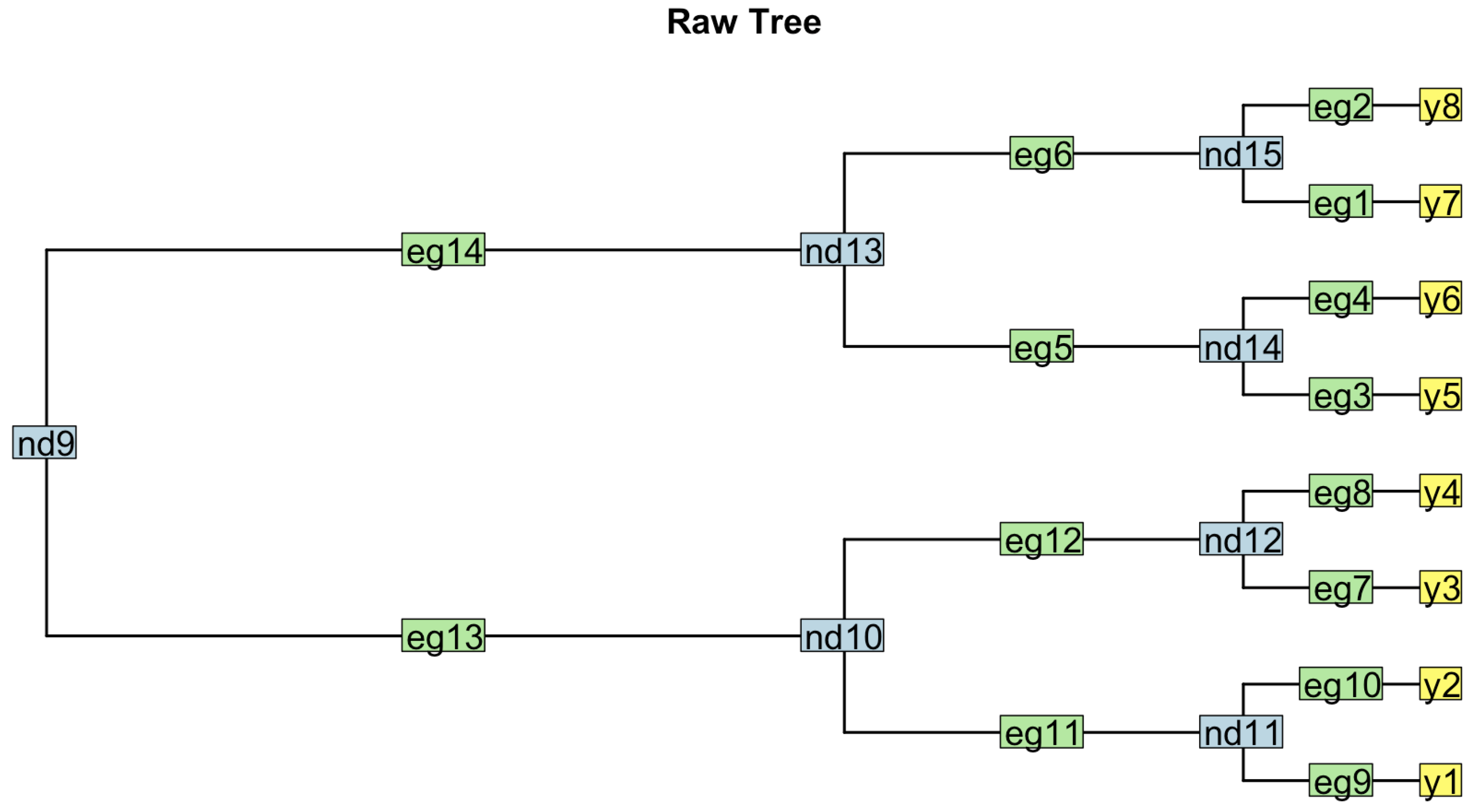
Trait values in Table 18.

Table 18.
Trait value.
Table 19.
Edge lengths obtained by tree with branch lengths using ape package [37].
Table 19.
Edge lengths obtained by tree with branch lengths using ape package [37].
Table 20.
Rate estimates from rrphylo.
Table 21.
Maximum likelihood for parameter estimates under each model.
| Model | |||||
|---|---|---|---|---|---|
| AR(1) | |||||
| AR(2) | |||||
| ARMA(1,1) | |||||
| ARMA(2,1) | |||||
| ARMA(2,2) | |||||
Table 22.
Model output. k number of parameter, AICc weight w.
| Model | k | w | Rank | ||
|---|---|---|---|---|---|
| AR1 | 2 | 1st | |||
| ARMA1 | 3 | 2nd | |||
| ARMA21 | 4 | 3th | |||
| AR2 | 3 | 4th | |||
| ARMA22 | 5 | 5th |
6.4. Trait Dataset for Empirical Analysis
For plant data and primate data, the tree files in newick format as well as the trait dataset in csv files can be accessed at https://tonyjhwueng.info/phyarmarate/dataset
References
- Pettay, J.E.; Kruuk, L.E.; Jokela, J.; Lummaa, V. Heritability and genetic constraints of life-history trait evolution in preindustrial humans. Proceedings of the National Academy of Sciences 2005, 102, 2838–2843. [Google Scholar] [CrossRef] [PubMed]
- Holstad, A.; Voje, K.L.; Opedal, Ø.H.; Bolstad, G.H.; Bourg, S.; Hansen, T.F.; Pélabon, C. Evolvability predicts macroevolution under fluctuating selection. Science 2024, 384, 688–693. [Google Scholar] [CrossRef] [PubMed]
- Scott-Phillips, T.C.; Laland, K.N.; Shuker, D.M.; Dickins, T.E.; West, S.A. The niche construction perspective: a critical appraisal. Evolution 2014, 68, 1231–1243. [Google Scholar] [CrossRef] [PubMed]
- Soons, J.; Herrel, A.; Genbrugge, A.; Aerts, P.; Podos, J.; Adriaens, D.; De Witte, Y.; Jacobs, P.; Dirckx, J. Mechanical stress, fracture risk and beak evolution in Darwin’s ground finches (Geospiza). Philosophical Transactions of the Royal Society B: Biological Sciences 2010, 365, 1093–1098. [Google Scholar] [CrossRef]
- Podos, J.; Nowicki, S. Beaks, adaptation, and vocal evolution in Darwin’s finches. Bioscience 2004, 54, 501–510. [Google Scholar] [CrossRef]
- Xiang, Y.; Huang, C.H.; Hu, Y.; Wen, J.; Li, S.; Yi, T.; Chen, H.; Xiang, J.; Ma, H. Evolution of Rosaceae fruit types based on nuclear phylogeny in the context of geological times and genome duplication. Molecular biology and evolution 2017, 34, 262–281. [Google Scholar] [CrossRef]
- Thorne, J.L.; Kishino, H.; Painter, I.S. Estimating the rate of evolution of the rate of molecular evolution. Molecular biology and evolution 1998, 15, 1647–1657. [Google Scholar] [CrossRef]
- Uyeda, J.C.; Zenil-Ferguson, R.; Pennell, M.W. Rethinking phylogenetic comparative methods. Systematic Biology 2018, 67, 1091–1109. [Google Scholar] [CrossRef]
- Garamszegi, L.Z. Modern phylogenetic comparative methods and their application in evolutionary biology: concepts and practice; Springer, 2014.
- Cornwell, W.; Nakagawa, S. Phylogenetic comparative methods. Current Biology 2017, 27, R333–R336. [Google Scholar] [CrossRef]
- OMeara, B.; Ané, C.; Sanderson, M.; Wainwright, P. Testing different rates of continuous trait evolution using likelihood. Evolution 2006, 60, 922–933. [Google Scholar]
- Adams, D.C. A method for assessing phylogenetic least squares models for shape and other high-dimensional multivariate data. Evolution 2014, 68, 2675–2688. [Google Scholar] [CrossRef] [PubMed]
- Maddison, W.P.; Midford, P.E.; Otto, S.P. Estimating a binary character’s effect on speciation and extinction. Systematic biology 2007, 56, 701–710. [Google Scholar] [CrossRef] [PubMed]
- Uyeda, J.C.; Hansen, T.F.; Arnold, S.J.; Pienaar, J. The million-year wait for macroevolutionary bursts. Proceedings of the National Academy of Sciences 2011, 108, 15908–15913. [Google Scholar] [CrossRef] [PubMed]
- Gingerich, P.D. Rates of evolution on the time scale of the evolutionary process. Microevolution rate, pattern, process 2001, 127–144. [Google Scholar]
- Felsenstein, J. Phylogeny and the comparative method. America Naturalist 1985, 125, 1–15. [Google Scholar] [CrossRef]
- Jhwueng, D.C.; Maroulas, V. Adaptive trait evolution in random environment. Journal of Applied Statistics 2016, 43, 2310–2324. [Google Scholar] [CrossRef]
- Jhwueng, D.C. Modeling rate of adaptive trait evolution using Cox–Ingersoll–Ross process: An Approximate Bayesian Computation approach. Computational Statistics & Data Analysis 2020, 145, 106924. [Google Scholar]
- Davis, C.C.; Latvis, M.; Nickrent, D.L.; Wurdack, K.J.; Baum, D.A. Floral gigantism in Rafflesiaceae. Science 2007, 315, 1812–1812. [Google Scholar] [CrossRef]
- Beaulieu, J.; Jhwueng, D.C.; Boettiger, C.; O’öMeara, B. Modeling stabilizing selection: expanding the Ornstein-Uhlenbeck model of adaptive evolution. Evolution 2012, 66, 2369–2383. [Google Scholar]
- Tsay, R.S. Analysis of financial time series; Vol. 543, John wiley & sons, 2005.
- Pham, H.T.; Yang, B.S. Estimation and forecasting of machine health condition using ARMA/GARCH model. Mechanical Systems and Signal Processing 2010, 24, 546–558. [Google Scholar] [CrossRef]
- Sakamoto, M.; Venditti, C. Phylogenetic non-independence in rates of trait evolution. Biology letters 2018, 14, 20180502. [Google Scholar] [CrossRef] [PubMed]
- Bollerslev, T. Generalized autoregressive conditional heteroskedasticity. Journal of econometrics 1986, 31, 307–327. [Google Scholar] [CrossRef]
- Engle, R. GARCH 101: The use of ARCH/GARCH models in applied econometrics. Journal of economic perspectives 2001, 15, 157–168. [Google Scholar] [CrossRef]
- Castiglione, S.; Serio, C.; Mondanaro, A.; Melchionna, M.; Carotenuto, F.; Di Febbraro, M.; Profico, A.; Tamagnini, D.; Raia, P. Ancestral state estimation with phylogenetic ridge regression. Evolutionary Biology 2020, 47, 220–232. [Google Scholar] [CrossRef]
- Castiglione, S.; Tesone, G.; Piccolo, M.; Melchionna, M.; Mondanaro, A.; Serio, C.; Di Febbraro, M.; Raia, P. A new method for testing evolutionary rate variation and shifts in phenotypic evolution. Methods in Ecology and Evolution 2018, 9, 974–983. [Google Scholar] [CrossRef]
- Song, G.; Zhu, L.; Gao, A.; Kong, L. Blockwise AICc and its consistency properties in model selection. Communications in Statistics-Theory and Methods 2021, 50, 3198–3213. [Google Scholar] [CrossRef]
- Zhang, J.; Yang, Y.; Ding, J. Information criteria for model selection. Wiley Interdisciplinary Reviews: Computational Statistics 2023, 15, e1607. [Google Scholar] [CrossRef]
- Henniges, M.C.; Johnston, E.; Pellicer, J.; Hidalgo, O.; Bennett, M.D.; Leitch, I.J. The Plant DNA C-Values Database: a one-stop shop for plant genome size data. In Plant Genomic and Cytogenetic Databases; Springer, 2023; pp. 111–122.
- Hedges, S.B.; Dudley, J.; Kumar, S. TimeTree: a public knowledge-base of divergence times among organisms. Bioinformatics 2006, 22, 2971–2972. [Google Scholar] [CrossRef]
- Sanderson, M.J. Estimating absolute rates of molecular evolution and divergence times: a penalized likelihood approach. Molecular biology and evolution 2002, 19, 101–109. [Google Scholar] [CrossRef]
- Galán-Acedo, C.; Arroyo-Rodríguez, V.; Andresen, E.; Arasa-Gisbert, R. Ecological traits of the world’s primates. Scientific Data 2019, 6, 55. [Google Scholar] [CrossRef]
- Dewey, T.; Shefferly, N.; Havens, A. Animal Diversity Web. University of Michigan Museum of Zoology 2010. [Google Scholar]
- Dyer, M.A.; Martins, R.; da Silva Filho, M.; Muniz, J.A.P.; Silveira, L.C.L.; Cepko, C.L.; Finlay, B.L. Developmental sources of conservation and variation in the evolution of the primate eye. Proceedings of the National Academy of Sciences 2009, 106, 8963–8968. [Google Scholar] [CrossRef] [PubMed]
- Andrei, N. Modern Numerical Nonlinear Optimization; Vol. 195, Springer, 2022.
- Paradis, E.; Schliep, K. ape 5.0: an environment for modern phylogenetics and evolutionary analyses in R. Bioinformatics 2019, 35, 526–528. [Google Scholar] [CrossRef] [PubMed]
Figure 1.
Trajectories of Brownian motion using two different rates (left: , right: ). The time space is set to 100. The histograms are plotted using the endpoints of the trajectories.
Figure 1.
Trajectories of Brownian motion using two different rates (left: , right: ). The time space is set to 100. The histograms are plotted using the endpoints of the trajectories.
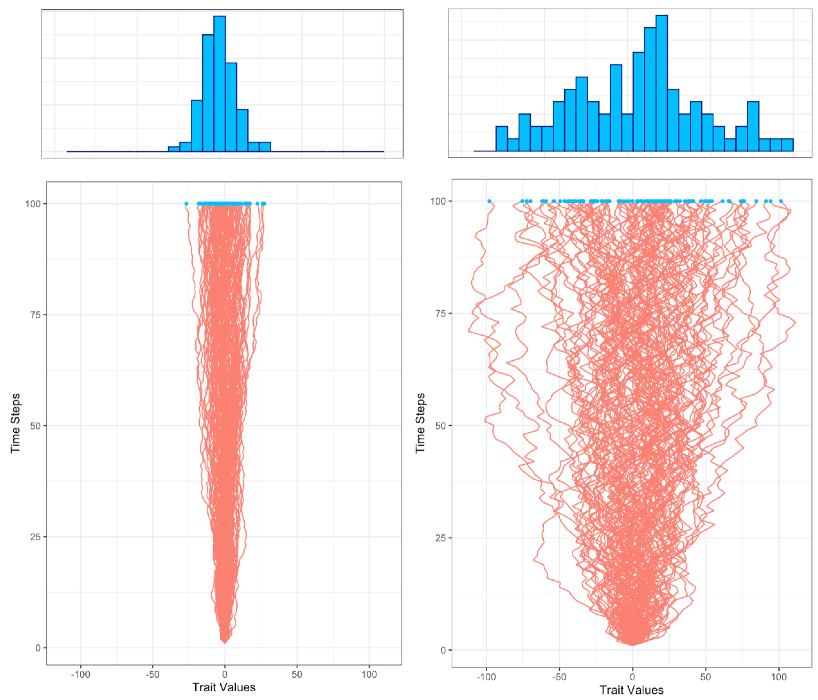
Figure 2.
Trajectories of trait evolution for 4 species along a rooted phylogenetic tree. Middle panel: four taxa rooted tree of 4 tips . Left panel: a set of four dependent trajectories along the tree using a single rate ( on all branches). Right panel: a set of four dependent trajectories along the tree using two rates ( on the blue branches, and on the red branches). is the root status denoted as a parameter of interest (analogous to ).
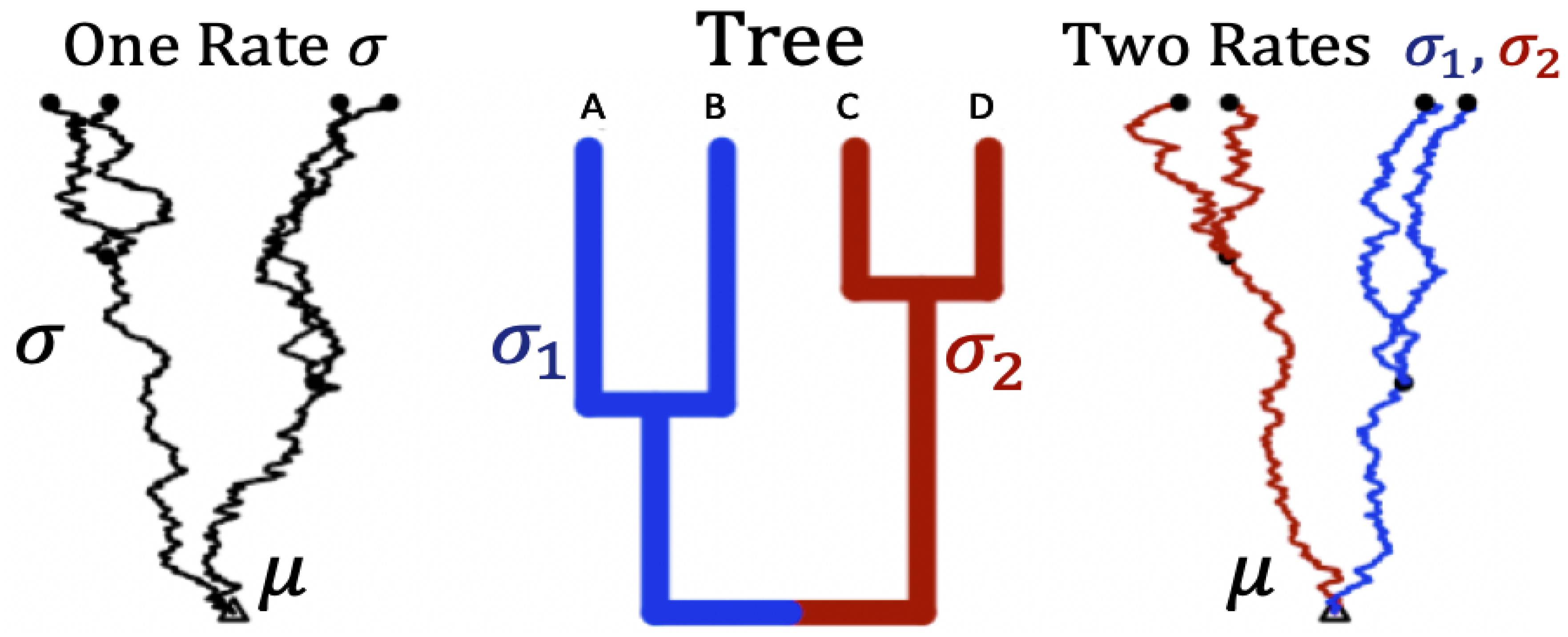
Figure 3.
A rooted phylogenetic tree of three taxa with tip nodes A, B, and C, internal nodes D and E, and root node O, where the branch lengths are , , , , and , and the rate variables are , , , , and .
Figure 3.
A rooted phylogenetic tree of three taxa with tip nodes A, B, and C, internal nodes D and E, and root node O, where the branch lengths are , , , , and , and the rate variables are , , , , and .
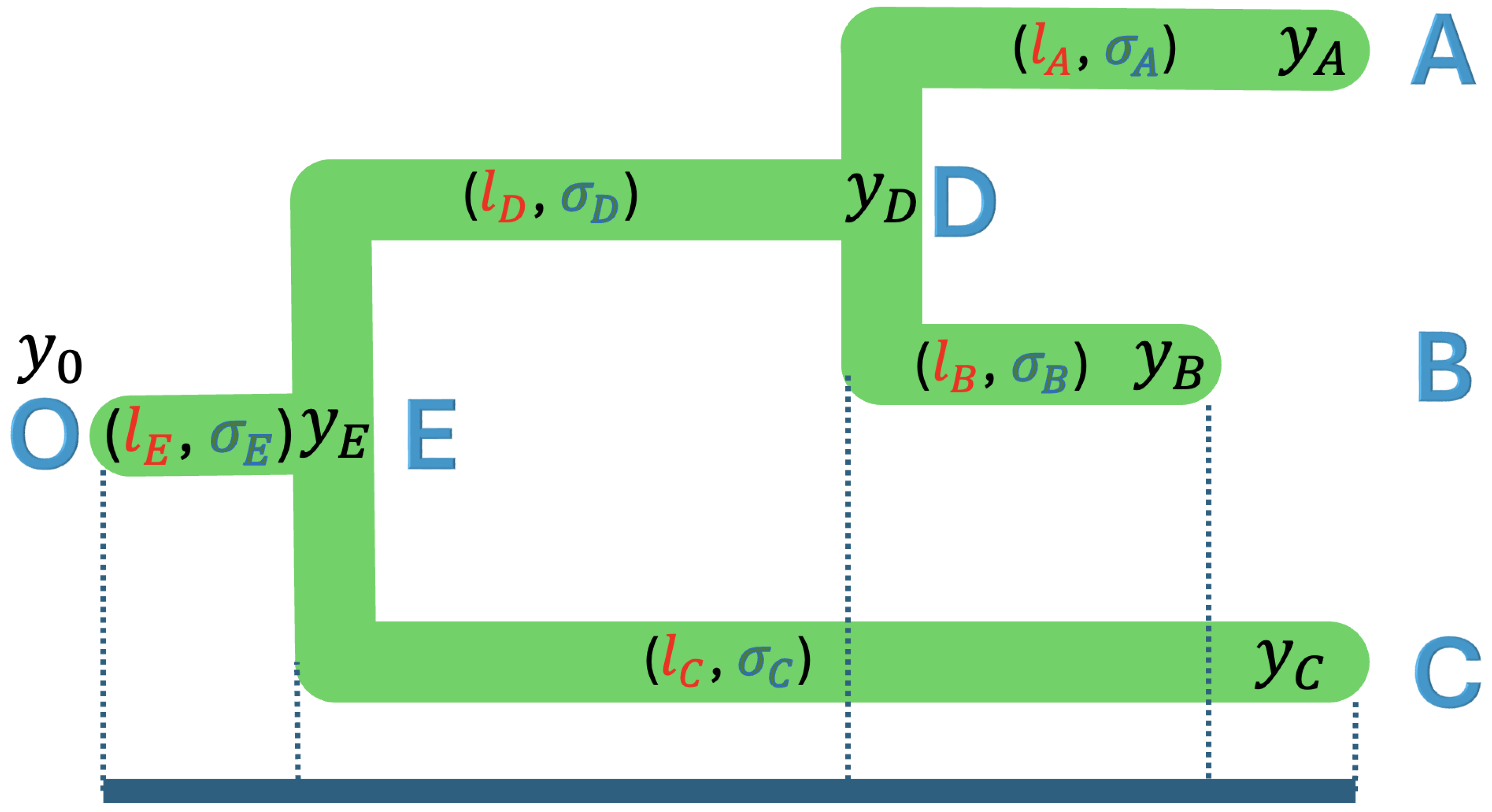
Figure 4.
The phylogenetic ARMA rate model for the rate of evolution along the tree. The root status O starts with , along the tree the error of the rate estimate. The ARMA rates are bond to the tree toplogy’s ancestral-descendant relationship. For instance, the rate at tip node A has the relationship with the ancestor node D of where while the rate at internal node D has the relationship with the ancestor node E of where .
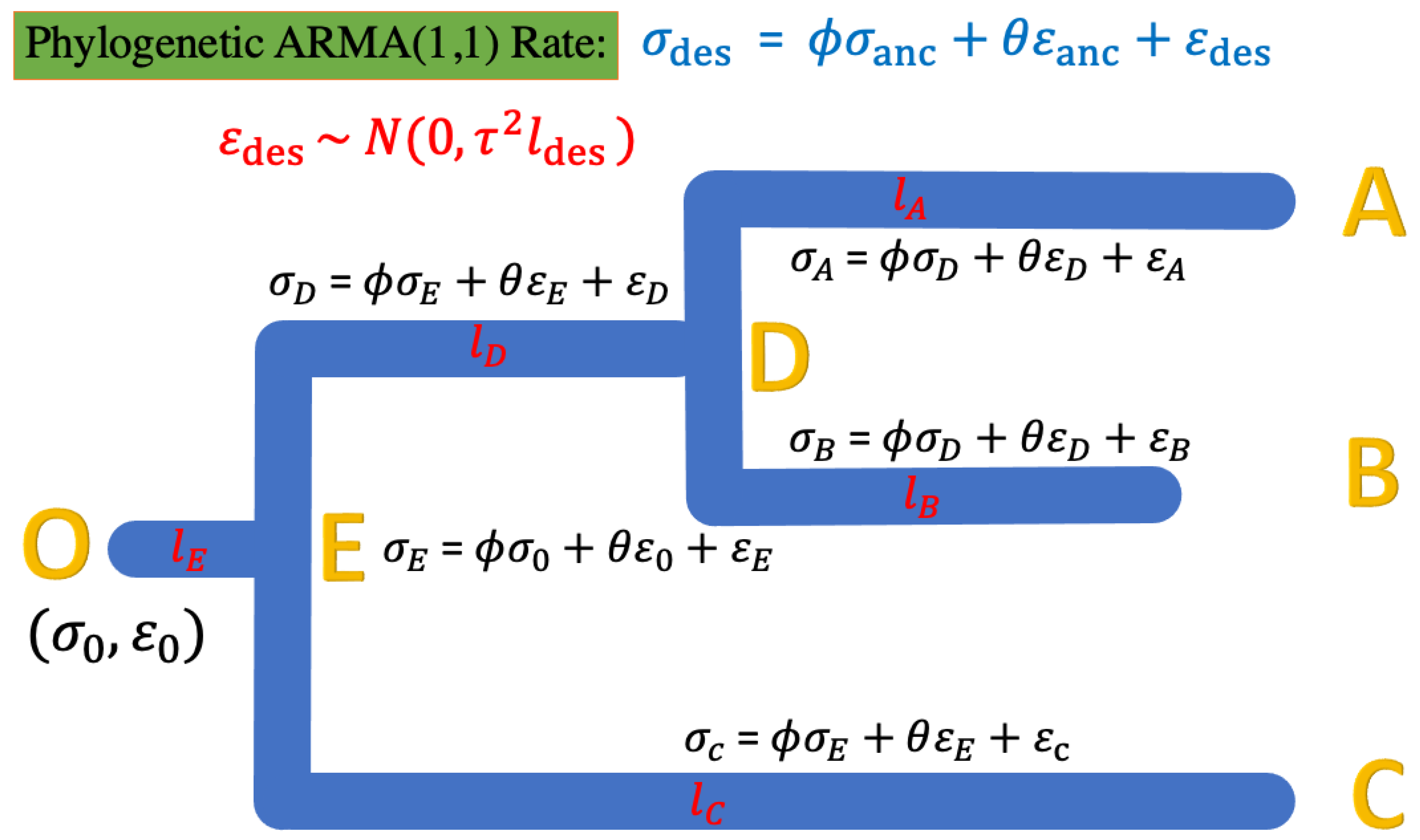
Figure 5.
Test heterogeneity rates for the trait evolution on the two sub clade of the tree. Test for two ’s () vs. one .
Figure 5.
Test heterogeneity rates for the trait evolution on the two sub clade of the tree. Test for two ’s () vs. one .
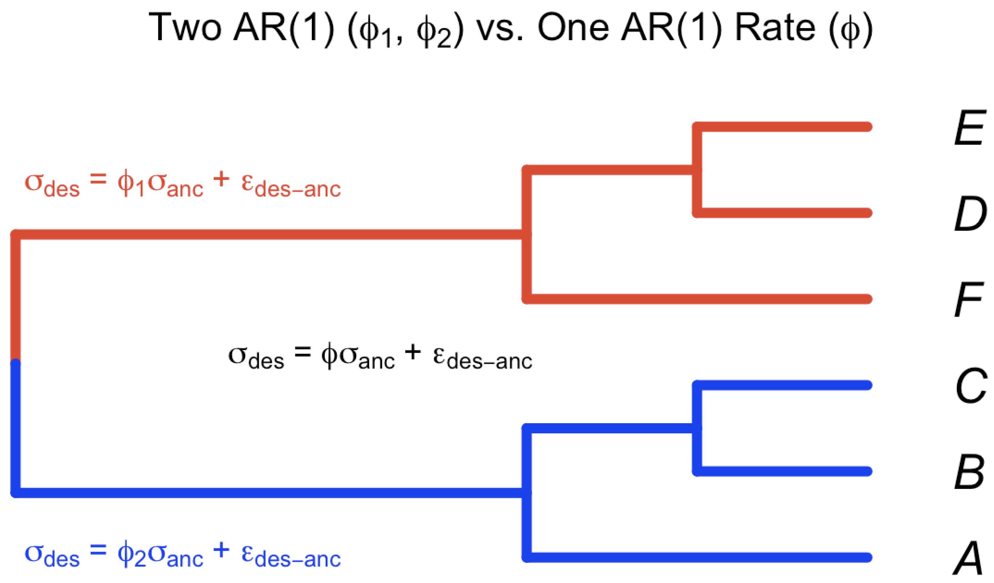
Figure 6.
Power Curve for varying Taxa levels. The horizontal axis represents an adjusted value of a parameter called , ranging from 0 to near 1. The vertical axis depicts the statistical power, indicating the probability of rejecting a null hypothesis when an alternative is true; a range from 0 suggests no detection ability, while 1 signifies certain detection. The four curves represent different Taxa counts , which could indicate distinct sample sizes or biological classifications. The horizontal lines present the type I error rate using level .
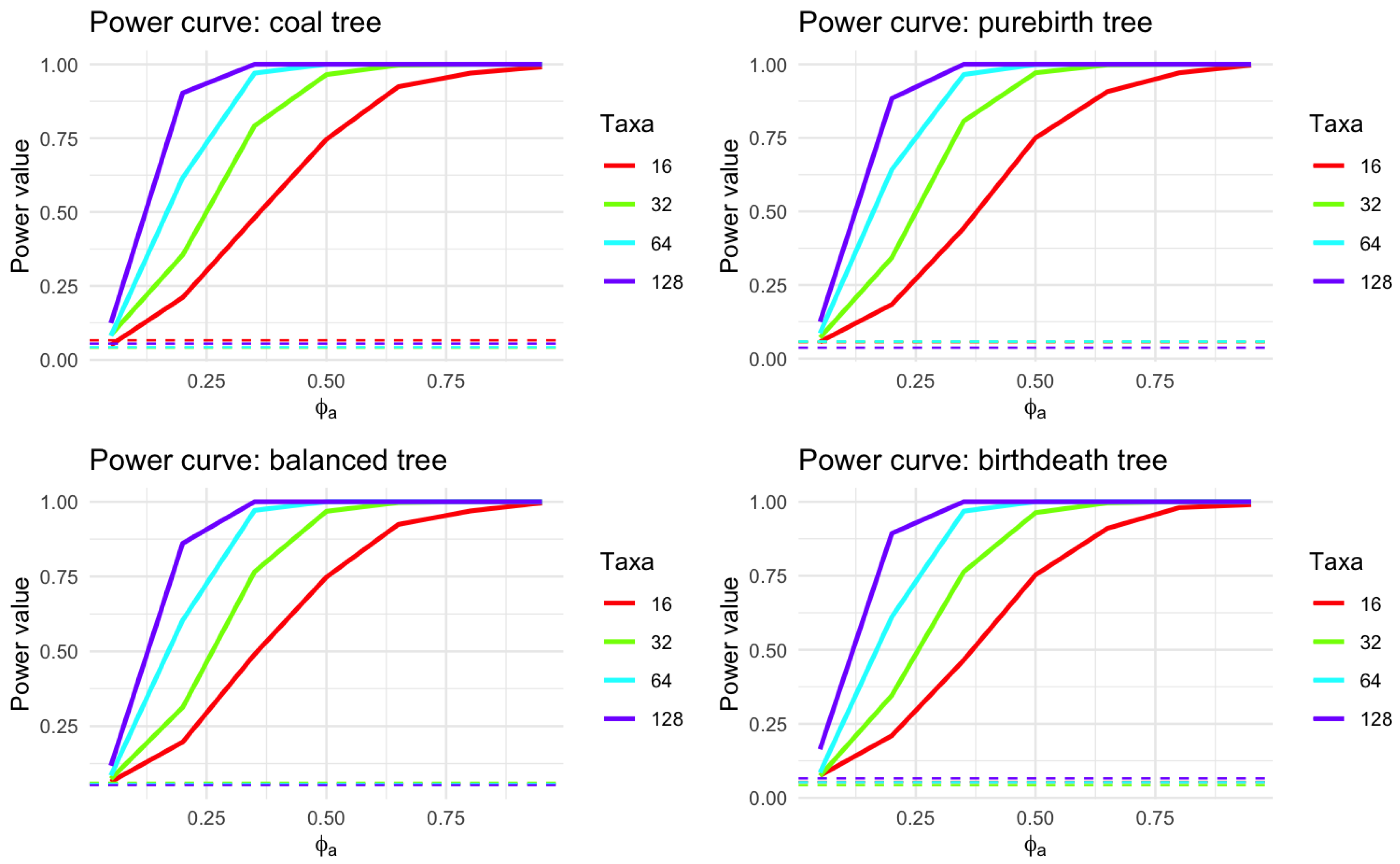
Figure 7.
Left: herbaticus tree. Right: woody specie midddle: combined herbaticus and woody species. The herbaticus and woody trees are obtained by TimeTree [31] where species names are entered and the system generate the tree in Newick format, and the combined tree is obtained by using R ape package function bind.tree with applying the molecular dating with penalized likelihood approach [32] for branch length estimation. This is done by using the R function chronopl for taking the herbaticus tree and woody tree as input.
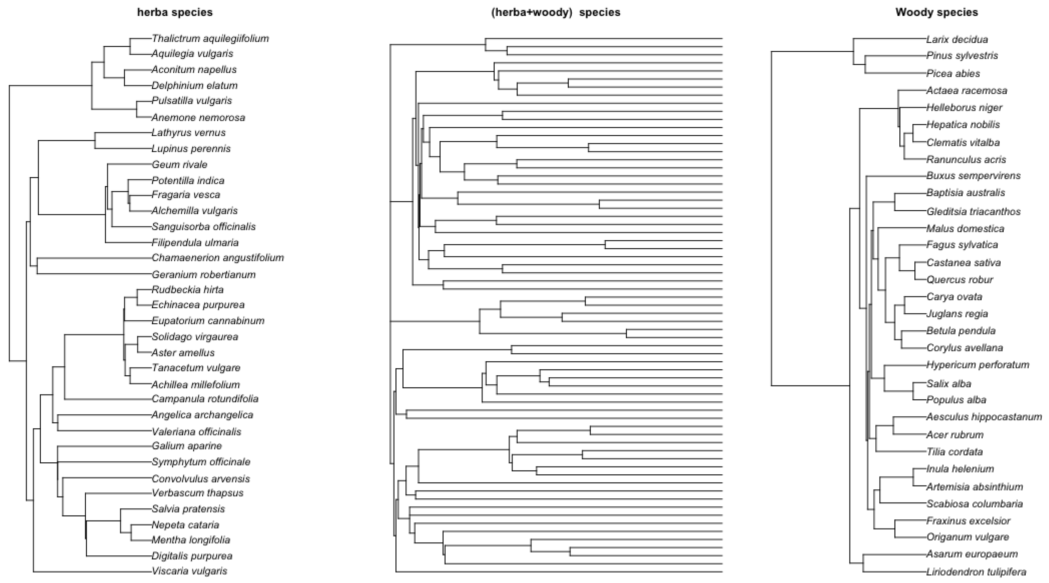
Figure 8.
Left: tree with 54 nocturnal primate. Right: tree with 28 diurnal primate. Middle: combined phylogenetic tree of 88 primate species [33,35].
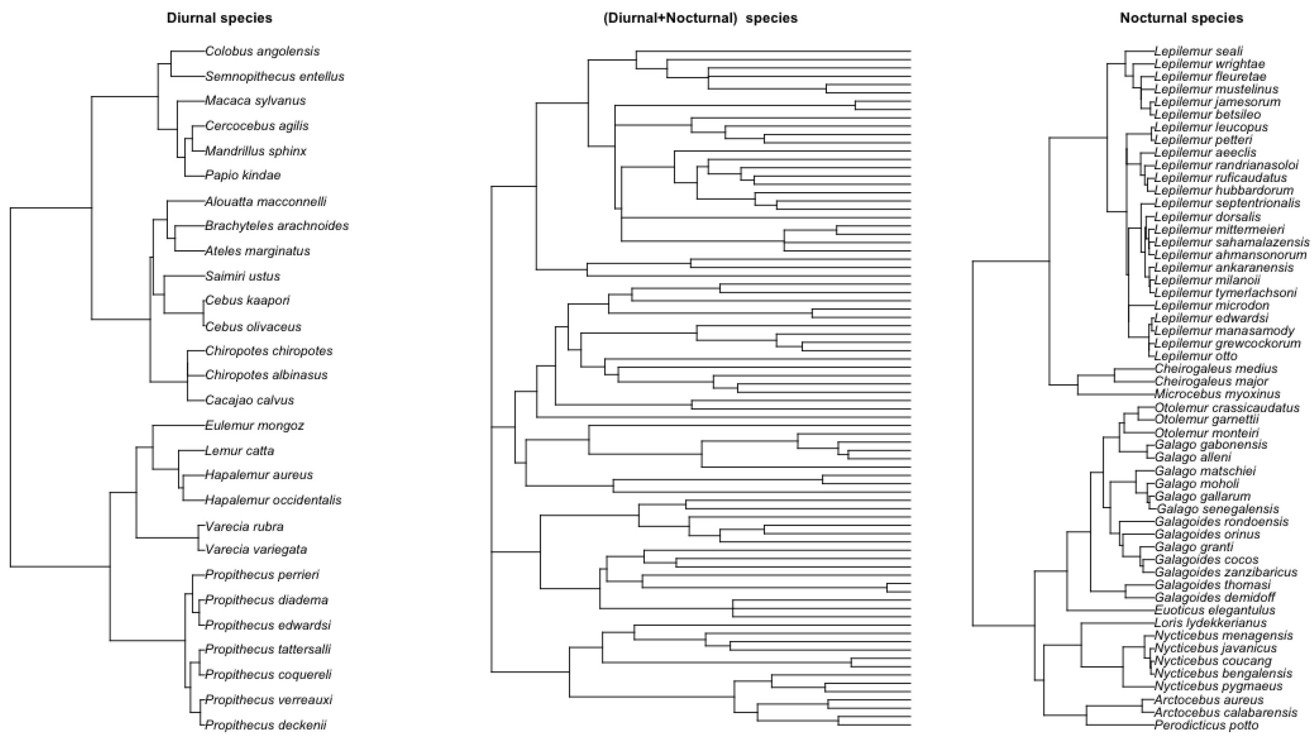
Table 1.
The type I error (T1 err) rate and the power of tree AR(1) rate on the null using 4 type of tree and 4 taxa size. The alternative are set to values , respectively. 1000 replicates are used and the significance level is set to .
Table 1.
The type I error (T1 err) rate and the power of tree AR(1) rate on the null using 4 type of tree and 4 taxa size. The alternative are set to values , respectively. 1000 replicates are used and the significance level is set to .
| Tree type | Taxa | T1 err | |||||||
|---|---|---|---|---|---|---|---|---|---|
| Balanced | 16 | 0.066 | 0.050 | 0.211 | 0.481 | 0.746 | 0.924 | 0.970 | 0.991 |
| 32 | 0.041 | 0.084 | 0.355 | 0.792 | 0.965 | 0.997 | 1.000 | 1.000 | |
| 64 | 0.043 | 0.081 | 0.616 | 0.970 | 1.000 | 1.000 | 1.000 | 1.000 | |
| 128 | 0.055 | 0.124 | 0.903 | 1.000 | 1.000 | 1.000 | 1.000 | 1.000 | |
| Pure Birth | 16 | 0.056 | 0.057 | 0.184 | 0.443 | 0.750 | 0.907 | 0.971 | 0.997 |
| 32 | 0.057 | 0.071 | 0.343 | 0.807 | 0.971 | 0.998 | 1.000 | 1.000 | |
| 64 | 0.058 | 0.086 | 0.642 | 0.965 | 0.999 | 1.000 | 1.000 | 1.000 | |
| 128 | 0.037 | 0.125 | 0.884 | 1.000 | 1.000 | 1.000 | 1.000 | 1.000 | |
| Birth Death | 16 | 0.058 | 0.064 | 0.197 | 0.490 | 0.748 | 0.924 | 0.969 | 0.996 |
| 32 | 0.061 | 0.074 | 0.313 | 0.766 | 0.968 | 0.997 | 1.000 | 1.000 | |
| 64 | 0.057 | 0.085 | 0.604 | 0.971 | 1.000 | 1.000 | 1.000 | 1.000 | |
| 128 | 0.053 | 0.118 | 0.861 | 1.000 | 1.000 | 1.000 | 1.000 | 1.000 | |
| Balanced | 16 | 0.054 | 0.075 | 0.210 | 0.465 | 0.753 | 0.910 | 0.980 | 0.990 |
| 32 | 0.043 | 0.074 | 0.346 | 0.763 | 0.963 | 0.996 | 1.000 | 1.000 | |
| 64 | 0.053 | 0.085 | 0.611 | 0.968 | 1.000 | 1.000 | 1.000 | 1.000 | |
| 128 | 0.066 | 0.164 | 0.893 | 1.000 | 1.000 | 1.000 | 1.000 | 1.000 |
Table 2.
MLE parameter estimated for the combined hebaticus (35) and woody (33) 68 species.
| AR(1) | |||||
| AR(2) | |||||
| ARMA(1,1) | |||||
| ARMA(2,1) | |||||
| ARMA(2,2) | |||||
| Weighted Estimate |
Table 3.
Model information for the combined herbaticus and woody 88 primate species.
| Model | k | w | Rank | ||
|---|---|---|---|---|---|
| AR(2) | 3 | 1st | |||
| AR(1) | 2 | 2nd | |||
| ARMA(1,1) | 3 | 3rd | |||
| ARMA(2,1) | 4 | 4th | |||
| ARMA(2,2) | 5 | 5th |
Table 4.
Herbaticus species model parameter estimates.
| AR(1) | |||||
| AR(2) | |||||
| ARMA(1,1) | |||||
| ARMA(2,1) | |||||
| ARMA(2,2) | |||||
| Weighted Estimate |
Table 5.
Herbaticus species model results.
| Model | k | w | Rank | ||
|---|---|---|---|---|---|
| AR(1) | 2 | 1st | |||
| ARMA(1,1) | 3 | 2nd | |||
| AR(2) | 3 | 4th | |||
| ARMA(2,1) | 4 | 3rd | |||
| ARMA(2,2) | 5 | 5th |
Table 6.
Woody species model parameter estimates.
| AR(1) | |||||
| AR(2) | |||||
| ARMA(1,1) | |||||
| ARMA(2,1) | |||||
| ARMA(2,2) | |||||
| Weighted Estimate |
Table 7.
Woody species model results.
| Model | k | w | Rank | ||
|---|---|---|---|---|---|
| AR(1) | 2 | 1st | |||
| ARMA(1,1) | 3 | 2nd | |||
| ARMA(2,2) | 5 | 3rd | |||
| ARMA(2,1) | 4 | 4th | |||
| AR(2) | 3 | 5th |
Table 8.
, .
| Tree case | z-val | p-val | significant ? |
|---|---|---|---|
| combined tree | N | ||
| herbaticus tree | Y | ||
| woody tree | N |
Table 9.
Testing heterogeneity rates on subclades. : , : .
| Model | _di | _no | _dino | p-val | Significant? | |
|---|---|---|---|---|---|---|
| AR(1) | Y | |||||
| AR(2) | Y | |||||
| ARMA(1,1) | Y | |||||
| ARMA(2,1) | Y | |||||
| ARMA(2,2) | Y |
Table 10.
MLE parameter estimated for the combined dirunal and nocturnal 88 primate species.
| AR(1) | |||||
| AR(2) | |||||
| ARMA(1,1) | |||||
| ARMA(2,1) | |||||
| ARMA(2,2) | |||||
| Weighted Estimate |
Table 11.
Model information for the combined dirunal and nocturnal 88 primate species.
| Model | k | w | Rank | ||
|---|---|---|---|---|---|
| ARMA(1) | 3 | 1st | |||
| ARMA(2,1) | 4 | 2nd | |||
| ARMA(2,2) | 5 | 3rd | |||
| AR(2) | 3 | 4th | |||
| AR(1) | 2 | 5th |
Table 12.
Diurnal species model parameter estimates.
| AR(1) | |||||
| AR(2) | |||||
| ARMA(1,1) | |||||
| ARMA(2,1) | |||||
| ARMA(2,2) | |||||
| Weighted Estimate |
Table 13.
Diurnal species model results.
| Model | k | w | Rank | ||
|---|---|---|---|---|---|
| AR(1) | 2 | 1st | |||
| ARMA(1,1) | 3 | 2nd | |||
| AR(2) | 3 | 3rd | |||
| ARMA(2,1) | 4 | 4th | |||
| ARMA(2,2) | 5 | 5th |
Table 14.
Nocturnal species model parameter estimates.
| AR(1) | |||||
| AR(2) | |||||
| ARMA(1,1) | |||||
| ARMA(2,1) | |||||
| ARMA(2,2) | 0.004 | ||||
| Weighted Estimate |
Table 15.
Nocturnal species model results.
| Model | k | w | Rank | ||
|---|---|---|---|---|---|
| AR(1) | 2 | 1st | |||
| AR(2) | 3 | 2nd | |||
| ARMA(1,1) | 3 | 3th | |||
| ARMA(2,1) | 4 | 4th | |||
| ARMA(2,2) | 5 | 5th |
Table 16.
, .
| Tree case | z-val | p-val | significant ? |
|---|---|---|---|
| Diurnal tree | Y | ||
| Nocturnal tree | Y | ||
| Combined tree | Y |
Table 17.
Testing Heterogeity Rates on subclade. : one , : .
| Model | _di | _no | _dino | p-val | Significant? | |
|---|---|---|---|---|---|---|
| AR(1) | Y | |||||
| AR(2) | - | Y | ||||
| ARMA(1,1) | Y | |||||
| ARMA(2,1) | Y | |||||
| ARMA(2,2) | Y |
Disclaimer/Publisher’s Note: The statements, opinions and data contained in all publications are solely those of the individual author(s) and contributor(s) and not of MDPI and/or the editor(s). MDPI and/or the editor(s) disclaim responsibility for any injury to people or property resulting from any ideas, methods, instructions or products referred to in the content. |
© 2024 by the author. Licensee MDPI, Basel, Switzerland. This article is an open access article distributed under the terms and conditions of the Creative Commons Attribution (CC BY) license (https://creativecommons.org/licenses/by/4.0/).
Copyright: This open access article is published under a Creative Commons CC BY 4.0 license, which permit the free download, distribution, and reuse, provided that the author and preprint are cited in any reuse.


