
Submitted:
25 November 2024
Posted:
27 November 2024
You are already at the latest version
Abstract
A global motivation to reduce reliance on fossil fuels and transition to cleaner, renewable energy sources propels studies of innovative technologies to harness solar energy. This paper investigates the viability of Solar Chimney Power Plants (SCPP) in a domestic context. Using a mathematical model, including thermodynamic processes within the collector, chimney and turbine generator, the power output of SCPPs is assessed across five global locations with varying annual energy requirements: Aswan Egypt, Cornwall UK, Melbourne Australia, Quito Ecuador, São Paulo Brazil. This research aims to predict plant performance under differing geometries and meteorological inputs such as ambient temperature and solar irradiance, revealing that Aswan, Quito, and São Paulo can reliably produce year-round power, while Cornwall and Melbourne may need a supplementary energy supply in the winter months. The model establishes a linear relationship between collector radius and chimney height for each region to minimize geometry whilst fulfilling annual energy requirements, demonstrating that reducing one component size increases the other to maintain the required output; for Quito, with the lowest annual energy requirement, and therefore this results in a collector radius of approximately 25m and a chimney height of approximately 70m. These geometries inform discussions of technology implementation, including the integration of an Air Source Heat Pump (ASHP) to enhance performance, though it was found that the SCPP may not meet the power demand of the ASHP in Melbourne winter. Some lifecycle factors of the Melbourne and Quito plants are considered to assess the environmental viability of the technology. It was found that material selection influences plant performance and is the greatest contributor to the carbon footprint.
Keywords:
Solar Chimney Power Plant
; design
; modelling
; scaling
; hybridization
; lifecycle
1. Introduction
The ‘dangerous climate change guardrail’ of 1.5°C global temperature rise represents a pivotal threshold, beyond which the world may reach a point of no return in the face of global warming [1]. The United Nations Paris Agreement aims to mitigate this risk by targeting a 45% reduction in emissions by 2030, with the ultimate goal of achieving net zero emissions by 2050 [2]. However, with fossil fuels currently supplying around 80% of the world's energy [3] and current projections indicating a 9% increase in emissions by 2030 compared to 2010 [4], achieving the Paris Agreement targets requires a radical shift in energy production away from fossil fuels and towards clean, renewable sources.
A Solar Chimney Power Plant (SCPP), shown in Figure 1, is a technology that utilizes well-known principles to create renewable energy from solar radiation with low carbon emissions. These are the greenhouse effect, the buoyancy effect, and the conversion of kinetic energy into electrical energy via a turbine generator.
Figure 1(a) displays the three main components of a SCPP. The collector is constructed of a transparent material, such as glass, PVC, or plastic film, that is elevated above the ground and open around the perimeter. The collector uses the greenhouse effect to heat the ground below using both direct and diffuse solar radiation, which, combined with the buoyancy effect and an open perimeter, creates a solar induced convective airflow that is driven towards the centre of the collector. Here, a turbine captures the kinetic energy before the air rises up the chimney and returns to the atmosphere, as shown in Figure 1b. The air continuously moves through the system, driven by the pressure difference between the air outside and inside the SCPP. The numbered locations in Figure 1(b) will be referenced throughout the report as subscripts following the corresponding parameters.
Although large-scale SCPP’s have been widely studied, research on small-scale SCPPs and their domestic application remains limited. The motivation behind this report is to investigate the technical, practical, and environmental viability of the domestic application of a SCPP in various locations around the globe, with the aim to forecast system performance considering dimensional and meteorological parameters.
The main objectives of this report are:
- Devise a mathematical model to predict the performance of solar chimney systems in different locations with varying dimensions.
- Compare and analyse results of the systems in different locations and for different energy requirements.
- Discuss the feasibility and practical implementation of the domestic application in different locations.
A Python-based mathematical model was developed to simulate the thermodynamic processes outlined in Section 3.3.2. This model was validated using previous experimental data. Hourly meteorological data spanning a year was then fed into the model for five distinct global locations to compute the hourly power output over the course of the year.
Varying system dimensions were modelled to understand the impact on the power output. This allowed for an examination of the relationship between required energy generation and minimum system size, considering location-specific meteorological parameters. The results obtained informed a discussion on the feasibility, practicality, and environmental impact of implementing SCPP technology in diverse geographical locations, providing insights for further discussions on its application.
2. A Review of the Solar Chimney Power Plant (SCPP)
The concept of using rising hot air in a chimney to propel a turbine was first presented as a ‘smoke jack’ by Leonardo da Vinci around 1480 [5]. In 1903, Isidoro Cabanyes introduced an early form of a SCPP, outlining a ‘projecto de motor solar’ or ‘solar engine project’ featuring a collector that heats air, connected to a building with a chimney. In this setup, the heated air flows through the chimney and rotates a fan, thereby generating electricity [6]. The first SCPP prototype was constructed in Manzanares, Spain by engineering firm Schlaich & Partners in 1982 [7], as seen in Figure 2.
The Manzanares prototype was constructed with a thick collector cover made from various plastic films and glass, a reinforced concrete chimney, a blackened bitumen collector floor and a vertical axis turbine with four blades, designed for a peak power output of 50kW [9]. Some key dimensional parameters are listed in Table 1 alongside operating parameters from 2nd September 1982 at midday.
The Manzanares pilot plant was in operation for 15,000 hours from 1982, and between 1986-1989, it ran for an average of 8.9 hours a day with 95% reliability. The prototype was constructed with the purpose of performing tests and experiments in order to design larger plants with the potential of producing 200MW of power [8]. Although the Spanish prototype produced a large dataset, it is still one of the only large-scale plants that has ever been constructed, resulting in a scarcity of validation points for subsequent studies.
There were plans for construction of a large SCPP in Mildura, Australia capable of generating 200MW. With a chimney constructed from cement and steel at a height of 1km and a collector diameter of 10km, this plant came with an expected cost of AU$1.67 billion [10], making it difficult to secure funding and resulting in the eventual rejection of the plans [11].
Ghalamchi et al. [12] conducted a study to obtain experimental results on varying geometric dimensions on a pilot SCPP with a collector diameter and chimney height of 3m. They concluded that reducing the collector inlet height has a positive impact on the performance of the chimney. Lal et al. [13] built a small SCPP in Kota, India with a collector diameter of 12m and chimney height of 8m producing around 5W of electrical power at an irradiance of 820W/m2. These results informed the development of a computational model to estimate the optimum location for the turbine at a height of 0.25 – 1m inside the chimney tower. A small SCPP was constructed in Aswan, Egypt by Mekhail et al. [14] measuring 6m in both collector diameter and chimney height with a recorded maximum power of 0.85W for an irradiance of 1000W/m2 . This study aimed to expand on the mathematical model reported by Koonsrisuk et al. [15], in order to predict the performance of a larger plant. In Texas, a SCPP was constructed with a variable chimney height from 0.203 – 7.52m by Raney et al. [16] to investigate the necessary size for a 35W output. They concluded from their study that this would require a Hch of 15m and rcoll of 60m, stating that the characteristic equations of the flow still apply to the small scale SCPP’s.
Haaf et al. [9] first developed an analytical model to predict the performance of the Manzanares plant. They reported that if the collector radius is increased, output is also increased; however, this results in reduced efficiency. Also, increasing the chimney height increases the efficiency of the SCPP. They also reported that the momentary efficiency should not be a design requirement, and the most important design factor should account for the average power output over long periods of time. Zhou et al. [17] used a theoretical model to study the effect of chimney height and concluded that the optimum chimney height for the Manzanares plant is 615m for a peak power output of 102.2kW. Cuce et al. [18] developed a computational fluid dynamics model to investigate the effect of altering geometry on a variety of parameters. They found that mass flow rate is a key parameter on system performance and is equal to 1122.1kg/s for the Manzanares plant with an irradiance of 1000W/m2.
A mathematical model was used by Koonsrisuk et al. [15] [19] to investigate the power production of a SCPP based on the geometry. They reported that the power generated per unit of land area is proportional to the length scale of the power plant, although this cannot increase indefinitely as other losses are introduced as the system gets larger, altering the simple model. Setareh [20] developed a comprehensive mathematical model, similar to the one used in this report. They proposed that the collector heat loss coefficient is not a fixed value but instead is calculated from a variety of dimensional, environmental, and material parameters. They included the effect of ambient wind in the model and stated that increasing wind velocity has a “remarkable positive effect” on the performance of the plant.
Haaf et al. [9] reported on the effect of environmental factors such as the local climate, where a lower ambient temperature leads to an increased efficiency of the system. Also, the collector characteristics, such as floor solar absorption and cover transmissivity, determine how much of the solar radiation is converted to thermal energy. Haaf et al. [7] found that dust deposits on the collector cover influenced the transmissivity, but for smooth materials such as polyester, the dust adhesion was extremely low and, after rain showers, only decreased the transmission value by up to 2%. Kreetz [21] proposed using black plastic pipes filled with water under the collector as a form of thermal storage, with his numerical model indicating that this would make 24-hour power production possible. Das et al. [22] reports in depth on a variety of materials and their properties that can be used in the construction of the SCPP components and the corresponding effect on the performance of the plant.
There are several methods reported to calculate the power output of the SCPP system, as outlined in Table 2, resulting in some discrepancies between model results.
Haaf et al. [9] used this method to design the Manzanares pilot plant with a maximum power capacity of 50kW. However, the actual maximum output of the plant was 36kW [7], and this difference was attributed to losses over the turbine.
Aside from the pilot plant in Manzanares, all of the subsequent experimental studies have been limited to laboratory sized plants, with Ref. [22] reporting that Hch values are limited to 0.2 – 12m. This gives a basic understanding of the real flow behavior to inform mathematical and numerical studies. On the other hand, the wide range of numerical and analytical studies all focus on large-scale commercial plant sizes, with Ref. [22] reporting that Hch values studied are between 123 – 1500m, and therefore research into domestic SCPP’s is very limited. The main finding from all studies indicates that an increase in the size of the system increases the power output.
For the purpose of this paper, the effect of ambient wind is neglected for simplicity and the collector loss coefficient is a fixed value, establishing uniformity throughout the models. The power output chosen for use in this report is consistent with that of Mekhail et al. and Setareh due to the smaller number of input parameters resulting in a simpler model and ensuring consistency for each location.
3. Methodology
3.1. Location
Initially, 10 to 15 locations were considered across all continents and eventually condensed down to 5 for the purpose of this paper. The locations shown in Figure 3 were selected to represent a variety of latitude, longitude, altitude, and terrain. Two locations are each in the northern and southern hemispheres and one location is on the equator.
Previous studies have investigated the potential for SCPP’s in Aswan [14], Victoria, Australia [11], and Brazil [23], supporting the decision to report on these locations. No studies have been conducted on SCPP’s in the UK, so the southwest region was selected due to having the highest GHI, and therefore being the most feasible, across twenty locations in 2019 according to Ref. [24]. Quito was selected for its equatorial position as well as its high altitude. As altitude increases, the atmospheric pressure decreases, highlighting the effect of atmospheric pressure and air buoyancy on the output of the Quito plant.
Another selection criterion was the variation in average household energy use across the different locations, presenting an opportunity for conducting location-specific studies to determine the minimum dimensions necessary for each area. Table 3 outlines the average yearly domestic power consumption for each location.
3.2. Meteorological Data
An online database was used to obtain hourly data over the years 2007 and 2023 in a CSV format for the following parameters: air temperature, global horizontal irradiance, and surface pressure [30]. The 2023 data was averaged over 4-weekly intervals to produce the plots in Figure 4 and shows a similar trend for average temperature and irradiance at each location. The seasonal variation for each location is observed, where the peaks for each location reflect the summer according to the hemisphere. Quito shows a steady year-round irradiance and temperature due to its equatorial location.
3.3. Modelling
When devising the model, some assumptions were made in order to simplify the problem and ensure a consistent approach throughout. The main assumptions are outlined below:
- Air acts as an ideal gas, allowing for the application of the Ideal Gas Law (IGL).
- Air has the properties listed in Table 4.
- One-dimensional, steady-state airflow in order to simplify the continuity, energy, and momentum equations.
- Only Global Horizontal Irradiance (GHI) is considered in the model as it is the sum of the direct and diffuse irradiance received on a horizontal surface.
The following analysis closely follows the procedure set out in Refs. [14], [15], [19] and [20]. The pressure difference in the collector is calculated according to Equation (1), derived from the continuity, momentum, and energy equations for the flow in the collector assuming a low Mach flow [14] [15] [19] [20].
Ref. [20] proposed that the temperature change in the collector is also derived from the
continuity, momentum, and energy equations with the assumption of a low Mach flow:
The IGL, equation 3, is used to calculate the air density at each chimney component.
The mass flow rate is calculated using Equation (4) and is assumed to be constant throughout.
The solar heat flux absorbed by the collector floor can be calculated using Equation (6) [20].
Equation (7) is the dry adiabatic lapse rate equation, which shows the temperature decrease with an increase in height, assuming the air is unsaturated [19].
The pressure at the chimney exit is calculated using the hydrostatic equation and Equations 3 and 7 [19]:
Equation (7) can be applied to the temperature change in the chimney tower to calculate the temperature at the chimney exit in Equation (9) [19].
The pressure at the chimney base is calculated by combining Equations 3 and 9 with the hydrostatic equation and then integrating the derived equation to obtain Equation (10) [20].
Draught equation is used to calculate the pressure difference across the turbine by calculating the other pressure losses in the system and subtracting them from the total pressure potential [20] [33].
The total pressure potential is regarded as the pressure difference between the column of cold air outside the chimney tower and the column of hot air inside, as calculated in Equation (12) [14] [19] [20].
The inlet pressure drops, and pressure drop due to kinematic energy loss of the outlet flow are computed using equation 13 [20].
where K, the pressure loss coefficient, is equal to 1, 0.25 and 1 in Δpcoll,i, Δpturb,i, and Δpdyn respectively [20]. The frictional pressure drop in the collector and chimney is estimated from the Darcy-Weisbach equation, show in Equation (14) [20].
Darcy’s friction factor is calculated as shown in Equation (15) [34] [33].
where the wall surface roughness of the glass collector and concrete chimney are
considered to be equal to zero and 0.002m respectively [33]. The Reynold’s number is calculated using Equation (16).
The remperature change across the turbine is calculated using Equation (17), following the first law of thermodynamics [20].
where the power output is a product of the turbine efficiency, volume flow rate and
The model was computed using Python following the procedure developed in the flowchart shown in Figure 5. As mass flow rate is a key performance parameter [18], the model accounts for this by iterating for , a variation on the models proposed in previous studies. This model has the capacity to compute hourly data points over a year-long period, ensuring that the outcome data retains this level of granularity. This approach provides a more accurate representation of the output compared to relying on computed averages as input parameters.
Validation of the model was carried out using the dimensions and parameters of the Manzanares pilot plant, as listed in Table 1. These results were compared to the measured experimental outputs at the Manzanares plant on 2nd September 1982 at midday and the results are shown in Table 5 [7]. The theoretical estimates closely match the experimental observations, with errors consistently under 6% for power putput of the plant, validating the reliability of the model to provide consistent results at this level of model fidelity. It can be seen that the model slightly overestimates the power output, likely as a result of the assumption of fixed loss coefficients and the exclusion of any electrical system inefficiencies.
In addition, a basic sensitivity study was performed using the data from Table 1 to determine the effect on the model output when varying the input parameters. The results can be seen in Figure 6. The study highlights a negative correlation between ambient temperature and the power output of the system and conversely, the power output increases with increasing solar irradiance, consistent with findings from Refs. [8] [9]. An important practical note on this relationship is that ambient temperature tends to increase alongside rising solar irradiance, as will be shown later in Figure 7(b), using the Melbourne meteorological data from 29th December 2023. Therefore, ambient temperature and irradiance will have a lower limit on the performance of the plant, beyond which the air under the collector will not produce a convective air flow and the plant will not operate.
4. Results Analysis
4.1. Power Output
Initially, the power outputs of each location were computed using the Manzanares plant dimensions in order to compare their performances. The highest output days in 2023 are shown in Figure 7a), alongside the irradiance and temperature plot for the highest output day in Melbourne in Figure 7b). It’s evident from Figure 7 that the daily power production closely following the irradiance level throughout the day.
The peak data for each location is listed in Table 6. For these dates, the ambient temperature and irradiance of Melbourne and Quito are very similar, however the power output in Melbourne is higher than Quito. This difference must be as a result of the lower ambient pressure in Quito due to the altitude of the city, suggesting that the performance of a SCPP decreases as altitude increases.
Figure 7a) illustrates that there is a small variation in the annual peak power output in every location, however when considering the annual power output in Figure 8, there is a large variation by location. The plot in Figure 8b) closely resembles the irradiance plot in Figure 4b), suggesting that the irradiance has a dominating effect on the output of the SCPP, and that output is proportional to irradiance. Figure 8 indicates a decline in the average power output in the winter months in Melbourne and Cornwall. Particularly Cornwall, where the output approaches zero at the beginning and end of the year, indicating that this technology may not provide year-round power in regions with low levels of irradiance.
The annual energy production by location is compared in Table 7 for the years 2007 and 2023. It can be seen that energy production in 4 out of 5 locations increases from 2007 to 2023, this is likely to be as a result of fluctuating annual irradiance.
4.2. Dimensional Study
Using the Manzanares plant parameters in Table 1, the effect of varying the dimension of each individual component was investigated with the other geometries remaining fixed. The findings for 2023 Aswan meteorological data are displayed in Figure 9. Figure 9a) indicates that there is a minimum collector radius and chimney height in order for the plant to operate, however changing the collector height and chimney radius has little impact on the performance on the system after this point. Conversely, with an increase in collector radius and chimney height, the power output increases. Figure 9b) suggests that on a small scale, the scale factor for each component is approximately equal when considering the Manzanares plant dimensions and the domestic energy demand.
The relationship between the ratios of chimney height and collector radius were considered for the Manzanares geometry by first keeping the collector radius constant and running the model with the chimney height as a varying ratio of the collector radius. Secondly, it was run with a constant chimney height and the collector radius as a varying ratio of the chimney height. For the Manzanares plant, the ratio Hch to rcoll is equal to 1.595 and the ratio of rcoll to Hch is equal to 0.627. The outcome is displayed in Figure 10, indicating that for both cases, the performance of the plant is proportional to an increase in the ratio. However, according to Figure 10b), enlarging the collector radius to exceed the chimney height increases the capacity of the plant significantly more than having the chimney height larger than the collector radius. When considering the applicability of this relationship to a domestic scenario, a reduction in the floor area occupied by the system may be preferred.
The Manzanares pilot plant dimensions were scaled down for each location to observe the effect on the annual energy production, as illustrated in Figure 11, demonstrating a clear relationship between increasing energy production with an increase in the scale factor of the plant. Figure 11b) was used to initially estimate the minimum scale factor of the Manzanares plant dimensions for each location, and this value was iterated through the model to find the minimum scale factor for the annual energy requirement, as shown in Table 8. While identifying this scale factor serves as a good initial step in determining the minimum geometries, it overlooks the optimzation of design and geometries for maximising the power output. Instead, it uses the same design and component ratios as the Manzanares pilot plant.
The scale factors from Table 8 were used to update and fix the chimney radius and collector height. The model was iterated around the chimney heights and collector radii to determine a linear relationship between the two parameters to fulfil the annual energy requirement. The results are displayed in Figure 12 alongside the least squares regression model for each location for 2007 and 2023. It is visible from the regression models that minimising one major plant dimension will lead to an increase in another plant dimension, and therefore there is not a single set of optimum geometries. Accordingly, the regression model for each location can be used in practice to determine the chimney height appropriate for a collector radius corresponding to the ground area that is available for construction.
The correlation coefficient for each regression line was calculated in Table 9, indicating a strong negative correlation for each location, and therefore imparting confidence in the regression fit.
The collector radius was calculated for a 70m chimney height for each location using the 2023 regression models. A comparison of the SCPP sizes can be seen in Figure 13. The magnitude of the size of the plant reflects the scale of the annual energy requirement by location, suggesting that the most dominating factor of plant size is the energy requirement of the region in which it is located, rather than meteorological factors. The annual energy requirement of Cornwall is only 100kWh more than Aswan, however the radius of the Aswan plant is 60% of the Cornwall plant due to the higher irradiance levels in Aswan, proposing that irradiance is the second biggest factor attributing to plant dimensions.
Using these dimensions, the plots in Figure 14 were produced to observe the plant performance in 2023. Evidently, the production in Aswan, São Paulo and Quito is steady year-round due to the consistent irradiance levels throughout all of the seasons, indicating that the technology could produce a reliable energy supply throughout the year. In contrast, the plants in Melbourne and Cornwall have a much higher peak output during the summer months due to their size. During the winter months the output drops significantly, evidencing the potential need for a supplementary energy supply or suitable energy storage to ensure the energy demand can be met during these periods. This is especially pertinent in Cornwall where the power production falls to nearly zero from November to February.
Taking a chimney height of 70m and using the regression models, the percentage change in the dimension of the radius between 2007 and 2023 is shown in Table 10. Assuming a steady change over the time period, the percentage change per year was calculated in order to forecast how the plant may perform in the future.
The results indicate that the performance of plants constructed in Quito, Aswan and São Paulo will increase annually. Whereas the performance of plants constructed in Cornwall and Melbourne would decrease annually, suggesting the need for constructing the plants with a larger collector radius to ensure viability in the future. However, as this change was only measured over two years, this would need to be tested over a continuous period to better determine the trend over time.
Although Figure 13 displays one combination of the minimum required dimensions, an observation regarding practicality of installation and maintenance of the SCPP shows that the roof height is too small for convenient access to the turbine. However, as illustrated in Figure 9, increasing the roof height does not change the annual energy production, hence for an applied system, the roof should be at least 1 metre in height.
The slenderness ratio is the ratio of the length of the chimney to the radius. Ref. [35] reports that chimneys with a slenderness ratio of up to 11.6 satisfy the permissible tensile stress for winds between 30-50m/s, meaning that chimneys with a 70m height require a radius of at least 6m in order to comply with this ratio. Even for the largest plant in Melbourne, this would mean the chimney radius will need to be more than doubled.
5. Hybridization and Lifecycle Analyses
5.1. Hybrid Options and Selection
There are many options for the extension of this SCPP model in order to make the system more effective, as reported in Ref. [36]. Five options were considered as follows: here:
- Photovoltaic (PV) panels – Located under the collector cover. Crystalline silicon PV panels become 0.2 – 0.5% less efficient for each 1°C rise in temperature. The convective air flow through the SCPP would maintain a lower surface temperature of the PV panels and therefore increase the efficiency. However, the heat absorbed by the PV panels would alter the collector properties and consequently reduce the power output of the SCPP [37].
- Air Source Heat Pump (ASHP) – Located between points 3 and 4 in the chimney tower. ASHPs are used to provide a more sustainable option for heating buildings by absorbing heat from the outside air and transferring it to an indoor space.
- Electricity storage – As an SCPP does not constantly generate power, energy storage such as large batteries could be incorporated into the design to harness the available energy. This would introduce more inefficiencies in the system; however, it could help to minimise the size of the plant to ensure the annual energy demand can be met.
- Thermal storage – As discussed in Ref. [21], this would include the use of a material to absorb some of the solar energy to be slowly released throughout the night or other periods where the plant would otherwise be inactive to allow for constant power generation. This would however decrease the peak power output as the convection induced airflow during sunlight hours would be reduced.
A Multi Criteria Decision Analysis (MCDA) was conducted to determine which option to study in more detail, as shown in Table 11. To test the sensitivity of this decision analysis, the MCDA matrix was performed with equal criteria weightings as well as those initally determined, and the outcome was unchanged. Therefore, the technology selected for further investigation was ASHP.
5.2. Analysis of a SCPP/ASHP Hybrid Plant
ASHPs operate via a reversed Carnot cycle, where a refrigerant is passed through the following components:
- Compressor - isentropic compression requiring work input.
- Condenser – isobaric heat rejection to maintain domestic temperature.
- Expansion valve – throttling.
- Evaporator – isobaric heat absorption from hot chimney air.
An ASHP could be incorporated into the SCPP system with the evaporator located between points 3 and 4 in the chimney (see Figure 1b). In order to assess the benefit of this hybrid option, the work input to the compressor must be calculated, as shown in Equation (20). Taking two winter days in Melbourne as an example, this can be calculated using the parameters in Table 12, some of which have been generated by the model.
First, the rate of heat transfer to the heated space (QH) can be calculated using Equation (19) by making some assumptions:
- The desired room temperature is 20°C and it takes 30 minutes (1800 seconds) to reach this temperature from ambient when the heating is turned on.
- The average size of a one-storey Melbourne house is 593m3 [38].
- The density of air is 1.3kg/m3, making the mass of the air inside the house equal to 770kg [39].
The Coefficient of Performance (COP) is the ratio of the useful heat transfer to the work input and is used as a measure of efficiency of the heat pump. Currently, the best ASHP’s on the market offer a maximum COP of around 5 [40]. Using this value and Equation (19), the required work input to the ASHP can be calculated from Equation (20).
Using Equations 20 and 21, the rate of heat transfer from the hot chimney air (QL) can also be calculated, and from Equation (19), the additional temperature change of the chimney air (ΔT34) can be deduced.
The outcome of these calculations can be seen in Table 13, and when comparing this with Table 12, it can be observed that the work input required to the compressor is greater than the power output on 17/08/23. However, on 07/07/23, as the solar irradiance and ambient temperature are greater, there is an increase in the power output of the SCPP and a decrease in QH, therefore suggesting there are minimum temperatures and irradiance levels for viability of the technology.
This simple process could be included as a model extension to determine the periods of viability for this hybrid option at all locations. It would be integrated in to the second iterative process in Figure 5, where Equation (9) would become:
Although this technology may be plausible, it would decrease the power available for alternative uses so it may be necessary to increase the size of the SCPP to produce sufficient power for domestic use as well as the ASHP. Hybridising the SCPP also introduces logistical complexities, such as the installation of an electrical system that is capable of powering the ASHP directly from the SCPP turbine generator.
5.3. Lifecycle Considerations
When considering the viability of a renewable energy system, both the direct and indirect environmental impact must be assessed to ensure a net positive impact. For the purpose of this report, the carbon footprint throughout the life cycle of the SCPP for two locations were evaluated. Quito and Melbourne were selected to represent the extremes in the annual energy consumption for the locations studied in this report. Correspondingly, they also reflect the range of SCPP sizes, with Quito the smallest and Melbourne the largest. The availability of materials used in construction of the largest components of the SCPP were considered, as outlined in Table 14, in order to reduce emissions associated with transportation. Copper and graphite were included as location specific materials due to their local sourcing through mining of the materials.
The properties of the collector materials are defined in Table 15. An increased transmissivity and absorptivity of the material will lead to a greater power output of the plant, as evidenced in Figure 6. Therefore, the material properties should be an important consideration to ensure a reduced size and increased power density and therefore reduced environmental impact.
Based on the information in Table 14 and Table 15, a basic EcoAudit using the Ashby method was conducted on the following materials, using the dimensions displayed in Figure 13 [50]:
- Quito – PVC collector cover, soil collector floor and concrete chimney.
- Melbourne – Glass collector cover, bitumen collector floor and concrete chimney.
These materials were selected for a combination of maximised thermo-physical properties alongside local availability and minimised CO2 footprint. The results can be seen in Figure 15.
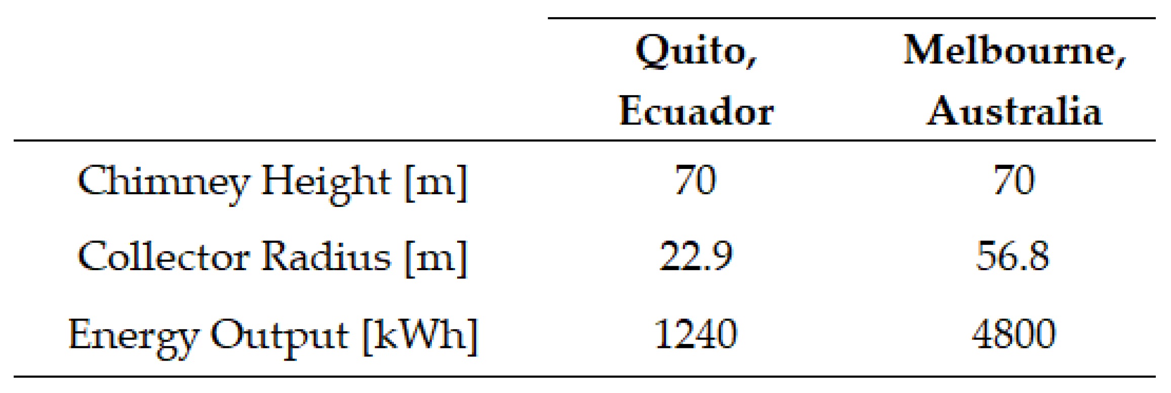
Based on a 50-year service life [53], the equivalent annual environmental burden from the construction and disposal of a SCPP in Quito is equal to 11,300kg, and in Melbourne it is equal to 52,100kg. Although the footprint of Melbourne is comparatively much higher, the bitumen collector ground accounts for 21% of the footprint of the material, whereas the soil floor accounts for 0% of the Quito footprint. Moreover, the dimensions of the Melbourne plant are larger than those of the Quito plant and therefore so is the output, as shown in Table 16 [50]. The output values in Table 16 were the result of computing the model with the stated dimensions and the material properties listed in Table 15. When considering the effect of these properties, the wall roughness of each material remains unchanged in the model to enable a better comparison of each plant.
It can be seen that with the materials available locally to Quito, the plant dimensions would need to be increased in order to meet the average annual household energy demand, increasing the CO2 footprint of the plant. On the other hand, with these materials the output of the Melbourne plant exceeds the output required, indicating that there is scope to decrease the size of the plant and consequently decrease the CO2 footprint. Use of soil as the collector floor in the Melbourne plant would help to mitigate some of the material footprint, however this would necessitate a plant with larger dimensions and therefore increase the footprint elsewhere. From the data in Table 16, the annual CO2 avoided through the use of a SCPP in Quito is 870kg and in Melbourne is 3,350kg [54], as shown in Figure 15 in the ‘use’ stage, meaning the net annual CO2 footprint is 10,430kg for Quito and 48,750kg for Melbourne.
6. Conclusions
The research reported in this paper utilized a validated mathematical model of a SCPP to determine the effect of varying dimensional and environmental parameters on the output of the plant. From this, a regression model for five different locations was developed to establish the minimum necessary geometries of the plants based on the regional energy requirement. The simple model used in this report produced results closely mirroring experimental data, however it fails to account for electrical system inefficiencies and loss coefficients that are influenced by geometric, environmental, and material parameters. Some of the key findings from this research are:
- The smallest collector radius of all the plants in this report is in Quito and is approximately 25m, corresponding to a chimney height of approximately 70m. Decreasing the radius more than this would lead to an increase in chimney height because of the strong negative correlation between the two dimensions.
- Aswan, Quito, and São Paulo can reliably produce year-round power; however, Cornwall and Melbourne may need a supplementary energy supply in the winter months.
- Hybridising the system with an ASHP could enhance the overall performance of the plant. However. There are days when the power generated by the plant is insufficient to power the ASHP compressor, suggesting that there are optimum environmental conditions for this technology.
- The material selection for the construction of the SCPP influences the plant performance and is the greatest contributor to the carbon footprint. From the data in Section 6, the net annual CO2 footprint is 10,430kg for Quito and 48,750kg for Melbourne, the smallest and largest plant, respectively.
From these findings, it can be concluded that the domestic application of a solar chimney power plant is not currently feasible. This is because the required dimensions to fulfil the average annual household energy requirement for all locations are too large to be practically applicable to individual households. Furthermore, the direct and indirect CO2 emissions involved in the construction of the SCPP far outweigh the environmental benefit for both plants studied with a 50-year service life.
There is scope to expand on this research and improve the model reported. Some suggestions for further work include conducting experimental studies to establish a database of electrical system losses and loss coefficients for a variety of dimensions, materials, and environmental factors. The inclusion of ambient wind in the model could produce a more realistic outcome and determine the effect on the power output. Further research could be carried out into the effect of the mass flow rate and developing a method to calculate the mass flow rate rather than assuming it. A thorough lifecycle assessment (LCA) would obtain a more accurate representation of the environmental impact of the system at this scale, and a cost analysis would assess the economic viability of the system in a domestic setting. Finally, optimization of the design to determine the ideal dimensional and environmental parameters to aid in establishing optimum climates and regions for construction.
Author Contributions
Conceptualization, G.B. and J.B.; methodology, G.B. and J. B.; software, G.B.; validation, G.B; formal analysis, G.B.; investigation, G.B.; resources, J.B.; data curation, G.B.; writing—original draft preparation, G.B.; writing—review and editing, G.B. and J.B.; visualization, G.B.; supervision, J.B.; project administration, J.B. All authors have read and agreed to the published version of the manuscript.
Funding
This research received no external funding.
Conflicts of Interest
The authors declare no conflicts of interest.
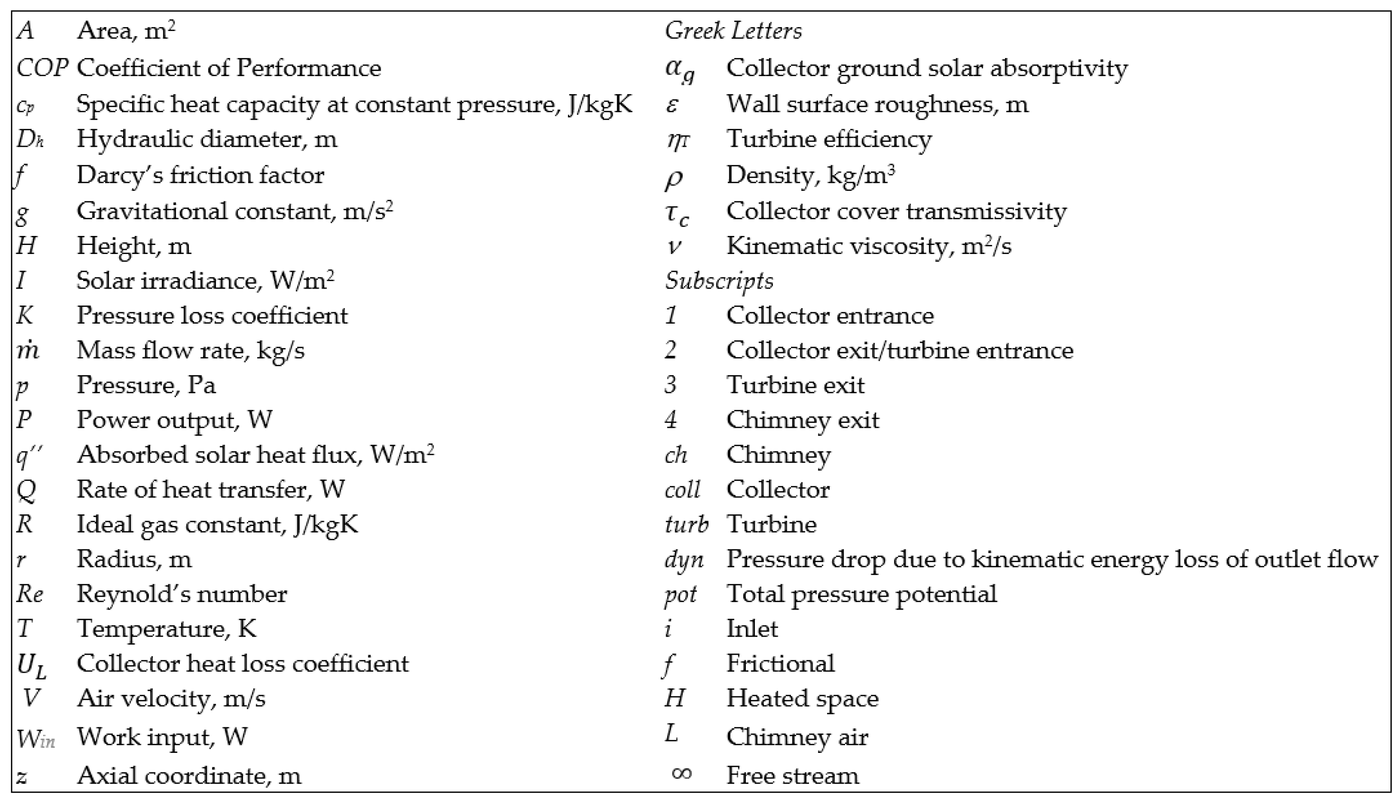
Nomenclature
References
- Yohe, G.; Toth, F.L. Adaptation and the Guardrail Approach to Tolerable Climate Change. Clim. Chang. 2000, 45, 103–128. [CrossRef]
- UNFCCC, “The Paris Agreement,” in Paris Climate Change Conference, Paris, 2015.
- Energy Institute, “Statistical Review of World Energy,” Energy Institute, London, 2023.
- U. N. E. Programme, “Emissions Gap Report,” United Nations Environment Programme, Nairobi, 2023.
- L. D. Vinci, Artist, Design for an airscrew operated smoke-jack. [Art]. Science & Society Picture Library, 1480-1482.
- M. A. d. S. Bernardes, “Solar Chimney Power Plants – Developments and Advancements,” in Solar Energy, Rijeka, InTech, 2010, p. Chapter 9.
- W. Haaf, “Solar Chimneys - Part II: Preliminary Test Results from the Manzanares Pilot Plant,” Harwood Academic Publishers, Reading, 1984.
- J. Schlaich and W. Schiel, “The Solar Chimney: Electricity from the sun,” Schlaich Bergermann und Partner, Stuttgart, Germany, 1995.
- Haaf, W.; Friedrich, K.; Mayr, G.; Schlaich, J. Solar Chimneys Part I: Principle and Construction of the Pilot Plant in Manzanares. Int. J. Sustain. Energy 1983, 2, 3–20. [CrossRef]
- T. K. Grose, “Solar Chimneys Can Convert Hot Air to Energy, But Is Funding a Mirage?,” National Geographic, 17 April 2014.
- N. P. Stoianoff, L. Kreiser, B. Butcher, J. E. Milne and H. Ashiabor, Green Fiscal Reform for a Sustainable Future: Reform, Innovation and Renewable Energy, Cheltenham: Edward Elgar Publishing, 2016.
- Ghalamchi, M.; Kasaeian, A.; Mirzahosseini, A.H. An experimental study on the thermal performance of a solar chimney with different dimensional parameters. Renew. Energy 2016, 91, 477–483. [CrossRef]
- Lal, S.; Kaushik, S.; Hans, R. Experimental investigation and CFD simulation studies of a laboratory scale solar chimney for power generation. Sustain. Energy Technol. Assessments 2016, 13, 13–22. [CrossRef]
- the Faculty of Energy Engineering; Mekhail, T.; Rekaby, A.; Fathy, M.; Bassily, M.; Harte, R. Experimental and Theoretical Performance of Mini Solar Chimney Power Plant. J. Clean Energy Technol. 2017, 5, 294–298. [CrossRef]
- Koonsrisuk, S. Lorente and A. Bejan, “Constructal solar chimney configuration,” International Journal of Heat and Mass Transfer, vol. 53, pp. 327-333, 2010.
- Raney, S.M.; Brooks, J.R.; Schaffer, J.P.; French, J.J. Experimental Validation of Solar Chimney Performance Models and Operational Characteristics for Small Scale Remote Applications. ASME 2012 6th International Conference on Energy Sustainability collocated with the ASME 2012 10th International Conference on Fuel Cell Science, Engineering and Technology, United States; pp. 27–32.
- Zhou, X.; Yang, J.; Xiao, B.; Hou, G.; Xing, F. Analysis of chimney height for solar chimney power plant. Appl. Therm. Eng. 2008, 29, 178–185. [CrossRef]
- Cuce, E.; Cuce, P.M.; Sen, H. A thorough performance assessment of solar chimney power plants: Case study for Manzanares. Clean. Eng. Technol. 2020, 1, 100026. [CrossRef]
- Koonsrisuk, A.; Chitsomboon, T. Mathematical modeling of solar chimney power plants. Energy 2013, 51, 314–322. [CrossRef]
- Setareh, M. Comprehensive mathematical study on solar chimney powerplant. Renew. Energy 2021, 175, 470–485. [CrossRef]
- H. Kreetz, “Theoretische Untersuchungen und Auslegung eines temporären Wasserspeichers für das Aufwindkraftwerk,” Energien-EVUR, Technical University Berlin, Berling, 1997.
- D. Pritam and V. Chandramohan, “A review on solar updraft tower plant technology: Thermodynamic analysis, worldwide status, recent advances, major challenges and opportunities,” Sustainable Energy Technologies and Assessments, vol. 52, 2022.
- Strobel, C.S.; Moura, L.M.; Catapan, M.F. Technical feasibility analysis of the use of solar chimneys in Brazil. Rev. Bras. de Planej. e Desenvolv. 2020, 9, 450–467. [CrossRef]
- Dhimish, M.; Mather, P. Exploratory evaluation of solar radiation and ambient temperature in twenty locations distributed in United Kingdom. Urban Clim. 2018, 27, 179–192. [CrossRef]
- British Gas, “What is the average energy bill in Great Britain?,” April 2024. [Online]. Available: https://www.britishgas.co.uk/energy/guides/average-bill. [Accessed 20 November 2024].
- D. Crismale, “How much energy does the average home use?,” Finder, 19 January 2024. [Online]. Available: https://www.finder.com.au/energy/how-much-energy-does-the-average-home-use. [Accessed 20 November 2024].
- Tiedemann, K. Performance standards and residential energy efficiency in Egypt. WASTE MANAGEMENT 2006.
- Statista, “Residential electricity consumption in Brazil from 2013 to 2022,” 12 July 2023. [Online]. Available: https://www.statista.com/statistics/985975/brazil-residential-electricity-consumption/#:~:text=In%202022%2C%20the%20residential%20electricity,percent%20of%20Brazil's%20electricity%20consumption. [Accessed 20 November 2024].
- M. Zambrano-Monserrate and M. Ruano, “Sociodemographic drivers and interconnected energy-saving practices: insights from Ecuador's household sector,” Management of Environmental Quality, vol. 35, no. 4, pp. 885-902, 2024.
- Solcast, “Historical Time Series,” DNV Company, 2024. [Online]. Available: https://solcast.com. [Accessed 20 November 2024].
- Cuce, P.M.; Cuce, E.; Sen, H. Improving Electricity Production in Solar Chimney Power Plants with Sloping Ground Design: An Extensive CFD Research. J. Sol. Energy Res. Updat. 2020, 7, 122–131. [CrossRef]
- Fluri, T.; von Backström, T. Comparison of modelling approaches and layouts for solar chimney turbines. Sol. Energy 2008, 82, 239–246. [CrossRef]
- Pretorius, J.P.; Kröger, D.G. Solar Chimney Power Plant Performance. J. Sol. Energy Eng. 2006, 128, 302–311. [CrossRef]
- Haaland, S.E. Simple and Explicit Formulas for the Friction Factor in Turbulent Pipe Flow. J. Fluids Eng. 1983, 105, 89–90. [CrossRef]
- Dawood, A.O.; Sangoor, A.J.; Al-Rkaby, A.H. Behavior of tall masonry chimneys under wind loadings using CFD technique. Case Stud. Constr. Mater. 2020, 13, e00451. [CrossRef]
- H. Sharon, “ A detailed review on sole and hybrid solar chimney based sustainable ventilation, power generation, and potable water production systems,” Energy Nexus, vol. 10, 2023.
- P. Singh, A. Kumar, Akshayveer and O. Singh, “Performance enhancement strategies of a hybrid solar chimney power plant T integrated with photovoltaic panel,” Energy Conversion and Management, vol. 218, 2020.
- Australian Bureau of Statistics, “New houses being built on smaller blocks.,” 7 June 2022. [Online]. Available: https://www.abs.gov.au/articles/new-houses-being-built-smaller-blocks#cite-window1. [Accessed 20 November 2024.
- The Engineering Toolbox, “ir - Density, Specific Weight and Thermal Expansion Coefficient vs. Temperature and Pressure,” 2003. [Online]. Available: https://www.engineeringtoolbox.com/air-density-specific-weight-d_600.html. [Accessed 20 November 2024].
- Green Match, “Best Air Source Heat Pump Manufacturers UK 2024,” 3 April 2024. [Online]. Available: https://www.greenmatch.co.uk/heat-pumps/manufacturers. [Accessed 20 November 2024].
- glassglobal, “Glass Directory,” 2024. [Online]. Available: https://www.glassglobal.com/directory/glass/. [Accessed 20 November 2024].
- The Trade Vision, “Ecuador Suppliers of plastic sheets,” 2024. [Online]. Available: https://www.thetradevision.com/global/plastic-sheets-suppliers-in-ecuador. [Accessed 20 November 2024].
- Volza Grow Global, “Pvc sheet export data of Australia,” 2024. [Online]. Available: https://www.volza.com/p/pvc-sheet/export/export-from-australia/. [Accessed 20 November 2024].
- OEC, “Bitumen and asphalt,” 2022. [Online]. Available: https://oec.world/en/profile/hs/bitumen-and-asphalt. [Accessed 20 November 2024].
- Viva Energy, “Geelong Refinery,” 2024. [Online]. Available: https://www.vivaenergy.com.au/operations/geelong. [Accessed 20 November 2024].
- International Trade Administration, “Ecuador - Country Commercial Guide,” 8 February 2024. [Online]. Available: https://www.trade.gov/country-commercial-guides/ecuador-mining#:~:text=Ecuador%20enjoys%20excellent%20mineral%20resources,increasing%2033%20percent%20in%20mining. [Accessed 20 November 2024].
- Australian Government: Geoscience Australia, “Australian mineral facts,” 19 April 2024. [Online]. Available: https://www.ga.gov.au/education/minerals-energy/australian-mineral-facts. [Accessed 20 November 2024].
- Echo Precast Engineering, “Uncharted territory for precast technology – first precast concrete plant opened in Ecuador,” Concrete Plant International, vol. 5, pp. 184-186, 2016.
- National Precast, “Find-a-master precaster,” 2024. [Online]. Available: https://nationalprecast.com.au/tools/find-a-master-precaster/. [Accessed 20 November 2024].
- ANSYS Granta EduPack, GRANTA EduPack software, Cambridge: ANSYS, 2022.
- Krishnan, A.R.; D, K. Influence of heat absorber materials sand, soil and paraffin wax in solar still on sustainable water distillation. Case Stud. Chem. Environ. Eng. 2023, 8. [CrossRef]
- The Engineering Toolbox, “Absorbed Solar Radiation,” 2009. [Online]. Available: https://www.engineeringtoolbox.com/solar-radiation-absorbed-materials-d_1568.html. [Accessed 20 November 2024].
- Adedeji, J. Aweda and O. Lasode, “Estimation of Service Life for a Solar Chimney-Collector System,” Lecture Notes in Engineering and Computer Science., 2010.
- EPA. United States Environmental Protection Agency. Greenhouse Gas Equivalencies Calculator. Available online https://www.epa.gov/energy/greenhouse-gas-equivalencies-calculator (accessed on 2 February 2018).
- Z. Xinping, Y. Jiakuan, X. Bo and H. Guoxiang, “Experimental study of temperature field in a solar chimney power setup,” Applied Thermal Engineering, vol. 27, no. 11-12, pp. 2044-2050, 2007.
Figure 1.
(a) Basic design of a Solar Chimney Power Plant (SCPP); (b) Schematic showing its operation.
Figure 1.
(a) Basic design of a Solar Chimney Power Plant (SCPP); (b) Schematic showing its operation.
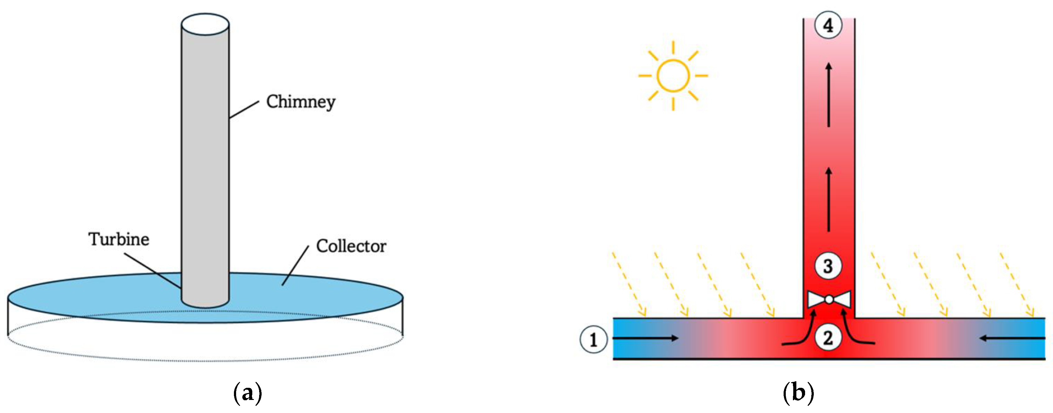
Figure 2.
SCPP prototype in Manzanares, Spain [8].
Figure 2.
SCPP prototype in Manzanares, Spain [8].
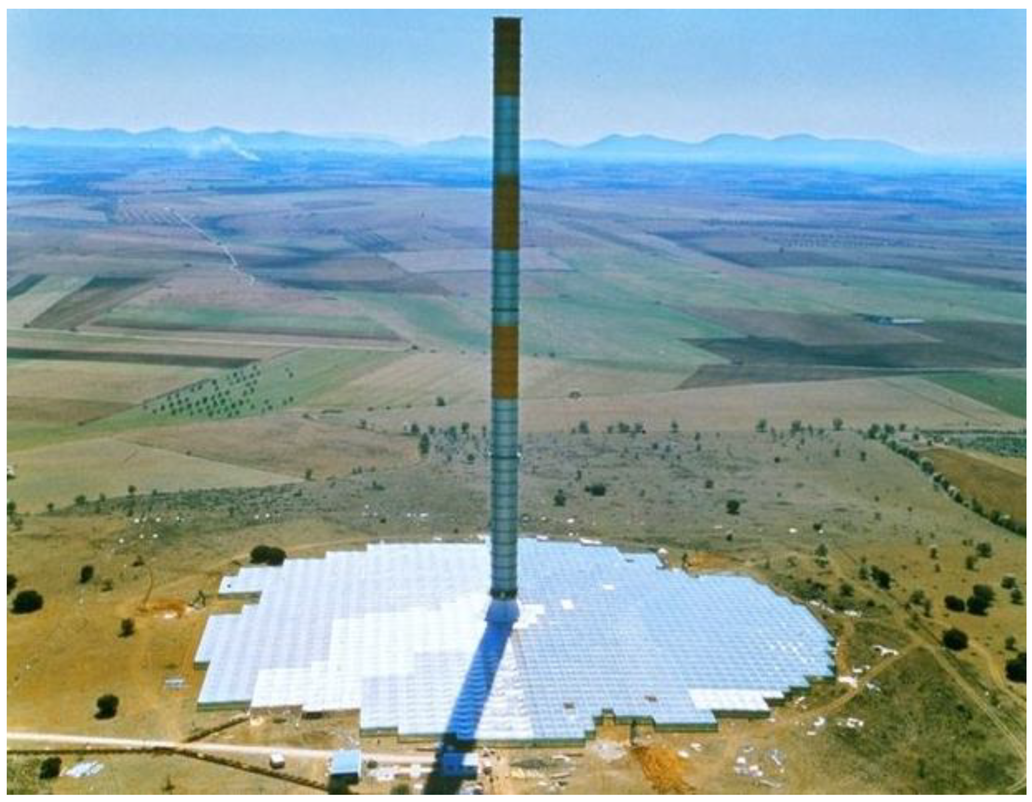
Figure 3.
World map indicating the locations to be studied.

Figure 4.
Average 4-weekly (a) ambient temperature and (b) Global Horizontal Irradiance (GHI) for the five locations in 2023.
Figure 4.
Average 4-weekly (a) ambient temperature and (b) Global Horizontal Irradiance (GHI) for the five locations in 2023.
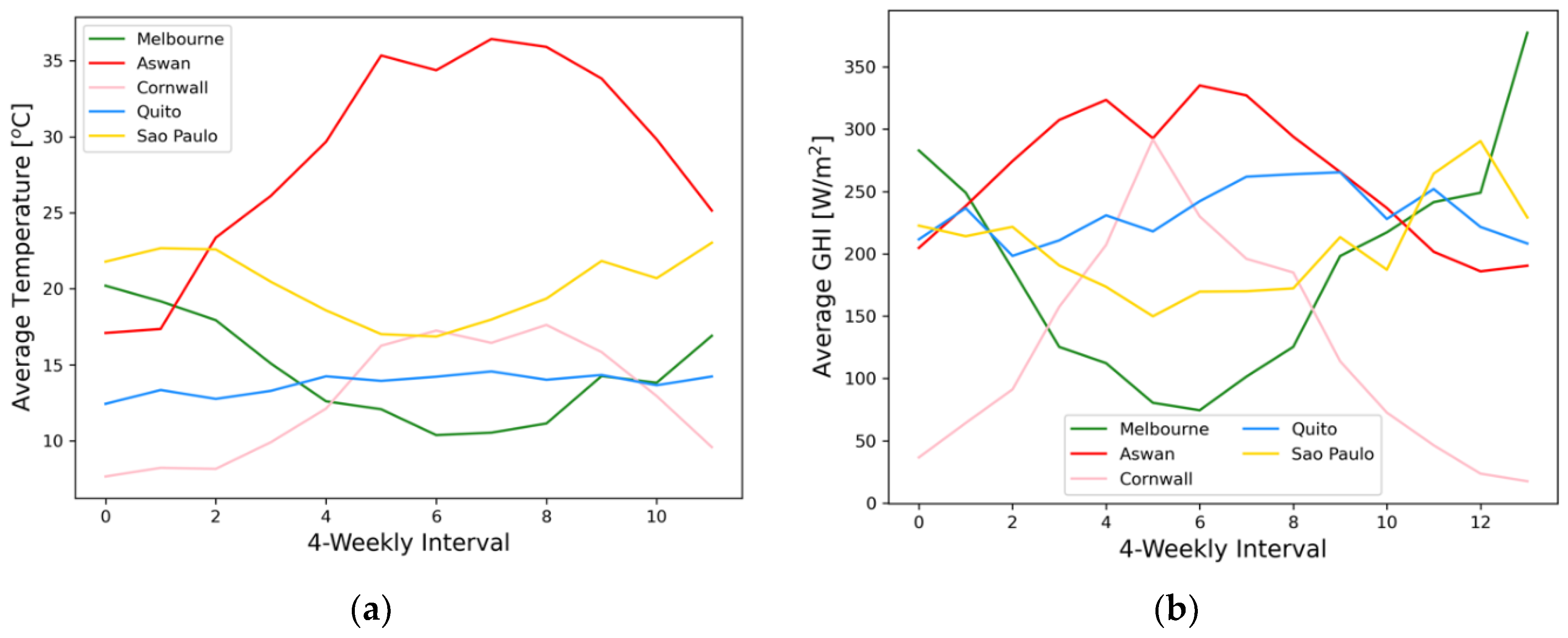
Figure 5.
Flowchart of the computational procedure.
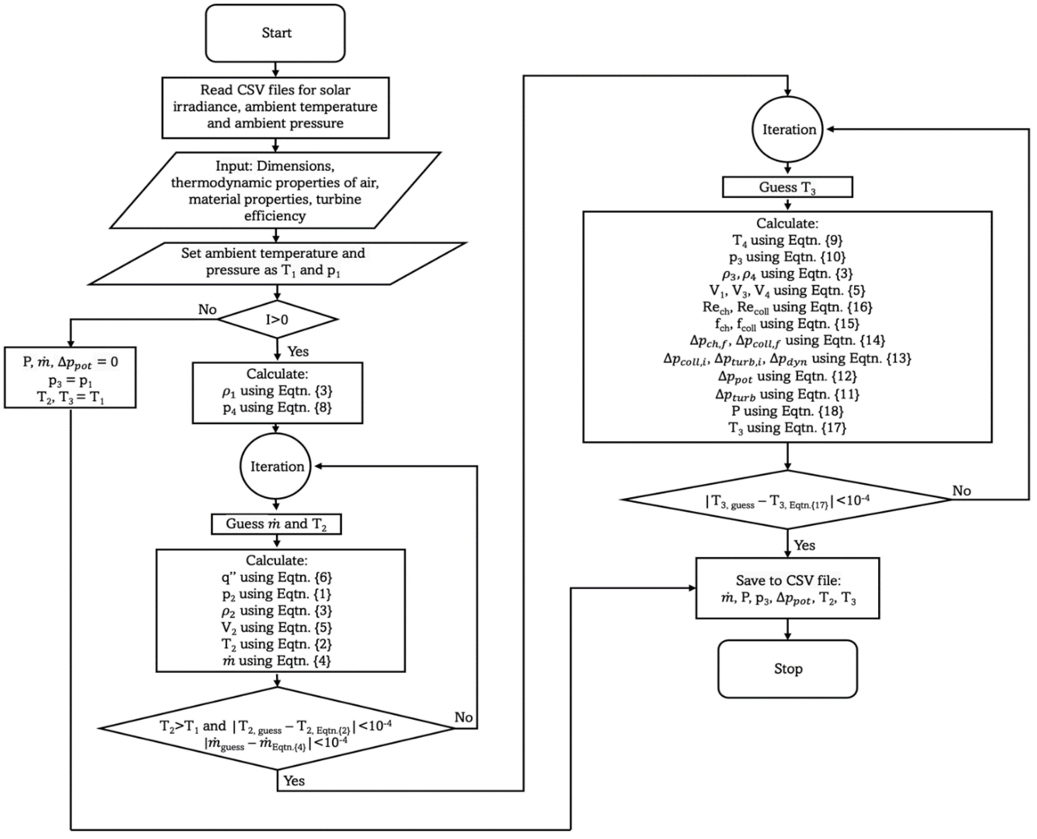
Figure 6.
Graph to show the effect on the power output by varying input parameters.
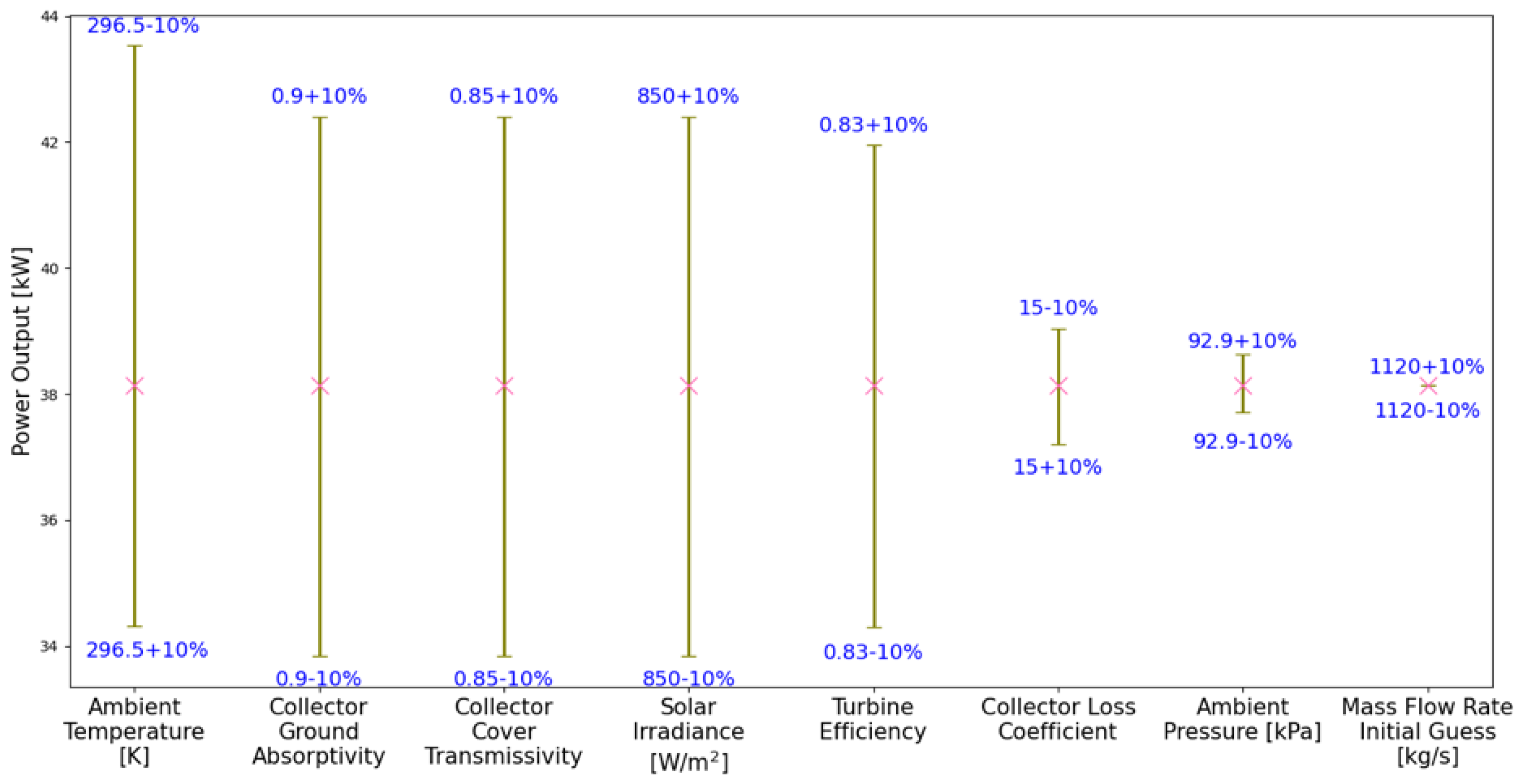
Figure 7.
(a) Peak power output in 2023 at all locations. (b) Plot of GHI and ambient temperature over 24 hours on 29/12/23 in Melbourne.
Figure 7.
(a) Peak power output in 2023 at all locations. (b) Plot of GHI and ambient temperature over 24 hours on 29/12/23 in Melbourne.
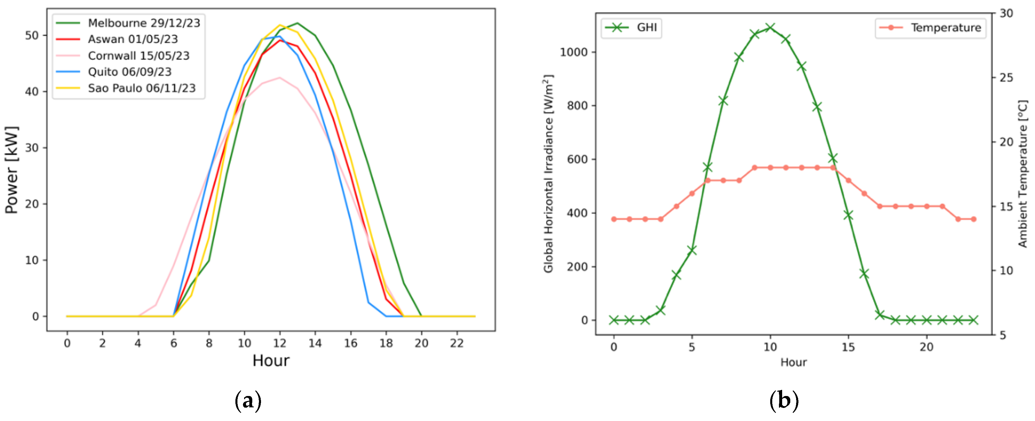
Figure 8.
Average 4-weekly power output in (a) 2007 and (b) 2023.
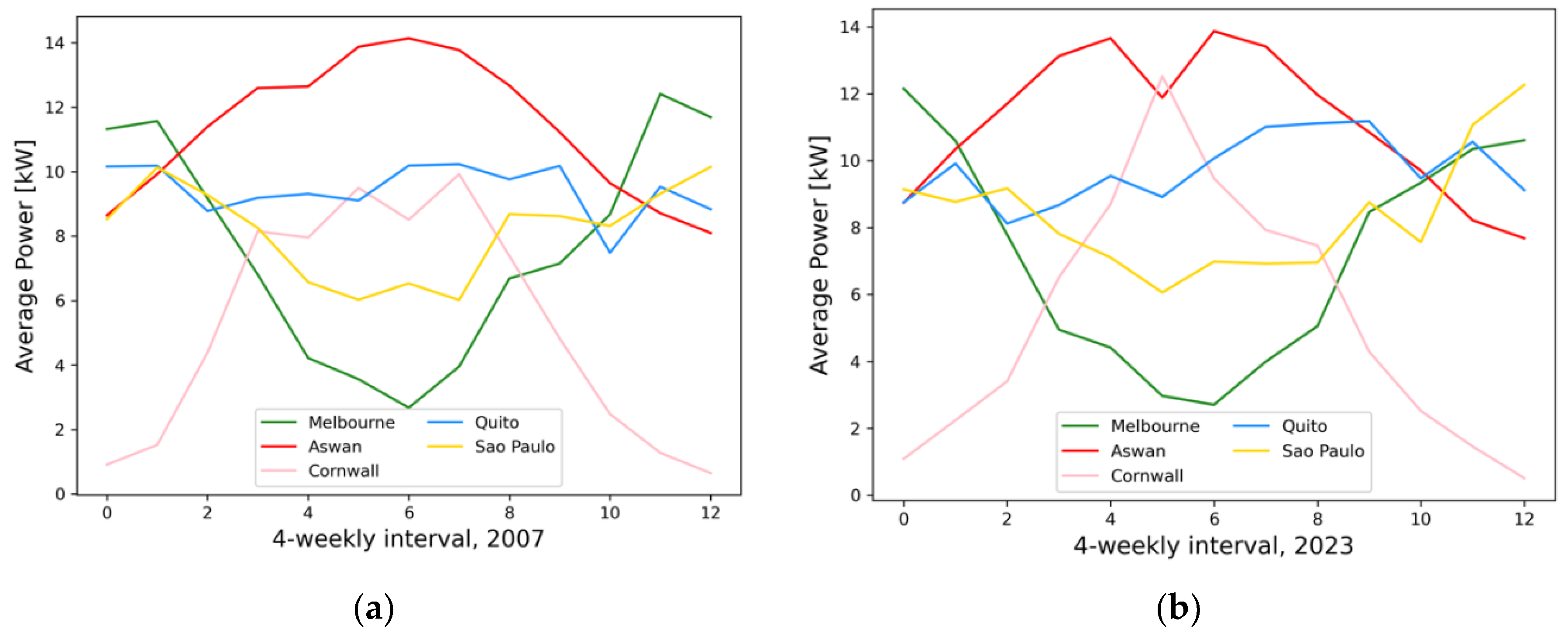
Figure 9.
Plots to show annual energy produced when varying the dimensions of individual parameters, using 2023 Aswan meteorological data and Manzanares SCPP dimensions.
Figure 9.
Plots to show annual energy produced when varying the dimensions of individual parameters, using 2023 Aswan meteorological data and Manzanares SCPP dimensions.
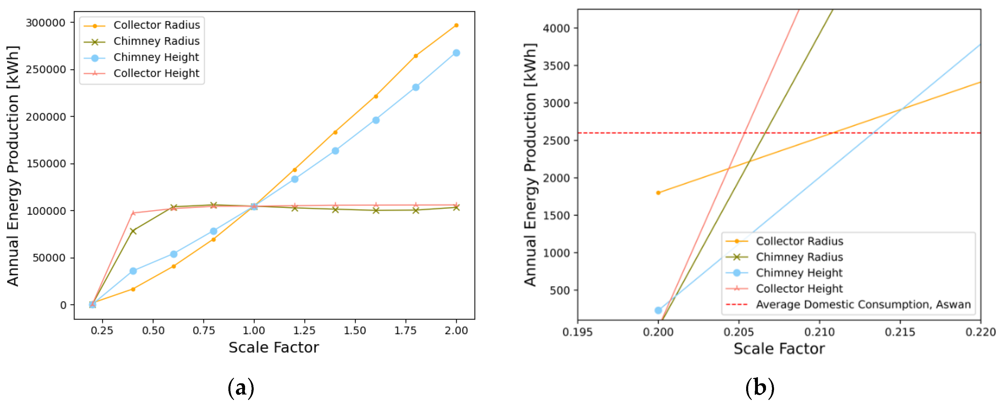
Figure 10.
Plots showing annual energy produced when varying the ratio of (a) the chimney height to the collector radius of 122m and (b) the collector radius to the chimney height of 194.6m, using 2023 meteorological data and all other dimensions consistent with the Manzanares SCPP.
Figure 10.
Plots showing annual energy produced when varying the ratio of (a) the chimney height to the collector radius of 122m and (b) the collector radius to the chimney height of 194.6m, using 2023 meteorological data and all other dimensions consistent with the Manzanares SCPP.
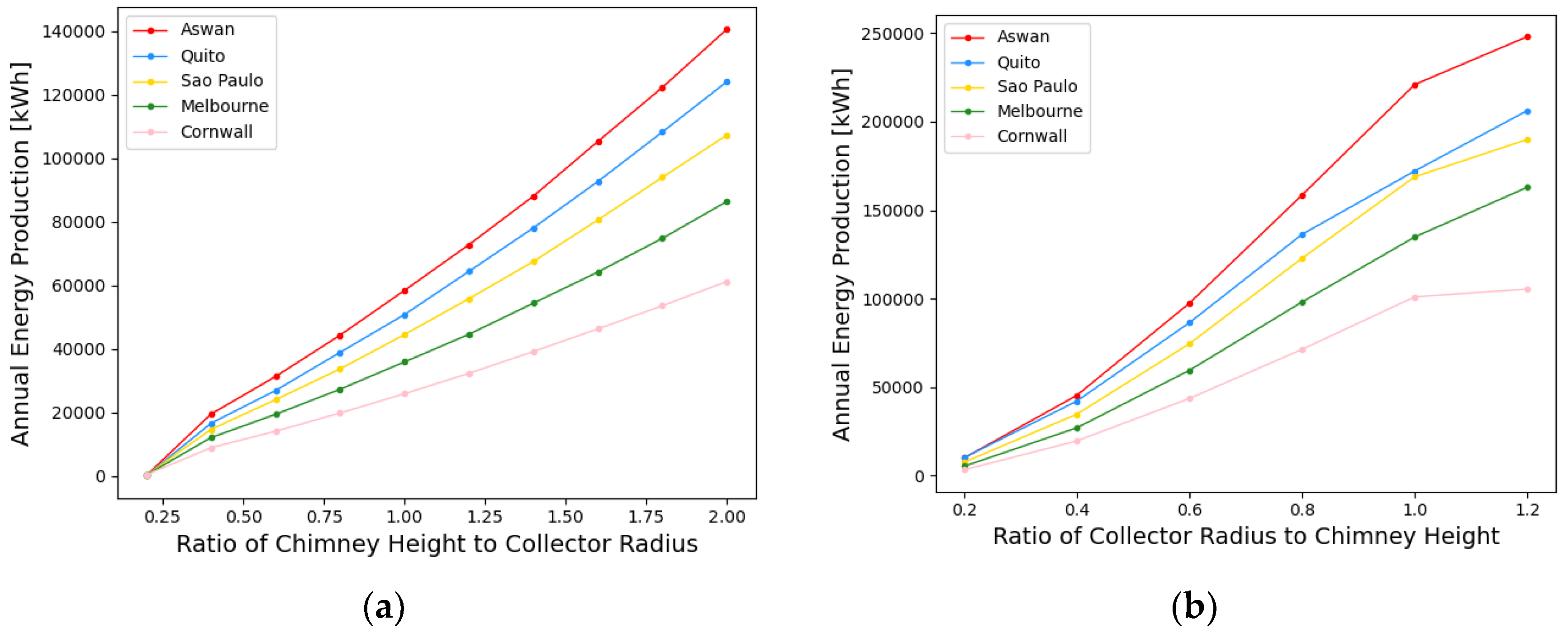
Figure 11.
Plot to show the effect on the 2023 annual energy production with a varying dimensional scale factor.
Figure 11.
Plot to show the effect on the 2023 annual energy production with a varying dimensional scale factor.
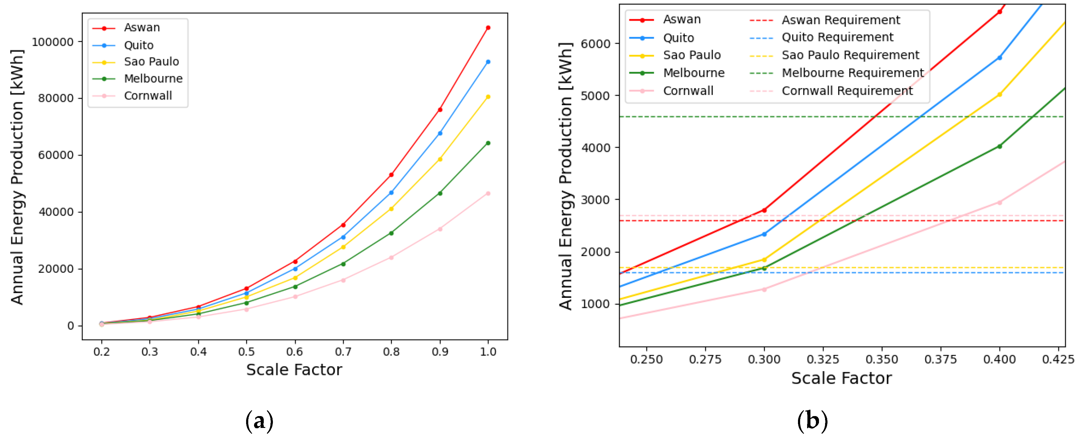
Figure 12.
Plot to show the relationship and regression models in (a) 2007 and (b) 2023, between required chimney height and collector radius to achieve the average annual energy production at each location.
Figure 12.
Plot to show the relationship and regression models in (a) 2007 and (b) 2023, between required chimney height and collector radius to achieve the average annual energy production at each location.
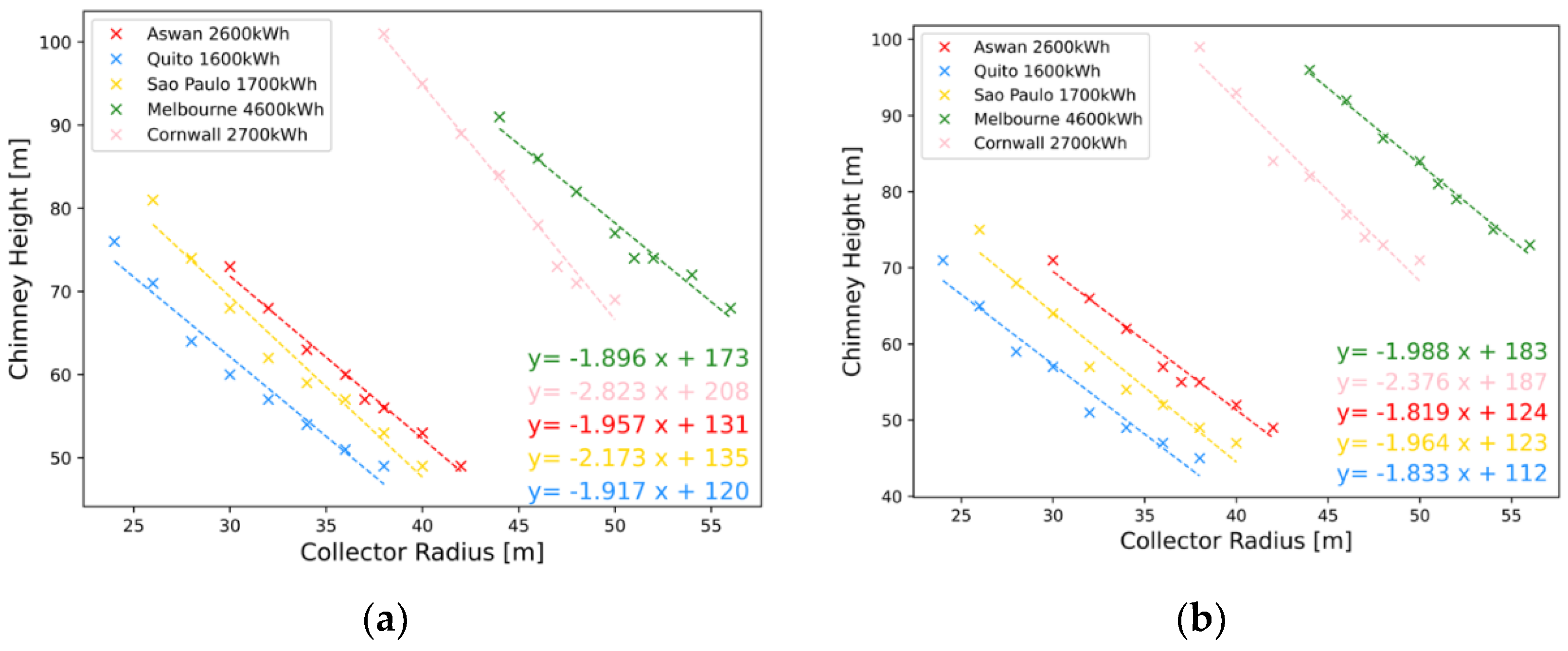
Figure 13.
Comparison of required chimney dimensions by location for a 70m chimney height in 2023.
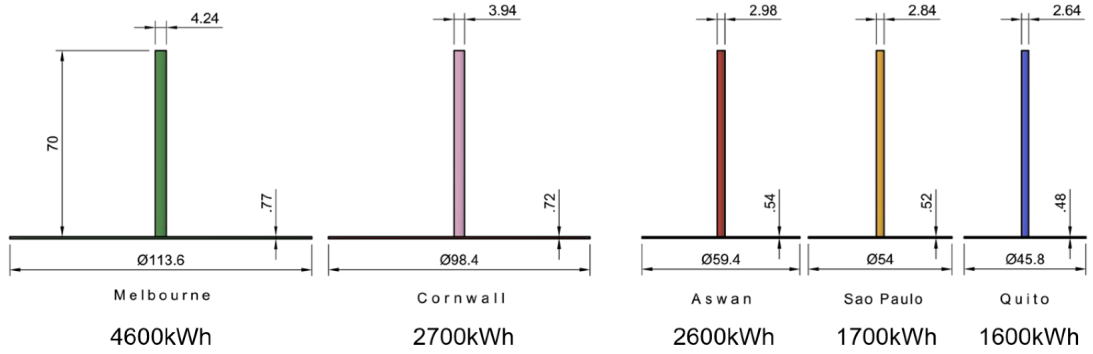
Figure 14.
Plot to show the (a) average energy production and (b) maximum power output for each plant with a 70m chimney height in 2023.
Figure 14.
Plot to show the (a) average energy production and (b) maximum power output for each plant with a 70m chimney height in 2023.
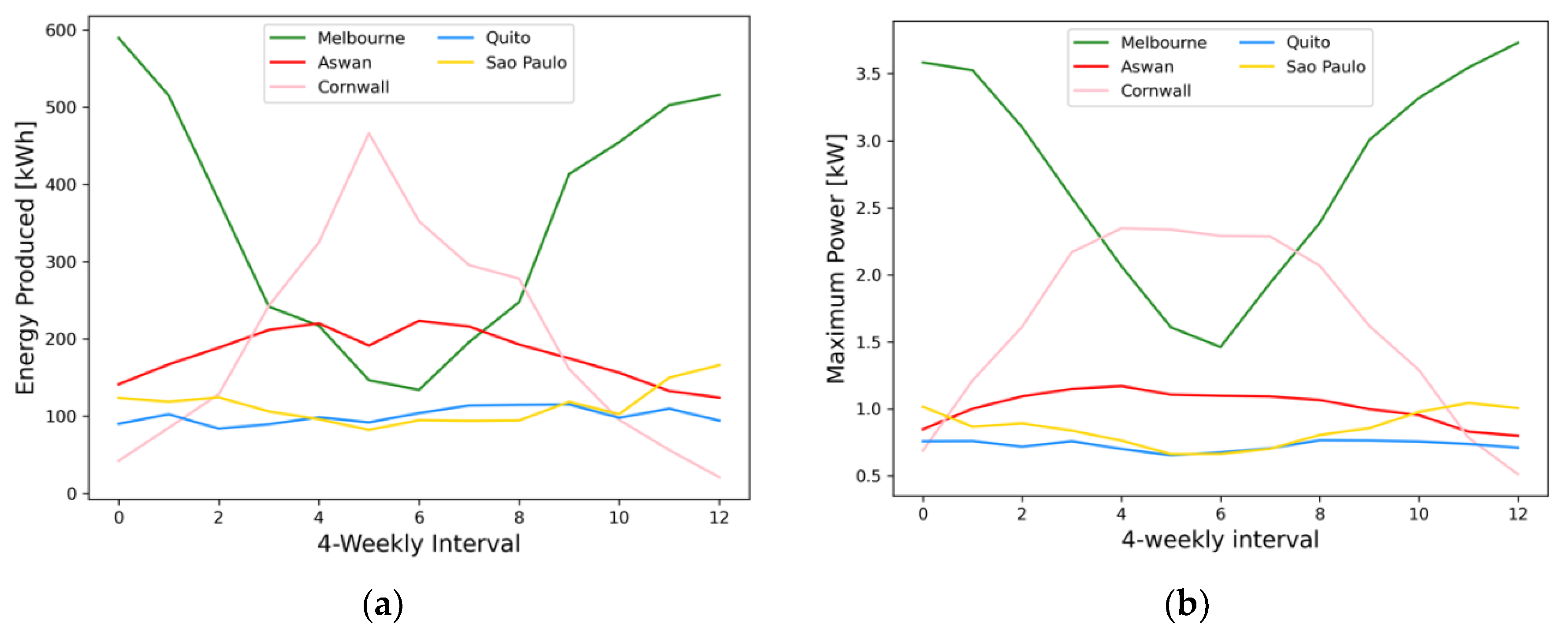
Figure 15.
Comparison of CO2 footprint of a SCPP in Quito and Melbourne, based on locally available materials.
Figure 15.
Comparison of CO2 footprint of a SCPP in Quito and Melbourne, based on locally available materials.
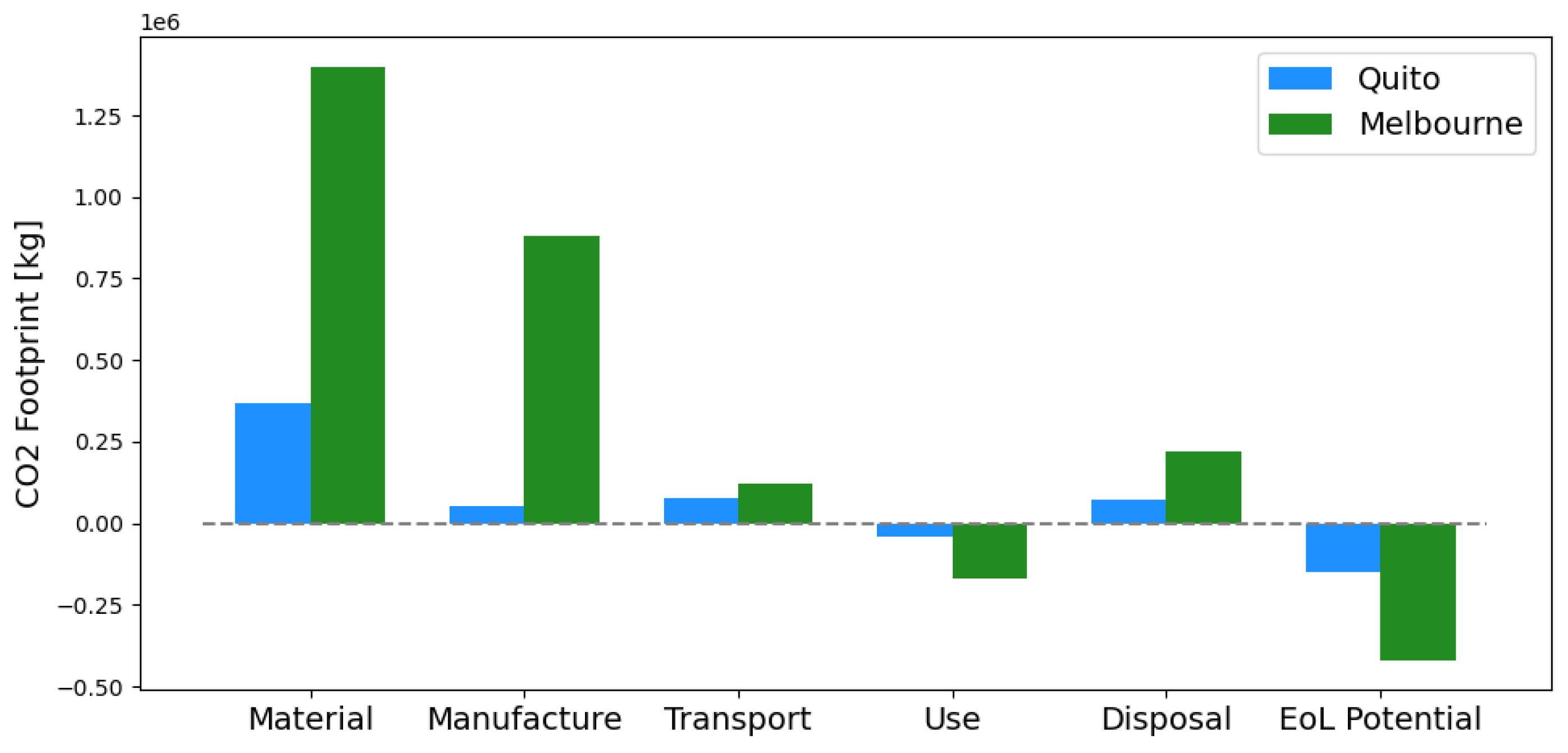

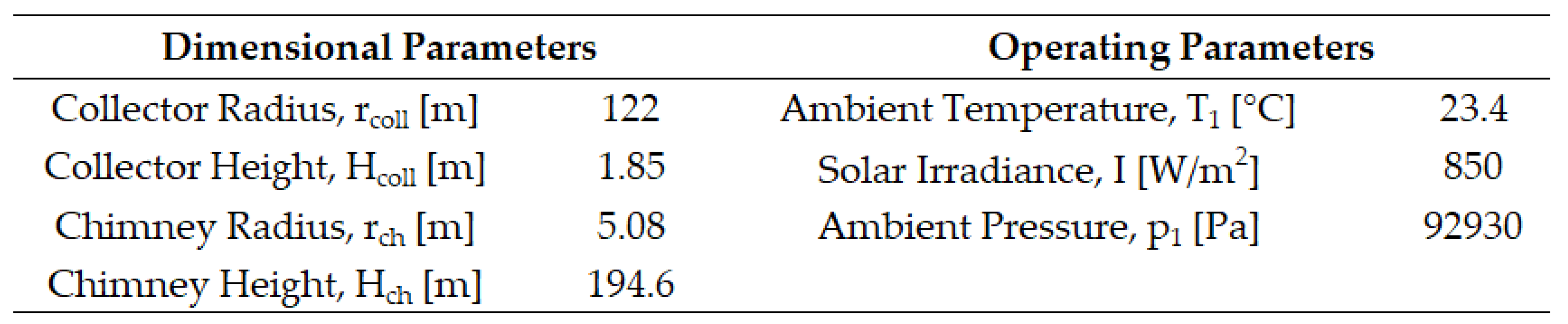
Table 2.
Reported methods for calculating power output.
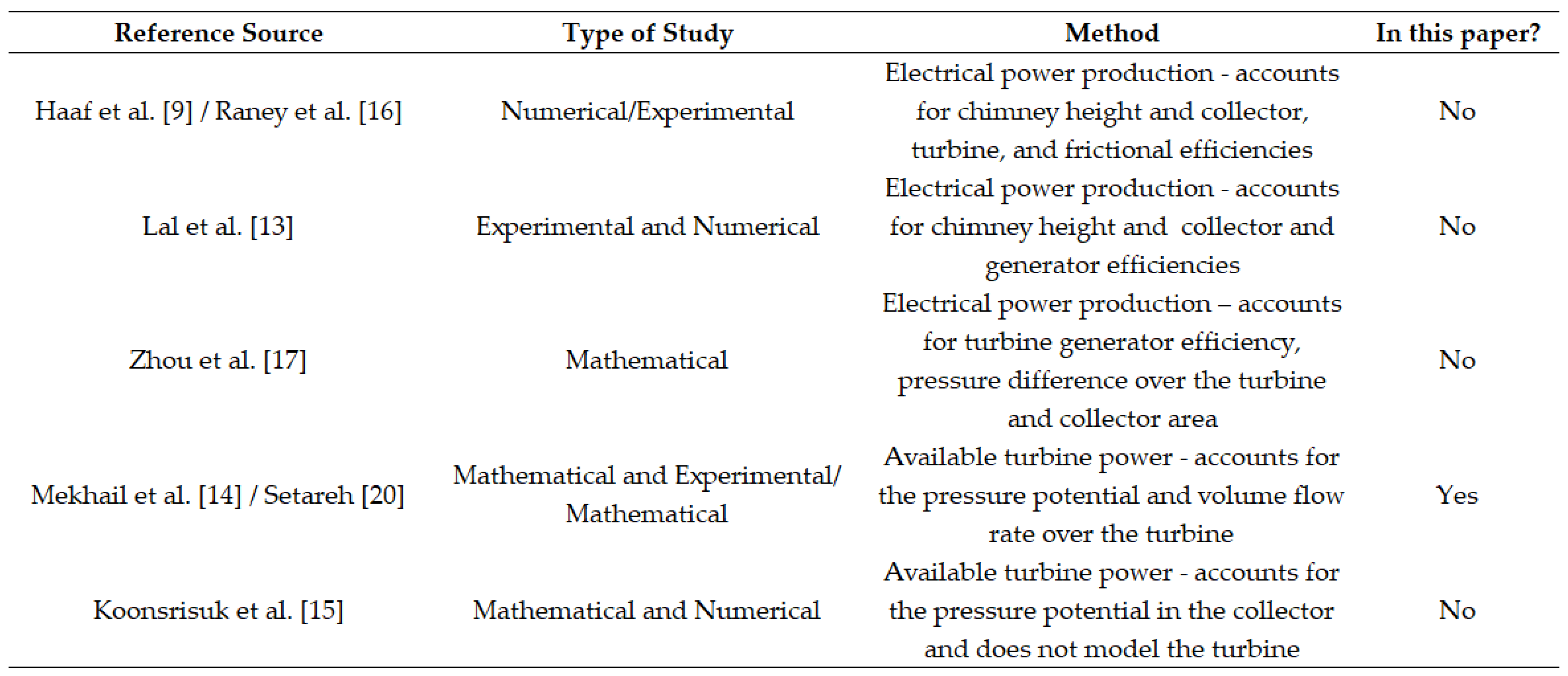
Table 3.
Average annual domestic electricity consumption.

Table 4.
Properties of air used in the analysis [19].
Table 4.
Properties of air used in the analysis [19].
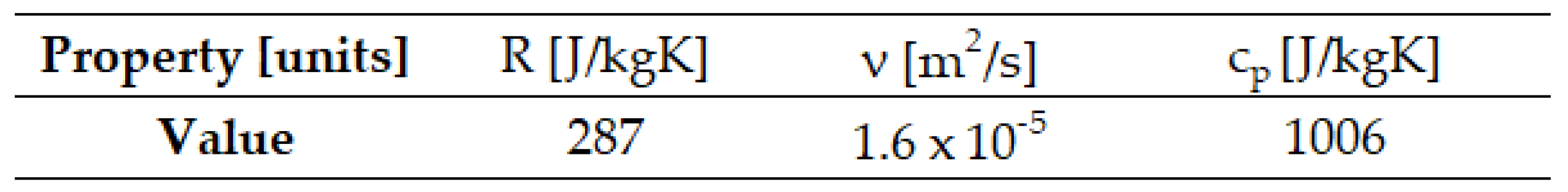
Table 5.
Comparison of measured experimental outputs and calculated theoretical outputs.
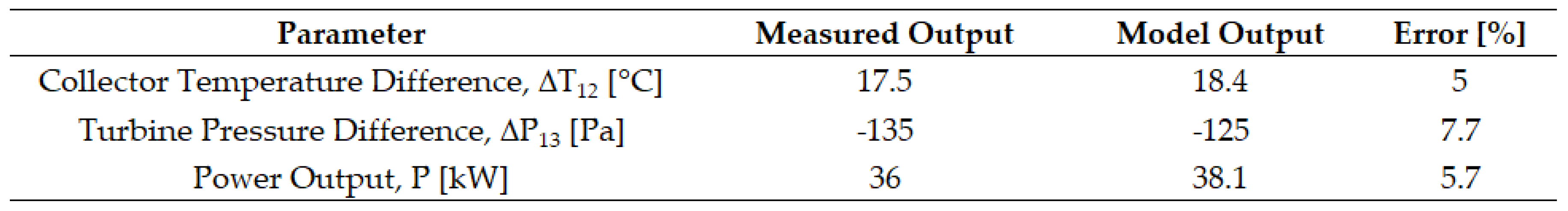
Table 6.
Peak power output data 2023.
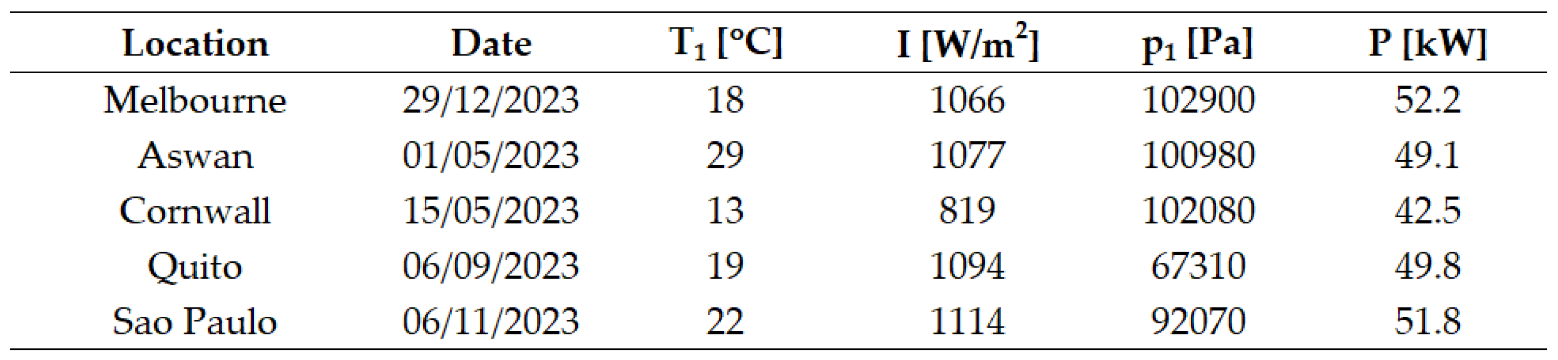
Table 7.
Annual energy production in kWh in 2007 and 2023.
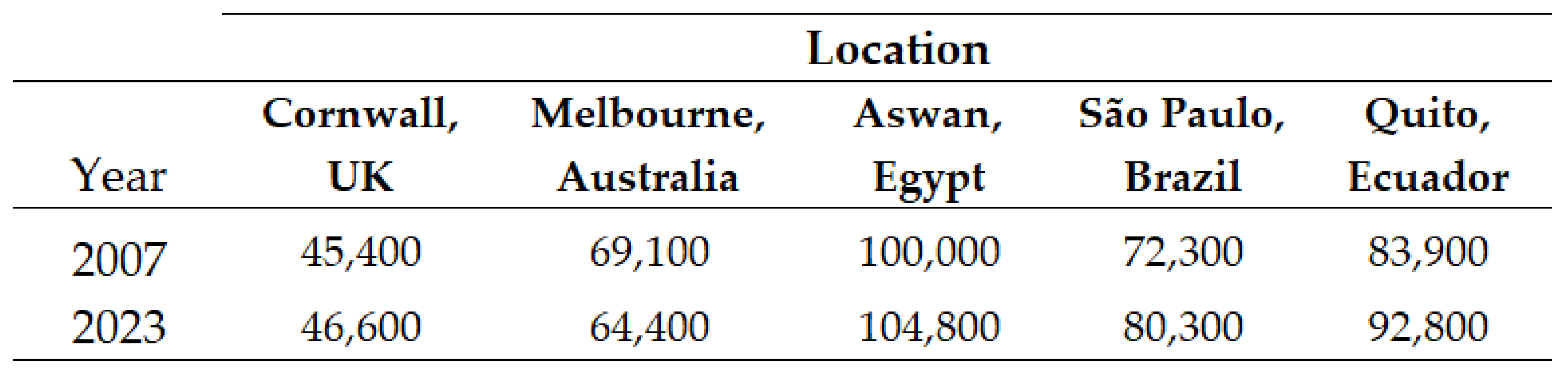
Table 8.
Minimum scale factor of the Manzanares SCPP to achieve the average annual household energy consumption by location.
Table 8.
Minimum scale factor of the Manzanares SCPP to achieve the average annual household energy consumption by location.
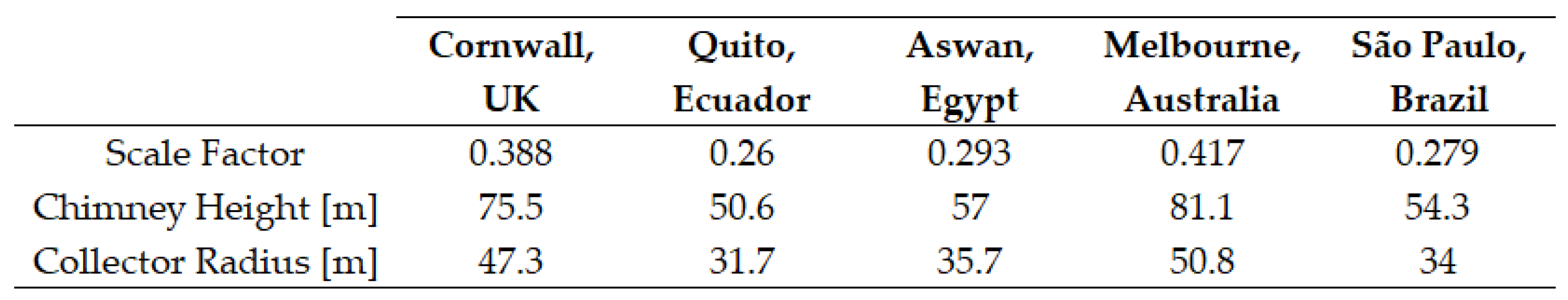
Table 9.
Correlation coefficient of the linear relationship between chimney height and collector radius in 2007 and 2023.
Table 9.
Correlation coefficient of the linear relationship between chimney height and collector radius in 2007 and 2023.
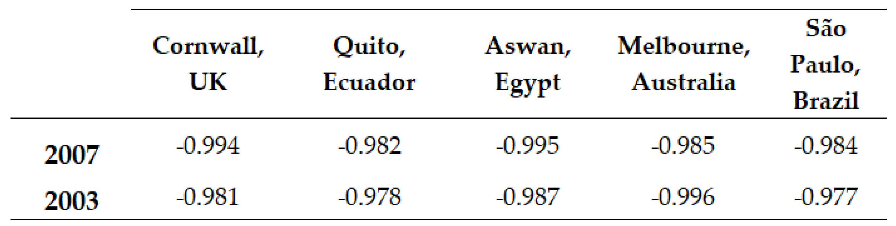
Table 10.
Percentage change in the size of the collector radius from 2007 to 2023 for a 70m chimney height.
Table 10.
Percentage change in the size of the collector radius from 2007 to 2023 for a 70m chimney height.
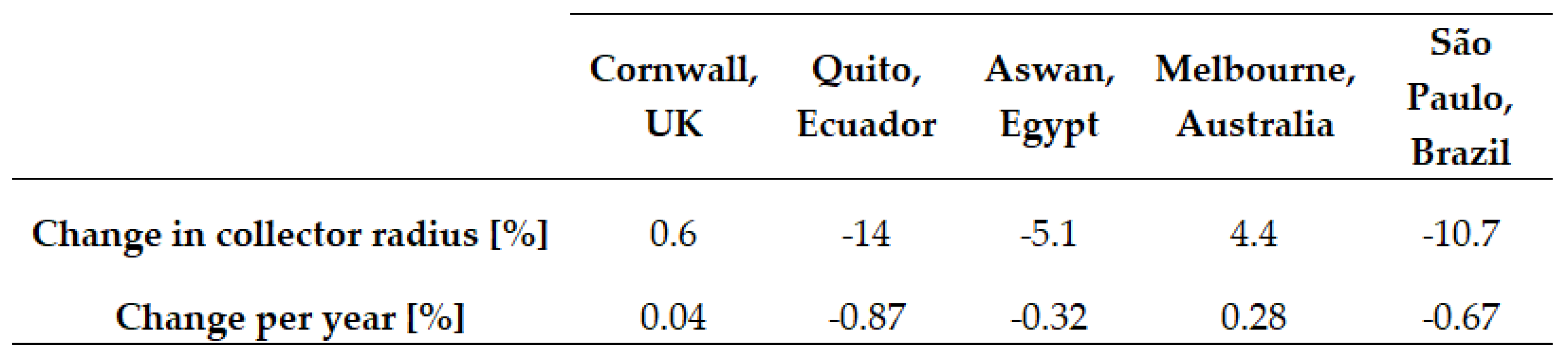
Table 11.
Multi Criteria Decision Analysis for hybridisation study of the SCPP system.
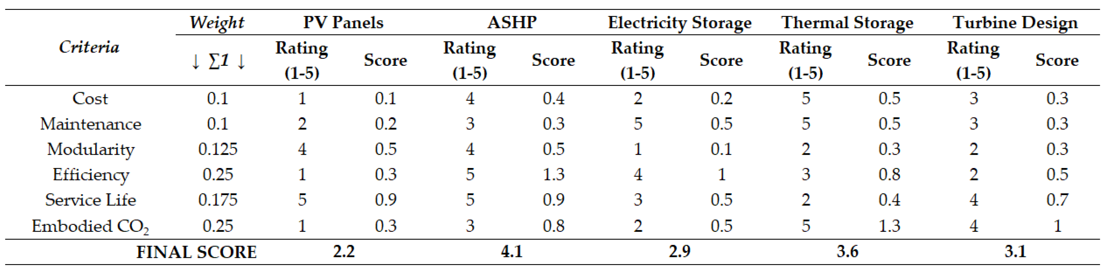
Table 12.
Parameters from Melbourne for ASHP calculations.

Table 13.
Melbourne ASHP calculation results.
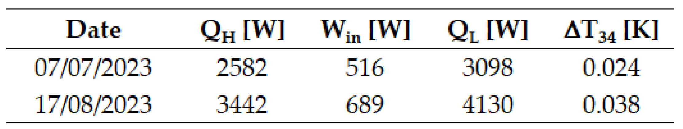
Table 14.
Availability of materials in Quito and Melbourne.
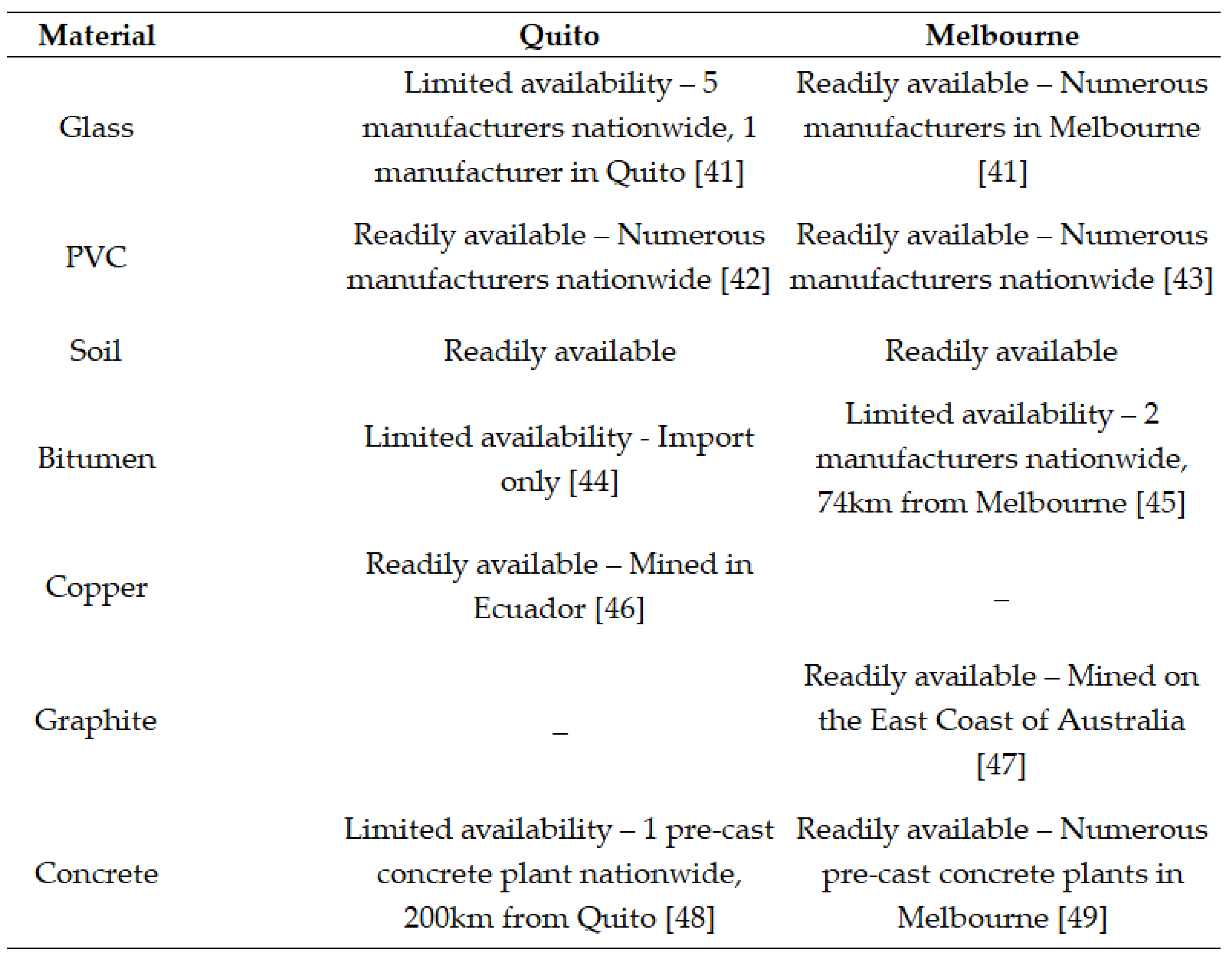
Table 15.
Properties of collector materials.
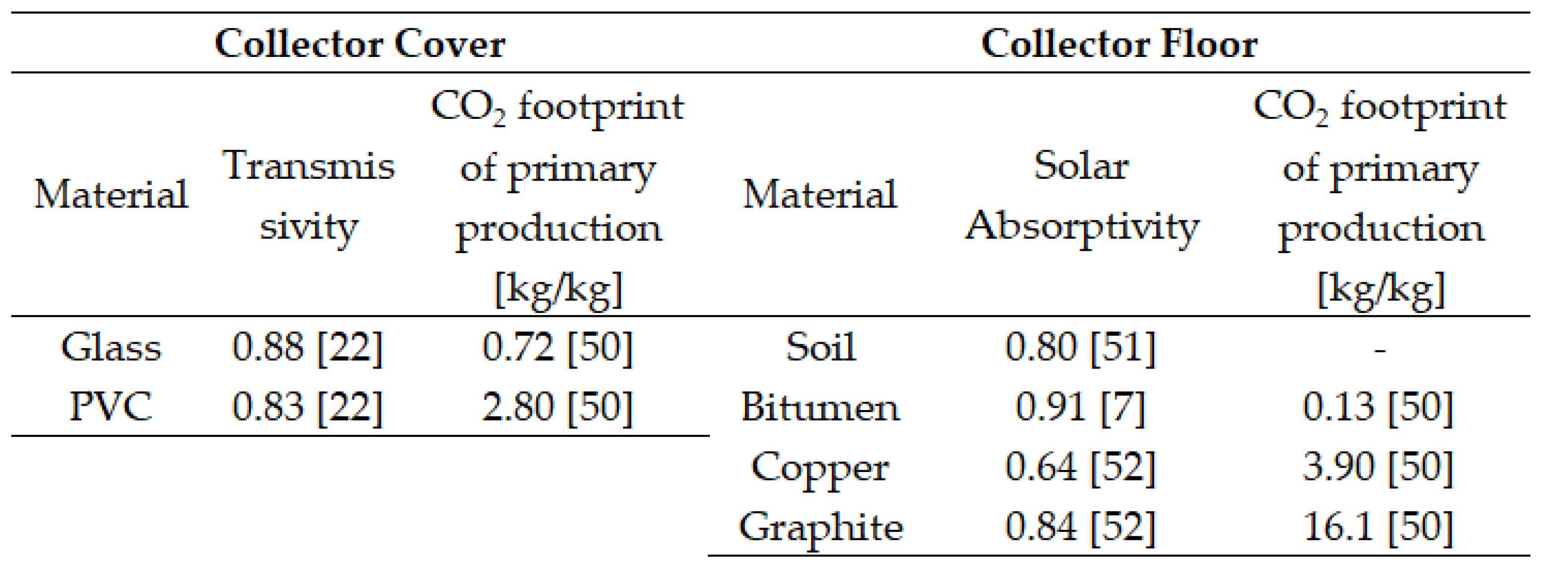
Table 16.
Annual energy output in 2023 with different materials.
Disclaimer/Publisher’s Note: The statements, opinions and data contained in all publications are solely those of the individual author(s) and contributor(s) and not of MDPI and/or the editor(s). MDPI and/or the editor(s) disclaim responsibility for any injury to people or property resulting from any ideas, methods, instructions or products referred to in the content. |
© 2024 by the authors. Licensee MDPI, Basel, Switzerland. This article is an open access article distributed under the terms and conditions of the Creative Commons Attribution (CC BY) license (http://creativecommons.org/licenses/by/4.0/).
Copyright: This open access article is published under a Creative Commons CC BY 4.0 license, which permit the free download, distribution, and reuse, provided that the author and preprint are cited in any reuse.


