
Submitted:
25 November 2024
Posted:
26 November 2024
You are already at the latest version
Abstract
This study investigates the impact of various irrigation regimes and organic fertilizers on olive cultivation productivity and environmental sustainability. Experimental results showed that olive trees fertilized with biochar yielded an average of 2640 kg ha-1, while those fertilized with a commercial product based on dry blood resulted in lower yields of 1820 kg ha-1. Significant productivity gains were observed under irrigation, particularly with the fully watered regime, which nearly doubled yields compared to non-irrigated trees. The study also highlighted the influence of irrigation on water use efficiency, with water consumption metrics varying notably among different fertilization treatments. The water footprint analysis indicated that the most sustainable option, characterized by the lowest water footprint, did not consistently align with productivity gains, emphasizing the need for integrated management strategies. An analysis of marginal irrigation use efficiency revealed that optimizing irrigation volumes improved productivity while providing substantial water savings. A scoring system was employed to standardize various parameters, enabling direct comparisons of irrigation and fertilization treatments. Ultimately, the results suggested that biochar, in combination with deficit irrigation strategies, could enhance both productivity and sustainability in olive farming, with the strategy of ceasing irrigation at the pit hardening phase achieving the highest aggregated score for management effectiveness. These findings underscore the importance of optimizing irrigation and fertilization practices to promote environmentally sustainable agricultural systems in Mediterranean climates.
Keywords:
Keywords water use
; CropWat
; aggregated metric
; sustainability
1. Introduction
The agricultural sector is crucial for ensuring global food security, yet it imposes substantial environmental burdens, particularly on freshwater resources. Agricultural activities account for approximately 70% of global freshwater withdrawals, with this figure rising to over 80% in water-scarce areas, such as warm temperate climate areas [1]. This is particularly concerning as population growth drives up food demand, with the world population expected to increase from 7.7 billion in 2020 to 9.7 billion by 2050 [2]. The resulting need to expand agricultural production to meet growing food requirements has intensified pressure on already limited natural resources, leading to heightened concerns about sustainability, particularly regarding water use in regions with arid and semi-arid climates [3,4].
In Mediterranean countries, where agriculture is one of the most productive and economically vital sectors, water resources are under constant strain. This region, with its characteristic hot, dry summers and mild, wet winters, is particularly well-suited for high-value crops like olives, grapes, citrus, and tomatoes, which are essential to the local economies and cultural heritage [5]. However, the agriculture in the Mediterranean area is also a primary consumer of water, with over 70% of total freshwater withdrawals dedicated to irrigation [6,7]. The semi-arid climate, coupled with highly variable precipitation, further complicates water management, making irrigation a crucial component for securing reliable crop yields and maintaining food supply stability [8,9].
Despite the irrigation is crucial for Mediterranean agriculture, high water demand significantly depletes water resources, especially in river basins and aquifers. Many catchments in the region experience water stress levels classified as “high” or “extremely high,” meaning that more than 40–80% of available freshwater is utilized, primarily by the agricultural sector [10]. In Italy alone, agriculture uses 41131 km³ of water each year [11], representing 23.98 % of total freshwater withdrawals [12]. The resulting stress on water resources has raised concerns among policymakers and stakeholders about the long-term sustainability of agricultural practices in water-scarce regions, particularly as climate change exacerbates these challenges. Climate projections indicate that rising temperatures and altered precipitation patterns will increase the frequency and severity of droughts, further straining agricultural water supplies in the Mediterranean basin [13].
In response to these concerns, the concept of the Water Footprint (WFP) has gained traction as a key tool for assessing and optimizing water use in agriculture. The WFP of a product is defined as the total volume of freshwater used directly and indirectly in its production, divided into three components: green water, representing rainwater stored in the soil and used by plants; blue water, referring to surface and groundwater used for irrigation; and grey water, indicating the water required to dilute pollutants to environmentally safe concentrations [14]. WFP assessments provide insights into the direct and indirect water usage associated with agricultural production and allow stakeholders to identify and implement strategies for reducing water consumption, thereby promoting sustainable resource management [14,15].
Several WFP studies have focused on Mediterranean crops such as olives, which are emblematic of the region’s agricultural identity and economy [16]. Olive cultivation is a significant driver of water demand in the Mediterranean area due to the crop’s water-intensive nature, especially in high-density and irrigated production systems. Researches on the WFP of olive production have shown significant variation in water consumption across different cultivation methods, with high-density systems generally having a lower WFP despite the increased irrigation requirements [17,18]. In Sicily, for example, vineyards near Palermo have a WFP of 697 liters of water per liter of wine produced, with the majority attributed to green water used in vine growth [19]. Similarly, the average WFP for olive oil production has been estimated at around 3015 liters per kilogram of olives, highlighting the considerable water demands associated with traditional olive cultivation practices [20,21].
The Apulia region in the Southern Italy provides a notable example of the challenges and opportunities associated with WFP reduction in Mediterranean agriculture. As one of the largest producers of olives in Italy, Apulia dedicates approximately 345000 hectares to olive groves, contributing nearly 31% of Italy’s olive oil production in 2024 [22]. Olive cultivation in this region includes both traditional rainfed and more intensive, irrigated high-density plantations; the substantial crop water use of these high-density systems has placed significant pressure on local water resources, exacerbating concerns about the sustainability of Apulian olive production in the face of increasing water scarcity [17].
To address these issues, recent studies have explored alternative agricultural practices aimed at improving water use efficiency while maintaining crop productivity. Deficit irrigation (DI) which involves applying water only during critical crop growth stages, has emerged as a viable strategy for reducing water use in olive orchards without sacrificing yield quality. For instance, a research conducted in Southern Portugal found that DI could reduce water consumption by 25-30% while maintaining satisfactory olive yields, highlighting the potential of this approach in water-scarce environments [23]. Ferrara et al. [24] on a super-intensive olive cropping system in southern Italy, observed an improvement of water use efficiency by interrupting irrigation during the pit hardening phase without any impact on production. Organic farming practices, including the use of amendments like biochar and compost, have also gained attention as sustainable alternatives to conventional farming. These organic amendments enhance soil structure and water retention capacity, thereby increasing the plant water availability, simultaneously boosting crop yield and water use efficiencies, especially in water-limited regions [25].
The integration of organic practices has demonstrated numerous environmental benefits. In fact, organic fertilization can significantly reduce N₂O emissions compared to chemical fertilizers, while enhancing soil organic carbon content [26,27]. Additionally, organic practices have proven effective in boosting soil fertility by enhancing nutrient cycling (with a 25% mean increase in extractable organic carbon and a 44% increase in extractable nitrogen), element availability (26% increase in available potassium), and soil microbial activity in olive cropping systems [28]. Definitively, according to these studies, organic farming can be considered not only as a strategy for water conservation but also as a contributor to soil health, biodiversity preservation, and long-term environmental resilience, establishing it as a fundamental component of sustainable agriculture in the Mediterranean countries.
The aims of the research presented in this paper were to evaluate, based on experimental data, the olive fruit production and environmental impacts of an olive organic system subjected to four organic fertilization treatments in combination with six irrigation strategies. These water management were simulated by a crop simulation modelling and ranged from full water demand fulfilment to deficit irrigation and rainfed conditions. To assess environmental sustainability, water consumption was analyzed across the three water footprint components (green, blue, and grey water), and WFP was investigated alongside other water use efficiency parameters. These included the marginal yield increment relative to marginal irrigation water supply and the marginal water consumption increment relative to marginal yield gain. The comparison of different fertilization scenarios combined with irrigation regimes involved standardizing and normalizing numerical results into scores, culminating in an aggregated index. This approach provided a straightforward evaluation to rank the generated scenarios.
2. Materials and Methods
2.1. Experimental Site and Treatments
The field experiment was carried out during the 2022 cropping season in an irrigated olive grove located in southern Apulia, involving a young olive grove, cv. Leccino, spaced 5 m × 7 m and managed according to organic agricultural practices. The climate of the area is typically Mediterranean, characterized by mild winters and hot summers, with rainfall unevenly distributed throughout the year, primarily concentrated in the autumn and winter.
The site is characterized by a sandy clay loam soil, comprising 35.7% clay, 17.4% silt, and 46.9% sand (USDA classification), with average water field capacity (- 0.03 MPa) and permanent wilting point (- 1.5 MPa) values of 19% and 14% (percentage of soil dry weight), respectively. Additionally, the soil exhibited good levels of total nitrogen (approximately 1.6 g kg-1) and organic matter (about 2.9 g 100 g-1). The experimental design employed a split-plot arrangement with three replications, covering a total area of 7560 m², with irrigation treatments allocated to the main plot (21 × 60 m²) and organic fertilizer treatments arranged in the sub-plot (15 × 21 m²). The two irrigation treatments compared were Full_Farm, where the irrigation schedule supplied 100% of the crop evapotranspiration (ETc) throughout the entire irrigation season (June-September), and RED_Farm which supplied 100% of ETc during the whole irrigation season except during the drought-tolerant phenological stage of the olive (the pit hardening phase, from the end of July to the end of August), when irrigation was stopped. Irrigation was triggered when the water consumed by the crop (ETc), calculated as the product of reference evapotranspiration (ETo), and the crop coefficient (Kc) [29], reached 20 mm. ETo (mm) was estimated by the Hargreaves and Samani [30] equation, using the local weather data. Irrigation water was supplied by localized irrigation method.
Within each irrigation treatment, the following organic fertilizer-amendment strategies were compared: control (CTR), which is a commercial organic fertilizer allowed in organic farming; biochar (BCH); compost (CMP); and an organic fertilizer based on dried blood (DB). CTR and DB were applied at a dose recommended by the producer (0.25 t ha-1 and 0.62 t ha-1), while CMP and BCH were applied at a rate of 20 t ha⁻¹ as soil amendments.
BCH used for the field experiment was derived from a pyro-gasification process of wood obtained from forest cutting (pine, oak, holm oak, chestnut, fir), with thermal degradation temperatures exceeding 700–800 °C. CMP was a commercial organic amendment produced through a controlled process of transformation and stabilization of renewable organic matrices, including manure and animal and vegetable residues. The main characteristics of the biochar and compost are reported in Table 1.
At the maturity stage (early October), olive fruits were harvested from each tree in each sub-plot and weighed in order to estimate the yield, which was expressed as kg ha⁻¹.
2.2. Dynamic Simulation of Crop Water Use and Yield Responses Through CropWat Modeling
The CropWat model [29,31] was used to determine the evapotranspiration of olive crops for both Full_Farm and RED_Farm management, as well as for “in-silico” scenarios. This approach aimed to reproduce the water consumption, seasonal irrigation, and productivity of organic olives under field conditions (including climate, soil, and irrigation management), as well as under different water supply conditions compared to those of the experimental trials, namely: full restoration of the crop’s water demand (Full), water supplied at reduction of 50% of potential evapotranspiration (ETp; ETC_50), water supplied at reduction of 25% of ETp (ETC_25), and finally, rainfed conditions (RFD).
CropWat is a decision support tool developed for calculating crop water requirements and irrigation scheduling. It integrates climate, crop, and soil data to simulate the water balance, helping determine irrigation needs based on various inputs, including crop growth stages and soil moisture conditions.
Before CropWat can be used effectively, it must be parameterized for the specific crop under consideration. This involves configuring the tool with relevant crop-specific data such as growth stages, root depth, crop coefficients (Kc), and sensitivity to water stress. These parameters are crucial to ensure that the model accurately reflects the water needs and evapotranspiration patterns of the specific crop throughout its growing cycle.
CropWat calculates crop evapotranspiration using crop coefficients (kc), which vary throughout the different stages of crop growth (initial, development, mid-season, and late-season). The crop coefficient is crucial for adjusting the reference evapotranspiration (ET0; mm day-1) to reflect the water use of a specific crop (ETc; mm day-1):
The kc values typically start lower during the initial growth stages, increase as the crop canopy expands, and then decrease as the crop matures. The Kc values can vary based on factors like climate, crop variety, and management practices.
CropWat allows for the calculation of reduced crop evapotranspiration under water stress conditions. When the soil moisture content falls below a certain threshold (depending on the crop’s tolerance to water deficits), the actual crop evapotranspiration (ETc _act) is reduced. This is typically modeled through a water stress coefficient (ks), which reduces ETc based on the level of soil water availability:
ks is determined based on the ratio of available soil moisture to total available water (TAW; mm). When soil moisture is above a threshold depletion level (p), the crop can use water without stress. Below this level, Ks decreases, reducing ETc. ks is calculated as:
where TAW is the total available water in the root zone, D is the soil moisture depletion and p is the fraction of TAW that the crop can extract before experiencing stress.
CropWat estimates potential crop yield reductions due to water stress. Water stress during different growth stages has varying effects on yield, and CropWat calculates these impacts using a yield response factor (ky). The ky factor describes the relationship between the relative yield decrease to the relative evapotranspiration deficit, as follows:
where Yact is the actual yield, Ymax is the maximum yield without water stress and Ky is the yield response factor which varies with crop type and growth stage. The soil moisture dynamics are modelled by calculating the variation of soil water due to evapotranspiration, precipitation, and irrigation. Irrigation scheduling is then based on soil water deficits to maintain soil moisture within a range that prevents water stress, ensuring optimal water supply during critical crop stages.
For the parameterization of CropWat, references from the bibliography [32] were consulted, and fine-tuning of parameters such as Kc at different crop stages, their duration in days, p, and Ky, along with the water productivity (WP, which represents the crop yield in kg as a function of the mm of water consumed), was performed iteratively to achieve the best fit between the observed field olive production under Full_Farm and RED_Farm strategies and fertilizer treatments and that obtained indirectly from CropWat (Ys, kg ha-1), calculated as:
This iterative process continued until all components of the one-way analysis of variance (ANOVA) indicated an accurate representation of the crop’s water requirements and yield, adjusting the model to best reflect the conditions observed in the field.
2.3. Evaluation of Water Footprint and Its Key Components
The outcomes from CropWat were utilized to estimate the individual components of WFP (m3 t-1), following the methodology outlined by Hoekstra et al. [14]:
For the calculation of each WFP component, the crop water use (Wuse; m³ ha-1) was initially calculated for the respective components (green, blue, and grey), and their sum is the total water use (Wusetot).
Wusegreen refers to the water from precipitation that is stored in the soil and is available for plant uptake. For its estimation, ETgreen was used, representing the minimum between the water requirement to meet the crop’s potential ET (ETp, mm) and effective rainfall (Peff, mm). Thus, the calculation is as follows:
where lgp is the duration of the crop growing period.
To clarify, it should be noted that the values obtained for ETgreen and Wusegreen were identical across all the analyzed scenarios, as they shared the same pedo-climatic context.
Consequently, there were no variations in the measured values of Peff and ETp, which resulted in consistent Wusegreen values among the scenarios.
Following the same methodology used for Wusegreen, the value of Wuseblue was calculated by deriving ETblue as the minimum value between the irrigation required to meet the crop’s potential water demand (IR, mm) and the effective irrigation (Ieff, mm) scheduled by CropWat for each scenario (both experimental and simulated), considering a maximum daily irrigation limit of 20 mm:
Grey water is defined as the amount of freshwater required to dilute pollutants to maintain water quality standards. It reflects the water needed to assimilate the pollutants generated by agricultural practices such as nitrogen fertilizer application, thereby minimizing their environmental impact. Thus, the Wusegrey was estimated based on the concentration of pollutants produced and the assimilative capacity of the receiving water body [19], calculated as:
where:
- Nc stands for N-concentration for each organic fertilizer (0.3%, 0.8%, 14.5% and 13% for BCH, CMP, DB and CMP, respectively);
- Fa is the fertilizer amount applied in the field (20 t ha-1 for BCH and CMP, and 0.62 t ha-1, 0.25 for DB and CTR, respectively);
- α is the nitrate leaching run-off fraction (constant) that was assumed to be equal to 0.1 [21];
- Cmax is the environmental water quality standard which was intended as the legal limit end-point of 15 mg L-1 (for nitrogen) as established by Italian Law Decree n. 152/2006 [33].
- Cnat is the natural concentration in receiving water body, generally assumed to be 0.
Finally, to determine the WFP for the components outlined above, the Wuse for green, blue, and grey water corresponding to each combination of organic fertilization management x irrigation regime was divided by the respective yield. The results were then expressed in m³ t-1, with the WFP calculated as shown in Equation 6.
To further evaluate the water use efficiency (consumption and water supply) of the different organic fertilization treatments, two additional indices were calculated. The first (WFPincr; m3 kg-1) represents the marginal increase in crop water use relative to the marginal increase in yield when moving from one water regime to a higher one, as follows:
where i represents a water regime and i-1 the immediately preceding one (in order: Full, ETC_25, Full_Farm, RED_Farm, ETC_50, RFD).
The second index (IRincr; kg m-3), on the other hand, considered the increase in productivity in terms of fresh drupes following increases in water supply as:
2.4. Screening and Ranking of Olive Cropping Systems Through an Aggregative Framework
Evaluating the performance and environmental sustainability of many indices and water and fertilizer combinations proved to be a challenge if such assessments had to rely on individual estimations (i.e., keeping the results for irrigation management and organic fertilization separate, while also considering the different numerical responses for each examined variable).
For this purpose, a hierarchical pyramid framework was established, where the base was represented by the responses obtained from the simulations with CropWat. This was followed by the assignment of a score to each response provided by the simulation model using a S-shaped function, culminating in the aggregation of these scores into a single evaluation index.
Using an S-shaped membership function, a score ranging from 0 (worst result) to 1 (best result) was assigned to each numerical response for each examined variable (i.e., performance and environmental sustainability indices).
A S-shaped membership function in the transition interval provides a smoother change of the values of the indicators with respect to a linear function.
Total membership (score of 0 or 1) was determined based on whether the numerical value obtained from a given variable was above or below a threshold value. This threshold was chosen using the 25th and 75th percentiles of the cumulative probability distribution curves, calculated as follows:
where FA is the probability to exceed a threshold value, n is order number for decreasing values for each parameter and N is the total observation of each parameter.
The choice of these two thresholds (25th and 75th percentiles) was made because the borderline values of the investigated variables should not be the best and worst ones, as this would prevent other values from being classified as the best and worst scores.
Thus, considering x as the calculated value of a parameter, and α and γ the lower and upper thresholds, respectively, between α and γ the S-function is a quadratic function of x
where β is the average value between α and γ.
The resulting score (0-1), which allowed for comparison of each examined variable (yield, Wusetot, WFP, WFPincr, and IRincr) across the different crop management scenarios, was then aggregated (summed) to obtain a quick, simple, and easily interpretable indication (Inaggr; 0-5). This indication was used for ranking each irrigation strategy x fertilization management combination, aiding the decision-making process regarding the best management of the olive grove in terms of water supply and organic fertilization.
3. Results
The calibration of CropWat, using the olive crop parameters reported in Table 2, provided a satisfactory response, as highlighted by the good fitting between observed data (Full_Farm and RED_Farm) and simulated data (Figure 1), along with the analysis of variance (ANOVA, Table 3).
After CropWat successfully replicated the yields obtained with the four fertilizer treatments and the two irrigation strategies, the additional irrigation strategies (Full, ETC_50, ETC_25, and RFD) were simulated, and the outcomes compared to evaluate the effects of irrigation and fertilization management on the performance and environmental sustainability of organic olive cultivation.
3.1. The Performance of the Olive Cropping System
Olive trees yield was significantly influenced by both irrigation regimes and fertilization management (Figure 2). Under full irrigation conditions, the biochar (BCH) exhibited the best performance, achieving a yield of 3756 kg ha-1, while the compost (CMP) followed closely with 3191 kg ha-1. In contrast, the commercial organic fertilizer based on dry blood (DB) and the control treatment (CTR) showed lower yields, ranging from 2590 kg ha-1 and 2110 kg ha-1, respectively. CropWat analysis indicated that increases in seasonal irrigation volumes corresponded to increases in crop productivity, starting from rainfed yields of 1318 kg ha-1 (DB) and 1912 kg ha-1 (BCH) and continuing up to irrigation volumes of 3600 m³ ha-1, across all fertilization management strategies.
In the context of deficit irrigation strategies, yield reductions due to reduced irrigation water were similar across fertilization treatments, ranging from a minimum of 23% in the ETC_25 scenario to nearly a 50% reduction in the RFD scenario compared to Full irrigation regime. However, key differences between fertilization treatments were observed in performance under the same irrigation regime, with evident variations across all water regimes. Specifically, focusing on the scenario with the lowest irrigation input (ETC_50), yield in BCH was about 18% higher than in CMP (2066 kg ha-1 vs 1755 kg ha-1), with increases reaching up to 45% compared to DB (1425 kg ha-1).
In the next highest irrigated scenario (RED_Farm), productivity gains compared to ETC_50 within the same fertilization treatment were greater in BCH (+424 kg ha-1), followed by CMP (+361 kg ha-1), CTR (+310 kg ha-1), and DB (293 kg ha-1). The average productivity increase when comparing the cropping system performance under the Full_Farm and ETC_25 regimes, relative to the suspension of water supply at pit hardening (RED_Farm), was on average 13% across all organic fertilizers. Even in this case, distinct differences emerged among the fertilization treatments, with BCH productivity averaging 2609 kg ha-1 (mean value for ETC_25 and Full_Farm), which was 422 kg ha-1 higher than CMP (2386 kg ha-1), 759 kg ha-1 higher than CTR (2049 kg ha-1), and 871 kg ha-1 higher than DB (1936 kg ha-1).
Definitively, the greatest benefits from increased irrigation volumes were observed with BCH and CMP, followed by CTR and DB (Figure 3).
3.2. The Water Dynamics of the Olive Cropping System
In the pedo-climatic conditions of the cultivation site, ETp for the olive cropping system was estimated at 601 mm. However, the irrigation volumes supplied to the crop, as determined by the different irrigation scenarios simulated with CropWat, modulated the corresponding water stress, and therefore the irrigation scenarios influenced the actual water consumed by the crop (ETC_act; Table 4). The Full irrigation treatment fully met the ETp requirement, involving 18 irrigations and achieving an ETC_act/ETp ratio of 1.0.
For the Full_Farm and RED_Farm treatments, based on real irrigation data, the CropWat model simulated ETC_act/ETp ratios of 0.73 and 0.66, respectively. Under the Full_Farm regime, water consumption (436 mm) was close to that of the simulated ETC_25 scenario (463 mm).
RED_Farm resulted in savings of 38 mm compared to Full_Farm and 203 mm compared to Full, with corresponding reductions in crop water consumption of 9% and 34%, respectively.
In the simulated treatment, ETC_50 and RFD showed progressively lower water use, with ETC_act/ETp ratios of 0.55 and 0.51 demonstrating how water scarcity limits crop evapotranspiration.
3.3. The Water Use and the Water Footprint
Wusetot varied significantly across treatments and irrigation regimes, reflecting the combined effects of GreenW, BlueW, and GreyW (Figure 4).
Under the Full irrigation, CMP shows the highest Wusetot at 5250 m³ ha-1, followed by DB with 4782 m³ ha-1, BCH at 4583 m³ ha-1, and CTR with 4400 m³ ha-1. Wusetot decreased as the crop was cultivated (simulated with CropWat) under conditions of reduced water supply. For instance, under the ETC_25 regime, Wusetot of olive trees fertilized with CTR, decreased to 2850 m³ ha-1, which was about 35% less than under Full irrigation. Under CMP, Wusetot reached 3700 m³ ha-1 (ETC_25), reflecting a reduction of 30% from the well-watered irrigation scenario. The Full_Farm and RED_Farm treatments also exhibited moderate decreases in Wusetot, with reductions ranging from 39% under Full_Farm to 48% under RED_Farm (averaged across all fertilization treatments) compared to the olive grown under optimal irrigation conditions.
Under RFD and ETC_50 conditions, Wusetot reached its lowest levels. The average reduction in total water consumption compared to the two most extreme water stress scenarios ranged from 64% to 69%, in CTR-RFD and CMP-ETC_50 treatments, respectively.
As expected, GreenW remained constant across all treatments (913 m³ ha-1), reflecting its dependence on rainfall, which was uniform due to the shared pedo-climatic conditions across the scenarios. This component, representing the rate of precipitation stored in the soil, contributed substantially to total water use, particularly under rainfed conditions, where it accounted for up to 81% of the total water use under the CTR treatment. The GreenW contribution decreased as the irrigation supply increases (from ETC_50 to Full), reaching a minimum of 17-20% in Full treatment, due to the increased role of irrigation in meeting crop water demands.
The BlueW, which represented irrigation water use, exhibited substantial variation across different management strategies and irrigation regimes. Its contribution to the total water consumption of the olive cropping system ranged from a maximum (averaged across all fertilization treatments) of 69% to a minimum of 15% as the irrigation strategy shifted from optimal water supply conditions to severely reduced ones. Under Full water management, BlueW reached its peak value of 3270 m³ ha-1 from a Wusetot of 4757 m³ ha-1 (averaged across all fertilization treatments), underscoring the reliance on irrigation water to meet crop demands when rainfall was insufficient. For instance, under Full water management and CTR treatment, BlueW accounted for approximately 74% of the Wusetot (3270 m³ ha-1 out of 4400 m³ ha-1), while for the remaining treatments, BlueW ranged from a maximum of 71% of total water use under the well-watered regime for BCH, to 68% for DB, and finally 62% for CMP, demonstrating the substantial influence of irrigation in modulating crop water use.
As the irrigation regime became more restrictive, BlueW significantly decreased across all treatments (up to 248 m³ ha-1). For example, under the ETC_50 water regime and CMP treatment, BlueW represented only about 11% of Wusetot (248 m³ ha-1 out of 2228 m³ ha-1), while the highest contribution under this deficit irrigation occurred in CTR, where BlueW represented about 18% of Wusetot (248 m³ ha-1 out of 1378 m³ ha-1).
The GreyW component, which reflected the water required to dilute pollutants, primarily nitrogen, varied depending on the fertilization regime. Starting from the Full water regime, CMP exhibited the highest GreyW (1067 m³ ha-1), accounting for about 20% of Wusetot. In comparison, BCH and DB treatments had lower GreyW values of 400 and 599 m³ ha-1, respectively, representing a small share of GreyW’s contribution to the total water consumption of the olive crop (8.7% and 12.5%, respectively); under CTR, GreyW contributed only 4.9%, with a value of 217 m³ ha-1.
However, as irrigation decreased, the relative impact of GreyW on Wusetot increased significantly. Under the ETC_50 regime, where irrigation was halved, GreyW became a larger component of total water use. For CMP, GreyW rose to 48% of Wusetot, and for DB, it represented 34%. Under BCH, GreyW accounted for 26% of the total, showing how reductions in BlueW elevated the contribution of GreyW.
Even under CTR, which had the lowest GreyW, it increased to 16% of Wusetot under ETC_50. Finally, under RFD conditions, where irrigation was absent (thus BlueW was zero), the impact of GreyW became even more prominent, particularly under CMP, where GreyW constituted 54% of Wusetot. In contrast, the lowest contribution of this component occurred under CTR, where GreyW reached 19%.
The WFP of fresh olive production varied significantly based on irrigation regimes and fertilization treatments. Among the treatments, BCH consistently improved water use efficiency compared to CTR, highlighting its potential for reducing water consumption. Conversely, CMP and DB generally showed higher WFP values, especially under Full irrigation (Figure 5).
Under Full treatment, CTR had a WFP of 1605 m³ t-1, while a significant reduction of 24% was observed in BCH treatment, with a WFP of 1220 m³ t-1. CMP and DB exhibited higher WFP values compared to CTR, at 1645 m³ t-1 and 1846 m³ t-1, respectively.
In severe water stress conditions (ETC_50), all treatments showed reductions in WFP. CTR dropped to 914 m³ t-1, while BCH achieved the lowest WFP of 756 m³ t-1, representing decreases of 43 and 38% compared to Full irrigation, respectively. In contrast, CMP and DB remained considerably higher, with values more than 500 m³ t-1 above BCH.
Under near optimal or deficit irrigation management (ETC_25 and RED_Farm), BCH showed the best performance, indicating better water use efficiency under water stress conditions, followed by CTR, CMP and DB that maintained higher WFP values. All treatments showed significant reductions in WFP in rainfed conditions (RFD), with CTR and BCH recording the lowest values at 810 m³ t-1 and 687 m³ t-1, respectively, demonstrating an improvement in better environmental sustainability in water-limited scenarios compared to the other two fertilizer treatments (-37% of WFP on average).
The incremental productivity (IRincr, Figure 6), which is the gain in terms of fresh drupes, transitioning from one irrigation regime to a higher one, in all fertilization treatments improved notably the net gain in term of yield transitioning from RFD regime to ETC_50.
Except for the transition from ETC_25 to Full treatment (with value of IRincr ranging from 0.48 kg m-3 under BCH to 0.33 kg m-3 under DB), the IRincr values increased progressively as the treatments shifted toward higher irrigation volumes.
Indeed, the highest values of IRincr were observed transitioning from Full_Farm to ETC_25 irrigation with values of 0.54 kg m-3, 0.73 kg m-3, 0.62 kg m-3, and 0.51 kg m-3 for CTR, BCH, CMP, and DB, respectively.
Conversely, the lowest values were observed passing from ETC_50 to RED_Farm with values slightly above 0.39 kg m-³ for CTR and DB, up to the highest value of 0.56 kg m-³ for BCH. Therefore, the results indicated that irrigation use efficiency was a parameter strongly influenced by seasonal irrigation volumes and the type of fertilizer used.
The evaluation of WFPincr, presented in Figure 7, which reflects the increase in total water consumption relative to the increase in production transitioning from one irrigation regime to a higher one, highlighted differences across the fertilization treatments.
The greatest increase in WFPincr was observed when irrigation was pushed to higher regimes (from Full_Farm to ETC_25 and from ETC_25 to Full, similarly for all fertilization treatments). This indicates that increasing irrigation to achieve the best yields in fresh drupes negatively impacted this environmental index. In any case, the values of this index were substantially influenced by the different fertilization treatments. Specifically, the worst performance was recorded in DB and CTR, where the transition from Full_Farm to ETC_25 resulted in WFPincr values of 2.70 and 2.55 m³ kg-1, respectively, which were, on average, over 30% higher than the values found in BCH and CMP. For the latter two, the WFPincr values were 1.79 m³ kg-1 and 2.11 m³ kg-1, respectively, transitioning from ETC_25 to Full irrigation management. Then, with biochar and compost application the WFPincr values decreased on average of 33% compared to DB and CTR treatments transitioning from the same irrigation regime.
For all fertilization treatments, the transition from ETC_50 to RED_Farm and then from RED_Farm to Full_Farm yielded equivalent WFPincr values. However, the best performances were again obtained from BCH and CMP compared to DB and CTR, with values of 2.41 m³ kg-1, 1.76 m³ kg-1, 2.07 m³ kg-1, and 2.55 m³ kg-1, respectively.
Finally, lower values of WFPincr were achieved under conditions of reduced water supply (ranging from 2.34 m³ kg-1 for DB to 1.61 m³ kg-1 for BCH), indicating that the most efficient usage of available water occurred at low irrigation regimes (ETC_50). Thus, as the irrigation levels increased, more water was supplied, resulting in greater amounts of irrigation water that were not fully utilized by the crop.
3.4. The Assessment, Screening, and Ranking of Olive Cropping Systems
To screen and rank the different olive tree management systems, the assessment began with the cumulative probability function of the results obtained from all combinations of “irrigation management x fertilizer treatment” for the various variables investigated (Figure 8 and Figure 9).
From each cumulative probability curve, the values at the 25th and 75th percentiles were identified.
These percentiles represent the critical thresholds where, above the 75th percentile, conditions are significantly more favorable than the average (e.g., yield, IRincr) or worse than average (e.g., Wusetot, WFP, WFPincr). Conversely, below the 25th percentile, critical values indicate conditions that are significantly more favorable (e.g., Wusetot, WFP, WFPincr) and less favorable (e.g., yield, IRincr) compared to the average.
Therefore, the “favorable” critical thresholds were 2461 kg ha-1, 2111 m³ ha-1, 1137 m³ t-1, 1.76 m³ kg-1, and 0.51 kg m-³ for yield, Wusetot, WFP, WFPincr, and IRincr, respectively.
Conversely, the critical thresholds for “unfavorable” conditions were 1793 kg ha-1, 3053 m³ ha-1, 1460 m³ t-1, 2.42 m³ kg-1, and 0.38 kg m-³ for yield, Wusetot, WFP, WFPincr, and IRincr, respectively.
Based on these thresholds, the S-shaped function was built (Figure 10 and Figure 11), from which the transition was derived from values attributed to variables differing in nature and scale to a standardized and normalized score ranging from 0 (worst value) to 1 (best score).
This enabled the comparison and ranking of the different simulated irrigation and nutrient management scenarios applied to the olive cropping system (Table 5).
Based on the observed scores across fertilization treatments and irrigation strategies, yield scores varied substantially, with ETC_25 achieving the second-highest yield result among irrigation regimes, followed by Full_Farm, RED_Farm, ETC_50, and RFD. In terms of yield, the CTR treatment achieved the maximum result only under Full, while lower scores were evident under RED_Farm and ETC_50. BCH consistently achieved the highest yield outcomes (up to 1) under Full and Full_Farm, while CMP and DB showed reduced scores, particularly under ETC_50 and RED_Farm. For CMP, yield scores were generally lower than those of BCH under reduced irrigation levels, but they became more comparable as irrigation increased.
WFP scores varied widely across irrigation and fertilization treatments. Except for Full (0.64), BCH consistently achieved optimal outcomes for this environmental index, which CTR reached only under ETC_50. CTR displayed better WFP overall compared to CMP and DB, with these latter treatments showing the lowest WFP scores under the highest irrigation regimes.
WFPincr, CTR, CMP, and DB showed a decline in performances across transitions from lower to higher irrigation regimes, with the highest WFPincr counts under the lowest irrigation regimes, holding at 1 only under RFD. BCH was the exception, maintaining WFPincr performances consistently at 1 across regimes (with a slight reduction to 0.97 under ETC_25).
Finally, IRincr assessment indicated the greatest yield gains per additional unit of water under ETC_25 for all fertilization treatments. Gains varied with irrigation regime and fertilizer type, with a significant decline in IRincr under Full for CMP, a slight reduction for BCH under Full (although it maintained a score of 1 under Full_Farm and RED_Farm), and a marked reduction to 0 for CTR and DB across various irrigation treatments.
In terms of aggregated score (Inaggr, Figure 12), the performance of the different fertilization treatments under various irrigation regimes revealed several key trends.
Overall, BCH achieved the highest Inaggr values, peaking at 4.84 under RED_Farm. This value represents a substantial improvement compared to the aggregate indices of CTR (Inaggr = 1.89) and DB (Inaggr = 0.64) under the same irrigation regime, underscoring BCH’s superior efficiency in this setting. BCH maintained high Inaggr across all irrigation strategies, including a value of 4.34 under Full_Farm and 4.03 under ETC_25, indicating stability in performance across near-optimal irrigation levels.
The CTR treatment displayed lower Inaggr scores compared to BCH, with values peaking at 3.00 under RFD due to high TotW, WFP and WFPincr performances, despite the worst yield. Similarly, CMP presented a moderate performance, reaching an aggregate index of 2.65 under RFD and performing better under near-optimal to moderate irrigation (ETC_25 and Full_Farm) than optimal irrigation strategy. Notably, Inaggr value in CMP under Full_Farm was 2.35, which was around 75% higher than CTR’s under the same irrigation management.
The DB treatment exhibited the lowest Inaggr, especially under the water regimes of Full_Farm, reaching a maximum of 2.87 under RFD and further diminishing to 1.20 under ETC_25.
4. Discussion
The modeling exercise presented in this paper, based on experimental foundations, provided significant insights into the management of the olive cultivation system using various irrigation regimes and organic fertilizers. The yield of olive orchards is influenced by a range of factors, both natural and human-related, such as climate, soil type, water availability, tree age, variety, pruning, time and type of harvest; then is complicated to compare [34]. However, the productivity of olive trees under organic fertilization yielded outputs ranging from average values of 1820 kg ha-1 for dry blood (DB) to 2640 kg ha-1 for biochar (BCH), which were lower than those observed in experimental trials under organic systems in Mediterranean environments [35]. Irrigation played a key role in the productive response of olive trees; the water supply offered substantial benefits in terms of productivity performance, with average yields nearly doubling under the Full regime. Also, in less intensive regimes such as ETC_25 significant increases (+51%) were observed compared to olive trees grown without irrigation. These increases aligned with findings from other authors [36], who reported that increasing irrigation volumes to cover 100% of the ETC resulted in a doubling of olive productivity compared to the RFD regime, with values rising from 1396 kg ha-1 to 2636 kg ha-1, thus matching the productivity range reported in this paper.
The increase in seasonal irrigation volumes inevitably led to a differentiation in Wusetot across all fertilization treatments. Although GreenW remained the same for all treatments due to rainfall, and BlueW followed the trend of seasonal irrigation volumes, the differences between fertilization treatments were attributed to GreyW. This variation was due to the differing irrigation volumes required to leach nitrates from the soil, with higher volumes observed in CMP and lower ones in CTR. The impact of GreyW was modulated by irrigation volumes and fertilization treatments, with the lowest values under Full irrigation combined with CTR (4.9%) and the highest under RFD and CMP (53.9%). This highlights the importance of considering GreyW when evaluating the most environmentally sustainable organic fertilization strategy. Environmental sustainability, in this context, relies on insights derived from WFP values. This index helps to identify a balance between the productivity of a cropping system and its water consumption. It is evident that when comparing different cropping systems, as done in this study, and evaluating them through WFP, the most effective option in terms of this index is the one with the lowest WFP value. However, WFP decreases either when productivity increases (denominator) or Wusetot decreases (numerator). In comparing fertilization treatments, it was observed that, while within each fertilization regime the relationship between crop water availability and productivity was consolidated (the more water is supplied to the crop, the more it produces), differences emerged in the combination of “irrigation regime x fertilization treatment” at comparable WFP values. For instance, taking WFP values around 1200 m³ t-¹ as a reference—midway between the minimum value of 756 m³ t-¹ (ETC_50 x BCH) and the maximum of 1846 m³ t⁻¹ (Full x DB)—this WFP value resulted from lower crop water use (numerator) in RFD and ETC_50 at the expense of lower productivity (denominator) in CMP and DB. On the other hand, the same WFP performance was achieved through higher productivity under BCH, but obtained under the Full water regime, i.e., at the cost of higher water consumption. Therefore, WFP proved to be a variable environmental parameter associated with diverse cropping conditions [5,37], such as fertilization practice and water supply.
The IRincr analysis revealed that the olive crop benefited from incremental increases in water supply, moving from RFD to near-optimal level (ETC_25), achieving approximately 50% irrigation water savings when comparing ETC_25 to Full, with a reduction in productivity of about 23% between these two irrigation options.
Although the boost in terms of fresh drupes, moving from one irrigation regime to the higher one, was proportionally similar across the various fertilization treatments, the average IRincr performance for BCH and CMP was 15% higher compared to that of DB and CTR.
If the analysis of IRincr revealed that increasing volumes of irrigation water promoted higher yields, WFPincr indicated that additional irrigation water led to a decline in the efficiency of water use for olive cropping system.
Therefore, comparing the environmental and productive performance of each irrigation management and fertilization combination while keeping the scale and nature of the various indicators as they were, was not straightforward; thus, the different parameters, were standardized and normalized to scores ranging from 0 to 1. This approach enabled simpler and more direct comparisons among different cropping scenarios, allowing the creation of a ranking for the different irrigation management and fertilization combinations focused on each individual indicator analyzed.
In any case, different cropping systems resulting from the combination of various irrigation and fertilization treatments could yield the same evaluation (score) across the analyzed variables. For instance, regarding productivity, the Full treatment for each organic fertilizer achieved the maximum evaluative performance, while BCH also achieved this result under Full_Farm and RED_Farm water regimes. Conversely, the lowest score was observed in RFD and ETC_50 for CTR, CMP, and DB, as well as in RED_Farm for DB alone. Similarly, for WFP, the maximum attainment was reached by two irrigation treatments in CTR and five in BCH. Meanwhile, the lowest score was observed in one irrigation treatment for CTR (Full), three for CMP (Full, Full_Farm, and ETC_25), and even four for DB (matching CMP plus RED_Farm).
Keeping the results separate did not allow for a complete ranking of all cropping systems provided by the different irrigation x fertilizer scenarios. This was made possible through aggregation (simple sum of individual scores) into the multi-aggregated index, Inaggr, which enabled a comprehensive evaluation of olive management strategies.
The use of aggregated indices is widely reported in the literature for multi-objective evaluations or input optimization relative to outputs across various sectors involving cropping systems. The methodologies applied for this purpose vary significantly in terms of complexity, practicality, and resource demands. For instance, fuzzy analysis, based on an expert-weighting system, has been applied to energy crops to assess energy performance and efficiency, such as in the bioethanol supply chain for sweet sorghum [38], or for modeling energy crop suitability [39]. The analytic hierarchy process (AHP; [40]) requires a complex series of pairwise comparisons and intricate calculations to derive weights and consistency ratios and has been used to optimize water and land allocation in agriculture under multiple uncertainties. Additionally, the TOPSIS (Technique for Order Preference by Similarity to Ideal Solution) method, which involves normalizing decision matrices, identifying ideal and negative-ideal solutions, and calculating distances from these solutions, was applied for optimizing water and fertilizer management in potato cultivation [41]. Lastly, the Central Composite Design (CCD) technique has been used to optimize irrigation management based on crop yield, growth, evapotranspiration, water use efficiency, and soil salinity [42]. This method required an initial assessment of the most suitable model type (e.g., linear or multiple) and order (e.g., quadratic, cubic) to explain relationships between irrigation parameters and productivity and water consumption. Statistical indicators such as R², adjusted R², adequate precision, and lack of fit were evaluated to ensure the model’s appropriateness for decision-making.
Clearly, such methodologies require a high level of expertise from the user, making them challenging to apply, interpret, and analyze effectively. In our modeling exercise, however, we adopted a simpler yet equally effective approach by categorizing numerical variables into homogeneous scores. Their aggregation, achieved through summation in Inaggr, provided a single aggregated score for each management system (both irrigation and fertilizer in interaction; Figure 12). This allowed us to identify BCH as the most suitable substrate for optimizing water use in olive cultivation. The optimization across all variables (performance and environmental sustainability), represented by the highest Inaggr, was achieved under the RED_Farm water management (4.84), an irrigation strategy that enabled substantial water savings (-68%) compared to the highest water-consuming management (Full, with Inaggr of 3.54) as well as the other well-watered management (Full_Farm and ETC_25 with performances of 4.34 and 4.03, respectively).
Following BCH (in all combinations with various irrigation regimes), the highest Inaggr were attributed to RFD olive cultivation in combination with CTR (value of 3.00), DB (value of 2.87), and CMP (value of 2.65). These values, however, were driven more by water savings and environmental sustainability than by system productivity. Nevertheless, when considering the irrigated strategies to boost the productivity, CMP demonstrated better performance as indicated by higher Inaggr scores under equivalent irrigation regimes compared to CTR and DB, making it a more suitable amendment for olive cultivation in terms of yield (second only to BCH), especially when applied with near-optimal water regimes (e.g., Full_Farm). Conversely, DB was found to be the least suitable for olive cultivation, as it showed the lowest Inaggr across all irrigation regimes compared to other fertilizers. The assessments obtained from individual scores and Inaggr suggest that the fertilizer substrate currently used by the farm (CTR) could be replaced with BCH and deficit irrigation regimes, breaking off the irrigation at the stone hardening stage (RED_Farm), to significantly enhance the eco-friendliness of the cropping system while maintaining satisfactory productivity levels.
5. Conclusions
This study provides insights into optimizing water use and productivity in olive cultivation through the integration of organic fertilization and tailored irrigation strategies. The use of biochar as soil amendment consistently achieved the highest overall score in terms of both productivity and environmental sustainability, particularly under reduced and near-optimal irrigation conditions (e.g., RED_Farm). BCH showed the most favorable WFP and incremental water use efficiency (IRincr) values, resulting in an effective amendment for sustainable olive production in water-limited Mediterranean environments.
Comparative analysis of irrigation regimes highlighted the substantial water savings achievable through deficit irrigation strategies without critically compromising crop yield. Specifically, deficit irrigation strategies sustained by organic fertilizers offered significant water reductions with only moderate impacts on productivity, thus providing an effective solution to balance water conservation with agricultural output.
The aggregated scoring approach developed in this study allowed for the comprehensive assessment of diverse treatment combinations, ranking them by productivity and environmental impact. These recommendations offer practical guidance for more sustainable and resilient olive production, especially under the increasing pressures of climate change.
Author Contributions
Conceptualization, R.L. and P.G.; methodology, R.L.; validation, P.G; formal analysis, P.G.; investigation, R.L., L.G.; data curation, P.G., C.V. and L.G; writing—original draft preparation, P.G. and R.L.; writing—review and editing, P.G., R.L., L.G., C.V. and L.G; project administration, R.L.; funding acquisition, R.L. All authors have read and agreed to the published version of the manuscript.
Funding
This research received no external funding.
Data Availability Statement
The data presented in this study are available upon request from the
corresponding author (R.L. and P.G.).
Acknowledgments
The authors would like to thank the the REGIONE PUGLIA—Dipartimento Agricoltura, Sviluppo Rurale ed Ambientale for funding the present research in the frame of Programma di Sviluppo Rurale (PSR) 2014-2020 Puglia Articolo 35 del Regolamento (UE) n. 1305/2013, Misura 16 “Cooperazione” Sottomisura 16.2 “Sostegno a progetti pilota e allo sviluppo di nuovi prodotti, pratiche, processi e tecnologie”—Biosavex Project.
Conflicts of Interest
The authors declare no conflicts of interest.
Appendix A
The appendix is an optional section that can contain details and data supplemental to the main text—for example, explanations of experimental details that would disrupt the flow of the main text but nonetheless remain crucial to understanding and reproducing the research shown; figures of replicates for experiments of which representative data is shown in the main text can be added here if brief, or as Supplementary data. Mathematical proofs of results not central to the paper can be added as an appendix.
Appendix B
All appendix sections must be cited in the main text. In the appendices, Figures, Tables, etc. should be labeled starting with “A”—e.g., Figure A1, Figure A2, etc.
References
- Molden, D. Water for Food, Water for Life: A Comprehensive Assessment of Water Management in Agriculture, 1st ed; Earthscan: London, UK, 2007. [Google Scholar]
- UN. United Nations Population Division. World Population Prospects. Available online: https://population.un.org/wpp/ (accessed on 31 October 2024).
- Ingrao, C.; Matarazzo, A.; Tricase, C.; Clasadonte, M.T.; Huisingh, D. Life Cycle Assessment for highlighting environmental hotspots in Sicilian peach production systems. J Clean Prod, 2015, 92, 109e120. [Google Scholar] [CrossRef]
- Roldán-Cañas, J.; Moreno-Pérez, M. F. Water and irrigation management in arid and semiarid zones. Water, 2021, 13, 2446. [Google Scholar] [CrossRef]
- Crovella, T.; Paiano, A.; Lagioia, G. A meso-level water use assessment in the Mediterranean agriculture. Multiple applications of water footprint for some traditional crops. J Clean Prod, 2022, 330, 129886. [Google Scholar] [CrossRef]
- European Commission. Water Scarcity and Droughts in the European Union. 31 October. Available online: https://environment.ec.europa.eu/topics/water/water-scarcity-and-droughts_en (accessed on 31 October 2024).
- Daccache, A.; Ciurana, J.S.; Diaz, J.R.; Knox, J. W. Water and energy footprint of irrigated agriculture in the Mediterranean region. Environ Res Lett, 2014, 9, 124014. [Google Scholar] [CrossRef]
- Correia, F.N.; Iwra, M.; Tecnico, I.S. Water resources in the Mediterranean region. Int Water Resour Assoc, 2009, 24, 22e30. [Google Scholar] [CrossRef]
- Hanjra, M.; Qureshi, M.E. Global water crisis and future food security in an era of climate change. Food Policy, 2010, 35, 365e377. [Google Scholar] [CrossRef]
- AQUASTAT, F.A.O. Database aquastat. Available online: http://www.fao.org/aquastat/statistics/query/results.html (accessed on 31 October 2024).
- EUROSTAT. Agri-environmental indicator—irrigation. Available online: https://ec.europa.eu/eurostat/statistics-explained/index.php?title=Agri-environmental_indicator_-_irrigation#Analysis_at_regional_level (accessed on 31 October 2024).
- FAO-Aquastat. AQUASTAT—FAO’s Global Information System on Water and Agriculture. Available online: https://www.fao.org/aquastat/en/countries-and-basins/country-profiles/country/ITA (Accessed October 2024).
- IPCC, Intergovernmental Panel on Climate Change. Riscaldamento Globale di 1,5◦C, 29. WMO—UNEP. 31 October. Available online: https://ipccitalia.cmcc.it/ipcc-special-report-global-warming-of-1-5-c/ (accessed on 31 October 2024).
- Hoekstra, A.Y.; Chapagain, A.K.; Aldaya, M.M.; Mekonnen, M.M. The Water Footprint Assessment Manual: Setting the Global Standard; Earthscan: London, UK, 2011. [Google Scholar]
- Ridoutt, B.G.; Eady, S.J.; Sellahewa, J.; Simons, L.; Bektash, R. Water footprinting at the product brand level: case study and future challenges. J Clean Prod, 2009, 17, 1228e1235. [Google Scholar] [CrossRef]
- Rossi, L.; Regni, L.; Rinaldi, S.; Sdringola, P.; Calisti, R.; Brunori, A.; et al. Long-term water footprint assessment in a rainfed olive tree grove in the Umbria region, Italy. Agriculture, 2019, 0, 8. [Google Scholar] [CrossRef]
- Pellegrini, G.; Ingrao, C.; Camposeo, S.; Tricase, C.; Conto, F.; Huisingh, D. Application of ater footprint to olive growing systems in the Apulia region: a comparative assessment. J Clean Prod, 2016, 112, 2407–2418. [Google Scholar] [CrossRef]
- Mekonnen, M.M.; Hoekstra, A.Y. The green, blue and grey water footprint of crops and derived crop products. Hydrol Earth Syst Sci, 2011, 15, 1577–1600. [Google Scholar] [CrossRef]
- Lamastra, L.; Suciu, N.A.; Novelli, E.; Trevisan, M. A new approach to assessing the water footprint of wine: an Italian case study. Sci Total Environ, 2014, 490, 748e756. [Google Scholar] [CrossRef] [PubMed]
- Salmoral Portillo, G.; Aldaya, M.M.; Chico Zamanillo, D.; Garrido Colmenero, A.; Llamas Madurga, R. The water footprint of olives and olive oil in Spain. Span J Agric Res, 2011, 9, 1089–1104. [Google Scholar] [CrossRef]
- Dichio, B.; Palese, A.M.; Montanaro, G.; Xylogiannis, E.; Sofo, A. A preliminary assessment of water footprint components in a Mediterranean olive grove. Acta Hortic, 2014, 1038, 671e676. [Google Scholar] [CrossRef]
- ISTAT. 31 October. Available online: http://dati.istat.it/Index.aspx?lang=en&SubSessionId=1c572416-dfdd-4407-a71b-2b4d276d78da (accessed on 31 October 2024).
- Ibba, K.; Kassout, J.; Boselli, V.; Er-Raki, S.; Oulbi, S.; Mansouri, L.E.; et al. Assessing the impact of deficit irrigation strategies on agronomic and productive parameters of Menara olive cultivar: implications for operational water management. Front Environ Sci, 2023, 11, 1100552. [Google Scholar] [CrossRef]
- Ferrara, R.M.; Bruno, M.R.; Campi, P.; Camposeo, S.; De Carolis, G.; Gaeta, L.; Martinelli, N.; Mastrorilli, M.; Modugno, A.F.; Mongelli, T.; et al. Water Use of a Super High-Density Olive Orchard Submitted to Regulated Deficit Irrigation in Mediterranean Environment over Three Contrasted Years. Irrig Sci 2024, 42, 57–73. [Google Scholar] [CrossRef]
- Fischer, B.M.; Manzoni, S.; Morillas, L.; Garcia, M.; Johnson, M.S.; Lyon, S. W. Improving agricultural water use efficiency with biochar–A synthesis of biochar effects on water storage and fluxes across scales. Sci Total Environ, 2019, 657, 853–862. [Google Scholar] [CrossRef]
- Agegnehu, G.; Bass, A.M.; Nelson, P.N.; Bird, M.I. Benefits of biochar, compost and biochar–compost for soil quality, maize yield and greenhouse gas emissions in a tropical agricultural soil. Sci Total Environ, 2016, 543, 295–306. [Google Scholar] [CrossRef]
- Leogrande, R.; Vitti, C.; Castellini, M.; Garofalo, P.; Samarelli, I.; Lacolla, G.; Montesano, F.F.; Spagnuolo, M.; Mastrangelo, M.; Stellacci, A.M. Residual Effect of Compost and Biochar Amendment on Soil Chemical, Biological, and Physical Properties and Durum Wheat Response. Agronomy, 2024, 14, 749. [Google Scholar] [CrossRef]
- Sánchez-Monedero, M.A.; Cayuela, M.L.; Sánchez-García, M.; Vandecasteele, B.; D’Hose, T.; López, G.; et al. Agronomic evaluation of biochar, compost and biochar-blended compost across different cropping systems: Perspective from the European project FERTIPLUS. Agronomy, 2019, 9, 225. [Google Scholar] [CrossRef]
- Allen, R.G.; Pereira, L.S.; Raes, D.; Smith, M. Crop Evapotranspiration—Guidelines for Computing Crop Water Requirements—FAO Irrigation and Drainage Paper 56; FAO: Rome, 1998. [Google Scholar]
- Hargreaves, G.H.; Samani, Z.A. Reference Crop Evapotranspiration from Temperature. Appl Eng Agric, 1985, 1, 96–99. [Google Scholar] [CrossRef]
- Smith, M. CROPWAT: A computer program for irrigation planning and management (No. 46). Food and Agriculture Org. 1992. [Google Scholar]
- Allen, R. G.; Pereira, L.S. Estimating crop coefficients from fraction of ground cover and height. Irrig Sci, 2009, 28, 17–34. [Google Scholar] [CrossRef]
- MATTM—Ministero dell’Ambiente e della Tutela del Territorio e del Mare. Decreto Legislativo 3 Aprile 2006 n. 152 “Norma in materia ambientale” (ME—Ministry of the Environment, 2006. Law Decree April 3, 2006 n. 152 “Environmental Standard”) (in Italian).
- Ozturk, M.; Altay, V.; Gönenç, T.M.; Unal, B.T.; Efe, R.; Akçiçek, E.; Bukhari, A. An Overview of Olive Cultivation in Turkey: Botanical Features, Eco-Physiology and Phytochemical Aspects. Agronomy 2021, 11, 295. [Google Scholar] [CrossRef]
- Tejada, M.; Benítez, C. Effects of different organic wastes on soil biochemical properties and yield in an olive grove. Appl Soil Ecol, 2020, 146, 103371. [Google Scholar] [CrossRef]
- Casella, P. : De Rosa, L.; Salluzzo, A.; De Gisi, S. Combining GIS and FAO’s crop water productivity model for the estimation of water footprinting in a temporary river catchment. Sustain Prod Consum, 2019, 17, 254–268. [Google Scholar] [CrossRef]
- Garofalo, P.; Campi, P.; Vonella, A.V.; Mastrorilli, M. Application of multi-metric analysis for the evaluation of energy performance and energy use efficiency of sweet sorghum in the bioethanol supply-chain: A fuzzy-based expert system approach. Appl Energy, 2018, 220, 313–324. [Google Scholar] [CrossRef]
- Garofalo, P.; Mastrorilli, M.; Ventrella, D.; Vonella, A.V.; Campi, P. Modelling the suitability of energy crops through a fuzzy-based system approach: The case of sugar beet in the bioethanol supply chain. Energy, 2020, 196, 117160. [Google Scholar] [CrossRef]
- Ren, C.; Li, Z.; Zhang, H. Integrated multi-objective stochastic fuzzy programming and AHP method for agricultural water and land optimization allocation under multiple uncertainties. J Clean Prod, 2019, 210, 12–24. [Google Scholar] [CrossRef]
- Wang, H.; Wang, X.; Bi, L.; Wang, Y.; Fan, J.; Zhang, F.; et al. Multi-objective optimization of water and fertilizer management for potato production in sandy areas of northern China based on TOPSIS. Field Crop Res, 2019, 240, 55–68. [Google Scholar] [CrossRef]
- Mahmoodi-Eshkaftaki, M.; Rafiee, M.R. Optimization of irrigation management: A multi-objective approach based on crop yield, growth, evapotranspiration, water use efficiency and soil salinity. J Clean Prod 2020, 252, 119901. [Google Scholar] [CrossRef]
Figure 1.
Linear regression with intercept set to zero between the observed field yield and the simulated yield by CropWat for the Full_Farm and RED_Farm treatments.
Figure 1.
Linear regression with intercept set to zero between the observed field yield and the simulated yield by CropWat for the Full_Farm and RED_Farm treatments.
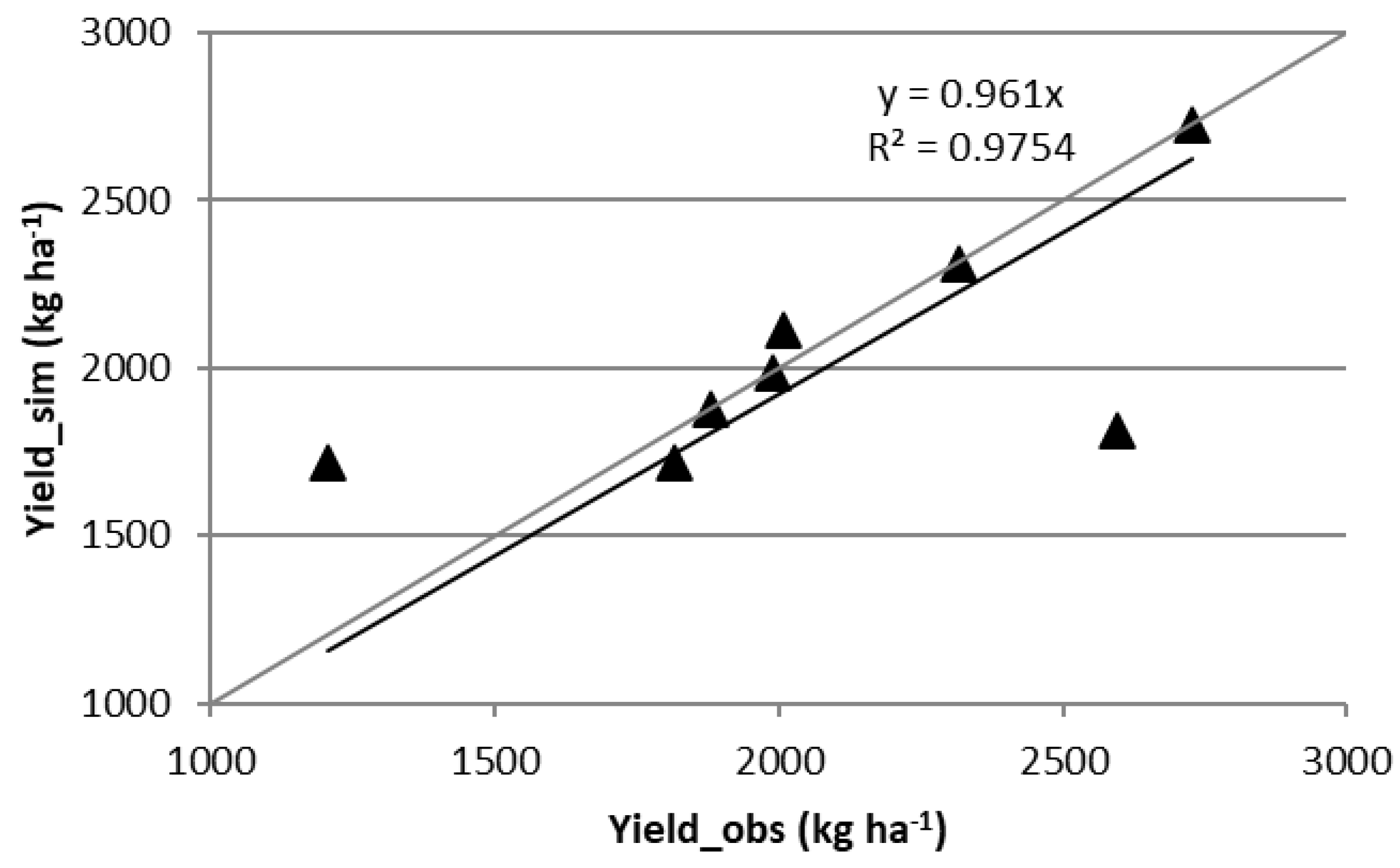
Figure 2.
Productivity in terms of fresh drupes in response to different irrigation management and applied organic fertilization (CTR, a; BCH, b; CMP, c; and DB, d) and their respective mean values.
Figure 2.
Productivity in terms of fresh drupes in response to different irrigation management and applied organic fertilization (CTR, a; BCH, b; CMP, c; and DB, d) and their respective mean values.
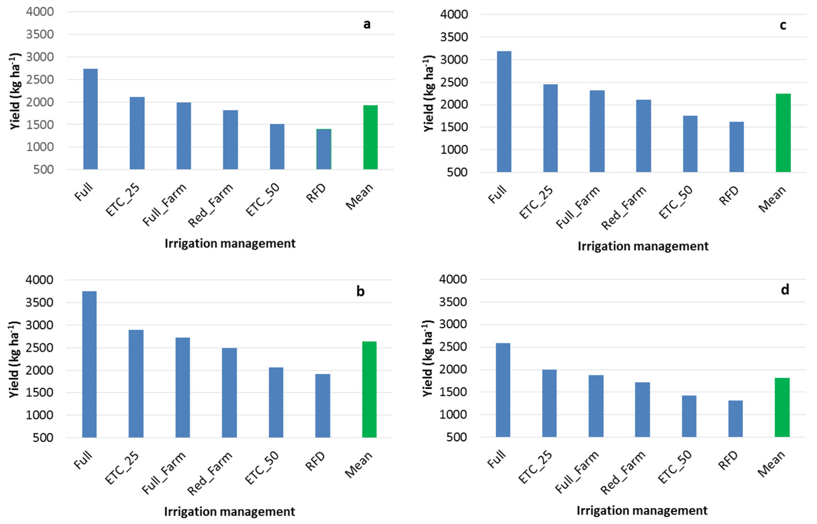
Figure 3.
Increases in the productivity of olive plants in response to increasing seasonal irrigation volumes. The lines indicate the regression between the yield variable and irrigation regime for BCH (solid black line), CMP (solid grey line), CTR (dashed black line), and DB (dashed grey line).
Figure 3.
Increases in the productivity of olive plants in response to increasing seasonal irrigation volumes. The lines indicate the regression between the yield variable and irrigation regime for BCH (solid black line), CMP (solid grey line), CTR (dashed black line), and DB (dashed grey line).
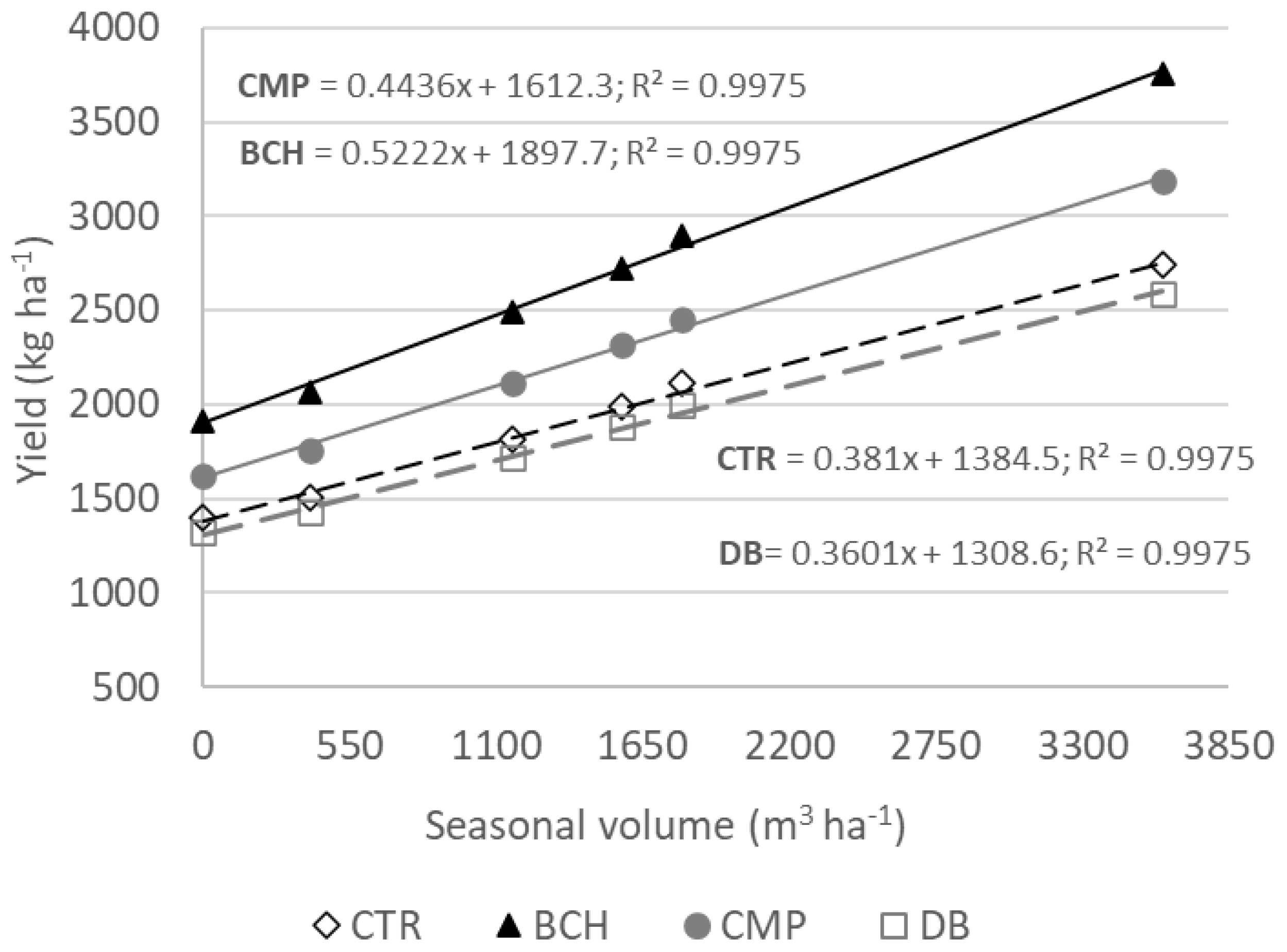
Figure 4.
Total water use (Wusetot) and its various components (green, blue, and grey) under different irrigation regimes and fertilization treatments (CTR, a; BCH, b; CMP, c; and DB, d).
Figure 4.
Total water use (Wusetot) and its various components (green, blue, and grey) under different irrigation regimes and fertilization treatments (CTR, a; BCH, b; CMP, c; and DB, d).
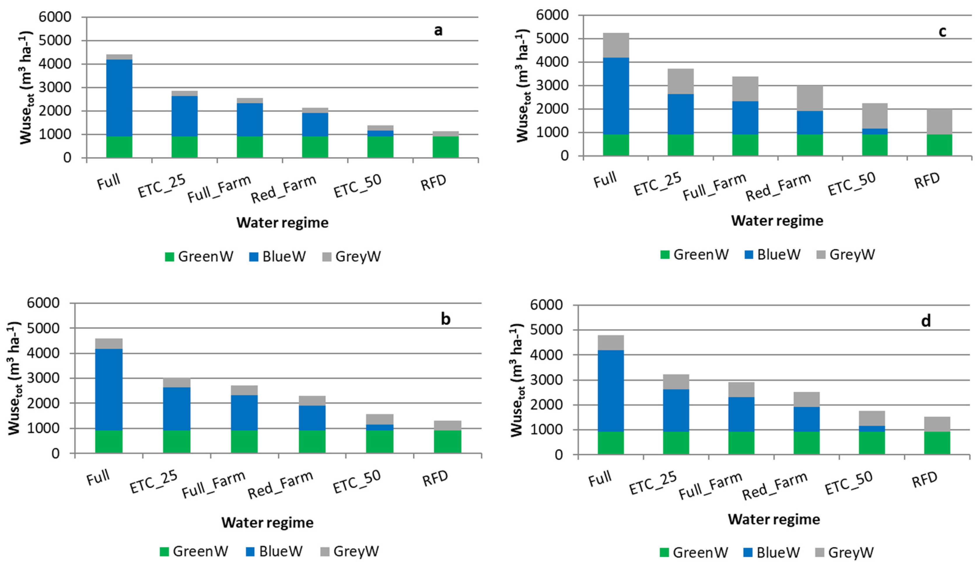
Figure 5.
Water Footprint for fresh drupe production (WFP) under different irrigation regimes and fertilization treatments (CTR, a; BCH, b; CMP, c; and DB, d).
Figure 5.
Water Footprint for fresh drupe production (WFP) under different irrigation regimes and fertilization treatments (CTR, a; BCH, b; CMP, c; and DB, d).
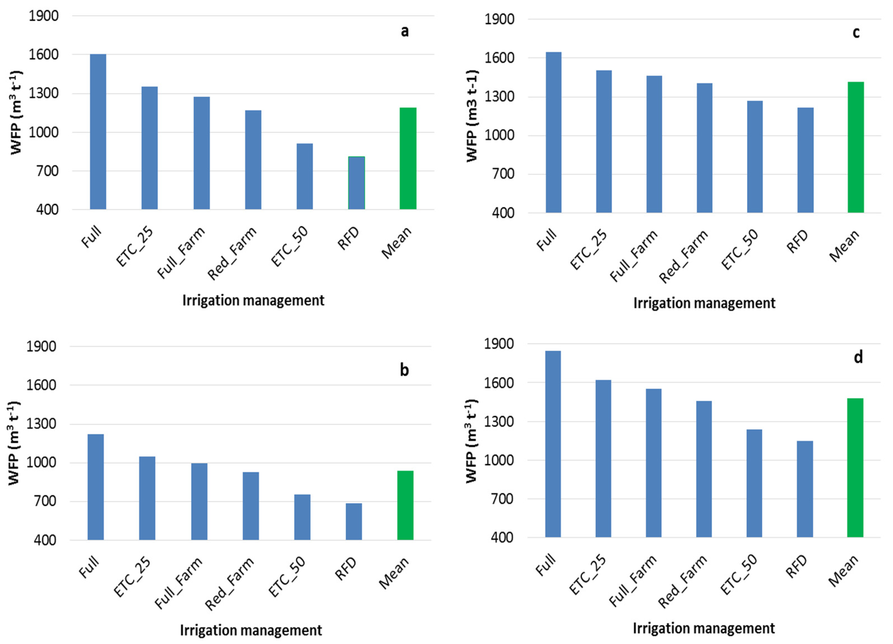
Figure 6.
Production increases in response to irrigation water increments (IRincr), transitioning from one irrigation regime to the next, under different fertilization treatments (CTR, a; BCH, b; CMP, c; and DB, d).
Figure 6.
Production increases in response to irrigation water increments (IRincr), transitioning from one irrigation regime to the next, under different fertilization treatments (CTR, a; BCH, b; CMP, c; and DB, d).
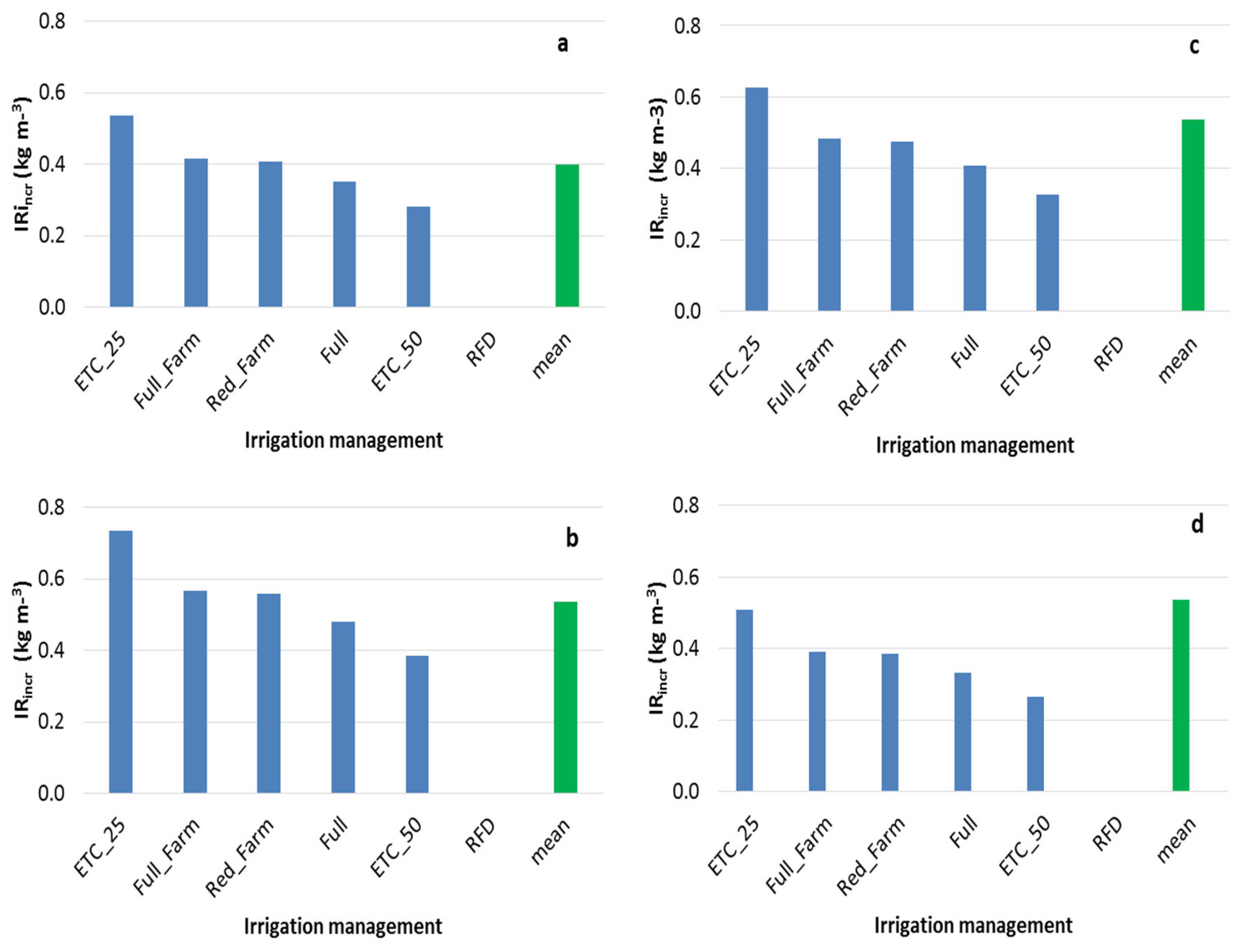
Figure 7.
Increases in terms of Wusetot per unit of production in response to changes in irrigation water (IRincr), transitioning from one irrigation regime to the next under different fertilization treatments (CTR, a; BCH, b; CMP, c; and DB, d).
Figure 7.
Increases in terms of Wusetot per unit of production in response to changes in irrigation water (IRincr), transitioning from one irrigation regime to the next under different fertilization treatments (CTR, a; BCH, b; CMP, c; and DB, d).
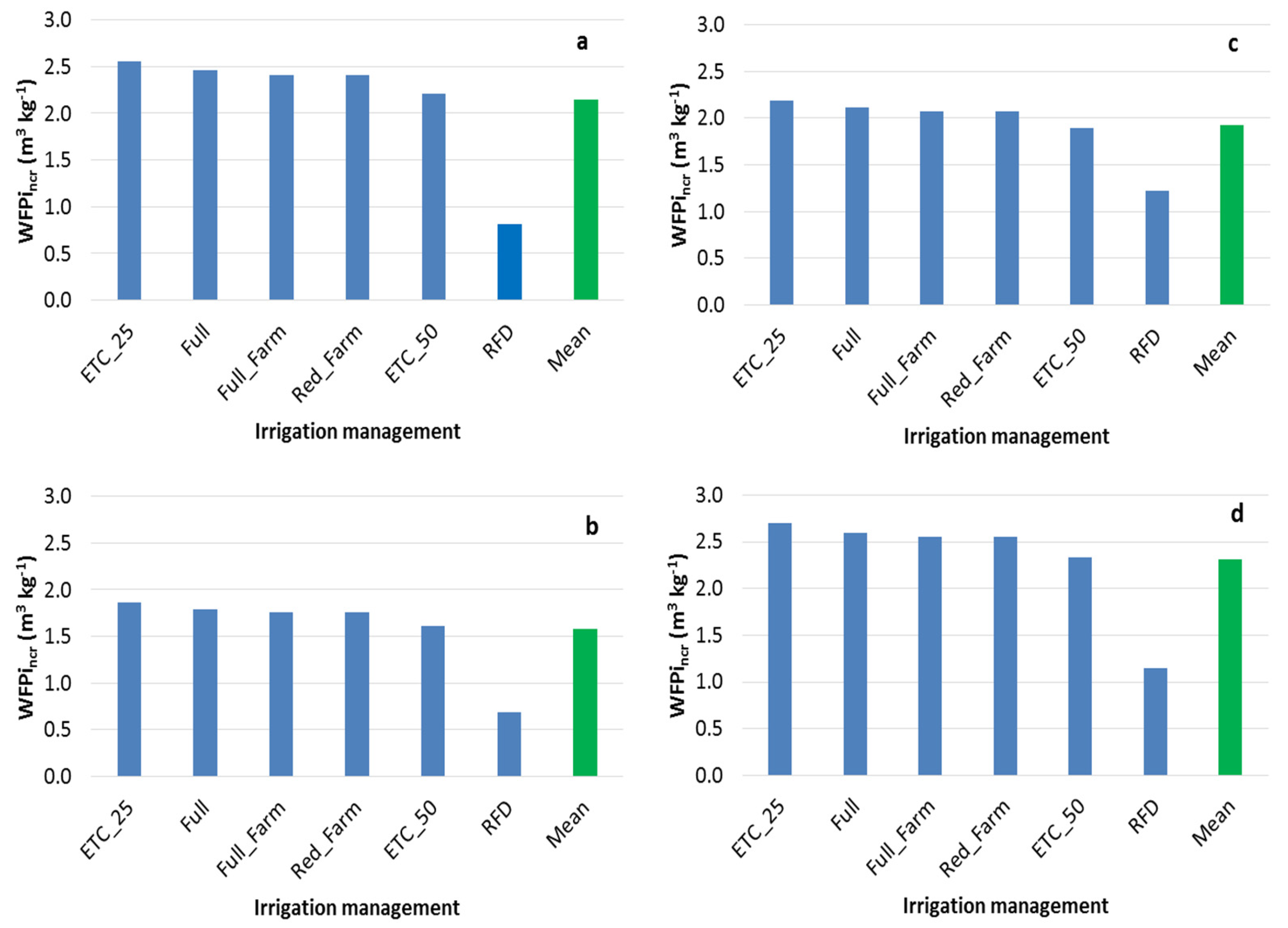
Figure 8.
Cumulative distribution function for yield (a), Wusetot (b), and WFP (c) for all values derived from the combinations of “irrigation management x fertilization treatment”. The dashed lines indicate critical threshold values at the 25th and 75th percentiles, with green marking the favorable threshold and red indicating the unfavorable threshold.
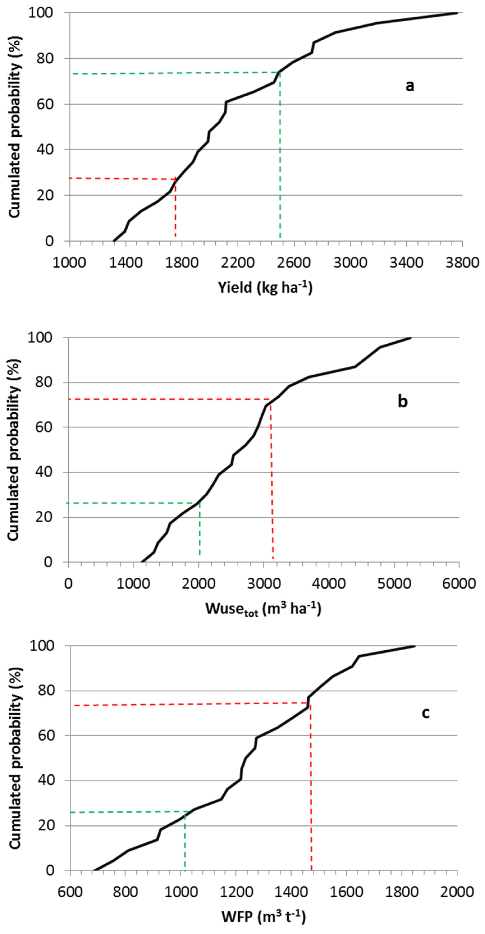
Figure 9.
Cumulative distribution function for WFPincr (a), and IRincr (b) for all values derived from the combinations of “irrigation management x fertilization treatment”. The dashed lines indicate critical threshold values at the 25th and 75th percentiles, with green marking the favorable threshold and red indicating the unfavorable threshold.
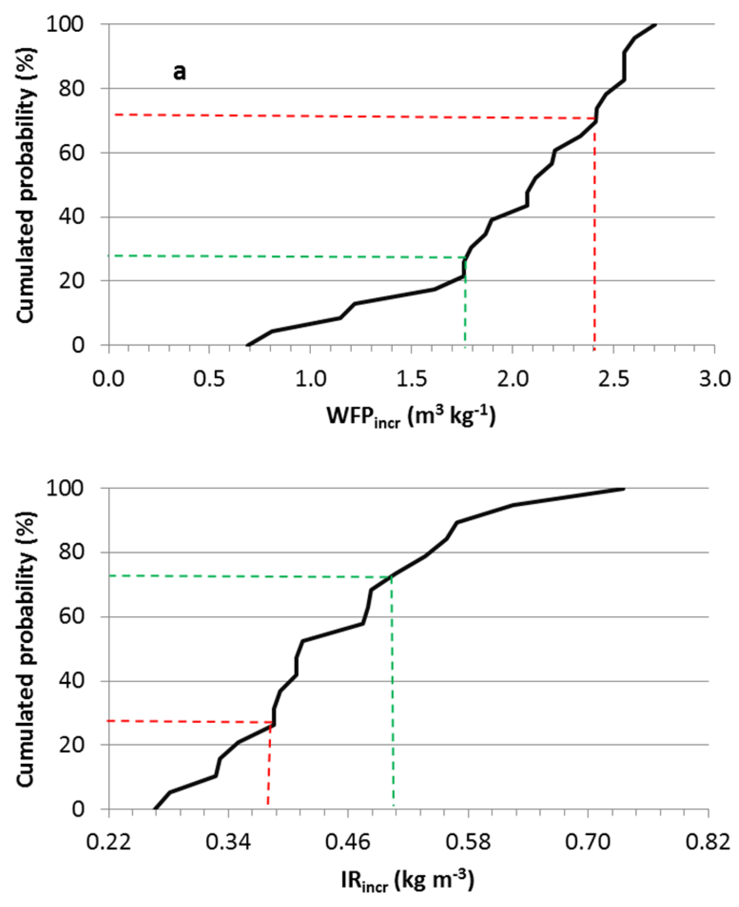
Figure 10.
S-shaped function for assigning a score between 0 (worst) and 1 (best) based on the values of yield (a), Wusetot (b), and WFP (c) in the olive cropping system.
Figure 10.
S-shaped function for assigning a score between 0 (worst) and 1 (best) based on the values of yield (a), Wusetot (b), and WFP (c) in the olive cropping system.
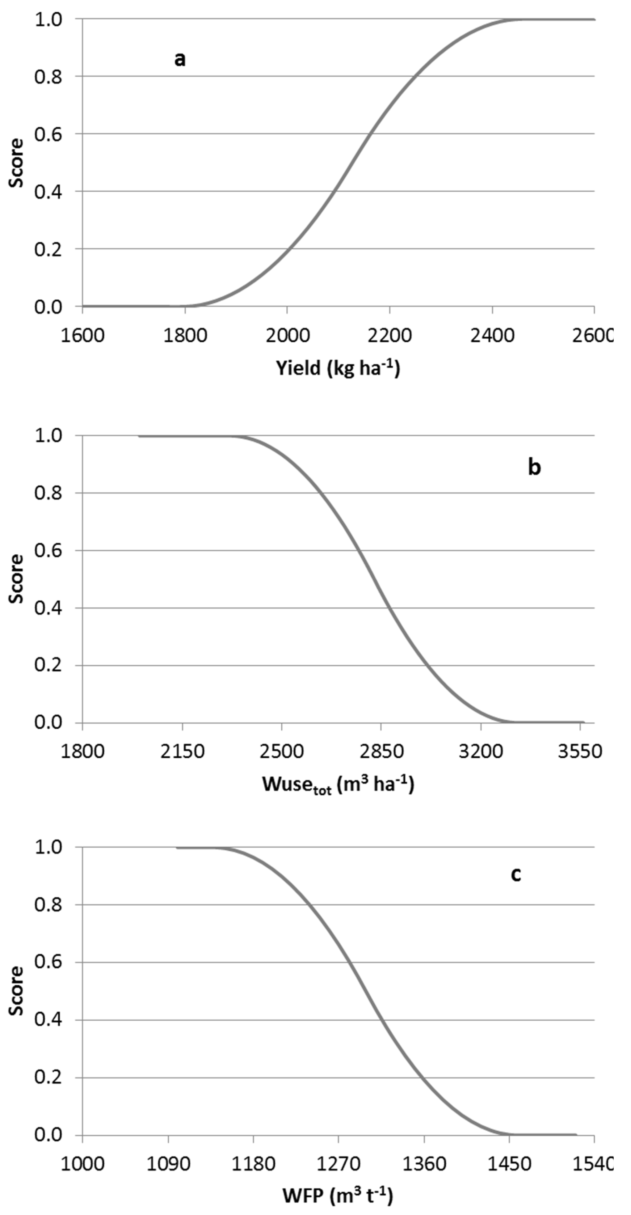
Figure 11.
S-shaped function for assigning a score between 0 (worst) and 1 (best) based on the values of WFPincr (a), IRincr (b) in the olive cropping system.
Figure 11.
S-shaped function for assigning a score between 0 (worst) and 1 (best) based on the values of WFPincr (a), IRincr (b) in the olive cropping system.
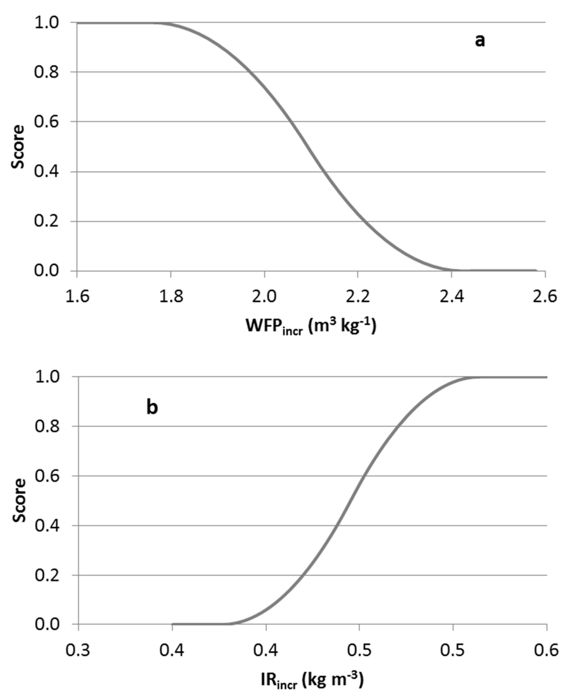
Figure 12.
Aggregated scores (Inaggr) for each “irrigation management x fertilization treatment” combination are derived from the sum of individual scores for each variable investigated within the cropping system. Lower values correspond to poorer overall evaluations (0 being the worst value), while higher values (5 being the maximum achievable value) indicate better performance.
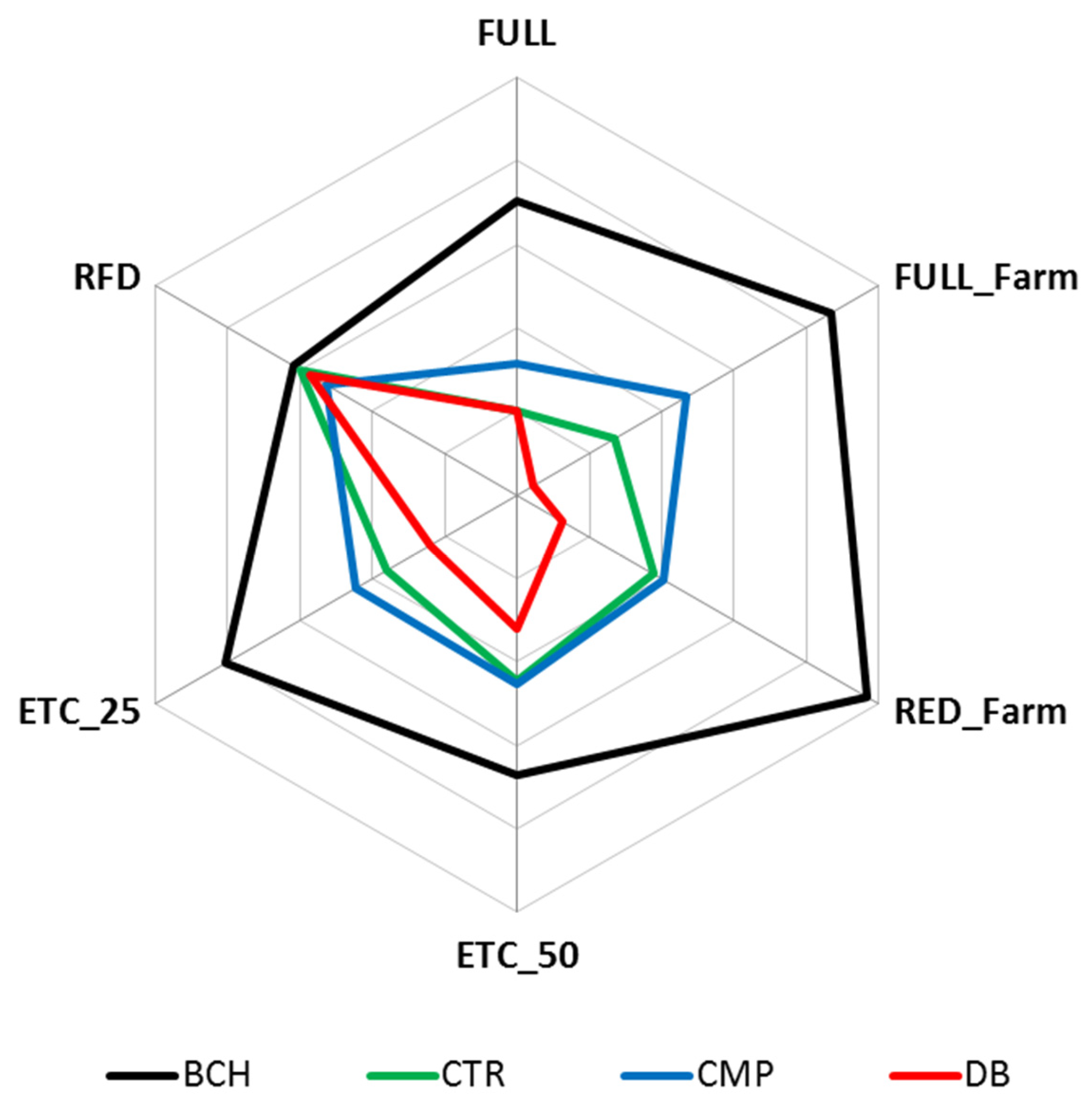

Table 1.
Main chemical properties of compost (CMP) and biochar (BCH).
| Compost | Biochar | |
|---|---|---|
| Moisture (g 100g-1) | 50 | 77 |
| pH | 8.00 | 9.60 |
| Electrical conductivity (dS m-1) | 2.20 | 0.46 |
| Total Organic Carbon (g kg-1 d.m.) | 200 | 882 |
| Nitrogen (g kg-1 d.m.) | 8.00 | 3.00 |
Table 2.
Calibrated parameters for olive cultivation used in CropWat.
| Stage | *Kc | Days | Rootind depth | *Critical depletion (p) | *Yield response factor (f) | Crop height |
|---|---|---|---|---|---|---|
| m | m | |||||
| Initial | 0.65 | 30 | 0.90 | 0.65 | 1.00 | 3.00 |
| Development | - | 80 | - | - | 1.00 | - |
| Mid-season | 0.70 | 55 | 1.50 | 0.65 | 1.00 | - |
| Late season | 0.60 | 80 | - | 0.65 | 1.00 | - |
*Kc = crop coefficient; p = critical soil moisture level where first drought stress occurs; f= relative yield decrease to relative evapotranspiration deficit.
Table 3.
ANOVA summary for the linear regression model (with intercept set to zero) comparing observed and simulated yield by CropWat for the Full_Farm and RED_Farm treatments.
Table 3.
ANOVA summary for the linear regression model (with intercept set to zero) comparing observed and simulated yield by CropWat for the Full_Farm and RED_Farm treatments.
| Source | gdl | Sum of Square | Mean Square | F statistic | p-value |
|---|---|---|---|---|---|
| Regression | 1 | 3.31*10^7 | 3.31*10^7 | 277.07 | <0.001 |
| Residual | 7 | 8.34*10^5 | 11.94*10^4 | ||
| Total | 8 | 3.39*10^7 |
Table 4.
Seasonal water supply, number of irrigations, and water consumed by the cropping system in response to the applied irrigation regime.
Table 4.
Seasonal water supply, number of irrigations, and water consumed by the cropping system in response to the applied irrigation regime.
| Management | *ETp | Seasonal volume | Irrigation | *ETc_act | ETC_act/ETp |
|---|---|---|---|---|---|
| mm | mm | n° | mm | ||
| Full | 601 | 360 | 18 | 601 | 1 |
| ETC_25 | 601 | 180 | 9 | 463 | 0.77 |
| Full_Farm | 601 | 157 | 8 | 436 | 0.73 |
| RED_Farm | 601 | 116 | 7 | 398 | 0.66 |
| ETC_50 | 601 | 40 | 2 | 331 | 0.55 |
| RFD | 601 | 0 | 0 | 309 | 0.51 |
*ETp = potential evapotranspiration; ETc_act = Actual crop evapotranspiration.
Table 5.
Summary of yield, total water use (Wusetot), water footprint (WFP), incremental water footprint (WFPincr), and incremental irrigation response (IRincr) scores for different fertilization treatments under various irrigation strategies. Scores range from 0 (worst performance) to 1 (best performance).
| Fertilizer | Irrigation | Variable | ||||
|---|---|---|---|---|---|---|
| Yield | Wusetot | WFP | WFPincr | IRincr | ||
| CTR | Full | 1.00 | 0.00 | 0.00 | 0.00 | 0.00 |
| Full_Farm | 0.20 | 0.59 | 0.41 | 0.00 | 0.15 | |
| RED_Farm | 0.02 | 0.96 | 0.81 | 0.00 | 0.10 | |
| ETC_50 | 0.00 | 1.00 | 1.00 | 0.22 | 0.00 | |
| ETC_25 | 0.45 | 0.20 | 0.16 | 0.00 | 1.00 | |
| RFD | 0.00 | 1.00 | 1.00 | 1.00 | ||
| BCH | Full | 1.00 | 0.00 | 0.64 | 1.00 | 0.88 |
| Full_Farm | 1.00 | 0.34 | 1.00 | 1.00 | 1.00 | |
| RED_Farm | 1.00 | 0.84 | 1.00 | 1.00 | 1.00 | |
| ETC_50 | 0.35 | 1.00 | 1.00 | 1.00 | 0.01 | |
| ETC_25 | 1.00 | 0.06 | 1.00 | 0.97 | 1.00 | |
| RFD | 0.09 | 1.00 | 1.00 | 1.00 | ||
| CMP | Full | 1.00 | 0.00 | 0.00 | 0.47 | 0.10 |
| Full_Farm | 0.86 | 0.00 | 0.00 | 0.59 | 0.90 | |
| RED_Farm | 0.46 | 0.10 | 0.05 | 0.59 | 0.83 | |
| ETC_50 | 0.00 | 0.90 | 0.43 | 0.94 | 0.00 | |
| ETC_25 | 0.99 | 0.00 | 0.00 | 0.25 | 1.00 | |
| RFD | 0.00 | 1.00 | 0.65 | 1.00 | ||
| DB | Full | 1.00 | 0.00 | 0.00 | 0.00 | 0.00 |
| Full_Farm | 0.06 | 0.14 | 0.00 | 0.00 | 0.02 | |
| RED_Farm | 0.00 | 0.63 | 0.00 | 0.00 | 0.01 | |
| ETC_50 | 0.00 | 1.00 | 0.58 | 0.03 | 0.00 | |
| ETC_25 | 0.21 | 0.00 | 0.00 | 0.00 | 0.99 | |
| RFD | 0.00 | 1.00 | 0.87 | 1.00 | ||
Disclaimer/Publisher’s Note: The statements, opinions and data contained in all publications are solely those of the individual author(s) and contributor(s) and not of MDPI and/or the editor(s). MDPI and/or the editor(s) disclaim responsibility for any injury to people or property resulting from any ideas, methods, instructions or products referred to in the content. |
© 2024 by the authors. Licensee MDPI, Basel, Switzerland. This article is an open access article distributed under the terms and conditions of the Creative Commons Attribution (CC BY) license (http://creativecommons.org/licenses/by/4.0/).
Copyright: This open access article is published under a Creative Commons CC BY 4.0 license, which permit the free download, distribution, and reuse, provided that the author and preprint are cited in any reuse.


