
Submitted:
21 November 2024
Posted:
26 November 2024
You are already at the latest version
Abstract
Many steel bridges are reaching the end of their service life due to increased traffic loads and outdated design practices. To predict their future condition, a hybrid approach for identifying fatigue-related damage, particularly discrete cracks, is applied to steel bridges with orthotropic decks. This method combines a data-driven selection of potential damage locations with highly detailed, physics-based simulation models using the Static Condensation Reduced Basis Element method (SCRBE). Synthetic data from static load tests, based on real-world loading scenarios, demonstrates the approach’s effectiveness on a steel arch bridge with various damage states. The results show that the method can identify damage using global displacement measurements. However, higher loads are required for practical damage detection due to the small effect of discrete damage on the global load-bearing behaviour. The study highlights the importance of focusing on realistic, localised damage, rather than extensive, fictitious scenarios in all damage identification methods. Incorporating innovative simulation techniques and Structural Health Monitoring can improve predictive maintenance for steel bridges, especially given the challenges of complex damage in large structures.
Keywords:
damage identification
; steel bridges
; discrete cracks
; hybrid approach
; reduced order modelling
; structural health monitoring
; orthotropic steel decks
; predictive maintenance
1. Introduction
Steel bridges with orthotropic decks are essential elements of modern infrastructure. Many of them are currently reaching the end of their service life, especially due to increasing traffic volumes and loads far exceeding those anticipated during their original design. The accelerated deterioration of steel bridges is further exacerbated by outdated design details, poor construction practices, insufficient material quality, and inadequate maintenance Wardhana and Hadipriono 2003. This issue is especially evident in older steel bridges, featuring complex orthotropic steel decks with numerous weld seams and connection points.
The primary causes of damage to steel bridges include corrosion, fatigue, local stress peaks, and repeated plastic deformation. These factors lead to common forms of deterioration such as cracks, fractures, surface corrosion, and instabilities like local buckling. Fatigue cracking is particularly widespread and poses a significant challenge to the longevity of steel bridges Fisher and Roy 2011. These cracks often occur simultaneously in multiple locations, frequently in hard-to-access areas. Therefore, innovative digital methods are essential for damage identification at an early stage as part of a predictive maintenance strategy.
Farrar and Worden (2012) define damage broadly as any change in a system that affects the current or future behaviour of the structure in a way that it is no longer operating in its ideal condition. Identifying damage typically involves comparing a known, initial reference state to an unknown, potentially damaged state Farrar and Worden 2012. The current state of the structure is captured using Structural Health Monitoring (SHM), which provides essential insights its condition. While this paper does not focus specifically on SHM, several studies offer a thorough exploration of its opportunities and challenges in the context of bridges Ko and Ni 2005,Modares and Waksmanski 2013,Peil 2005,Rizzo and Enshaeian 2021. The damage identification process itself is commonly divided into four steps Rytter 1993:
- Detection: a qualitative indication of damage,
- Localisation: the probable location of damage,
- Assessment: the extent of damage,
- Consequence: the evaluation of the structural safety given the damage state.
Comprehensive reviews of various damage identification methods, such as those by An et al. (2019), highlight the diversity of techniques used in bridge engineering. In general, two different approaches can be distinguished.
On one hand, there are purely data-driven methods that rely solely on measurement data, without utilising the mechanical behaviour. For instance, principal component analysis of strain responses has been applied to steel truss bridges for damage detection by Azim and Gül (2021), and convolutional neural networks have been used for automatic damage localisation Parisi et al. 2022. Data-driven techniques are popular due to their low computational demands, but they are generally not suitable for the entire damage identification process. While they are effective at detecting and localising damage, they often struggle to assess its severity or predict future conditions.
On the other hand, there are approaches primarily based on physics-based simulation models. In this context, the FE model update is the most common method Ereiz et al. 2022. Schlune et al. (2009) used static and dynamic measurements to update a FE model of the Svinesund Bridge, a single-arch concrete bridge, through non-linear optimisation, while Teughels and de Roeck (2005) employed damage functions and modal characteristics for updating the beam model of the Z24 highway bridge. Ye et al. (2020) incorporated vibration and load testing data in FE updating of a combined shell and beam model for a multi-girder steel stringer bridge, while Sanayei et al. (2012) used a combination of shell and solid elements for a three-span concrete slab on steel stringer bridge as a case study for non-destructive testing and manual FE updating. Ding et al. (2010) proposed a multi-scale FE update method for a long-span cable-stayed bridge with a steel box girder, using a combination of a global shell model and a detailed local model for a single bridge section.
Physics-based models have the advantage of being well-suited for predicting future conditions. However, they require often complex simulations, which can be particularly time-consuming for large-scale structures.
To overcome the limitations of both approaches, hybrid methods combining physics-based models with data-driven techniques have been rising in popularity. Svendsen et al. (2023) combined FE models with supervised machine learning to detect damage in steel bridges under simulated environmental conditions. Similarly, Rageh et al. (2020) used FE models with machine learning to identify fatigue damage in steel railway bridges. Torzoni et al. (2024) developed a comprehensive Digital Twin concept for infrastructure, focusing on probabilistic graphical models.
A key challenge, however, remains in scaling damage identification methods to real-world structures, where damage and conditions are far more complex Kang et al. 2024,Niederer et al. 2021. Due to the high computational effort required for large-scale structures, simplified models such as beam models are usually employed as physics-based models in FE model updating to capture the global load-bearing behaviour with reasonable accuracy. However, in this case detailed sub-models are required for localised analyses of critical points like connections. Therefore, the proper selection of boundary conditions and loads is crucial to ensure the model’s accuracy. With regard to the automatic derivation of simulation models from geometric models, it would be advantageous to use a single highly detailed model to describe the global load-bearing behavior and local details.
To make these so called high-fidelity models more computationally efficient, physics-based reduced-order models (ROMs) are useful. These models retain essential physical characteristics while reducing complexity, striking a balance between accuracy and computational cost for large-scale structures. The Static Condensation Reduced Basis Element (SCRBE) method Huynh 2014,Huynh et al. 2013a,Huynh et al. 2013b is particularly advantageous in this context. Besides reducing the computational effort, it allows for a direct parameterisation of the structure.
The SCRBE method has been successfully applied in various fields, including unmanned aerial vehicles Kapteyn et al. 2022, wing structure analysis Kim et al. 2024, and offshore wind turbines Zhao et al. 2023. Early applications in steel bridges have also been explored Brenner et al. 2023. Other physics-based ROMs include different component-based approaches, such as those used by Fernandez-Navamuel et al. (2022) and Papadimitriou and Papadioti (2013) for bridges together with FE updating or for lattice structures McBane and Choi 2021. An alternative approach involves the application of the adjoint method Löhner et al. 2024 or the use of data-driven surrogate models Ramancha et al. 2022.
In the context of damage identification for large-scale bridges, two main questions remain unresolved. The first question refers to the damage states investigated. Most studies to date have focused on fictitious damage states, typically involving substantial stiffness reductions. These reductions range from to as much as for entire structural members Azim and Gül 2021,Chou and Ghaboussi 2001,Fernandez-Navamuel et al. 2022,Parisi et al. 2022,Rageh et al. 2020,Viola and Bocchini 2013 or for extensive areas of the structure Ding et al. 2010,Kapteyn et al. 2022,Papadimitriou and Papadioti 2013,Schlune et al. 2009,Torzoni et al. 2024. The issue of identifying real damage has only been explored in cases of severely damaged bolted connections, where a significant number of bolts have been removed from a steel truss bridge Svendsen et al. 2023. To date, the identification of fatigue damage in steel bridges, particularly in the form of discrete cracks, has not been thoroughly investigated.
The second unresolved question concerns the complexity of the structures, particularly with respect to the high number of parameters needed to characterise their current state. Typically, a small number of parameters, usually in single or low double digits, are manually predefined in studies of bridges Azim and Gül 2021,Fernandez-Navamuel et al. 2022,Kapteyn et al. 2022,Papadimitriou and Papadioti 2013,Parisi et al. 2022,Schlune et al. 2009,Torzoni et al. 2024. However, this approach necessitates a high degree of prior knowledge about the damage state or results in only a rough localisation of the damage. For bridges with unknown damage states, the need to identify a larger number of parameters remains a significant issue. This often leads to ill-posed and ill-conditioned optimisation problems, for which existing algorithms are not well-suited.
This paper investigates the identification of realistic fatigue-related damage, particularly discrete cracks, in steel bridges with orthotropic decks. In the initial stage, a data-driven algorithm is used to reduce the number of unknown model parameters. The second stage involves evaluating the mechanical behaviour of the structure using high-fidelity parametric models based on the SCRBE method. Synthetic measurement data from a static load test is employed to assess the potential and challenges of this hybrid approach. Static measurements provide greater sensitivity to local damage compared to natural frequencies and can be accurately captured through simple load tests Chou and Ghaboussi 2001,Viola and Bocchini 2013. Additionally, static responses focus on stiffness properties, thereby eliminating the need to account for mass and damping properties. Given the slow development and progression of damage in the construction industry, real-time monitoring is typically unnecessary. Consequently, regular assessments at selected intervals are sufficient. This study addresses the detection, localisation, and assessment of damage, as well as predictions regarding the structure’s future state.
2. Damage Identification of Steel Bridges
A two-stage hybrid approach is employed for identifying damage on steel bridges. In the first stage, a data-driven algorithm is used for the pre-selection of potential damaged areas, thereby reducing the number of model parameters that need to be calibrated. Damage is detected and roughly localised based on variations in the measurement data. In the second stage, a physics-based simulation model is calibrated using the pre-selected parameters. This model is subsequently employed to evaluate the severity of the damage and to predict future conditions. The following section provides a brief explanation of the method used to create the parametric physics-based reduced-order model, followed by an overview of the damage detection algorithm and a description of the case study.
2.1. Physics-Based Reduced-Order Modelling for Large-Scale Structures
The SCRBE method is used to create the physics-based ROM. Due to the fatigue-related damage, a linear-elastic material behaviour is assumed. The basis for the SCRBE method forms a spatial discretisation via a global FE approximation. This results in the following second-order system of ordinary differential equations, which describe the linear static equilibrium of a structure
where is the stiffness matrix of size , the displacement vector, and the force vector. The stiffness matrix is parameterised by the vector . For complex civil structures, the number of degrees of freedom (DOF) n can be exceedingly large, up to for detailed FE models of large bridges. The SCRBE method uses an offline/online decomposition, so that the number of DOF in the online stage is reduced to a few thousand, significantly speeding up computations once the offline training is completed. Therefore, two core numerical techniques are used, static condensation and the reduced basis method Huynh 2014,Huynh et al. 2013a,Huynh et al. 2013b.
The first step is to partition the full model into subdomains (components) and their interfaces (ports) using static condensation. The system of equations for the original FE approximation (Equation (1)) is reorganised as:
where the subscript c refers to component-internal DOF and p to port DOF. Solving the second set of equations for the internal DOF leads to
Substituting this back into the first set results in the condensed system
Thus, the component-internal DOF can be expressed in terms of the port DOF , yielding a condensed stiffness matrix and load vector
The reduced system, now much smaller , is written as
The application of static condensation presents two challenges:
- Direct computation of matrix inverses in Equation (3) is computationally expensive. To overcome this, the FE solves within each component are replaced by the reduced basis method, significantly improving efficiency.
- The condensed stiffness matrix becomes denser, as each component contributes a dense block based on the port DOF. Hence, ports should ideally have fewer DOF, achievable through a strategic choice of port locations. However, this may be challenging for complex structures. To address this, port reduction is carried out within the SCRBE method, determining a reduced number of DOFs on the ports needed to transfer crucial information between adjacent components while maintaining accuracy Eftang et al. 2012,Eftang and Patera 2013,Eftang and Patera 2014.
The reduced basis method enhances the computational efficiency of FE analyses inside the components by approximating the solution space with a lower-dimensional basis. In the context of the SCRBE method, the reduced basis method builds a reduced approximation of the displacement vector as follows:
where is the reduced basis matrix composed of a set of basis vectors (or modes) that span the solution space, and is the vector of coefficients representing the combination of these basis vectors. In practice, the matrix is constructed during the offline phase of the SCRBE method by sampling the parameter space and computing solutions to the full problem.
The reduced model then substitutes into the original Equation (1), yielding
Multiplying both sides by , the transpose of the reduced basis matrix, gives the reduced system
where
By employing the reduced basis method, the computational process is streamlined, as the number of degrees of freedom is drastically reduced from (the total DOF inside each component) to (the number of chosen reduced DOFs inside each component), with .
This paper employs a commercial implementation of the SCRBE method in the software Akselos 2024 Akselos SA 2024. To ensure that the simulation model can be adapted to the measurement data, each component i is parameterised applying by a stiffness reduction factor to the initial stiffness
A preliminary assessment of the required parameter range is conducted to optimally capture the discrete cracks as realistic damage scenarios investigated here. The results indicate that the values of the parameter can be constrained to the range where a parameter of denotes the undamaged state and a parameter of corresponds to a reduction in stiffness of .
The primary task in applying the SCRBE method is to select the most suitable components to fully use its advantages. In addition to the numerical influences described earlier, the characteristics of the structure and the potential damage locations must also be considered. For instance, it is impractical to divide the entire structure into its main structural elements due to geometric discontinuities and the expected damage locations at the intersections. In this context, detailed investigations into automating the component definition for steel bridges characterised by regular structures have been conducted by Brenner et al. (2024). The definition of the components is based on these investigations and will not be explained in detail here.
2.2. Damage Identification Using a Hybrid Approach
For damage identification, static responses from static load tests are utilised. Consequently, strains and vertical deflections are suitable measured variables. However, using strains in conjunction with the chosen parameterisation of the SCRBE model and potential sensor placements within components is problematic. A crack creates a discontinuity that redirects the stress trajectories within the structure. As a result, the measured strains from neighbouring strain gauges are lower in comparison to the undamaged state due to load redistribution. In contrast, when damage is approximated by a distributed stiffness reduction, as is the case with the selected parameterisation of the components in the SCRBE method, the measured strains increase according to Hooke’s law, . This occurs because no load redistribution takes place, leading to approximately constant stresses.
One possible solution to this issue is to exclude sensors within parameterised components from the analysis Kapteyn et al. 2022. However, this approach is not always feasible due to the unknown location of the damage and the positions of the available sensors. On the other hand, both discrete cracks and distributed stiffness reductions result in local increased vertical displacements. Therefore, deflections are selected as the measured variable for this analysis.
2.2.1. Selection of Damage-Relevant Sensors and Parameters
The first step of the hybrid damage identification approach is a data-driven algorithm designed to detect and localise changes in the measurement data and transfer potential damage locations to the physics-based model. This algorithm can be applied repeatedly and efficiently to a large number of measurements or measurement time series. The algorithm compares two structural conditions. The first state, denoted as state , is the initial state where the damage condition and all parameters are known. This baseline is crucial for all damage detection algorithms Farrar and Worden 2012. The second state, denoted as state , is a new, unknown state that might be damaged. In this study, it is assumed that all changes in displacement result from damages, so no filtering of environmental effects is applied.
If damage occurs in the form of a discrete crack, it is assumed that the deflection locally increases compared to the undamaged state. However, given the size of the entire structure, the influence of the crack on global structural behaviour is quite limited. Therefore, it is assumed that the measurement point closest to the damage will experience the greatest increase in deflection. As the distance from the damage location increases, the changes in the sensor readings diminish. Consequently, a potential crack can be identified as a positive peak in the differences in deflection between the damaged and undamaged states. This relationship is formulated mathematically in Algorithm 1.
Initially, all sensors in regions of potential damage are identified. These sensors are then mapped to the parameters of the physics-based model based on their positions. If a measurement point is located within a parameterised component, that parameter is selected. If a clear assignment is not possible, all neighbouring parameters are chosen instead.
| Algorithm 1 Parameter selection based on displacement measurement difference |
|
Two hyperparameters are included in the sensor selection process to enhance the robustness of the algorithm and diminish sensitivity to measurement noise. The first is the absolute threshold . This threshold excludes sensors with reduced deflections after damage and those with only slight increases in deflection. The second hyperparameter is the minimum value for the gradient . This value checks whether the gradient of the deflection difference is sufficiently large, effectively serving as a threshold for damage detection. Here, a threshold value of is set and an absolute threshold value of is selected. Due to the subsequent calibration of the physics-based model, more potential damaged parameters should be selected to detect damage events as early as possible. All undamaged parameters will be set to nearly zero by the optimisation algorithm if suitable accuracy is used.
2.2.2. Update of Model Parameters of the Simulation Model
In the second step, the potential damaged parameters selected by the data-driven algorithm are calibrated within the physics-based model using the measurement data from the damaged state. This process of calibration and updating parameters can be regarded as an inverse problem Bonnet and Constantinescu 2005,Friswell 2007. The objective in damage identification inverse problems is to estimate the stiffness reduction parameters from sensor measurements . The relationship between the measurements and the parameters is modelled with a forward model , as follows:
where represents measurement noise or model errors. The forward model, in this case the SCRBE model, predicts the sensor measurements denoted by . The inverse problem of finding the optimal set of stiffness reduction parameters is typically formulated as the minimisation of an objective function :
The minimisation of can be carried out using any minimisation algorithm. Any error measure can be utilised for the objective function. Here, the residual sum of squares is employed as the objective function. It is defined as:
for m measurement points, where are the observed data points and are the predicted values from the SCRBE model. The minimisation in Equation (15) is performed using a standard gradient-based L-BFGS-B algorithm Byrd et al. 1995,Zhu et al. 1997 implemented in the Python package scipy.optimize Virtanen et al. 2020. The optimisation is stopped when the difference in every parameter from the last iteration to the current iteration is less than . For the selected parameter range, this corresponds to a parameter accuracy of .
3. Case Study: A Large-Scale Tied Arch Bridge
The proposed methodology is tested in a real-world scenario using synthetic measurement data from realistic damage states. The examined structure is a large-scale tied arch bridge, as shown in Figure 1.
Constructed in 1981, the bridge spans and accommodates two vehicle lanes and a footpath within a total width of . It crosses an inland waterway canal, which is about wide at this point. The bridge comprises two I-shaped stiffening girders approximately in height on both sides. Traffic loads are transferred to the main load-bearing system via an orthotropic steel deck, which is stiffened in the longitudinal direction primarily by trapezoidal hollow stiffeners. Cross girders are arranged in a regular grid with a spacing of . The hangers, designed as I-sections, connect to the stiffening girders at the height of every second cross girder, spaced apart. Consequently, there are twelve hangers on each side of the bridge. The arch itself is designed as a two-cell hollow section.
The bridge exhibits various damages, particularly at the welds connecting the webs of the I-shaped hangers to the upper flanges of the stiffening girders (see Figure 2). These cracks are predominantly located on the roadway side of the bridge, limiting the major damage locations to these twelve hangers. The crack lengths vary, extending up to at each corner of the web. To assess the structural integrity of the bridge, a load test was conducted in 2021 using a weighted truck (see Figure 3), focusing on five load positions in each vehicle lane.
Based on existing construction drawings, the as-designed geometry of the bridge is modelled. As the bridge has no symmetries in longitudinal or transverse direction, a complete model of the entire structure is required. The geometric model is highly detailed and incorporates both the cross slope of the bridge and its longitudinal superelevation. The structure is primarily modelled using the middle surfaces of the metal sheets. As no damage is expected on the upper part of the hangers or the arches, simpler line representations are used for these parts. The geometric model is depicted in Figure 4.
Due to the absence of an extensive monitoring system on the bridge, synthetic damage states and sensors are employed, based on the existing damage shown in Figure 2. Among the twelve hanger connections on the roadway side, the connections of hanger 2, 4, and 7 are chosen as potential damage locations (see Figure 4). Two potential damage states (crack lengths of or on each corner of the web of the hanger) are investigated. For the hanger’s normal stiffness, cracks correspond to a reduction, while cracks correspond to a reduction in normal stiffness. In total, ten different combinations of one or more cracks with different severities are examined. The damage states are summarised in Table 1.
Since the damages investigated here are located exclusively in the first half of the bridge, three load positions from the static load tests as marked in Figure 4 are used for damage identification in this case study. The loads of the weighted truck are applied via the wheel weights as surface loads for the respective wheel contact areas, rendering the application as realistic as possible. For the proposed damage identification approach, it is assumed that the load test is repeated on a regular basis.
The synthetic monitoring system is designed to identify damages at the hanger connections on the roadway side, based on previous investigations of the real structure. It is assumed that vertical deflection measurements are taken every along the bottom flange of the stiffening girder on the roadside of the bridge (see Figure 4). This results in a total of 25 measurement locations. Since the measurements are not carried out continuously under traffic load but only at regular intervals in combination with the static load tests, contactless displacement measurements are particularly suitable. For instance, laser scanners or total stations can be used for this purpose Moser et al. 2024.
Based on the geometric model, a FE mesh is generated using shell and beam elements, consisting of approximately elements. Due to the efficient SCRBE method, no simplified truss model is necessary for repeated model evaluation during the parameter calibration process. Based on previous investigations on numerics and methodology Brenner et al. 2024, the structure is divided into 81 components, offering a good balance between accuracy and computational effort, comparable to a standard truss model in terms of parameter complexity. The component model is shown in Figure 5. Based on the assumed damage locations and the defined measurement positions, the twelve hanger connections on the roadway side were selected from all 81 possible parameters for parameter identification. The parameterised components are highlighted in Figure 5.
4. Results
As shown in Figure 6, the global deformation behaviour of the bridge is effectively described by the existing measurement locations. The three investigated load positions lead to varying deformations, which can be utilised to identify different types of damage in the first half of the bridge.
In the following, the results of the data-driven algorithm for single, double, and triple damages are detailed. Afterwards, the identified parameters of the physics-based model are presented for selected damage states. The final section addresses the prediction of additional damage using a previously calibrated model.
4.1. Comparison of the Undamaged and Damaged Model States
To obtain the synthetic measurement data of the damaged structure, the corresponding components of the SCRBE model are replaced by components in which the damage has been modelled as shown in Figure 4. The vertical deflections of the undamaged and damaged conditions are then compared for all damage states (1 to 10, see Table 1) and load cases (1 to 3, see Figure 4).
First, the effects of a single damage on hanger 4 or 7 with two different intensities are examined (damage states 1 to 4). The top row of Figure 7 shows the displacement alterations between the undamaged and damaged structures at hanger 7. As expected, the displacement alteration is particularly noticeable for load case 3, as the load is positioned near the damaged hanger. The other two load cases are only slightly affected. Comparing the two damage intensities in the left and right diagram reveals that the displacements differences are non-linearly dependent on the crack lengths. Doubling the crack length from to results in only a slight increase in deflection.
The bottom row of Figure 7 indicates that damage to hanger 4 is more challenging to detect. Due to its position near the turning point of the deflections, detection is most likely to be feasible with the load cases 1 and 2 near the edge of bridge. Unlike for hanger 7, not only the displacements due to the immediately adjacent load position are influenced (here load case 3). As the crack length increases to , the differences become more significant. In most cases, only the parameters with the actual damage are identified as possible parameters via the algorithm. Due to the low threshold value for the gradient, two additional possible damage locations are selected for a crack on hanger 7.
The same effect can be observed in Figure 8 when examining a second damage alongside the crack on hanger 7. As previously mentioned for the single damage, additional damage to hanger 4 is also difficult to detect (damage states 5 and 6). In contrast, damage to hanger 2 with the immediately adjacent load case 1 can be easily identified through changes in vertical displacements (damage states 7 and 8). In all cases, the data-driven algorithm primarily identifies the damaged parameters. However, for the additional cracks on hangers 4 and 2, one additional parameter is identified as possibly damaged in each case.
If all three types of damage occur simultaneously, the aforementioned observations remain consistent as it can be seen in Figure 9. It is also noteworthy that the different types of damage only have a minor influence on one another due to the different load cases. Consequently, the changes in displacements remain nearly unchanged to the previous damages state with single or double damages.
4.2. Identification of Optimal Physics-Based Models
Two damage states with varying intensities, involving one, two, and three cracks respectively, are selected to calibrate the parameters using the parametric ROM. For a single damage on hanger 7 (damage states 1 and 2), only parameter 7 is adjusted for both crack lengths of and . The two incorrectly selected parameters 4 and 5 for a crack are set to nearly zero by the optimisation process. As previously observed in the displacement differences (see Figure 7), it is not possible to differentiate between the two damage intensities for the given damage. The nearly identical displacement changes also lead to similar stiffness reduction parameters, even for different crack lengths.
As expected, a second damage of or on hanger 4, combined with a damage on hanger 7 (damage states 5 and 6), results in very similar stiffness reduction values for parameter 7 compared to the earlier single crack. For parameter 4, the value remains nearly identical for both crack lengths, although it is about half the size of that for parameter 7, despite the same damage intensity. All other undamaged parameters are also significantly reduced by the optimisation and are negligible in comparison.
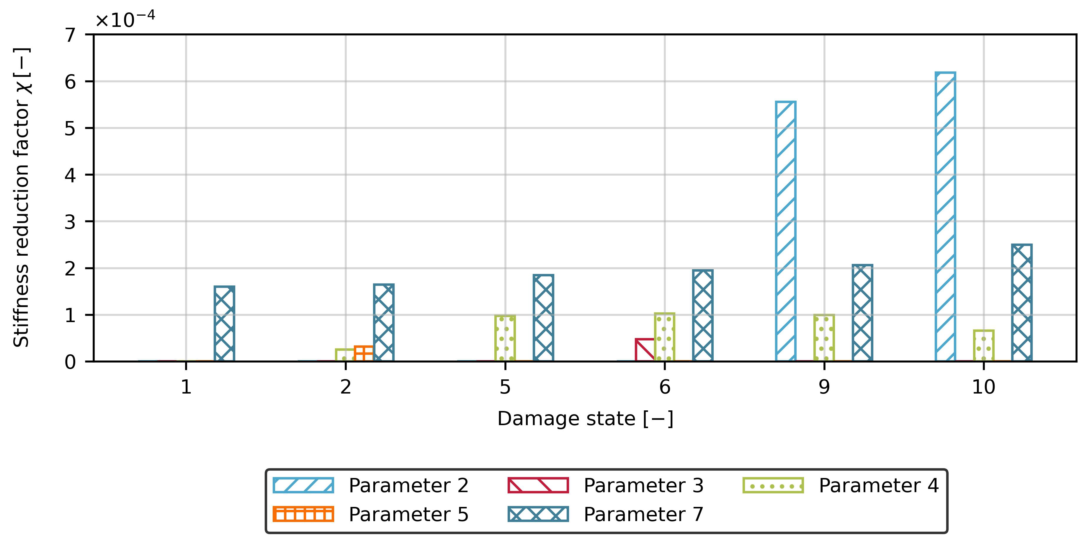
The results for a triple damage scenario, with a or crack on hanger 2 and cracks on hangers 4 and 7, align with the previous findings. Parameters 4 and 7 remain almost unchanged, similar to the damage itself. As before, the resulting stiffness reduction coefficients for hanger 2 differ significantly from those of parameters 4 and 7, despite the same damage intensity. This leads to a parameter value that is approximately three times larger than parameter 7 and six times larger than parameter 6, regardless of the crack length.
Figure 10.
Calibrated parameters for one, two and three simultaneous damages
4.3. Prognosis of Proceeding Damage
To test the predictive ability of the calibrated model, it is assumed that there is a crack on hanger 7 (damage state 2). The parametric ROM is then calibrated as before, resulting in a value of for parameter 7. This model serves as the new baseline for future damage identification. The deflection differences can thereafter be recalculated for damage states 5 to 10, allowing the hybrid approach to be applied again. Figure 11 presents the new displacement differences for a single additional damage at hanger 4 (damage states 5 and 6) or at hanger 2 (damage states 7 and 8).
Compared to Figure 8, it is evident that the peak at hanger 7 (at ) has nearly disappeared, while the other damages can still be easily detected. Due to the low threshold value for the gradient within the data-driven algorithm, parameter 7 is still identified as damaged. However, with higher threshold values, only the new damages would be detected. At this point, a new calibration of the model is not necessary, as the same values would result, as shown in Figure 10. Even if two additional cracks would occur simultaneously (damage states 9 and 10), detection based on the new baseline model results remains possible, as demonstrated in Figure 12.
5. Discussion
For damage identification using the hybrid approach, it is assumed that the initial damage state is known which is always required Farrar and Worden 2012. While this holds true in combination with synthetic measurement data, there tend to be significant deviations for real structures, particularly concerning material properties, geometry, loading and measurements. Theoretically, an initial calibration of the parametric ROM can be performed using all model parameters. The parameters identified in this case may not represent the current damage state but rather include all uncertainties. This model then serves as a baseline for detecting potential damage.
Furthermore, the proposed approach assumes that the same static load tests are conducted for the initial condition and all subsequent damaged conditions. Therefore, load tests must be performed at regular intervals, such as during structural inspections, which necessitates closing the bridge to traffic. Although the load positions were recorded with high precision during the static load test, replicating the exact load distribution across the individual wheels in future tests can be challenging. The influence of possible variations in the wheel loads or positions on the result of the damage identification and the robustness of the hybrid approach still need to be investigated.
Additionally, different environmental conditions, such as temperature and wind, must also be considered. As an alternative, the influence of these environmental conditions on measurement data can be filtered out Deraemaeker and Worden 2018 or considered as additional uncertainties in a Bayesian update approach Ramancha et al. 2022. In any case, a certain level of prior knowledge about potential damage locations and possible damage intensities is essential to determine all necessary load positions for damage identification.
Unlike the current state of research, this paper examines realistic, discrete damages together with actual loads from a weighted truck rather than fictitious, extensive damages to entire structural members or regions. For all investigated damage scenarios, the differences in global deflection are less than . Given a possible sub-millimetre accuracy of contactless displacement measurements Moser et al. 2024, identifying the damage becomes impossible when considering measurement noise. To reliably detect these small damages, a greater load than that provided by a single truck weighing is required.
Additionally, it is important to consider that damage at different locations can have diverse effects on the global load-bearing behaviour and safety of the structure. As a result, each type of damage must be reviewed individually. A conventional assessment of the structural integrity of the investigated bridge, based on Eurocode standards, indicated that the existing damage is not critical and has minimal impact on the global structural behaviour. This finding is consistent with the observed results and the expected small changes in displacement. In contrast, more critical damage to main load-bearing elements, such as the stiffening girders, has a more significant effect on deflections and can therefore be identified more easily.
The limited impact of the examined realistic damage on the global load-bearing behaviour also affects the accuracy of the identified parameters. It is evident that the different damage intensities cannot be represented by the proposed approach, as the differences in deflections are minimal. One possible cause could be that an initial crack of induces a load redistribution within the model, which can be detected through deformation differences. However, the larger crack length of is still considerably smaller than the dimensions of the hanger’s web and therefore has no significantly greater impact on the measurement data. Increasing the load would likely accentuate these differences, potentially leading to clearer outcomes during parameter optimisation.
The results in Figure 10 indicate that a direct assessment of damage severity based solely on parameter values is not feasible because the same crack lengths at different locations in the structure yield different parameter values. One reason for this variation could be the complex shell model, combined with the existing measurement positions, which makes the system highly statically indeterminate. Depending on a component’s location within the structure, a parameter may have a greater or lesser influence on the measured deflections. For example, parameter 2 is situated near the edge of the bridge, where the compact arch base provides significant stiffness. Consequently, very high parameter values are obtained during optimisation.
In contrast, parameter 4, located approximately at the quarter point, has a higher effect on the global load-bearing behaviour, resulting in smaller stiffness reduction values for the same level of damage. Parameter 7, which is positioned roughly in the middle of the field, exhibits an influence that lies between the two previously described cases. This parameter primarily affects the surrounding sensors but has less impact on load transfer to either end of the bridge, unlike parameter 4. Additionally, the size of the component must be considered, especially due to the longer hanger connections extending towards the centre of the bridge.
6. Conclusions
The proposed hybrid approach to damage identification, comprising a data-driven selection of potential damage locations followed by the calibration of stiffness reduction parameters in a physics-based model, proves highly effective for large-scale structures like bridges. The data-driven method allows for repeated localisation of probable damages, significantly reducing the computational effort of subsequent model calibration. Consequently, the optimisation problem for identifying parameters in the physics-based model is notably simplified.
The use of a high-fidelity simulation model is enabled through reduced order modelling. This approach allows for accurate predictions of the mechanical behaviour while requiring less computational effort for repeated model evaluations. The Static Condensation Reduced Basis Element method, utilised in this study, is especially advantageous as a simulation model due to its component structure and natural accommodation of parameterisation. This ensures that, with minimal computational cost, a robust and detailed simulation model is available for predicting future states.
The investigation of realistic fatigue damage in the form of discrete cracks reveals significant challenges in identifying such damage. These are not adequately addressed in the current state of research. The damage states examined in the literature to this point, characterised by large areal stiffness reductions of or more, do not reflect realistic scenarios. Consequently, the methods developed cannot be effectively applied in practice. In the future, all methods of damage identification should be assessed based on their ability to identify real, typical structural damage. The hybrid approach presented here is generally capable of identifying realistic damage when appropriate loading is applied.
In future, the application of this method to real measurement data will be investigated, alongside exploring how traffic-induced deflections can contribute to damage identification. Moreover, by incorporating automated action recommendations, the model has the potential to evolve into a powerful Digital Twin, enhancing predictive maintenance capabilities within the framework of Building Information Modelling.
Acknowledgments
The research presented in this paper is being conducted within the project “Digital twin as an intermediary between in-situ damage detection and global structural analysis”. The project is part of the Priority Programme SPP 2388 "Hundred plus - Extending the Lifetime of Complex Engineering Structures through Intelligent Digitalization", funded by the Deutsche Forschungsgemeinschaft (DFG, German Research Foundation) - project number 501823987.
Conflicts of Interest
The authors declare no conflict of interest.
References
- Akselos SA. 2024. Akselos Modeler (Version 2024.4.1.1) [Computer Software].
- An, Yonghui, Eleni Chatzi, Sung-Han Sim, Simon Laflamme, Bartlomiej Blachowski, and Jinping Ou. 2019. Recent progress and future trends on damage identification methods for bridge structures. Structural Control and Health Monitoring 26(10). [CrossRef]
- Azim, Md Riasat and Mustafa Gül. 2021. Data-driven damage identification technique for steel truss railroad bridges utilizing principal component analysis of strain response. Structure and Infrastructure Engineering 17(8), 1019–1035. [CrossRef]
- Bonnet, Marc and Andrei Constantinescu. 2005. Inverse problems in elasticity. Inverse Problems 21(2), R1–R50. [CrossRef]
- Brenner, Christoph, Klaus Thiele, and Julian Unglaub. 2023. A reduced-order digital twin for structural health monitoring of steel bridges. In S. Farhangdoust, A. Guemes, and F.-K. Chang (Eds.), Proceedings of the 14th International Workshop on Structural Health Monitoring. DEStech Publications, Inc. [CrossRef]
- Brenner, Christoph, Klaus Thiele, and Julian Unglaub. 2024. Constraints of local stiffness adaption for reduced-order models of large-scale steel bridges. e-Journal of Nondestructive Testing 29(7). [CrossRef]
- Byrd, Richard H., Peihuang Lu, Jorge Nocedal, and Ciyou Zhu. 1995. A limited memory algorithm for bound constrained optimization. SIAM Journal on Scientific Computing 16(5), 1190–1208. [CrossRef]
- Chou, Jung-Huai and Jamshid Ghaboussi. 2001. Genetic algorithm in structural damage detection. Computers & Structures 79(14), 1335–1353. [CrossRef]
- Deraemaeker, A. and K. Worden. 2018. A comparison of linear approaches to filter out environmental effects in structural health monitoring. Mechanical Systems and Signal Processing 105, 1–15. [CrossRef]
- Ding, YouLiang, AiQun Li, DongSheng Du, and Tao Liu. 2010. Multi-scale damage analysis for a steel box girder of a long-span cable-stayed bridge. Structure and Infrastructure Engineering 6(6), 725–739. [CrossRef]
- Eftang, J. L., D. B.P. Huynh, D. J. Knezevic, E. M. Ronquist, and A. T. Patera. 2012. Adaptive port reduction in static condensation. IFAC Proceedings Volumes 45(2), 695–699. [CrossRef]
- Eftang, Jens L. and Anthony T. Patera. 2013. Port reduction in parametrized component static condensation: approximation and a posteriori error estimation. International Journal for Numerical Methods in Engineering 96(5), 269–302. [CrossRef]
- Eftang, Jens L. and Anthony T. Patera. 2014. A port-reduced static condensation reduced basis element method for large component-synthesized structures: approximation and a posteriori error estimation. Advanced Modeling and Simulation in Engineering Sciences 1(1), 3. [CrossRef]
- Ereiz, Suzana, Ivan Duvnjak, and Javier Fernando Jiménez-Alonso. 2022. Review of finite element model updating methods for structural applications. Structures 41, 684–723. [CrossRef]
- Farrar, Charles. R. and Keith Worden. 2012. Structural health monitoring: A machine learning perspective. Chichester, West Sussex, U.K and Hoboken, N.J: Wiley. [CrossRef]
- Fernandez-Navamuel, Ana, Diego Zamora-Sánchez, Ángel J. Omella, David Pardo, David Garcia-Sanchez, and Filipe Magalhães. 2022. Supervised deep learning with finite element simulations for damage identification in bridges. Engineering Structures 257, 114016. [CrossRef]
- Fisher, J. W. and S. Roy. 2011. Fatigue of steel bridge infrastructure. Structure and Infrastructure Engineering 7(7-8), 457–475. [CrossRef]
- Friswell, Michael I. 2007. Damage identification using inverse methods. Philosophical transactions. Series A, Mathematical, physical, and engineering sciences 365(1851), 393–410. [CrossRef]
- Huynh, D. B. P. 2014. A static condensation reduced basis element approximation: application to three-dimensional acoustic muffler analysis. International Journal of Computational Methods 11(03), 1343010. [CrossRef]
- Huynh, D. B. P., D. J. Knezevic, and A. T. Patera. 2013a. A static condensation reduced basis element method : approximation and a posteriori error estimation. ESAIM: Mathematical Modelling and Numerical Analysis 47(1), 213–251. [CrossRef]
- Huynh, D. B. P., D. J. Knezevic, and A. T. Patera. 2013b. A static condensation reduced basis element method: Complex problems. Computer Methods in Applied Mechanics and Engineering 259, 197–216. [CrossRef]
- Kang, Chongjie, Jan-Hauke Bartels, Chris Voigt, and Steffen Marx. 2024. Extending structure life via intelligent digitization: the nibelungen bridge as a pilot project. e-Journal of Nondestructive Testing 29(7). [CrossRef]
- Kapteyn, M. G., D. J. Knezevic, D.B.P. Huynh, M. Tran, and K. E. Willcox. 2022. Data–driven physics–based digital twins via a library of component–based reduced–order models. International Journal for Numerical Methods in Engineering 123(13), 2986–3003. [CrossRef]
- Kim, Bongseok, Shinseong Kang, and Kyunghoon Lee. 2024. Component-based wing structure reconfiguration and analysis on the fly. Aerospace Science and Technology 151, 109238. [CrossRef]
- Ko, J. M. and Y. Q. Ni. 2005. Technology developments in structural health monitoring of large-scale bridges. Engineering Structures 27(12), 1715–1725. [CrossRef]
- Löhner, Rainald, Facundo Airaudo, Harbir Antil, Roland Wüchner, Fabian Meister, and Suneth Warnakulasuriya. 2024. High–fidelity digital twins: Detecting and localizing weaknesses in structures. International Journal for Numerical Methods in Engineering. [CrossRef]
- McBane, Sean and Youngsoo Choi. 2021. Component-wise reduced order model lattice-type structure design. Computer Methods in Applied Mechanics and Engineering 381, 113813. [CrossRef]
- Modares, Mehdi and Natalie Waksmanski. 2013. Overview of structural health monitoring for steel bridges. Practice Periodical on Structural Design and Construction 18(3), 187–191. [CrossRef]
- Moser, T., W. Lienhart, and F. Schill. 2024. Static and dynamic monitoring of bridges with contactless techniques. In J. S. Jensen, D. M. Frangopol, and J. W. Schmidt (Eds.), Bridge Maintenance, Safety, Management, Digitalization and Sustainability, pp. 332–340. London: CRC Press. [CrossRef]
- Niederer, Steven A., Michael S. Sacks, Mark Girolami, and Karen Willcox. 2021. Scaling digital twins from the artisanal to the industrial. Nature Computational Science 1(5), 313–320. [CrossRef]
- Papadimitriou, Costas and Dimitra-Christina Papadioti. 2013. Component mode synthesis techniques for finite element model updating. Computers & Structures 126, 15–28. [CrossRef]
- Parisi, F., A. M. Mangini, M. P. Fanti, and Jose M. Adam. 2022. Automated location of steel truss bridge damage using machine learning and raw strain sensor data. Automation in Construction 138, 104249. [CrossRef]
- Peil, Udo. 2005. Assessment of bridges via monitoring. Structure and Infrastructure Engineering 1(2), 101–117. [CrossRef]
- Rageh, Ahmed, Saeed Eftekhar Azam, and Daniel G. Linzell. 2020. Steel railway bridge fatigue damage detection using numerical models and machine learning: Mitigating influence of modeling uncertainty. International Journal of Fatigue 134, 105458. [CrossRef]
- Ramancha, Mukesh K., Manuel A. Vega, Joel P. Conte, Michael D. Todd, and Zhen Hu. 2022. Bayesian model updating with finite element vs surrogate models: Application to a miter gate structural system. Engineering Structures 272, 114901. [CrossRef]
- Rizzo, Piervincenzo and Alireza Enshaeian. 2021. Challenges in bridge health monitoring: A review. Sensors 21(13). [CrossRef]
- Rytter, Anders. 1993. Vibrational Based Inspection of Civil Engineering Structures. Doctoral dissertation, aalborg university, Aalborg University’s Research Portal, Aalborg.
- Sanayei, Masoud, John E. Phelps, Jesse D. Sipple, Erin S. Bell, and Brian R. Brenner. 2012. Instrumentation, nondestructive testing, and finite-element model updating for bridge evaluation using strain measurements. Journal of Bridge Engineering 17(1), 130–138. [CrossRef]
- Schlune, Hendrik, Mario Plos, and Kent Gylltoft. 2009. Improved bridge evaluation through finite element model updating using static and dynamic measurements. Engineering Structures 31(7), 1477–1485. [CrossRef]
- Svendsen, Bjørn T., Ole iseth, Gunnstein T. Frøseth, and Anders Rønnquist. 2023. A hybrid structural health monitoring approach for damage detection in steel bridges under simulated environmental conditions using numerical and experimental data. Structural Health Monitoring 22(1), 540–561. [CrossRef]
- Teughels, Anne and Guido de Roeck. 2005. Damage detection and parameter identification by finite element model updating. Arch. Comput. Meth. Engng. 12, 123–164. [CrossRef]
- Torzoni, Matteo, Marco Tezzele, Stefano Mariani, Andrea Manzoni, and Karen E. Willcox. 2024. A digital twin framework for civil engineering structures. Computer Methods in Applied Mechanics and Engineering 418, 116584. [CrossRef]
- Viola, Erasmo and Paolo Bocchini. 2013. Non-destructive parametric system identification and damage detection in truss structures by static tests. Structure and Infrastructure Engineering 9(5), 384–402. [CrossRef]
- Virtanen, Pauli, Ralf Gommers, Travis E. Oliphant, Matt Haberland, Tyler Reddy, David Cournapeau, Evgeni Burovski, Pearu Peterson, Warren Weckesser, Jonathan Bright, Stéfan J. van der Walt, Matthew Brett, Joshua Wilson, K. Jarrod Millman, Nikolay Mayorov, Andrew R. J. Nelson, Eric Jones, Robert Kern, Eric Larson, C. J. Carey, İlhan Polat, Yu Feng, Eric W. Moore, Jake VanderPlas, Denis Laxalde, Josef Perktold, Robert Cimrman, Ian Henriksen, E. A. Quintero, Charles R. Harris, Anne M. Archibald, Antônio H. Ribeiro, Fabian Pedregosa, and Paul van Mulbregt. 2020. Scipy 1.0: fundamental algorithms for scientific computing in python. Nature methods 17(3), 261–272. [CrossRef]
- Wardhana, Kumalasari and Fabian C. Hadipriono. 2003. Analysis of recent bridge failures in the united states. Journal of Performance of Constructed Facilities 17(3), 144–150. [CrossRef]
- Ye, S., X. Lai, I. Bartoli, and A. E. Aktan. 2020. Technology for condition and performance evaluation of highway bridges. Journal of Civil Structural Health Monitoring 10(4), 573–594. [CrossRef]
- Zhao, Xiang, My Ha Dao, and Quang Tuyen Le. 2023. Digital twining of an offshore wind turbine on a monopile using reduced-order modelling approach. Renewable Energy 206, 531–551. [CrossRef]
- Zhu, Ciyou, Richard H. Byrd, Peihuang Lu, and Jorge Nocedal. 1997. Algorithm 778: L-bfgs-b: Fortran subroutines for large-scale bound-constrained optimization. ACM Transactions on Mathematical Software 23(4), 550–560. [CrossRef]
Figure 1.
Side view of the investigated steel arch bridge
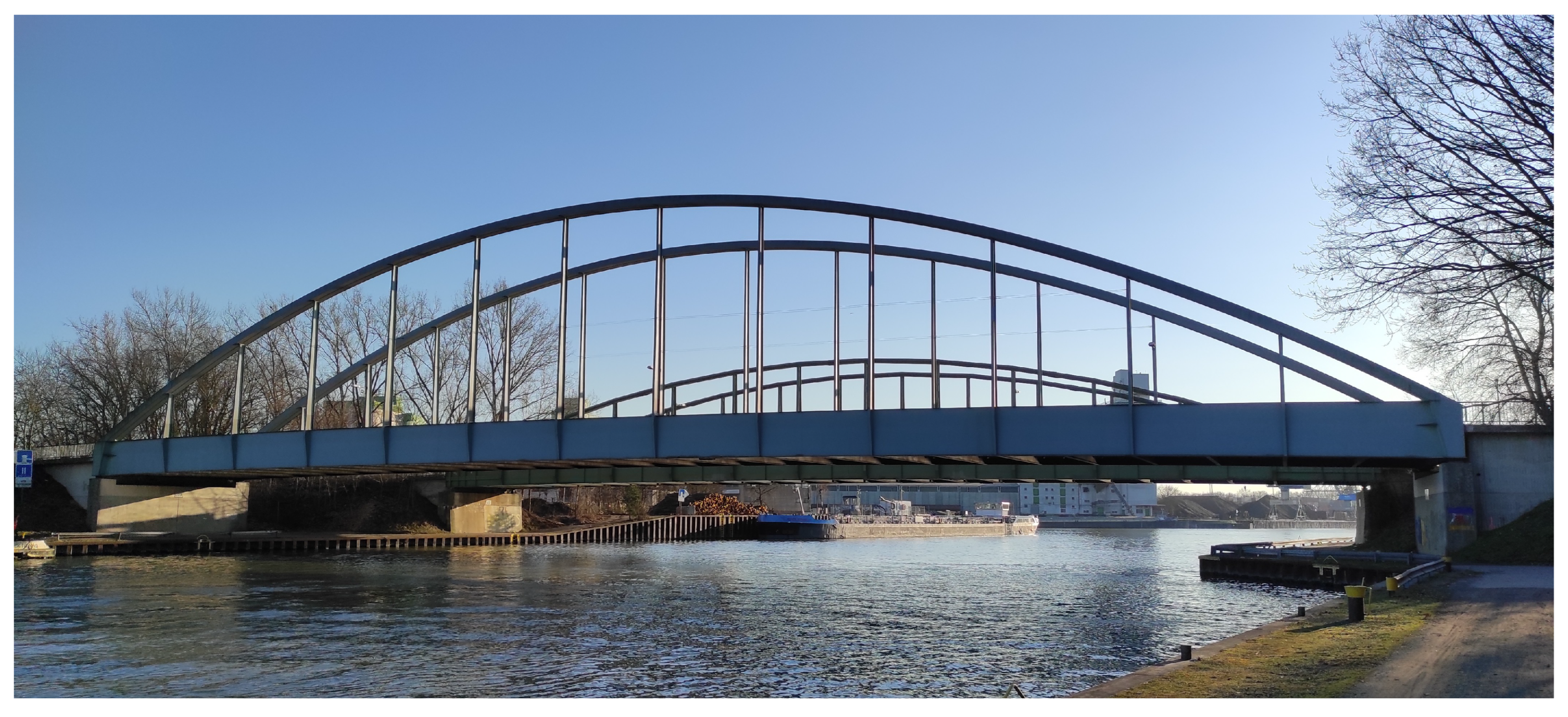
Figure 2.
Cracks in a weld connection between a hanger’s web and the top flange of the stiffening girder
Figure 2.
Cracks in a weld connection between a hanger’s web and the top flange of the stiffening girder
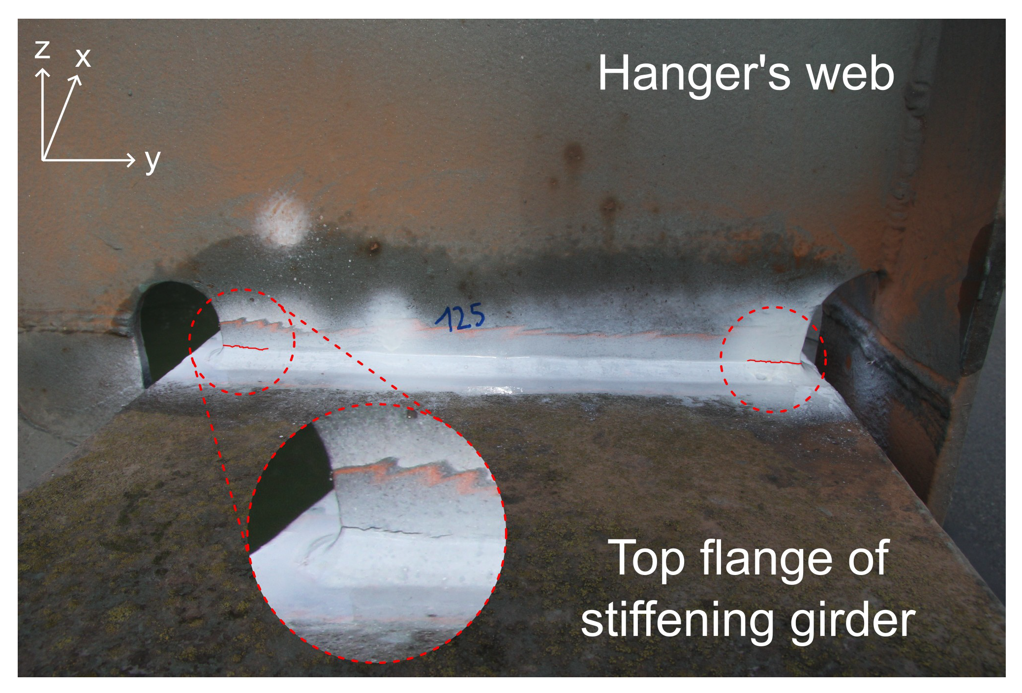
Figure 3.
Load test using a weighted truck in the middle of the bridge
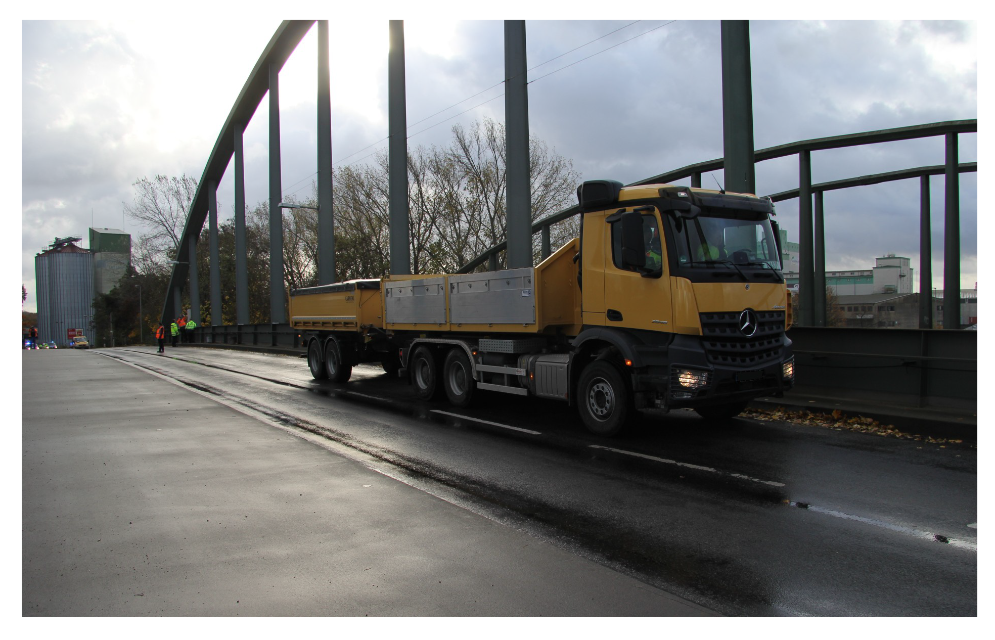
Figure 4.
Overview of the geometric model, the investigated load cases, the measurement locations, the potential damage locations, and the damage modelling
Figure 4.
Overview of the geometric model, the investigated load cases, the measurement locations, the potential damage locations, and the damage modelling
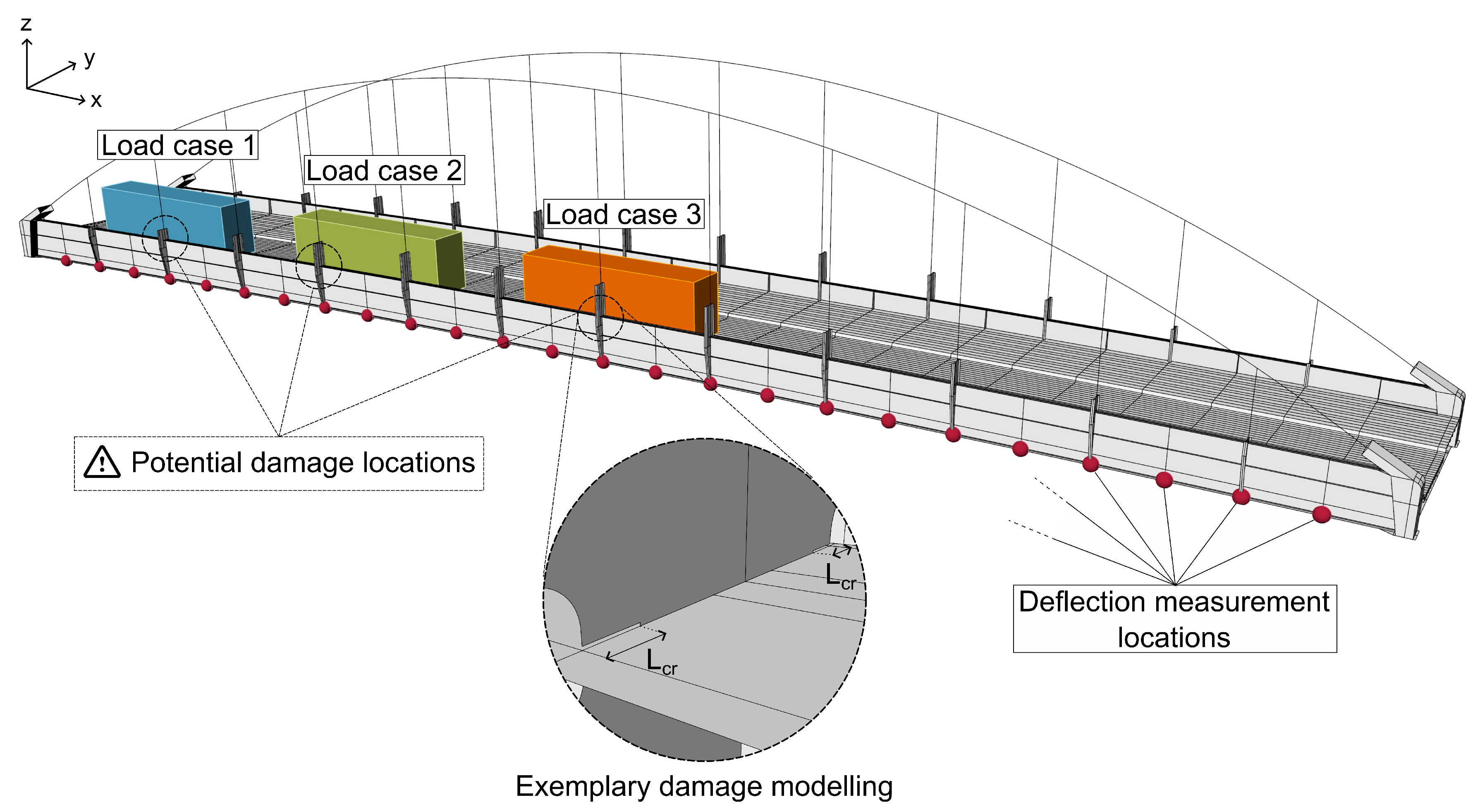
Figure 5.
Component model for the SCRBE method with the selected parameters
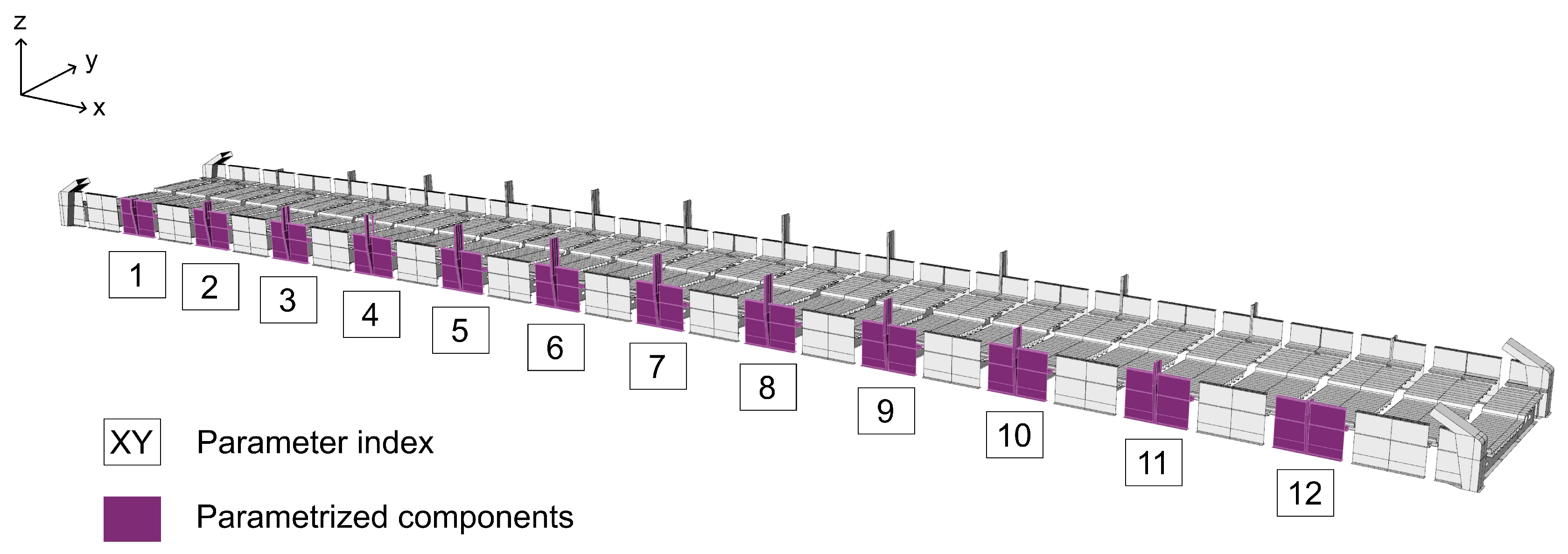
Figure 6.
Vertical displacements for three load cases at 25 deflection measurement locations
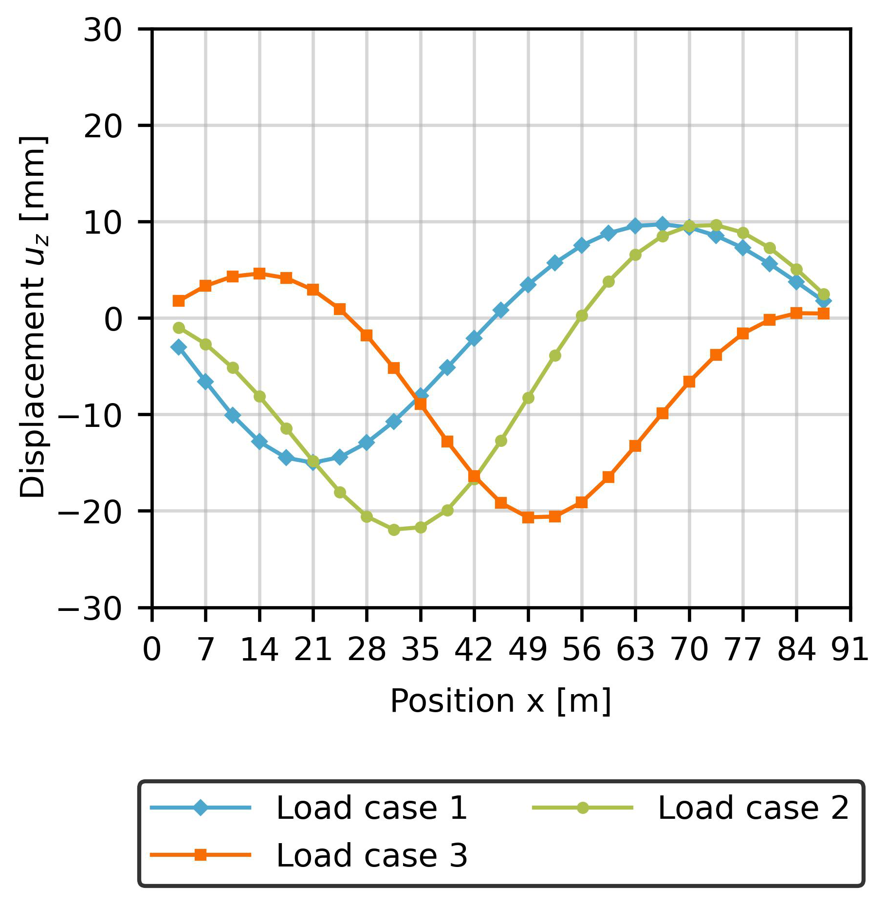
Figure 7.
Displacement alteration for damage states 1 to 4
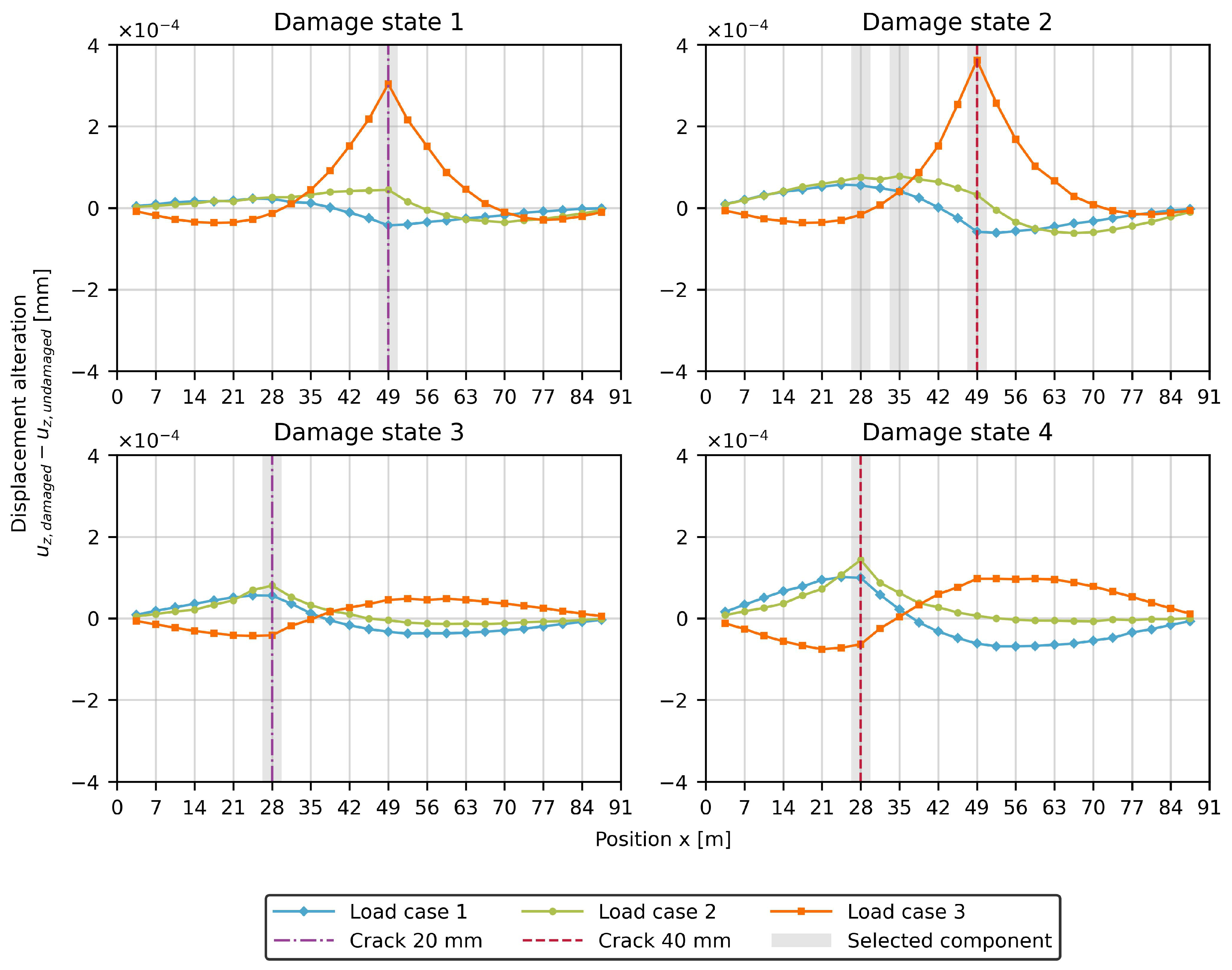
Figure 8.
Displacement alteration for damage states 5 to 8
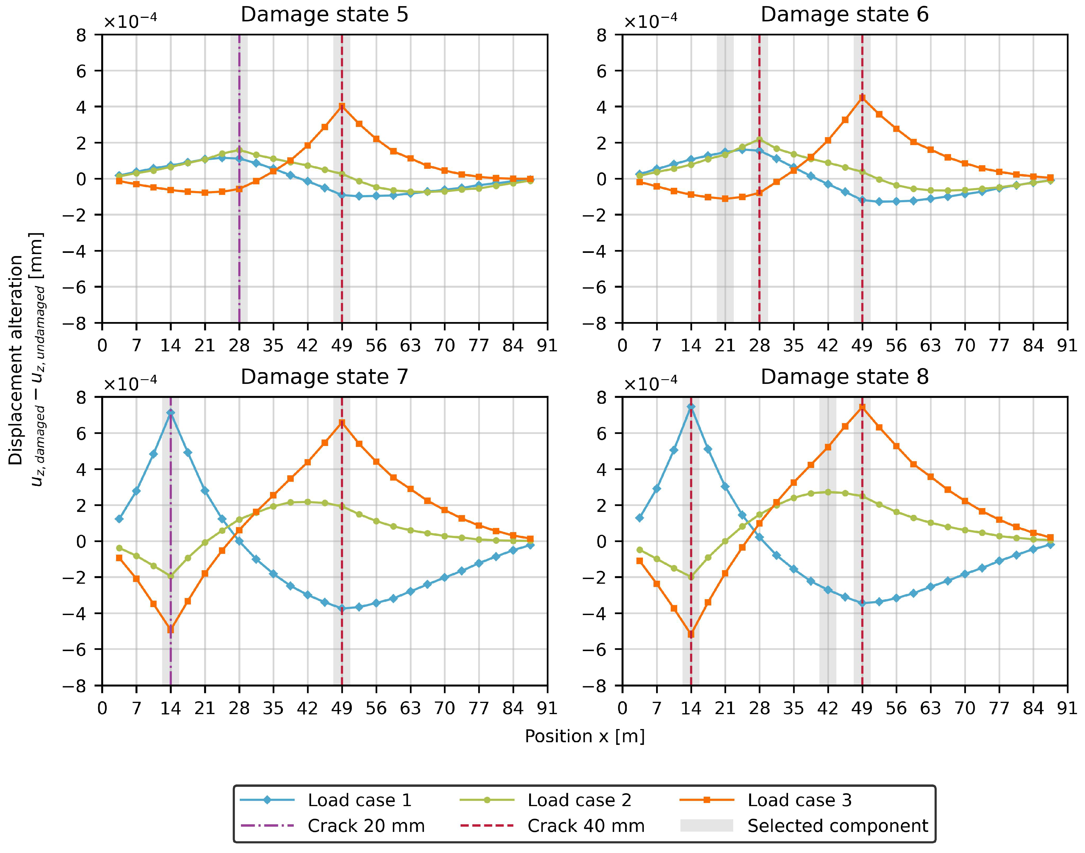
Figure 9.
Displacement alteration for damage states 9 and 10
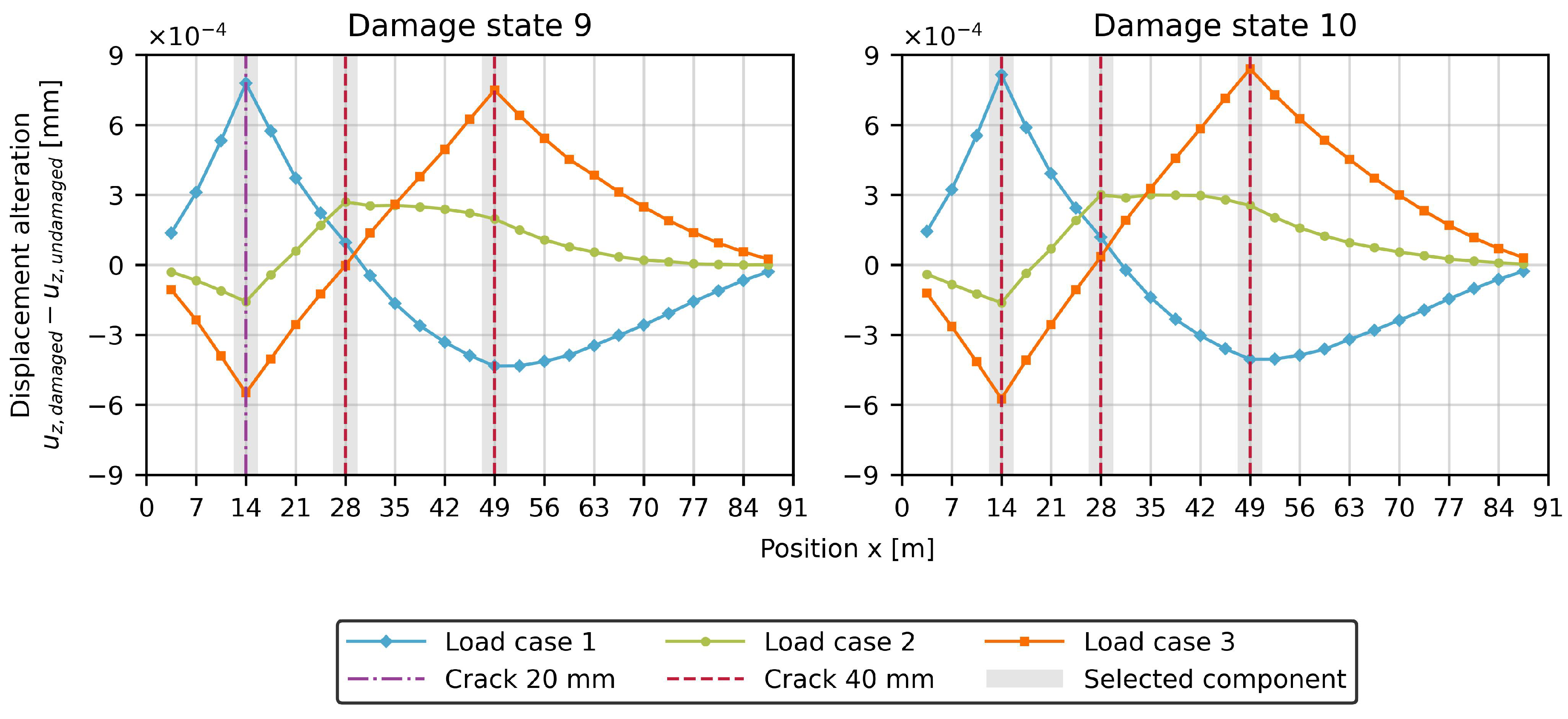
Figure 11.
Displacement alteration for damage states 5 to 8 for the calibrated model with an initial damage
Figure 11.
Displacement alteration for damage states 5 to 8 for the calibrated model with an initial damage
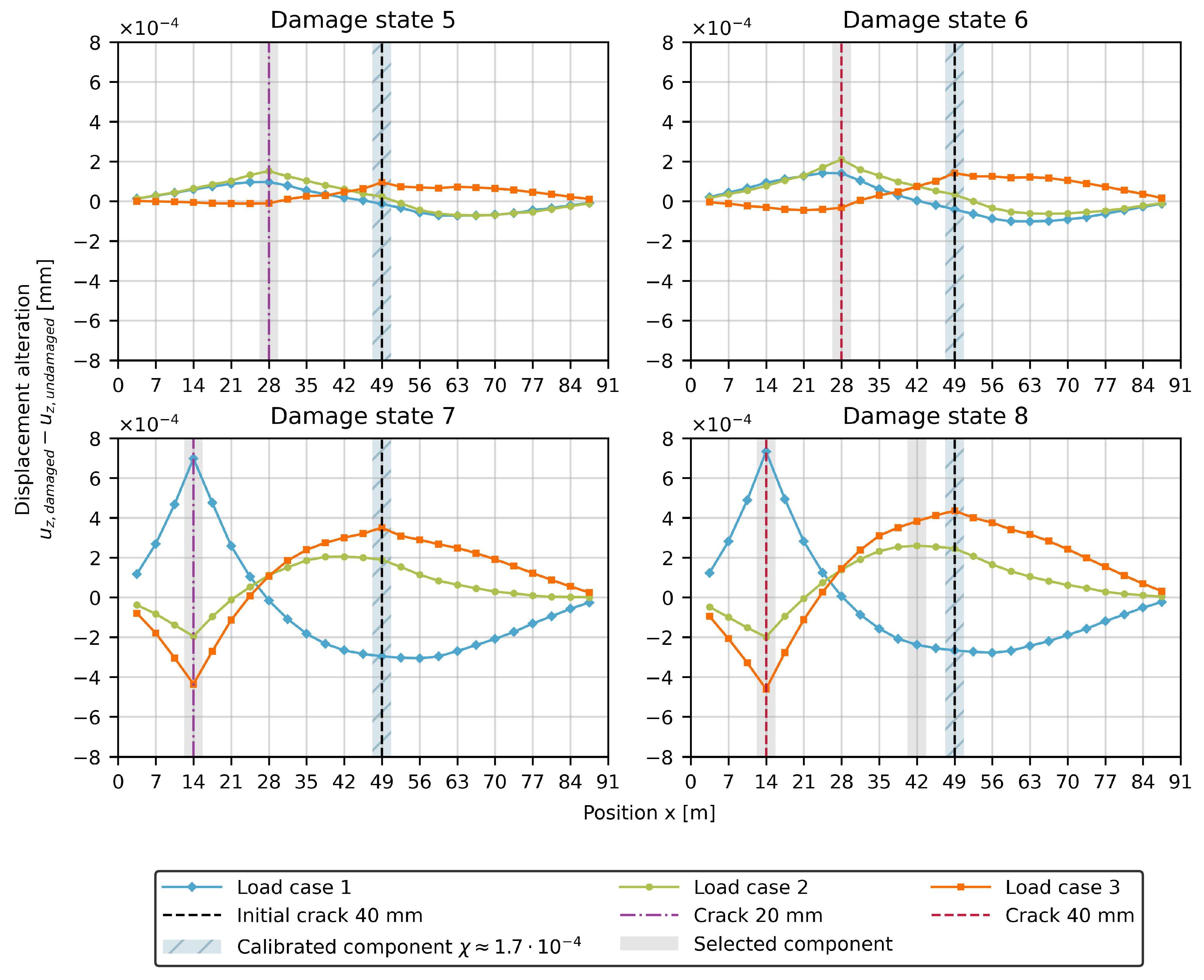
Figure 12.
Displacement alteration for damage state 9 and 10 for the calibrated model with an initial damage
Figure 12.
Displacement alteration for damage state 9 and 10 for the calibrated model with an initial damage
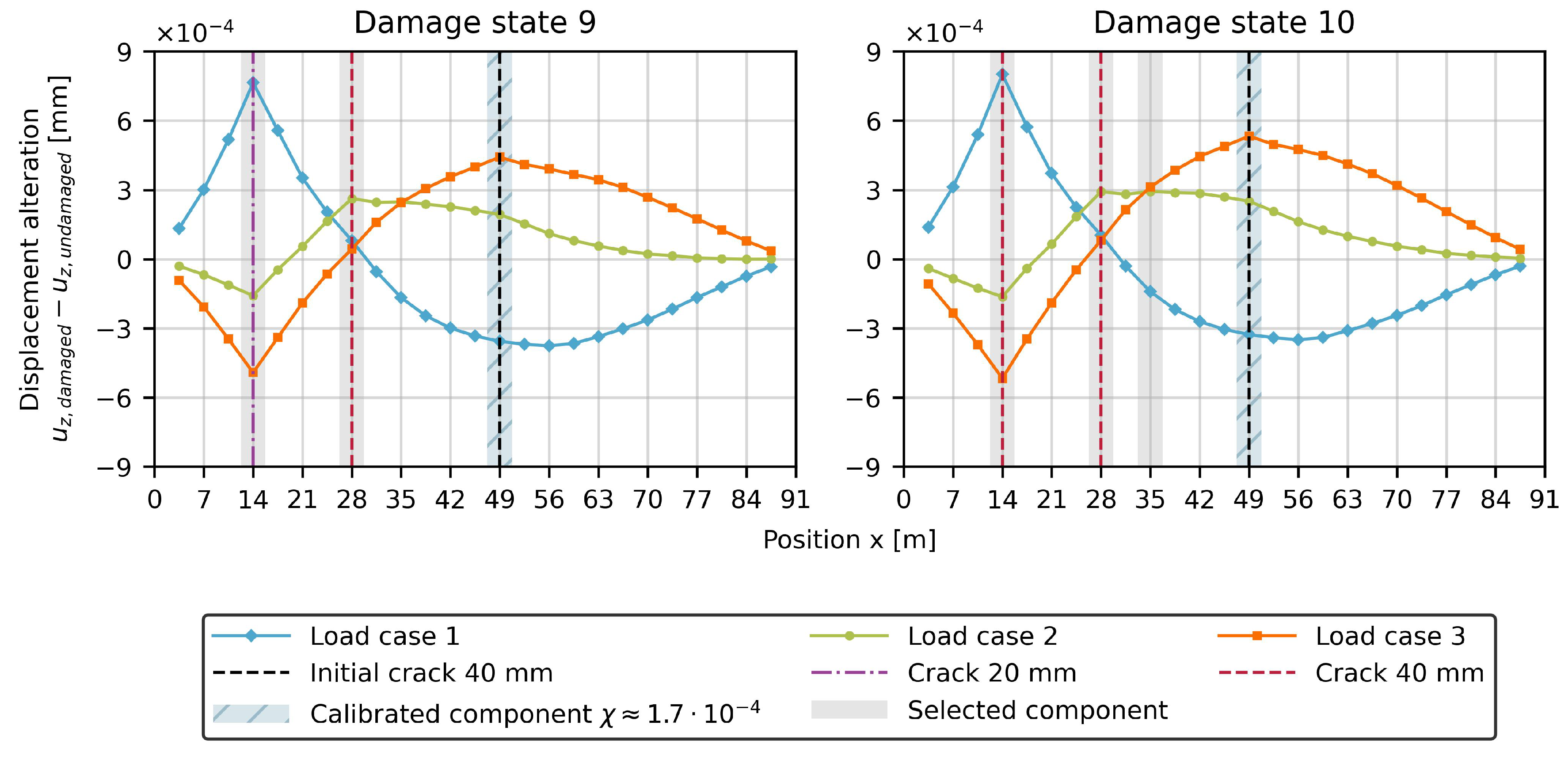

Table 1.
Investigated synthetic damage states based on the existing damages
| State Damage | Hanger 2 | Hanger 4 | Hanger 7 | ||||
|---|---|---|---|---|---|---|---|
| State Damage | |||||||
| 1 | × | ||||||
| 2 | × | ||||||
| 3 | × | ||||||
| 4 | × | ||||||
| 5 | × | × | |||||
| 6 | × | × | |||||
| 7 | × | × | |||||
| 8 | × | × | |||||
| 9 | × | × | × | ||||
| 10 | × | × | × | ||||
Disclaimer/Publisher’s Note: The statements, opinions and data contained in all publications are solely those of the individual author(s) and contributor(s) and not of MDPI and/or the editor(s). MDPI and/or the editor(s) disclaim responsibility for any injury to people or property resulting from any ideas, methods, instructions or products referred to in the content. |
© 2024 by the authors. Licensee MDPI, Basel, Switzerland. This article is an open access article distributed under the terms and conditions of the Creative Commons Attribution (CC BY) license (http://creativecommons.org/licenses/by/4.0/).
Copyright: This open access article is published under a Creative Commons CC BY 4.0 license, which permit the free download, distribution, and reuse, provided that the author and preprint are cited in any reuse.


