Submitted:
25 November 2024
Posted:
26 November 2024
You are already at the latest version
Abstract
This paper presents a cable defect assessment method based on a mixed-domain multi-feature set derived from overall harmonic signals. Four typical defect types—thermal ageing, cable moisture, excessive bending, and insulation damage—were simulated under laboratory conditions. Grounding current tests and Variational Mode Decomposition (VMD) time series analysis were performed on the test samples to extract the overall harmonic sequences in the grounding current. Mixed-domain multi-feature set is then formed through feature extraction and validity analysis. To optimize the assessment performance, a Support Vector Machine (SVM) classifier optimized by the Sparrow Search Algorithm (SSA) was constructed. The results show that different defects lead to significantly differentiated harmonic distortions in the grounding currents, which is proved to be a reliable data basis for cable defect assessment. The proposed method refines the data information and achieves the most accurate recognition of cable defects, which may contribute to the reliable operation of power networks.
Keywords:
power cable
; harmonic sequence
; mixed-domain feature extraction
; defect recognition
1. Introduction
As a core component in power transmission and communication systems, the stability and reliability of cables are crucial to the operation of the entire system. With the continuous expansion of the power network, the frequency of cable failures and the scope of influence have gradually increased. Cable failures not only lead to system shutdowns, but also may cause safety hazards. Therefore, real-time, accurate cable condition detection and defect identification technology has become an indispensable part of the power system. The development of cable condition detection technology, especially in defect identification and fault prediction, has gradually become a research hotspot.
Traditional cable inspection methods mainly include manual inspection, visual inspection and traditional electrical testing. These methods, although effective in some cases, are unable to meet the increasingly complex conditions of power systems due to manual dependence, heavy workload, and detection limitations [1]. With the development of new sensors and intelligent monitoring technologies, cable condition detection has gradually shifted to automation, real-time and high efficiency. In recent years, cable fault identification methods based on sensor data have been widely used. Sensors can provide real-time cable operation data. Through data processing and analyzing, potential problems of cables can be effectively found [2,3,16].
In addition to sensor technologies, data-driven intelligent diagnostic methods have become a focus of research. Recently, the application of machine learning and deep learning techniques in cable defect identification has made significant progress. By building models based on historical data, machine learning algorithms are able to identify potential patterns of cable faults and perform predictive maintenance [4,17]. For example, algorithms such as Support Vector Machine (SVM), Neural Network, and Random Forest (RF) in cable defect detection has shown good results [5,6]. These techniques not only improve the accuracy of cable fault detection, but also provide an early warning before a fault occurs, thus providing sufficient time for operation and maintenance personnel to carry out repairs.
Cable defects usually include problems such as insulation deterioration, mechanical damage, and high temperatures, which may lead to reduced performance or even complete failure of the cable [7,15]. Therefore, accurately identifying different types of defects and distinguishing their severity is an important task in cable condition monitoring. In recent years, the fusion application of various sensor technologies based on image processing, vibration analysis, temperature detection, etc., has made cable fault detection methods more diverse and efficient [8]. For example, infrared imaging technology has been widely used for temperature monitoring of cables in order to detect problems such as overheating and short circuits in time [9].
Despite the significant progress of existing cable defect detection techniques, some challenges still exist. For example, the issues of how to perform effective real-time monitoring in complex power system environments, how to improve the robustness and accuracy of algorithms, and how to handle data in large-scale cable networks have still not been fully addressed [10]. Therefore, future research directions should focus on improving the intelligence of cable condition detection, enhancing the fusion capability of multiple data sources, and optimising the efficiency and stability of existing detection algorithms.
Considering the current research status in cable inspection, this paper presents a cable defect assessment method based on mixed-domain multi-feature set of overall harmonic signals. Four typical defect types including thermal ageing, cable moisture, excessive bending, and insulation damage were simulated under laboratory conditions. The ground current test as well as the Variational Mode Decomposition (VMD) time series analysis are carried out on the test samples to obtain the overall harmonic sequence in the grounding current. On this basis, the mixed-domain multi-feature extraction is carried out, and the effective features are screened to form a feature set as the basis of cable defect assessment. Finally, the Sparrow Search Algorithm (SSA) is used to optimize the parameters of the original Support Vector Machine (SVM) classification model to achieve the best assessment results. Directly taking the overall harmonic sequences in the grounding current signals as the data source is equivalent to the initial refining of the signal components that contain information about cable defects at the beginning, which ensures the effectiveness of the subsequent feature extraction. This study will provide theoretical basis and technical support for the real-time condition detection of power cables, and provide guarantee for the reliable operation of power networks.
2. Harmonic Current Test
2.1. Specimen Preparation
The 10 kV XLPE cable, model YJLV 8.7/15 kV -1×70 mm², is the object of this research. Each cable specimen, 1 m in length, has been respectively subjected to four typical defects resulting from thermal ageing, cable moisture, excessive bending and insulation damage. The specific simulation methods are detailed in Table 1.
2.2. Current Collection
As illustrated in Figure 1, an experimental system is constructed. The models and parameters of each equipment in the test system are listed in Table 2. The voltage regulator and the test transformer are integrated to form a high-voltage power supply, which applies a voltage of 8.7 kV to the cable specimen. The deployment of the protective resistor serves to safeguard the test system from the potential impact of short-circuit overcurrents. The sampling resistor serves to convert the grounding current signal into a voltage signal. The data would be stored through a high-frequency acquisition card.
2.3. Harmonic Sequence Separation
The Variational Modal Decomposition (VMD) [11] is used here to perform the time series analysis of the acquired grounding current signals. This signal decomposition method can decompose the complex signal into several Intrinsic Mode Functions (IMFs) and residuals, as follows.
K represents the number of modes.
By this method, the fundamental component (with a frequency of 50 Hz) can be eliminated easily from the grounding current signal, and the overall harmonic sequence can be separated out. The overall harmonic sequences of the four cable defects are shown for example in Figure 2. These harmonic sequences will be used as the basic data for subsequent feature extraction and defect assessment.
3. Mixed-Domain Multi-Feature Set of Harmonic Sequence
3.1. Extraction Methods
Mixed-domain feature extraction is to use the different parameters presented in the time, frequency and energy domains of the signal to extract the features that can reflect the nature of the signal effectively. For the specimens of each defect type, 500 groups of the overall harmonic sequences were collected to calculate the time-domain, frequency-domain, relative energy and sample entropy feature parameters.
Time-domain features are the simplest and most direct, which are usually calculated directly on the time domain waveform of the signal, including quantitative parameters such as maximum, minimum, mean, variance, and dimensionless parameters such as peak factor and waveform factor. In general, the dimensionless indicators are only determined by the probability density function of the corresponding signals, while the quantitative indicators will be affected by the environment and the acquisition working conditions.
Frequency-domain features are obtained on the basis of the signal power spectrum. The signal power spectrum means the signal power per unit frequency band, which represents the signal power variation with frequency, that is, the distribution of signal power in the frequency domain [12]. The average power of over can be represented as (2).
Express as during the period , Thus the Fourier transform is . Suppose that when , tends to a limit. The average power can be transformed into
Define as the power density function of . Then the power spectrum is
The power spectrum mean, centre-of-gravity frequency, frequency variance, frequency standard deviation, mean square frequency and root-mean-square frequency are obtained by calculating the power spectrum of the harmonic sequences. The mean value of the power spectrum reflects the energy size of the power spectrum, the standard deviation of the frequency describes the degree of dispersion or concentration of the frequency spectrum, and the centre-of-gravity frequency and the root-mean-square frequency reflect the change in position of the main frequency band. The formulae of time-domain and frequency-domain features are shown in Table 3.
In addition, multi-scale relative energy and sample entropy features are extracted. Due to the different types of evolving physical processes and different degrees of complexity, the energy distribution and entropy value of different defective cables are bound to have large differences. In this paper, the wavelet packet decomposition algorithm is used to calculate the energy features. The principle of wavelet packet decomposition is shown in Figure 3, where X0 represents the original signal, L represents the low-frequency part, and H represents the high-frequency part. Unlike wavelet decom position which decomposes only the low frequency part of the signal, wavelet packet decomposition does decomposition processing for the high frequency part as well. When the j-layer wavelet packet decomposition is carried out, the energy values can further be calculated and normalized into relative energy values for each subband, according to (5).
Meanwhile, the entropy value of each subband signal sample can also be calculated. The subband sample entropy sequence is represented as SampEn(k), . The db1 wavelet is chosen here to decompose the harmonic sequence in 3 layers of wavelet packets.
In summary, this study extracted 16 time-domain feature parameters, 6 frequency-domain feature parameters, and 16 multi-scale relative energy and sample entropy parameters, a total of 38 feature parameters, which are used the preparatory assessment basis of power cable defect recognition.
3.2. Feature Validity Analysis
For the quantitative time-domain features, histograms are used to describe them. Figure 4 demonstrates the distribution range of the maximum and peak-to-peak values of the overall harmonic sequences. It can be found that the harmonic peak distribution range is related to the defect type, and the harmonic changes caused by thermal ageing are the most obvious, with the maximum value of the total harmonic sequence reaching up to 588.76 μA, and the peak-to-peak value reaching up to 972.50 μA. Harmonic changes caused by excessive bending are the next most obvious, with the maximum value in the range of 175.40 ~ 248.92 μA, and the distribution of the peak-to-peak value in the range of 356.72 ~ 566.21 μA.
For other dimensionless features, if the distribution of the feature parameter is more concentrated under the same cable defect, it means that the parameter describes the cable defect condition more consistently. If there is less overlap in the distribution of the characteristic parameter under different cable defects, it means that the parameter has a higher degree of differentiation between cable defects. In statistics, box plots are often used to describe the degree of concentration and dispersion of data. The distribution of dimensionless time-domain feature parameters is shown in Figure 5, the distribution of some frequency-domain feature parameters is shown in Figure 6 and the distribution of multi-scale relative energy and sample entropy parameters is shown in Figure 7.
As for the dimensionless time-domain features, it can be found from Figure 5 that under different cable defects, the distribution ranges of waveform factor and cliff factor have almost no overlap, which can effectively distinguish cable defects. The distribution ranges of impulse factor, margin factor and skew factor have more overlapping parts, which can't effectively distinguish cable defects. The peaking factor can distinguish two kinds of defects, cable moisture and excessive bending.
Regarding the frequency-domain parameters, it can be found in Figure 6 that the power spectrum mean has a high degree of differentiation between the four defects. The distribution range of frequency standard deviation overlaps more and cannot distinguish the cable defects. In addition, the centre-of-gravity frequency and the root-mean-square frequency can only distinguish the excessive bending damage from the other three cable defects.
For the multi-scale relative energy and sample entropy features, the result show that the overall harmonic sequence energy of the defective cable is mainly concentrated in the low-frequency subbands LLL3, HLL3 and LHL3, especially LLL3. Therefore, the relative energy and sample entropy features of the other five subbands are omitted in consideration of the feature validity. As can be seen in Figure 7, the relative energy features of subbands LLL3, HLL3, and LHL3 can distinguish excessive bending damage, but for the other three defects there is a partial overlap in the distribution range. The sample entropy feature parameters of subbands LLL3, HLL3 and LHL3 have more overlapping distribution ranges and cannot be used as effective features to distinguish cable defects.
By extracting and analyzing the time-domain, frequency-domain, multi-scale relative energy and sample entropy feature parameters of the overall harmonic signal of the grounding current, the feature parameters that obviously cannot distinguish the cable defects are excluded, and finally 14 feature parameters are retained as the effective feature parameters for the assessment of cable defects. The mixed-domain multi-feature sets of the harmonic series include maximum, peak-to-peak, absolute mean, standard deviation, root-mean-square, waveform factor, peak factor, cliff factor, power spectrum mean, centre-of-gravity frequency, root-mean-square frequency, LLL3 relative energy, HLL3 relative energy and LHL3 relative energy.
4. Improved SVM Model for Cable Defect Recognition
4.1. Support Vector Machine (SVM)
If the mixed-domain multi-feature set, which contains 14 feature parameters, is directly used as the input of the classifier, it is very computationally intensive and prone to dimensionality catastrophe. Therefore, to alleviate the model computational burden, Principal Component Analysis (PCA) is firstly used to fuse feature set down to 3 dimensions before the model is built, which will not be repeated here [13].
Support Vector Machine (SVM) was proposed by Cortes and Vapnik in 1995. Compared with neural network classifiers, SVMs show unique advantages in dealing with small samples, high-dimensional patterns and nonlinear problems. It is essentially a convex programming problem with a globally optimal solution, which can avoid the problem of model convergence to local extremes. When the input samples are nonlinear, the kernel function needs to be introduced. Using the kernel function, the data can be mapped into a high-dimensional space, thus solving the problem that the data samples are linearly indivisible in the original space. In this paper, we choose the RBF kernel function. This kernel function is widely used and simple to compute, but the choice of parameter σ has a great impact on the prediction accuracy of the model. inappropriate choices may lead to issues such as overfitting or underlearning.
RBF kernel function expression is:
where σ is the variance of the radial basis function.
Therefore, using an effective method to find the optimal penalty factor C and kernel parameter σ is the key to exploit the optimal performance of SVM.
4.2. Model Improvement Through Sparrow Search Algorithm (SSA)
For the problem of difficult SVM parameter setting, Sparrow Search Algorithm (SSA) is adopted to find the optimal of the important parameters, the penalty factor C and the kernel parameter σ. The idea of SSA originates from the analysis of sparrow's foraging and hazard avoidance behaviours, and the advantage lies in the rapid convergence, accurate identification and strong robustness [14].
SSA classifies foraging sparrow groups into three types: discoverers, followers and vigilantes. Discoverers are part of the individuals in the sparrow population that are responsible for leading the search for food, and followers are part of the individuals that follow the discoverers in their foraging activities. During the whole foraging activity, some individuals from the discoverers and followers are responsible for detecting and guarding, and when there is danger, they give up foraging and engage in avoidance behaviours. The corresponding location information of each individual sparrow is updated iteratively as the foraging process proceeds.
The flow of the optimization is shown in Figure 8, and the specific steps are as follows:
- (1)
- Initialize the SSA parameters, which include the number of sparrow groups, the maximum number of iterations, the ratios of discoverers and followers and vigilantes, and also the range of C and σ values;
- (2)
- Calculate and rank the fitness of each sparrow, and classify the group to which they belong;
- (3)
- Update the positions of the sparrows in the three groups according to the position update rule;
- (4)
- After the position update, calculate the fitness value of each sparrow again, compare the fitness values before and after the update, keep the optimal fitness, and continue the update;
- (5)
- Determine whether the termination condition of the algorithm is satisfied or whether the maximum number of iterations is reached, if so, output the optimal parameters C, σ, otherwise, return to step (2) to continue the iteration until the termination condition is satisfied.
The parameter settings of SSA are shown in Table 4. The value range of parameter C is set to (0.01, 100) and the value range of parameter σ is set to (0.1, 100).
4.3. Testing Result and Comparison
The fitness change curve of the SSA-SVM model is shown in Figure 9. It can be seen that the iteration to the 6th generation has reached the optimal fitness, the optimal fitness value is 0.0225, at this time the corresponding penalty factor C takes the value of 0.6121, and the kernel parameter σ takes the value of 16.4067.
Each cable defect corresponds to 500 groups of principal component matrices Y, and the four cable defects form an input matrix of dimension 2000 × 3, of which 1600 groups of samples are selected randomly for SVM training, and the remaining 400 groups are used for testing. The recognition results of the SSA-SVM are shown in Figure 10. The result shows that the SSA-SVM model can successfully distinguish the four types of cable defects, and for each defect in the test set, the recognition rate can reach 100 %. The classification effect is significant.
In addition, the SVM model without parameter optimization as well as the BPNN model are used as comparisons. As can be seen from Table 5, the SVM model optimized by SSA is quite more accurate than the SVM model and the BPNN model, reaching 100% after feature fusion. In the SVM model, the penalty factor C is usually directly set to 100 and the kernel parameter σ is set to 0.1, whereas SSA can obtain the best parameter values for the current problem through the optimization search process. The classification recognition accuracy is therefore improved. In addition, after PCA feature fusion, the recognition rates of SVM model, BPNN model and SSA-SVM model are improved, which also makes the algorithm take obviously less time. However, compared with the SVM model and BPNN model, the overall time consumption of SSA-SVM model is much longer, and how to improve the efficiency of the algorithm while guaranteeing a high recognition rate needs to be further investigated.
5. Conclusions
In this study, four typical cable defects, namely thermal aging, cable moisture, excessive bending and insulation damage, are simulated in the laboratory, grounding current testing and VMD time series analysis are carried out to obtain the overall harmonic sequence of grounding current. Mixed-domain multi-feature set is then formed through feature extraction and validity analysis. An SSA-SVM defect recognition model is finally established to assess the cable condition. The main conclusions are as follows:
- (1)
- The results of grounding current test and VMD time series analysis show that different kinds of cable defects lead to significantly differentiated harmonic distortions in the grounding current waveforms, which can be used as a reliable basis for assessing defects in cables.
- (2)
- The time-domain, frequency-domain, multi-scale relative energy and sample entropy characteristic parameters of the overall harmonic sequences are extracted in this study. Through feature validity analysis, it is found that the maximum, peak-to-peak, absolute mean, standard deviation, root-mean-square, waveform factor, peak factor, cliff factor, power spectrum mean, centre-of-gravity frequency, root-mean-square frequency, LLL3 relative energy, HLL3 relative energy and LHL3 relative energy, in total, 14 characteristic parameters have a good differentiation of cable defects, a total of 14 feature parameters have a good differentiation of cable defects.
- (3)
- For the cable defect recognition problem, the optimal values of C and σ in the SVM model are found to be 0.6121 and 16.4067 respectively by SSA algorithm. The results show that the SSA-SVM model is effective in the cable defect recognition, which is significantly better than the SVM model as well as the BPNN model, and the recognition rate reaches 100%.
- (4)
- Although the SSA-SVM model greatly improves the accuracy of cable defect assessment, the algorithm is very time-consuming. How to improve the computational efficiency of the model while ensuring a high recognition rate is the focus of subsequent research.
Author Contributions
Conceptualization, R.D.; methodology, R.Z.; software, R.D.; validation, R.D. and R.Z.; formal analysis, R.D.; investigation, R.D.; resources, R.Z.; data curation, R.Z.; writing—original draft preparation, R.D.; writing—review and editing, R.Z. All authors have read and agreed to the published version of the manuscript.
Funding
This research received no external funding.
Data Availability Statement
The data presented in this study are available on request from the corresponding author. The data are not publicly available due to privacy reasons.
Conflicts of Interest
The authors declare no conflict of interest.
References
- Lu, H.; Zhang, W.H.; Wang, Y.; Xiao, X. Y. Cable Incipient Fault Identification Method Using Power Disturbance Waveform Feature Learning. IEEE Access. 2022, 10, 86078–86091. [Google Scholar] [CrossRef]
- De Clippelaar, S.; Kruizinga, B.; van der Wielen, P. C. J. M.; Wouters, P. A. A. F. Wave-Velocity Based Real-Time Thermal Monitoring of Medium-Voltage Underground Power Cables. IEEE Trans. Power Delivery. 2024, 39, 983–991. [Google Scholar] [CrossRef]
- Liu, Y.; Xin, Y.; Huang, Y.; Du, B.; Huang, X.; Su, J. Optimal Design and Development of Magnetic Field Detection Sensor for AC Power Cable. Sensors. 2024, 24, 2528. [Google Scholar] [CrossRef] [PubMed]
- Hu, S.; Wang, L.; Mao, J.; Gao, C.; Zhang, B.; Yang, S. Synchronous Online Diagnosis of Multiple Cable Intermittent Faults Based on Chaotic Spread Spectrum Sequence. IEEE Trans. Dielectr. Electr. Insul. 2019, 66, 3217–3226. [Google Scholar] [CrossRef]
- Abu-Rub, O. H.; Khan, Q.; Refaat S., S.; Nounou, H. Cable Insulation Fault Identification Using Partial Discharge Patterns Analysis. IEEE Canadian Journal of Electrical and Computer Engineering 2020, 45, 31–41. [Google Scholar] [CrossRef]
- Zhang, H. Cable Fault Detection and Diagnosis Method Based on Convolutional Neural Network. 2023 IEEE International Conference on Image Processing and Computer Applications (ICIPCA), Changchun, China, 2023, pp. 1463–1466.
- Liu, J.; Wang, S.; Yan, S.; Zhang, M.; Huang, L. Fast Detection Method on Water Tree Aging of MV Cable Based on Nonsinusoidal Response Measurement. IEEE Trans. Power Delivery. 2023, 38, 146–153. [Google Scholar] [CrossRef]
- Yuan, L.; Liu, W.; Zhao, Y. Multi-point sensing system for cable fault detection using fiber Bragg grating. Optical Fiber Chnology. 2024, 87, 103942. [Google Scholar] [CrossRef]
- Liu, K.; Yang, Z.; Wei, W.; Gao, B.; Xin, D.; Sun, C.; Gao, G.; Wu, G. Novel detection approach for thermal defects: Study on its feasibility and application to vehicle cables. High Voltage 2023, 8, 358–367. [Google Scholar] [CrossRef]
- Xie, J.; Sun, T.; Zhang, J.; Ye, L.; Fan, M.; Zhu, M. Research on Cable Defect Recognition Technology Based on Image Contour Detection. 2021 2nd International Conference on Big Data & Artificial Intelligence & Software Engineering (ICBASE), Zhuhai, China, 2021, pp. 387–391.
- Dragomiretskiy, K.; Zosso, D. Variational mode decomposition. IEEE Trans. Signal Processing. 2013, 62, 531–544. [Google Scholar] [CrossRef]
- Liu, Y.; Wang, H.; Zhang, H. Du, B. Thermal Aging Evaluation of XLPE Power Cable by Using Multidimensional Characteristic Analysis of Leakage Current. Polymers. 2022, 14, 3147. [Google Scholar] [CrossRef] [PubMed]
- He, K.; Li, X. Time–Frequency Feature Extraction of Acoustic Emission Signals in Aluminum Alloy MIG Welding Process Based on SST and PCA. IEEE Access. 2019, 7, 113988–113998. [Google Scholar] [CrossRef]
- Xue, J. Research and Application of A Novel Swarm Intelligence Optimization Technique: Sparrow Search Algorithm.. Master’s Thesis, Donghua University, Shanghai, China, 2020. [Google Scholar]
- Lu, X.; Hu, R.; Guo, K.; Lan, R.; Tian, J.; Wei, Y.; Li, Guo. Effect of Interface Defects on the Electric–Thermal–Stress Coupling Field Distribution of Cable Accessory Insulation. Energies. 2024, 17, 4498. [Google Scholar] [CrossRef]
- Su, J.; Zhang, P.; Huang, X.; Pang, X.; Diao, Xun.; Li, Y. Current Measurement of Three-Core Cables via Magnetic Sensors. Energies. 2024, 17, 4007. [Google Scholar] [CrossRef]
- Chen, W.; Yang, Z.; Song, J.; Zhou, L.; Xiang, L.; Wang, X.; Hao, C.; Fan, X. A High-Resolution Defect Location Method for Medium-Voltage Cables Based on Gaussian Narrow-Band Envelope Signals and the S-Transform. Energies. 2024, 17, 2218. [Google Scholar] [CrossRef]
Figure 1.
The experimental system.
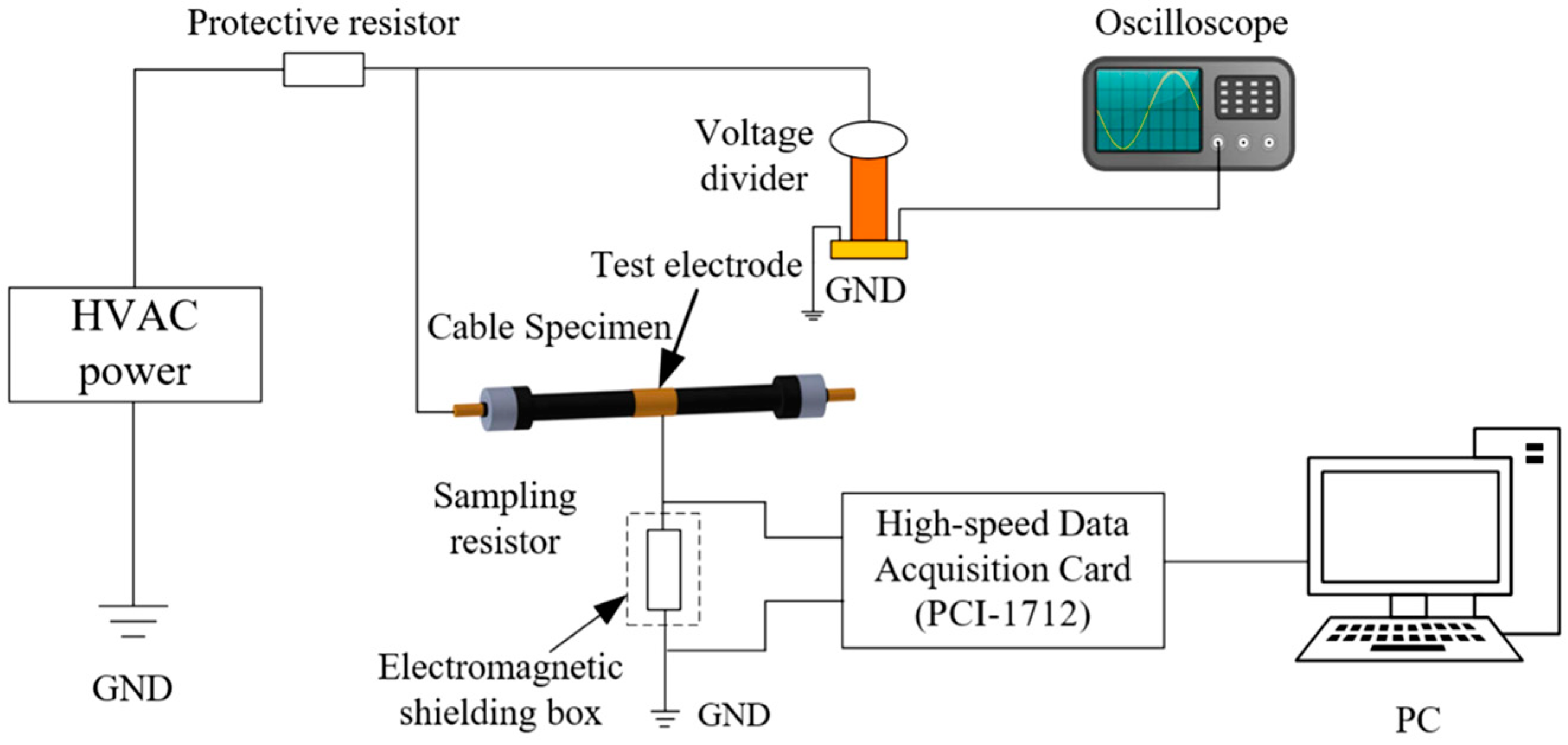
Figure 2.
The overall harmonic sequences of specimens with the four defects. (a) Thermal ageing; (b)Cable moisture; (c) Excessive bending; (d) Insulation damage.
Figure 2.
The overall harmonic sequences of specimens with the four defects. (a) Thermal ageing; (b)Cable moisture; (c) Excessive bending; (d) Insulation damage.
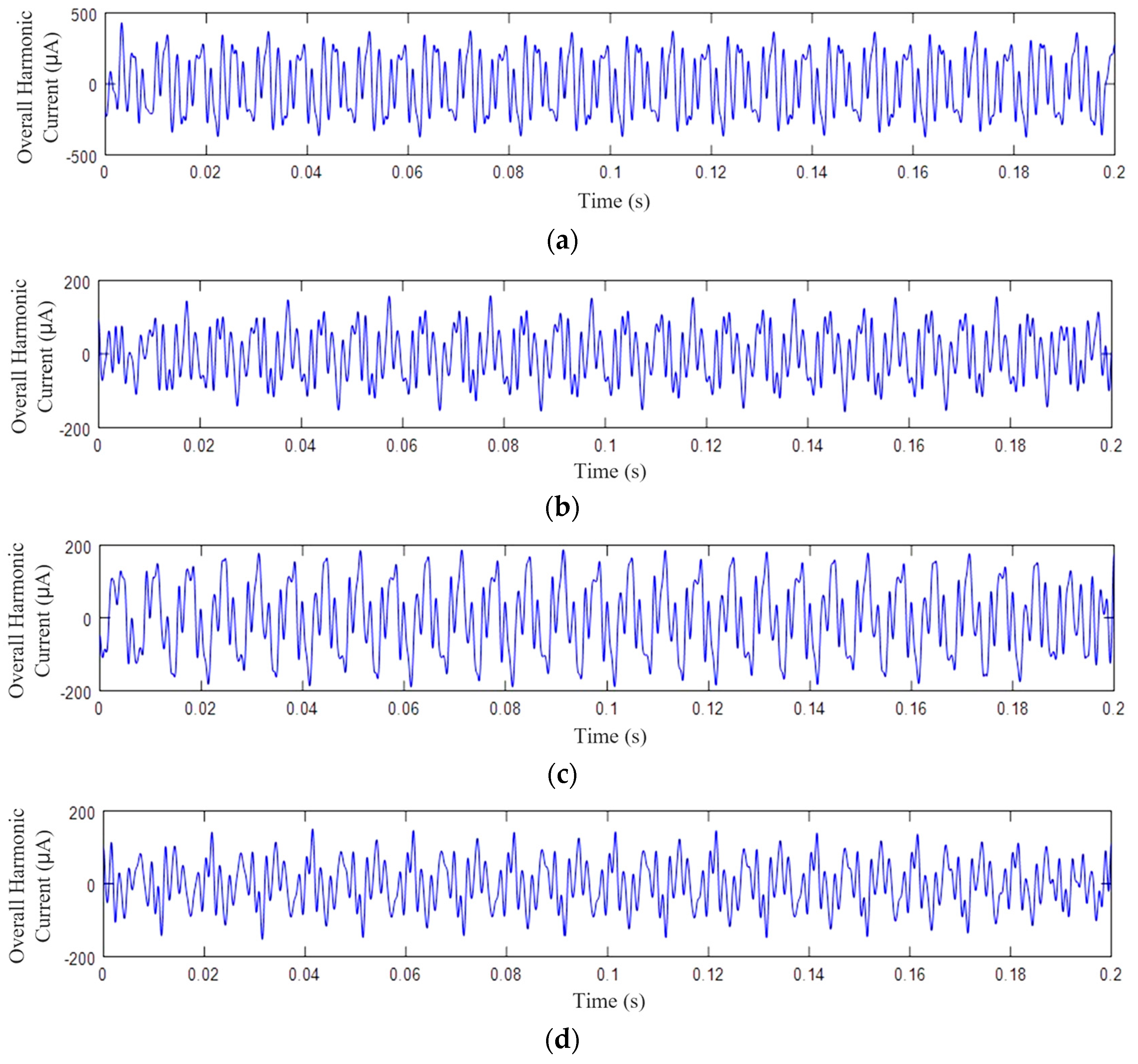
Figure 3.
Principle of wavelet packet decomposition.
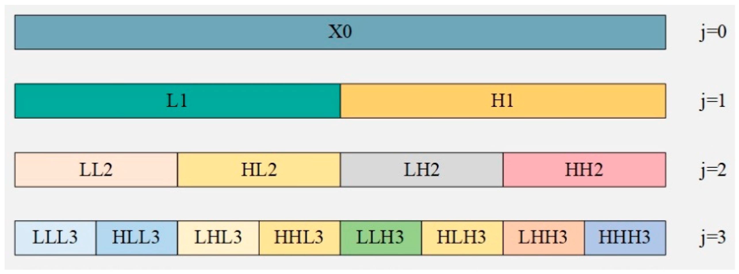
Figure 4.
The distribution range of two quantitative time-domain features: (a) Maximum; (b) Peak-to-peak.
Figure 4.
The distribution range of two quantitative time-domain features: (a) Maximum; (b) Peak-to-peak.
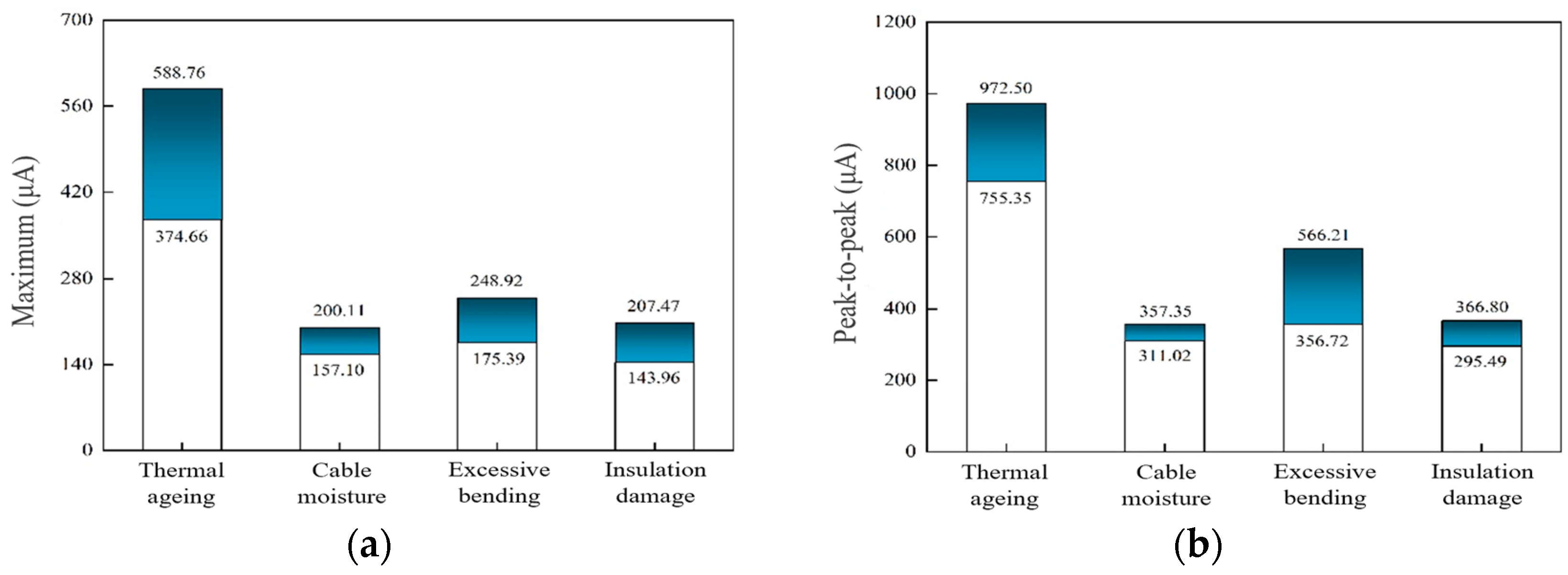
Figure 5.
The distribution range of dimensionless time-domain features: (a) Peak Factor; (b) Waveform Factor; (c) Impulse Factor; (d) Margin factor; (e) Skew factor; (f) Cliff factor.
Figure 5.
The distribution range of dimensionless time-domain features: (a) Peak Factor; (b) Waveform Factor; (c) Impulse Factor; (d) Margin factor; (e) Skew factor; (f) Cliff factor.
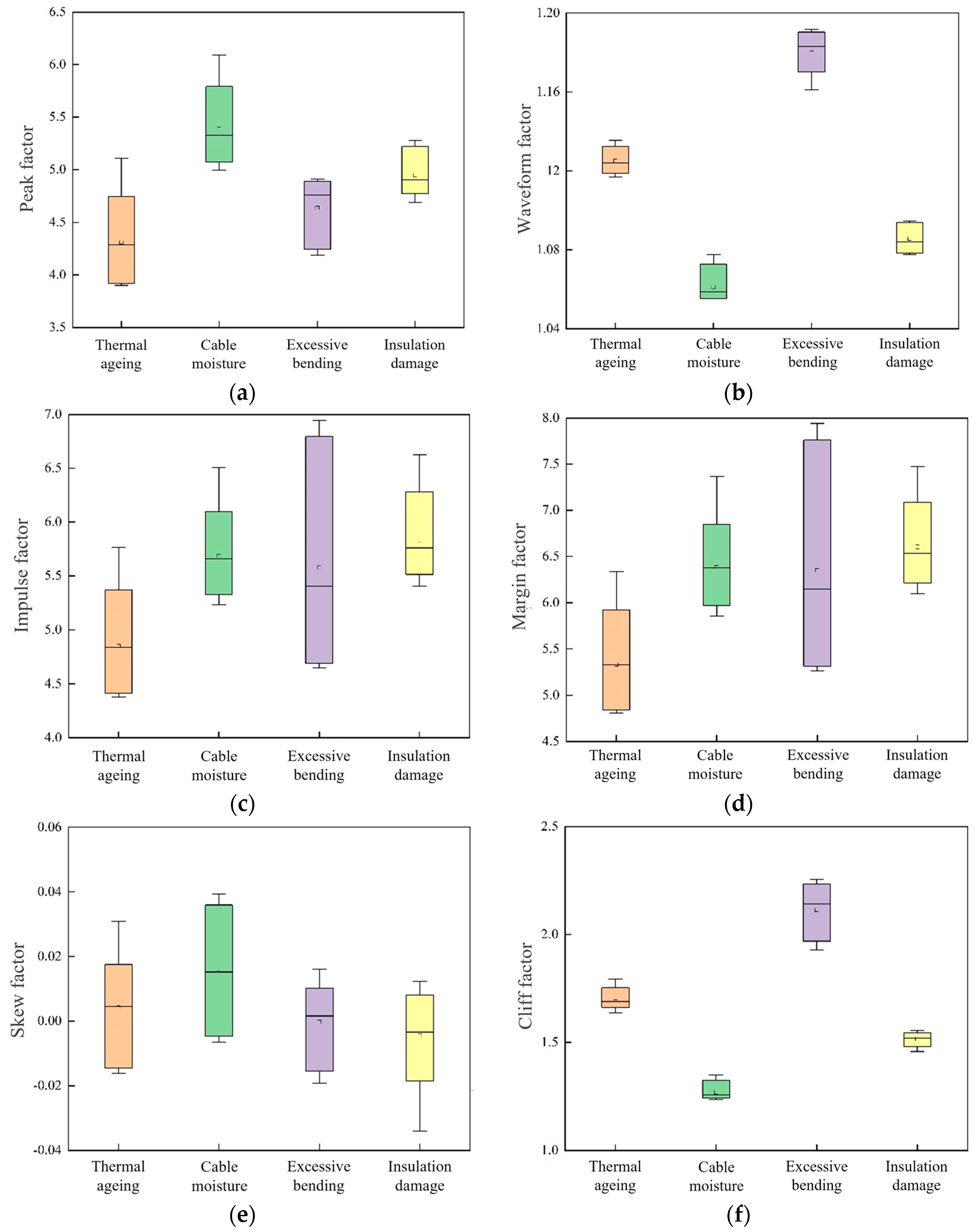
Figure 6.
The distribution range of some frequency-domain features: (a) Power spectrum mean; (b) Centre-of-gravity frequency; (c) Frequency standard deviation; (d) Root-mean-square frequency.
Figure 6.
The distribution range of some frequency-domain features: (a) Power spectrum mean; (b) Centre-of-gravity frequency; (c) Frequency standard deviation; (d) Root-mean-square frequency.
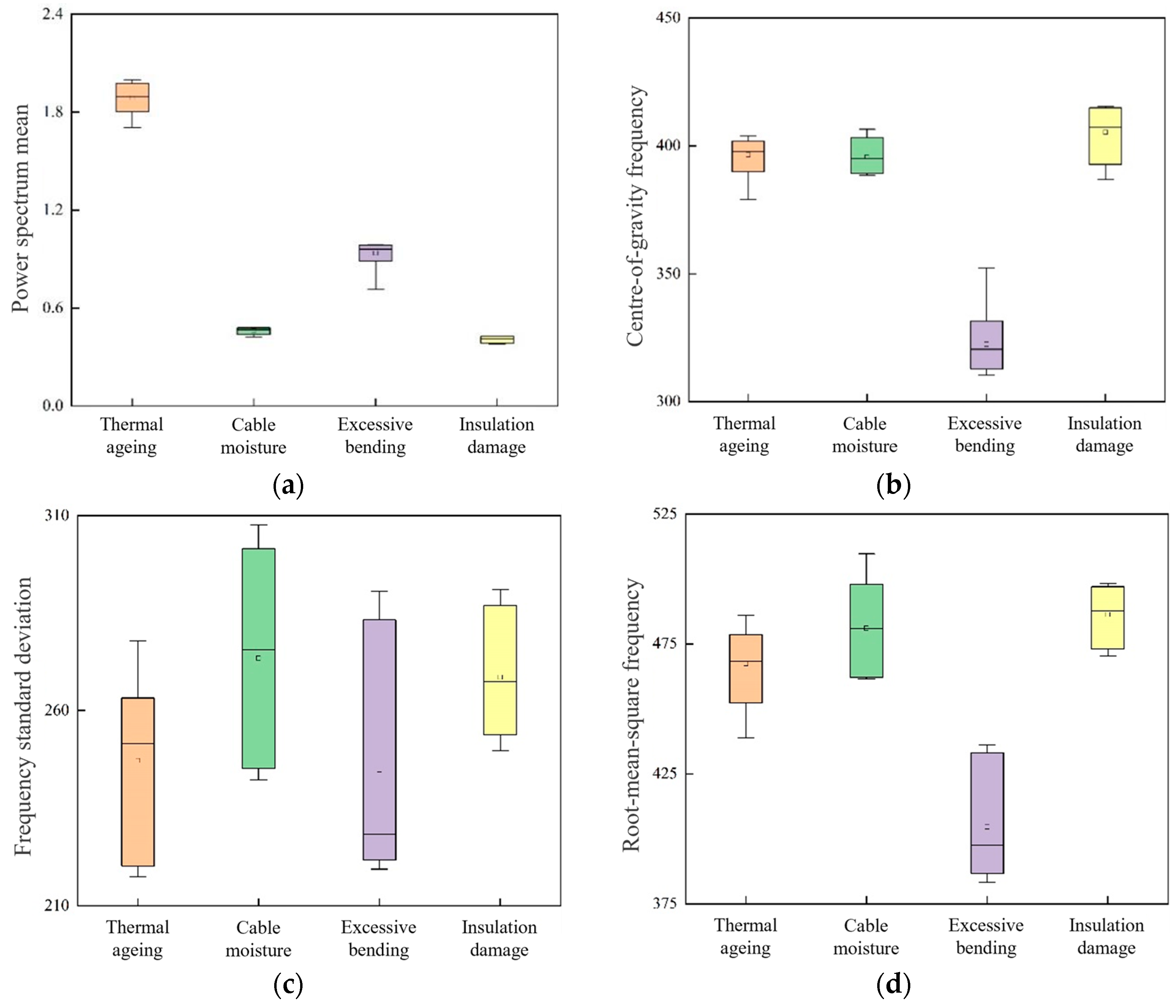
Figure 7.
The distribution range of multi-scale relative energy and sample entropy features: (a) LLL3 relative energy; (b) LLL3 sample entropy; (c) HLL3 relative energy; (d) HLL3 sample entropy; (e) LHL3 relative energy; (f) LHL3 sample entropy.
Figure 7.
The distribution range of multi-scale relative energy and sample entropy features: (a) LLL3 relative energy; (b) LLL3 sample entropy; (c) HLL3 relative energy; (d) HLL3 sample entropy; (e) LHL3 relative energy; (f) LHL3 sample entropy.
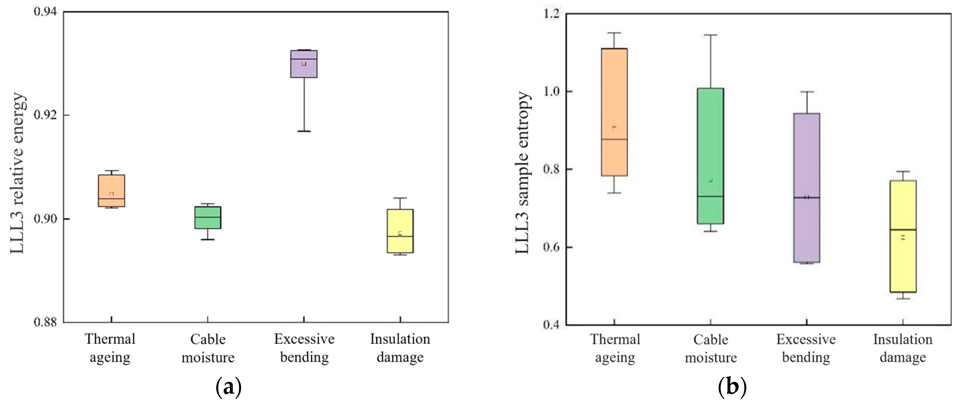
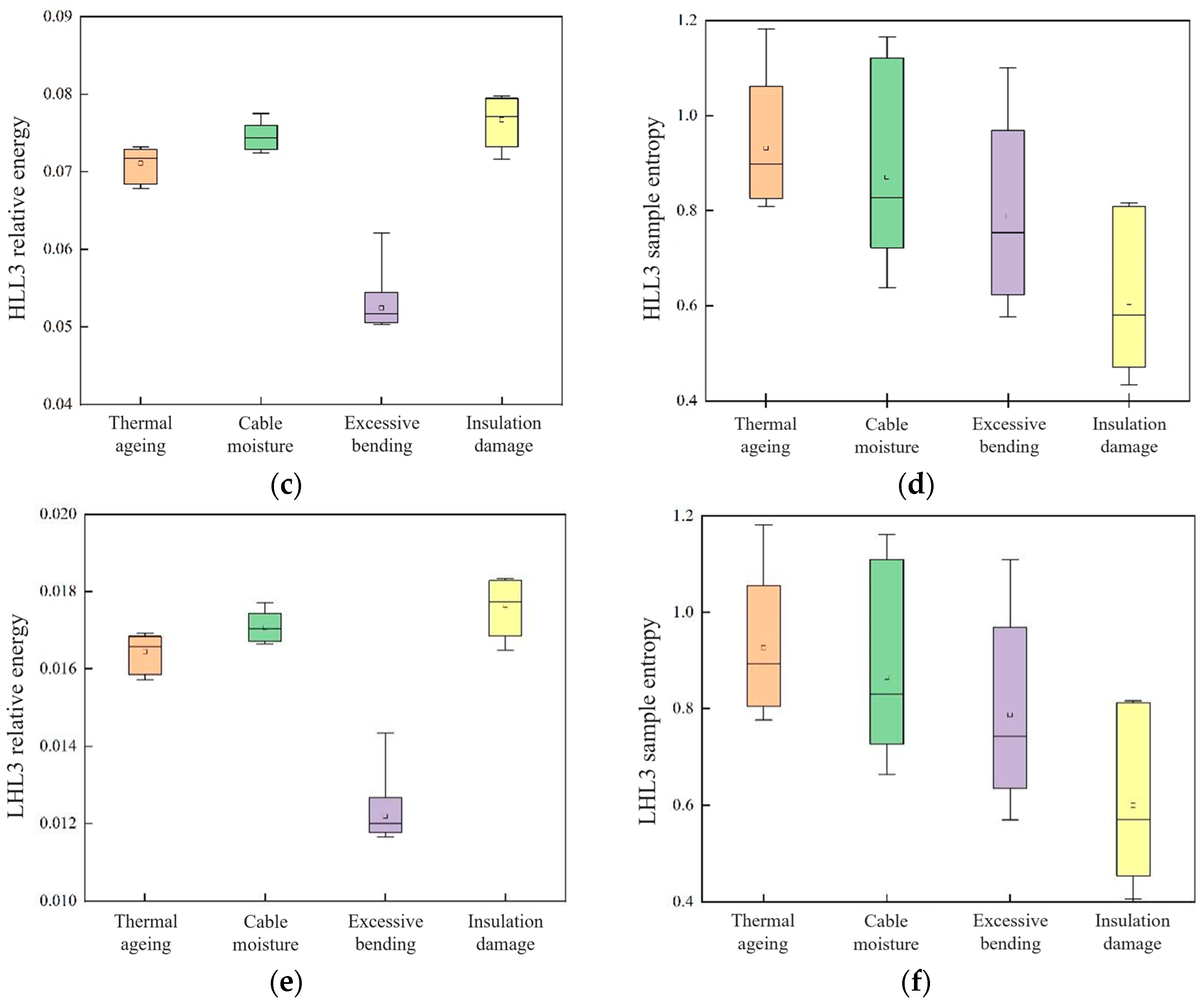
Figure 8.
The flow of the optimized model based on SSA-SVM.
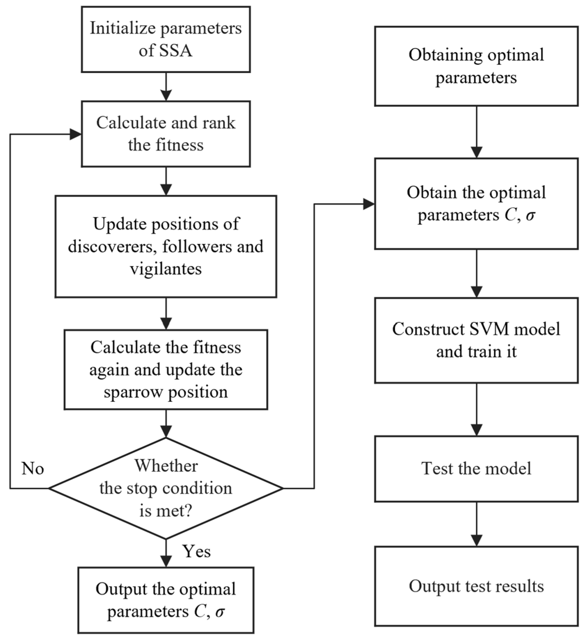
Figure 9.
The fitness change curve of the SSA-SVM model.
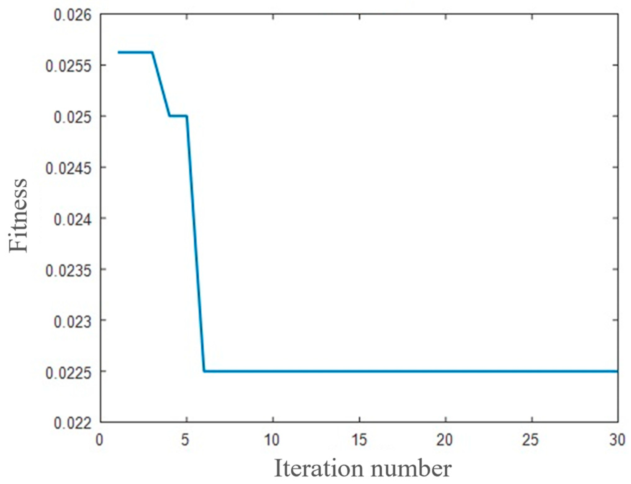
Figure 10.
The recognition results of the SSA-SVM. (a) Comparison of forecast and actual values; (b) Test Data Confusion Matrix;.
Figure 10.
The recognition results of the SSA-SVM. (a) Comparison of forecast and actual values; (b) Test Data Confusion Matrix;.
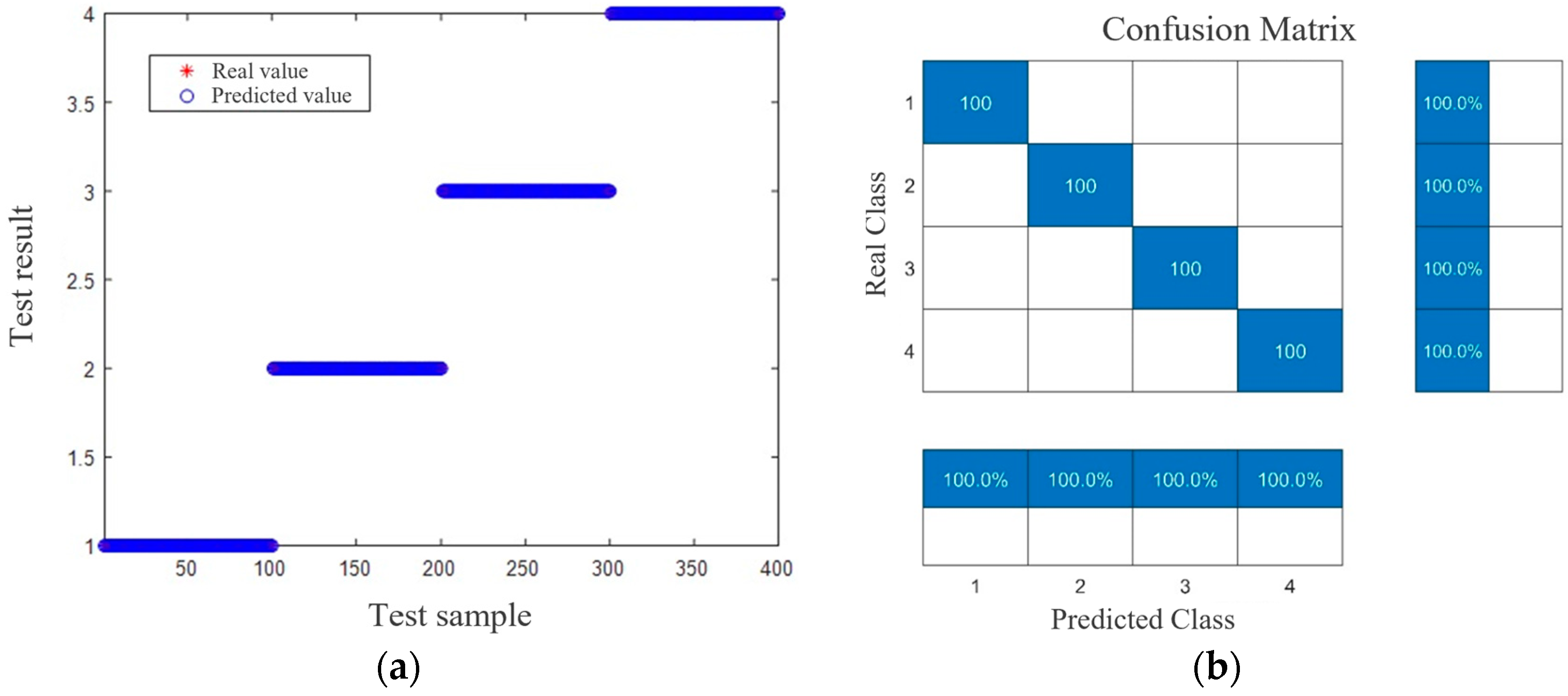

Table 1.
Simulation methods of typical defects.
| Defect Type | Simulation Method |
|---|---|
| Thermal ageing | Use the HK-450A+ electrothermal constant temperature oven to accelerate thermal ageing. Put the specimen into the oven after the temperature reaches 120℃. The sampling time is selected in an equal progression (12, 24 and 48 days) according to IEC 60811. |
| Cable moisture | Strip the outer sheath of the specimen, seal it with a heat-shrink sleeve filled with water and test it at 5, 10 and 15 days. |
| Excessive bending | Fixe the specimen to the wooden board using cable clamps and hexagonal screws according to the bending radius (R=600 mm, R=400 mm, R=200 mm), corresponding to the specimen length of 2 m, 1.6 m and 1.2 m. |
| Insulation damage | Peel off the outer sheath, metal shield and insulating shield sequentially at the middle section of the specimen, with a length of 40 mm. Construct the scratch on the insulating layer to set three levels of damage respectively, 40mm2mm1mm, 40mm4mm1mm, and 40mm6mm 1mm. |
Table 2.
Models and parameters of each equipment component.
| Equipment | Model/Parameter | Equipment | Model/Parameter |
|---|---|---|---|
| Regulator | TDGC2-3, CHNT | High-frequency Acquisition Card | PCI-1712, 20kHz |
| Test Transformer | TDM 11,000 kVA | Cable Specimen | YJLV8.7/15 kV-1×70 mm2 |
| Voltage Divider | RCF-50 kV | Protective Resistor | 1MΩ |
| Oscilloscope | MSO5104, RIGOL | Sampling Resistor | 10kΩ |
Table 3.
The formulae of time-domain features and frequency-domain features.
| Category | Calculation Formula | ||||
|---|---|---|---|---|---|
| Time-domain features | Mean | Skewness | |||
| Variance | Cliffiness | ||||
| Square root magnitude | Peak Factor | ||||
| Absolute Mean Magnitude | Waveform Factor | ||||
| Maximum | Impulse Factor | ||||
| Minimum | Margin factor | ||||
| Peak-to-peak | Skew factor | ||||
| Root-Mean- Square |
Cliff factor | ||||
|
Frequency-domain features |
Power Spectrum Mean | ||||
| Centre-of-gravity frequency | |||||
| Frequency Variance | |||||
| Frequency standard deviation | |||||
| Mean Square Frequency | |||||
| Root-mean-square Frequency | |||||
Table 4.
The parameter settings of SSA.
| Parameter | Setting |
|---|---|
| Number of sparrow groups | 10 |
| Maximum number of iterations | 30 |
| ST safety threshold | 0.7 |
| Proportion of discoverers | 40% |
| Proportion of vigilantes | 20% |
Table 5.
Method comparison.
| Comparison Items | SVM | BPNN | SSA-SVM | |||
|---|---|---|---|---|---|---|
| Before PCA | After PCA | Before PCA | After PCA | Before PCA | After PCA | |
| Recognition rate/% | 93.75 | 95.25 | 92.5 | 98.5 | 97.75 | 100 |
| Time consumption/s | 0.8961 | 0.4233 | 3.6536 | 0.8614 | 53.8151 | 23.9943 |
Disclaimer/Publisher’s Note: The statements, opinions and data contained in all publications are solely those of the individual author(s) and contributor(s) and not of MDPI and/or the editor(s). MDPI and/or the editor(s) disclaim responsibility for any injury to people or property resulting from any ideas, methods, instructions or products referred to in the content. |
© 2024 by the authors. Licensee MDPI, Basel, Switzerland. This article is an open access article distributed under the terms and conditions of the Creative Commons Attribution (CC BY) license (http://creativecommons.org/licenses/by/4.0/).
Copyright: This open access article is published under a Creative Commons CC BY 4.0 license, which permit the free download, distribution, and reuse, provided that the author and preprint are cited in any reuse.


