
Submitted:
14 April 2025
Posted:
15 April 2025
You are already at the latest version
Abstract
To solve the problem in which the vibration signal of the transformer is affected by noise and electromagnetic interference, which leads to the low accuracy of fault diagnosis pattern recognition. A CEEMDAN-MRAL fault diagnosis method based on Fiber Bragg grating (FBG) is proposed to evaluate the vibration fault state of the transformer quickly and accurately. The FBG sends the wavelength change of the optical signal center caused by the vibration of the transformer to the demodulation system, which obtains the vibration signal and effectively avoids the noise influence caused by strong electromagnetic interference inside the transformer. The vibration signal is decomposed into several intrinsic mode functions (IMFs) by complete ensemble empirical mode decomposition with adaptive noise(CEEMDAN), and the wavelet threshold denoising algorithm improves the signal-to-noise ratio (SNR) to 1.6 times. The Markov transition field (MTF) is used to construct a training and test set. The unique MRAL-Net is proposed to extract the spatial features of the signal and analyze the time series dependence of the features to improve the richness of the signal feature scale. This proposed method effectively removes the noise interference. The average accuracy of fault diagnosis of the transformer winding core reaches 97.9375%, and the time taken on the large-scale complex training set is only 1705s, which has higher diagnostic accuracy and shorter training time than other models.
Keywords:
FBG
; denoising algorithm
; CNN
; fault diagnosis
1. Introduction
Transformers are responsible for voltage conversion and power transfer. Their stability is crucial to the security and reliability of the power system. In long-term operation, transformers are affected by electrical, mechanical, and environmental factors, which may lead to faults such as loose windings and iron cores [1]. These may result in power outages and production interruptions, and in serious cases, they may even lead to safety accidents [2].
As an effective transformer fault diagnosis method [3,4], the vibration analysis method can reflect the local faults of transformer windings and cores.FBG accelerometer has excellent anti-electromagnetic interference ability and insulation effect, can still work stably for a long time in harsh environments, has high sensitivity and broadband response ability, can carry out multi-division multiplexing and high-precision distributed monitoring of transformer vibration signals in real time, and eliminates manual maintenance costs, and is suitable for the detection of transformer vibration signals. Vibration analysis based on FBG mainly includes signal preprocessing and fault diagnosis algorithms. In the aspect of signal preprocessing, time-frequency conversion methods such as short-time Fourier transform (STFT)[5], empirical mode decomposition (EMD)[6], wavelet transform (WT)[7] and variational mode decomposition (VMD) [8] can directly analyze the frequency and amplitude information of the signal. Still, these methods usually lose some time-domain information. Because the transformer may be affected by many uncertain factors in operation, the vibration signal characteristics are easily buried[9], so it is necessary to adopt appropriate denoising methods to improve the SNR to ensure that the amplitude-frequency characteristics of the signal can be better displayed, and provide support for the follow-up fault diagnosis model. Common denoising methods include wavelet threshold denoising, EMD denoising, and convolutional neural network denoising [10,11,12]. Still, these methods can only denoise the signal as a whole, so it’s tough to achieve targeted denoising.
Deep learning and machine learning methods are widely used in mechanical fault identification. Fang Liu improved the recognition accuracy of intrusion vibration signals by combining the Gaussian mixture model with the hidden Markov model, but the model is complex [13]. Alireza Shamlou et al.. use the time-frequency image generated by the Hilbert-Huang transform to input the classifier based on evidence theory. Although the frequency domain features are effectively utilized, a large amount of redundant information may be generated under the influence of noise, which makes it difficult to divide the decision boundary [14]. Convolution neural network (CNN) has become a popular method of transformer fault diagnosis because of its advantages in image recognition. The IP-CNN proposed by Huan Wu et al. improves the accuracy of fault identification through its powerful spectral time domain feature-learning ability [15]. Jing Cheng et al. achieved a classification accuracy of 97.1% by converting vibration signals into grayscale images combined with SVM and ResNet-18 but had limitations in high-dimensional feature processing [16]. Hao Wei et al. proposed a framework combining ResNet and an extreme learning machine, which uses continuous wavelet transform to enhance the performance of diagnosis, but the robustness of the model is poor [17]. Meng Chang et al. proposed an improved CNN combined with a convolutional attention mechanism to enhance the model diagnosis ability and reduce the complexity of the network, but the depth is not enough, and the effect of feature extraction is not good [18]. Rui Xiao et al. convert time series signals into images and improve the model robustness through semi-supervised learning, but may fall into the local optimal solution [19]. Rafia Nishat Toma et al.. improve signal quality and fault feature identification by ensemble empirical mode decomposition (EEMD) and continuous wavelet transform, but they still need to improve mode aliasing, computational complexity, and time-frequency resolution [20].
To sum up, to decrease the influence of noise and boost the accuracy of fault diagnosis, the CEEMDAN-MRAL transformer vibration signal fault diagnosis method based on FBG is proposed to identify transformer winding and core loose faults. The fault diagnosis scheme includes the following steps: firstly, the FBG accelerometer collects the change in the wavelength of the light wave center caused by the vibration of the fuel tank surface and converts it into a vibration signal through the demodulation system, CEEMDAN decomposes the signal into IMFs, screens the IMFs with sample entropy and other parameters, denoises the wavelet threshold for the IMF with high eigenity, and reconstructs to improve the signal-to-noise ratio. Secondly, MTF transform is used to transform a time series signal into an image, and the data set is constructed. Finally, the unique hybrid residual attention structure in the MRAL-Net model extracts the multi-scale structural features of the image, and the attention mechanism is used to recalibrate these features. The long short-term memory network(LSTM) carries on the time series analysis of the extracted features and sends them to the classifier for classification. Finally, the feasibility of this method is verified by experiments.
2. Basic Theories and Sensing Systems
2.1. Vibration Mechanism of the Transformer
The vibration of the winding and the iron core causes the vibration of the transformer shell, and the winding and the iron core can be regarded as a parallel subsystem, and the magnetostrictive phenomenon of the silicon steel sheet and the collision with each other causes the vibration of the iron core, and its vibration acceleration can be expressed as follow[21]:
L represents the length of the iron core, εs represents the magnetostriction of the iron core when the core is saturated, Us represents the amplitude of the sinusoidal voltage, N is the number of turns of the winding, s is the cross-sectional area of the iron core, the magnetic induction intensity of the Bs core is saturated, and w represents the frequency. The acceleration of the core vibration is proportional to the square of the voltage, and the frequency is twice the voltage frequency. When the winding coil passes through the sinusoidal current, the coil will be subjected to electromagnetic force because of the magnetic leakage flux, and the force of the winding can be analyzed as follows; each winding can be regarded as a mass block with a mass of M. the winding is often wrapped by a layer of insulating paper and separated by a splint, so the relationship between the groups can be seen as a combination of damping and elasticity, and the force analysis of the windings is shown in Figure 1, and the displacements are shown follows[22]:
where [M], [C], and [K] represent the matrices of mass, viscous damping, and stiffness coefficients, respectively. [F] represents the electromagnetic force vector matrix, and {x} represents the displacement vector. The acceleration of the winding is proportional to the square of the load current, and its frequency is also twice the frequency of the power supply [23], as shown below:
2.2. FBG Acceleration Sensing Principle
The principle of FBG (Fiber Bragg Grating) acceleration sensing is based on the wavelength coordination effect of FBG and the sensitivity of the internal mechanical structure to acceleration, and the strain caused by acceleration is converted into wavelength change for measurement, and only light that satisfies the Bragg condition will be reflected in FBG, as shown in equation (4), when subjected to strain or temperature change, the relationship between wavelength shift and strain and temperature is as follows equation (5), where λB is the reflected wavelength, neff is the effective refractive index of the fiber, Λ is the grating period, △λ is the wavelength change, △T is the temperature change, ε is the strain change, Pe is the photo elastic coefficient, α is the thermal expansion coefficient, and ξ is the thermo-optical coefficient.
The FBG accelerometer converts the acceleration into the axial strain of the FBG by the displacement of the cantilever beam and mass, as shown in Figure 2, and then demodulates the acceleration value by the wavelength offset. The acceleration a is given by equation (6-8); where L is the distance from the fixed end of the cantilever beam to the FBG connection point, E is the Young’s modulus, b, h is the width and thickness of the cantilever beam, and m is the mass of the mass.
2.3. FBG Sensing Systems
Considering that the working environment of the transformer is affected by electromagnetic interference, the vibration signal on the front of the transformer shell is measured by using the FBG accelerometer combined with the demodulation system, and the acceleration signal is obtained by feeling the change of the central wavelength of the reflected light, such as equation 8.
Figure 3 shows the signal acquisition system. The light signal emitted by the narrow-linewidth laser (NLL) is modulated into a pulse signal by the pulse generator(PG) and the electro-optic modulator (EOM). After being amplified by the erbium-doped fiber amplifier (EDFA), it is divided into six channels through an optical coupler and fed into the FBG accelerometer to detect the surface vibration signal of the transformer tank. The signal is sent to the photodetector (PD) through the circulator and is converted into an electrical signal. After the data acquisition card (DAQ) collects data, it is transmitted to the PC for processing and fault diagnosis. However, the collected signal is inevitably affected by uncertain factors, resulting in a large amount of noise or blurred amplitude and frequency characteristics, so subsequent signal preprocessing methods are required to denoise the signal and visualize the amplitude and frequency characteristics.
2.4. Pre-Processing of Transformer Vibration Signal
The vibration signal is collected based on FBG mainly contains sine and cosine signals with 100Hz as the fundamental frequency and its double frequency, but due to the influence of mechanical structure and current harmonics, it is often accompanied by a lot of noise, which can not effectively reflect the fault state of the winding and iron core. Therefore, it is necessary to denoise the vibration signal effectively. The pre-processing of signal consists of two parts: (1) denoising and reconstruction, that is, using CEEMDAN- wavelet threshold denoising algorithm, signals in different frequency ranges can be effectively separated, and the threshold is set by sample entropy, variance contribution rate, and correlation coefficient, to achieve a good denoising effect. (2) MTF image conversion: To highlight the amplitude-frequency characteristics of the signal, the convolution neural network is used to extract the spatial features of the denoised signal to transform it into an MTF image.
2.4.1. Denoising and Reconstruction
Compared with the traditional CEEMDAN reconstruction denoising and wavelet denoising methods, the CEEMDAN-wavelet threshold denoising algorithm can better adapt to the non-stationary characteristics of the signal, avoid the problem of aliasing, and improve the effect of signal denoising. Each IMF after denoising is reconstructed to get the denoising signal. The denoising process is as follows:
(1) CEEMDAN is used to decompose the signal into IMFs, each representing a different frequency component.
(2) The threshold is set by sample entropy, variance contribution rate, and correlation coefficient to retain the IMFs component, which is highly related to the original signal. The calculation formulas of sample entropy, variance contribution rate, and correlation coefficient are as follows:
In the formula, N represents the signal length, Ai represents the logarithm of similar subsequences, xi represents the signal before denoising, yi represents the processed signal, EV (xi) represents component variance, TV represents total variance, and N represents the signal length.
(3) Wavelet threshold denoising is applied to all reserved IMFs.
(4) The denoised IMFs are reconstructed to get the final denoised signal.
2.4.2. MTF Image Conversion
Markov transition field is a method that can chain the time series signal into the matrix. By mapping the values of each element in the matrix into pixels, the time series signal can be transformed into an image. The position of the pixel represents the time sequence, which effectively avoids the loss of time domain information.
First of all, the value of the given time series signal X={x1,x2,x3,...xn} is divided into Q discrete quantile units, and then the values in X are mapped to the corresponding Q to form Q={q1,q2,q3,...qn}, the transfer probability between the points is calculated according to the time axis order, the first-order Markov chain is obtained, and a matrix W of Q × Q is constructed, as shown below:
where wij represents the probability that qi is transferred to qj. However, the overall time domain information will be lost, so the Markov transfer field is introduced, and the matrix W is converted into the matrix M by converting the sequence of the amplitude axis to the time axis, as shown below:
where mij denotes the probability of the transfer of qi and qj on the matrix W. In this way, the information of the signal in the time domain is preserved, and the conversion of the time series signal to the image is completed by mapping the value on the matrix M into pixels. The overall signal preprocessing process is shown in Figure 4.
3. Fault Diagnosis Scheme
The proposed CEEMDAN- MRAL fault diagnosis scheme is shown in Figure 5. The training part is responsible for obtaining the optimal model of fault diagnosis, and the test part is used for pattern recognition of the test set to get four fault states. The fault diagnosis model includes a data preprocessing module and an MRAL-Net fault diagnosis module. For the collected signal, the data preprocessing module first improves the signal quality through CEEMDAN- wavelet threshold denoising, and then uses MTF transform to convert the denoised signal into an image. The MRAL-Net fault diagnosis model includes a mixed residual attention module (MRAM) and LSTM. MRAM extracts multi-scale spatial features of the image, and LSTM analyzes the time dependence of features to capture long-term dependencies.
In the part of data preprocessing, the CEEMDAN method decomposes the vibration signal into multiple IMF, calculates the sample entropy, variance contribution rate, and correlation coefficient of each component to screen the effective IMF component, and reconstructs the pure signal by wavelet soft threshold denoising. Then, MTF is used to convert the timing signal into an image, which is used as the input of the fault diagnosis module. MRAL-Net fault diagnosis module combines hybrid residual attention structure and LSTM. By introducing CBAM into the residual structure, the number of parameters is reduced, the key features are highlighted, redundant information is suppressed, the feature expression ability is strengthened, and the model is lighter and more efficient. The jump connection structure can effectively avoid over-fitting and alleviate the problems of gradient disappearance and explosion. On the other hand, LSTM enhances the memory ability of long-term sequence features and can adaptively and selectively remember important information. These designs make MRAL-Net have strong robustness and generalization ability.
3.1. Convolution Block Attention Module
The convolution block attention module (CBAM) is an efficient and lightweight attention mechanism that aims to improve the image processing performance of a convolution neural network (CNN). The CBAM in Figure 6 consists of a channel attention module (CAM) and a spatial attention module (SAM). CAM obtains a 1 × 1 feature vector through maximum pooling and average pooling, calculates the weight coefficient of each channel through a multi-layer perceptron and Sigmoid activation function, and multiplies it with the input feature to get the output feature. SAM pays attention to spatial information, takes the output of CAM as input, generates a spatial attention map through pooling and convolution operation, and multiplies it with input features after activation of the Sigmoid function to realize dynamic enhancement of the feature graph. In equation 14-15, Fc, Fs represents the output of CAM and SAM, MPL represents multi-layer perceptron, σ represents sigmoid activation function, Avgpool and Maxpool represent average pooling and maximum pooling operation, f represents input characteristic graph, W7 represents 7 × 7 convolution operation, [Avgpool (f); Maxpool (f)] represents splicing operation.
3.2. LSTM Time-Dependent Analysis
LSTM solves the problem of gradient disappearance by introducing a memory unit and gating mechanism to learn long-term dependency. As shown in Figure 7, each LSTM unit includes a memory unit, an input gate, a forgetting gate, and an output gate. The input gate decides to update the stored information, the forgetting gate controls which information is discarded, and the output is determined according to the current input and storage information. The mathematical representation of LSTM is as follows.
where x represents the input of t time, h represents the output of t time, c represents the memory information of t time, o represents the output of the door, f and i represent the output of the forgetting gate and input gate, respectively, and b is the corresponding bias coefficient.
3.3. Mixed Residual Attention Structure
The residual neural network solves the problem of decreasing feature extraction ability with the increase of network depth through the residual structure, and its core idea is to stack the input and output characteristic graphs to alleviate the network degradation. To reduce the network depth while ensuring an excellent feature extraction effect, two hybrid attention residual structures are proposed (Figure 9). In the traditional residual structure (Figure 8), residual block 1 uses two 3 × 3 convolution layers, each convolution layer is followed by batch normalization and ReLU activation function to propagate information; residual block 2 adjusts the size of the input feature map through 1 × 1 convolution to make it consistent with the 3 × 3 convolution feature map, and then add them.
The hybrid residual attention structure proposed in this paper combines global pooling, convolution, and full join operations to calculate attention weights, reduce computational complexity, and ensure performance. After batch normalization, the channel attention mechanism and spatial attention mechanism are added in turn, and finally, the output is added to the 3 × 3 convolution input. If the input and output dimensions are different, 1 × 1 convolution is used to adjust the input size to ensure that the features are not lost. For the formulas of mixed residual structures 1 and 2, see (21-22). Relu represents the activation function, Fc and Fs represent CAM and SAM, respectively, BN represents batch normalization calculation, wi is convolution calculation, x represents input, and y represents output.
Among them, the batch normalization layer (BN) can make the network training more stable and fast, reduce the setting requirements of network parameters, reduce the overfitting of the network, and improve the generalization and robustness of the model. The batch normalization process is shown as follows:
3.4. MRAL-Net Model
The MRAL-Net model proposed in this paper includes a 7 × 7 convolution layer, a CBAM module, a maximum pooling layer, 8 mixed residual attention structures, an average pooling layer, a flattening layer, an LSTM layer, and a linear connection layer. The network structure is shown in Figure 10. The specific parameters are shown in Table 1. The model uses a 224x224 three-channel MTF image as input, and the specific structure is as follows: the first layer is 7 × 7 convolution, which is used to extract global features, the second layer is the CBAM module, which enhances important features and suppresses redundancy, and the third layer is 3 × 3 maximum pool, which reduces the dimension of features and reduces the amount of computation. Layers 4 to 7 form Residual Block (a), which extracts deep features through the residual structure to solve the problems of gradient disappearance and explosion, in which Residual1 is repeated twice, Residual2 and 3 are repeated once, and each residual block contains a set of 3 × 3 convolution and batch normalization. The 8th to 11th layers are mixed residual attention structure group Residual Block (b), which further extracts image features, reduces redundancy, and improves computational efficiency. Residual4 and Residual6 adopt hybrid structure 2 and Residual7 adopt hybrid structure 1; layer 12 is the average pooling layer, which further reduces dimension and retains local features; layer 13 is flattening layer, which converts features into 1-dimensional vectors for input LSTM The 14th and 15th layers are the LSTM layer, and the hidden state dimension is 128, which is used for time series feature analysis, and the 16th layer is the linear layer, which outputs 4 classification results.
4. Experimental Setup
The sensor is fixed at the oil tank 1/6 and 5/6 of a 110kv oil-immersed transformer to collect vibration signals. The transformer type is SZ10-31500/110, and the rated voltage is 110kv ±8 × 1.25% /10.5. The sampling frequency is set to 10kHZ, and the vibration signal of 1s is collected. The vibration signals of normal, loose winding, and loose iron core are shown in Figure 11. In the normal state, the main frequency of the vibration signal is 100HZ, and the content of high-order harmonics is less. When the winding is loose, the content of 300-600HZ increases significantly, and the amplitude of the 100HZ component decreases by about 30%. When the core is loose, the amplitude of the 200HZ component increases significantly and contains a small amount of 400HZ-900HZ components.
In the signal preprocessing stage, the noise standard deviation of the CEEMDAN process is set to 0.2,60 times of noise addition, and the maximum number of iterations is 100. In the process of wavelet denoising, db5 is used as the wavelet basis function, the soft thresholding method is used, and the number of decomposition layers is set to 2. The denoised vibration signals are converted into MTF images by the MTF method for every 1000 sampling points. A total of 8800 images, 2200 of each type, are generated, which are divided into training sets, validation sets, and test sets, as seen in Table 2. The input size of the image is 224 × 224 pixels, and the random horizontal flip is carried out to increase the data diversity and improve the generalization ability of the model. 32 pictures were used in each training, the training process lasted 50 times, and the initial learning rate was 0.0001.
In this paper, precision, recall, F1 score, and accuracy are used to evaluate the classification effect of the model on the test set. Precision represents the proportion of samples that the model predicts to be positive and that is positive, and the higher the precision is, the less the false prediction is negative class. Recall refers to the proportion in which the model is correctly predicted to be positive in all the positive samples. The higher the recall rate, the more positive samples can be identified by the model. The F1 score is the harmonic average of accuracy and recall. Considering the performance of both, the higher the F1 score is, the better the model is in terms of accuracy and coverage. Accuracy is the proportion of the number of samples identified correctly out of the total sample. The calculation formula for each index is as follows:
In the formula, TP, FP, FN, and TN represent the number of samples with correct predictions as positive, false predictions as positive, incorrect predictions as negative, and correct predictions as negative, respectively. To verify the effectiveness of the denoising method in this paper, noise is added to the signal, and the denoising effect is evaluated by using the SNR, root mean square error (RMSE), correlation coefficient (CC), and roughness (R). The formula is as follows (31-33). For the calculation formula of the correlation coefficient, see 16. The larger the SNR, the lower the RMSE, and the closer CC and R are to 1, the better the denoising effect is, and the smoother and undistorted the signal is. In the formula, x(t) is the signal before denoising, y(t) is the processed signal, and N represents the signal length.
5. Experimental Results and Discussion
5.1. Verification of Denoising Effect
Taking the normal signal as an example, the time domain maps of 10 IMF components and residual components are obtained by CEEMDAN decomposition, as shown in Figure 12. The high-frequency component is mainly concentrated in IMF1-IMF4, which contains a lot of noise; IMF5 and IMF6 are relatively stable and have large amplitudes, and the energy is mainly concentrated in these two components, which belong to the dominant component of the signal; IMF7-IMF10 has low frequency and small amplitude, so it belongs to low-frequency noise. Table 3 lists the comparison parameters for each IMF. Line chart 13 shows the changing trend of each parameter. IMF1 and IMF2 have high entropy, high complexity, and uncertainty, which are mainly noise components; the variance contribution rates of IMF3 and IMF5 are 0.3065 and 0.5652 respectively, indicating that their variance accounts for a large proportion; the correlation coefficients of IMF3, IMF4, and IMF5 are 0.586, 0.3916 and 0.7481, respectively, indicating a high correlation with the original signal, representing the amplitude and frequency characteristics of the signal.
To screen the effective IMF components and obtain the reconstructed signal with a high SNR, we add 10dB noise to the original signal and decompose it by CEEMDAN to get multiple IMF components. Calculate the SNR, RMSE, CC, and R values for the different IMF component reconstructions, as shown in Figure 14, after the wavelet threshold denoising reconstruction of the residual component and IMF3 and its subsequent IMF components, the highest SNR reaches 16.5794, the lowest RMSE is 0.1774, and the values of CC and R are 0.9892 and 1.048 respectively, which is the closest to 1, it indicates that the denoised signal obtained by preserving IMF3 and its subsequent components has the highest SNR, has a strong correlation with the original signal and the signal is the smoothest.
Wavelet threshold denoising [24] and CEEMDAN reconstruction denoising [25] are excellent signal denoising methods, which are compared with the proposed methods in this paper. Figure 15 shows the results of denoising normal vibration signals under the SNR of 5 dB, 10 dB, and 15 dB. Under different SNRs, the method used in this paper improves the SNR of 6.5160db, 6.5794db, and 6.2508db; RMSE reached 0.3178, 0.1774, and 0.1011; CC is 0.9667, 0.9892 and 0.9964; R values are 1.1523, 1.0480 and 1.0081, each value reaches the optimal value in different conditions and different methods, SNR promotion is the highest, RMESE is the lowest, CC and R-value are approximately 1, indicating that the signal quality after denoising is the best and the correlation and roughness with the original signal is fabulous. The waterfall diagram of the denoising effect of the three methods on the normal vibration signal at 10db SNR is shown in Figure 16. The signal processed by this method is smoother and shows better signal smoothing ability and denoising performance. This method is not only more robust and has the ability of multi-scale analysis but also can deal with complex signals more effectively and significantly improve the signal quality combined with wavelet threshold denoising.
Because the data set used in this paper is a two-dimensional image rather than a one-dimensional time series signal, to verify the effectiveness of the proposed denoising method on MTF images, Figure 17 shows the MTF images without and after CEEMDAN- wavelet threshold denoising. The results show that the CEEMDAN-wavelet threshold denoising method can effectively eliminate noise interference, significantly reduce image noise, retain the main features, ensure that the signal quality is not affected, highlight the frequency and amplitude characteristics of the signal after denoising, and provide a reliable guarantee for follow-up fault diagnosis.
5.2. Verification of Training Effect
Figure 18 shows the loss and accuracy curves of the MRAL-Net, ResNet-18, GoogLeNet, AlexNet, and LeNet network models. All models use the same MTF image data set, learning rate, cross-entropy loss function, and Adam optimizer to evaluate the performance difference. From the training accuracy curve, we can see that all models achieve good convergence, among which MRAL-Net has the fastest convergence speed, and the accuracy remains stable and high after convergence. GoogLeNet can extract multi-scale features based on its Inception module, but the accuracy fluctuates greatly after convergence. AlexNet converges slowly, and its accuracy fluctuates slightly, while LeNet converges slowest, and training accuracy is the lowest. From the validation accuracy curve, while the training accuracy of MRAL-Net is improved, the validation accuracy is gradually increasing and tends to be stable. In contrast, ResNet-18 fluctuates between 30 and 35 epochs, while the accuracy of other models fluctuates greatly. Generally speaking, MRAL-Net performs best, which verifies its superiority in MTF image analysis after denoising.
Figure 19 shows the box plot of the accuracy and loss rate of training and validation for 20 iterations after each model is stable. The upper and lower boundaries of the box are the upper quartile and the lower quartile. The flatter the box is, the smaller the fluctuation is, and the better the convergence is. The larger the median line and average value of the accuracy rate are, the smaller the median line and average value of the loss rate are, which means the higher the accuracy of fault diagnosis of the model. MRAL-Net has the smallest quartile spacing, the least outlier samples, the highest accuracy median line and average, and the lowest loss rate median line and average value, indicating that its iterative process is the most stable and convergent, and it can accurately learn and predict the samples in the data set. Table 4 shows that among the stable accuracy and loss rates of each model, the average accuracy of MRAL-Net in the training set and validation set is 0.9986 and 0.9764, respectively, which is significantly better than that of LeNet, which is 0.0427 and 0.0315 higher than that of LeNet. At the same time, the loss rate is the lowest, only 0.0041 and 0.1157; the training loss rate is 0.1080 lower than LeNet, and the validation loss rate is 0.1467 lower than AlexNet. Table 5 shows the time consumption of each model in 50 iterations. MRAL-Net takes only 1705 seconds, which is 187 seconds less than lightweight ResNet-18 and 441 seconds less than GoogLeNet. These results show that MRAL-Net shows excellent performance in terms of accuracy, loss rate, and computing time.
Evaluate the performance of the model by confusion matrix on the test set, and calculate the precision, recall, F1 score, and overall accuracy, as shown in Table 6. 0, 1, 2, 3 represent the normal state, the core is loose, the winding is loose, and both the winding and the core are loose. The classification precision is 1, 0.9674, 0.9852, and 0.9646, respectively, for the normal state, the core is loose, the winding is loose, and there are samples with both the core and the winding being loose. The recall rates were 1, 0.9650, 1, and 0.9525, respectively. F1 scores were 1, 0.9662, 0.9925, and 0.9585, respectively, for the normal samples, the MRAL-Net classification is completely correct; for the loose core samples, 14 are misjudged as the winding and the iron cores are loose; all the winding loose samples are classified correctly, among the samples with loose windings and iron cores, 13 were misjudged as only the iron core was loose, and 6 were misjudged as winding looseness. The misjudgment is mainly focused on the type where both the windings and the core are loose because the obvious vibration signal characteristics mask the weak features, resulting in the classification bias to prominent fault features. Despite this, the overall accuracy of the test set is 97.9375%, and the classification performance of normal, loose core, and loose winding samples is excellent, which fully verifies the excellent performance of MRAL-Net.
To evaluate the performance of the proposed model on the test set, we compare it with four classical networks: ResNet-18, GoogLeNet, AlexNet, and LeNet, and calculate the average precision, recall, and F1 score, retaining four decimal places. The results are shown in Table 7. As can be seen from the table, MRAL-Net performs best in all three indicators, reaching 0.9830, 0.9794, and 0.9812, respectively. Compared with LeNet, these three indicators are improved by 0.0406, 0.0413, and 0.0410, respectively, which fully reflects the excellent performance of MRAL-Net in fault diagnosis. For four kinds of fault diagnosis samples, MRAL-Net can accurately distinguish different categories, and there are few misjudgments. The average accuracy on the test set is shown in Figure 20. MRAL-Net is 0.0413 higher than LeNet and 0.0056 higher than ResNet-18, showing its highest accuracy in fault diagnosis tasks.
5.3. Ablation Experiment
To verify the effectiveness of each module for fault diagnosis, we designed four groups of ablation experiments: A is the model to remove LSTM, B is the model to remove CBAM, C is the model to replace the residual structure with the original residual structure, and D is the complete model. Each model was tested on 8 test sets, conducted a total of 32 experiments, and recorded the accuracy, as shown in Figure 21. The experimental results show that removing the key modules will significantly reduce the feature learning ability of the model. After removing CBAM or replacing residual structure, the feature extraction ability of the model decreases obviously, indicating that CBAM and mixed residual attention structure are effective in extracting fault information. In addition, when the LSTM layer is removed, the accuracy of fault diagnosis is also decreased, indicating that LSTM is very important for analyzing the timing dependence of features. The results show that these key modules play an important role in feature learning and fault diagnosis.
5.4. Comparison of Different Schemes
Short-time Fourier transform (STFT), Wavelet transform (WT), and Gramian angular difference field (GADF) are time-frequency analysis methods commonly used in mechanical fault diagnosis, which can convert one-dimensional time series signals into two-dimensional images. In this study, these four time-frequency analysis methods are combined with the MRAL-Net model and four classical network models: ResNet-18, GoogLeNet, AlexNet, and LeNet. In the experiment, we use the same parameters to train each model, compare the test on the same test set, and finally show the test accuracy through Figure 22. The results show that the combination of MRAL-Net and two-dimensional image conversion method is generally better than other combinations in accuracy, especially the combination of MRAL-Net and MTF, and the accuracy is 0.0606 higher than that of the combination of LeNet and STFT. The dataset generated based on MTF also performs better than the dataset generated by other methods.
The method of literature 17,18,22,25 is compared with the method proposed in this paper. Literature 17 combines a residual network with an extreme learning machine, literature 18 uses an improved residual network, Literature 22 uses a lightweight convolutional neural network, and literature 25 combines a convolutional neural network with a support vector machine. Table 8 shows four average indicators of the five methods, and the method proposed in this paper performs best in all kinds of indicators, which proves the excellent performance of this method.
6. Conclusions
In this paper, we propose a CEEMDAN-MRAL transformer vibration signal fault diagnosis method based on FBG, which can quickly and accurately identify different fault states of transformer cores and windings, CEEMDAN was used to decompose the vibration signal demodulated by the FBG sensing system into multiple IMFs, and the IMFs components were screened by sample entropy, variance contribution rate and correlation coefficient, effectively and finely removing instantaneous noise on different frequency components; the MRAL-Net model extracts the spatial scale characteristics of the vibration signal on the MTF image and analyzes the time-varying characteristics, to accurately learn the amplitude and frequency characteristics of the vibration signal of the transformer winding and the core. The unique mixed residual attention structure enables the model to quickly learn complex features while avoiding the problem of gradient vanishing and improving the robustness of training. The attention mechanism of the neck of the model further improves the attention to important features through the weighting of channel attention and spatial attention, and finally, the double-layer LSTM effectively retains the long-term memory of features and captures the temporal dependence of features. The experimental results show that the average accuracy of the scheme for the fault diagnosis of the transformer winding core reaches 97.9375%, and the accuracy of the fault diagnosis for normal and winding is 100%, which is better than that of other comparison methods. This scheme is also suitable for a variety of mechanical vibration fault diagnoses.
In future work, we will do more research on focused vibration signal noise processing and pattern recognition feature extraction to improve the accuracy of transformer fault diagnosis.
Funding
This work was supported in part by the Jilin Scientific and Technological Development Program Funding Project under Grants 20220203051SF.
References
- Z. Yuan, G. Sun, H. Tang, K. Gao, J. Hu, and J. He, “Types and Mechanisms of Condenser Transformer Bushing Failures,” in IEEE Electrical Insulation Magazine, vol. 39, no. 5, pp. 26-36, September/October 2023. [CrossRef]
- S.Tenbohlen, F. Vahidi and J. Jagers, “A Worldwide Transformer Reliability Survey,” VDE High Voltage Technology 2016; ETG-Symposium, Berlin, Germany, 2016, pp. 1-6.
- YongTeng Sun, HongZhong Ma, Research progress on oil-immersed transformer mechanical condition identification based on vibration signals, Renewable and Sustainable Energy Reviews, Volume 196,2024,114327, ISSN 1364-0321. [CrossRef]
- Hong Zhou, Kaixing Hong, Hai Huang, Jianping Zhou, Transformer winding fault detection by vibration analysis methods, Applied Acoustics, Volume 114,2016, Pages 136-146, ISSN 0003-682X. [CrossRef]
- Jian Zhao, Mingyu Chang, Yuqing Yang, Xutao Wang, Sheng Li, Tianhua Xu, Nonlinear impairment compensationin multi-channel communication systems based on correlated digital backpropagation with separation of walk-off effect, Optical Fiber Technology, Volume 86,2024,103850, ISSN 1068-5200. [CrossRef]
- Liu, X.; Tang, Y.; Zhang, Z.; Yang, S.; Hu, Z.; Xu, Y. A Pattern Recognition Method for Filter Bags in Bag Dust Collectors Based on Φ-Optical Time-Domain Reflectometry. Photonics 2024, 11, 152. [CrossRef]
- Sen Zhu, Yulin Wang, Yunfan Xu, Yuefeng Qi, Yanyan Liu, Fang Zhang, Asymmetric fiber grating overlapping spectrum demodulation technology based on convolutional network and wavelet transform noise reduction, Optical Fiber Technology, Volume 90,2025,104132, ISSN 1068-5200. [CrossRef]
- Bangning Mao, Zehua Bu, Ben Xu, Huaping Gong, Yi Li, Hailong Wang, Juan Kang, Shangzhong Jin, Chunliu Zhao, Denoising method based on VMD-PCC in φ-OTDR system, Optical Fiber Technology, Volume 74,2022,103081, ISSN 1068-5200. [CrossRef]
- YongTeng Sun, HongZhong Ma, Research progress on oil-immersed transformer mechanical condition identification based on vibration signals, Renewable and Sustainable Energy Reviews, Volume 196,2024,114327, ISSN 1364-0321. [CrossRef]
- Chen, Y.; Yu, K.; Wu, M.; Feng, L.; Zhang, Y.; Zhu, P.; Chen, W.; Hao, J. Wavelet Decomposition Layer Selection for the φ-OTDR Signal. Photonics 2024, 11, 137. [CrossRef]
- Shangze Chen, Xinglin Tong, Liwei Liu, Hongren Li, Xianyu Li,Vibration signal denoising algorithm based on corrosion detection of petroleum volatilization pipeline, Optical Fiber Technology, Volume 87,2024,103912, ISSN 1068-5200. [CrossRef]
- Hong Jiang, Rui Tang, Zepu Cao, Lina Cui, A small-sized fire detection method based on the combination of the SIC algorithm and 1-DCNN, Measurement, Volume 242, Part D,2025,116191, ISSN 0263-2241. [CrossRef]
- Fang Liu, Haiwen Zhang, Xiaorui Li, Zhengying Li, and Honghai Wang, “Intrusion identification using GMM-HMM for perimeter monitoring based on ultra-weak FBG arrays,” Opt. Express 30, 17307-17320 (2022). [CrossRef]
- Alireza Shamlou, Mohammad Reza Feyzi, Vahid Behjat, Winding deformation classification in a power transformer based on the time-frequency image of frequency response analysis using Hilbert-Huang transform and evidence theory, International Journal of Electrical Power & Energy Systems, Volume 129,2021,106854, ISSN 0142-0615. [CrossRef]
- Huan Wu, Bin Zhou, Kun Zhu, Chao Shang, Hwa-Yaw Tam, and Chao Lu, “Pattern recognition in distributed fiber-optic acoustic sensor using an intensity and phase stacked convolutional neural network with data augmentation,” Opt. Express 29, 3269-3283 (2021). [CrossRef]
- Jing Cheng, Qiuheng Song, Hekuo Peng, Jingwei Huang, Hongyan Wu, and Bo Jia, “Dual-model hybrid pattern recognition method based on a fiber optic line-based sensor with a large amount of data,” Opt. Express 30, 1818-1828 (2022). [CrossRef]
- Hao Wei, Qinghua Zhang, Minghu Shang, Yu Gu, Extreme learning Machine-based classifier for fault diagnosis of rotating Machinery using a residual network and continuous wavelet transform, Measurement, Volume 183,2021,109864, ISSN 0263-2241. [CrossRef]
- M. Chang, D. Yao, and J. Yang, “Intelligent Fault Diagnosis of Rolling Bearings Using Efficient and Lightweight ResNet Networks Based on an Attention Mechanism (September 2022),” in IEEE Sensors Journal, vol. 23, no. 9, pp. 9136-9145, 1 May 1, 2023. [CrossRef]
- R. Xiao, Z. Zhang, Y. Dan, Y. Yang, Z. Pan and J. Deng, “Multifeature Extraction and Semi-Supervised Deep Learning Scheme for State Diagnosis of Converter Transformer,” in IEEE Transactions on Instrumentation and Measurement, vol. 71, pp. 1-12, 2022, Art no. 2508512. [CrossRef]
- Nishat Toma, R.; Kim, C.-H.; Kim, J.-M. Bearing Fault Classification Using Ensemble Empirical Mode Decomposition and Convolutional Neural Network. Electronics 2021, 10, 1248. [CrossRef]
- Qiang H, Jingkai N, Songyang Z, et al. Study of transformer core vibration and noise generation mechanism induced by magnetostriction of grain-oriented silicon steel sheet[J]. Shock and vibration, 2021, 2021(1): 8850780. [CrossRef]
- K. Hong, M. Jin and H. Huang, “Transformer Winding Fault Diagnosis Using Vibration Image and Deep Learning,” in IEEE Transactions on Power Delivery, vol. 36, no. 2, pp. 676-685, April 2021. [CrossRef]
- Z. Xing et al., “Vibration-Signal-Based Deep Noisy Filtering Model for Online Transformer Diagnosis,” in IEEE Transactions on Industrial Informatics, vol. 19, no. 11, pp. 11239-11251, Nov. 2023. [CrossRef]
- Fuyu Wang, Jian Cen, Zongwei Yu, Shijun Deng, Guomin Zhang, Research on a hybrid model for cooling load prediction based on wavelet threshold denoising and deep learning: A study in China, Energy Reports, Volume 8,2022, Pages 10950-10962, ISSN 2352-4847. [CrossRef]
- Shi, L.; Liu, W.; You, D.; Yang, S. Rolling Bearing Fault Diagnosis Based on CEEMDAN and CNN-SVM. Appl. Sci. 2024, 14, 5847. [CrossRef]
Figure 1.
Winding force analysis diagram.
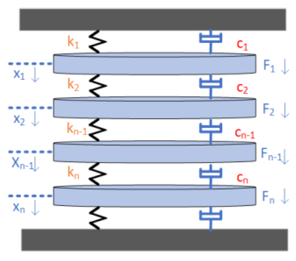
Figure 2.
FBG acceleration sensing schematic.
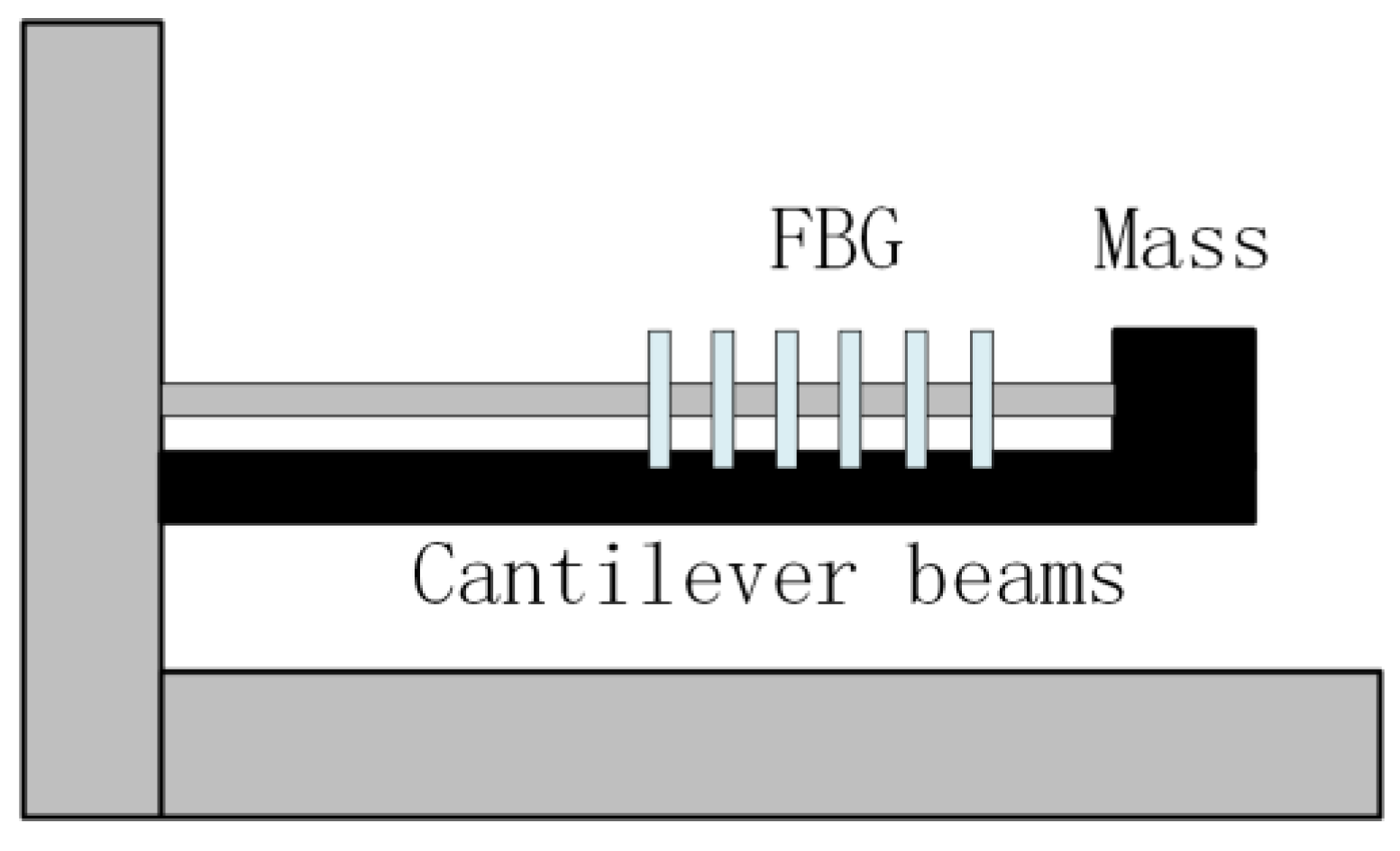
Figure 3.
Transformer vibration signal acquisition system based on FBG.
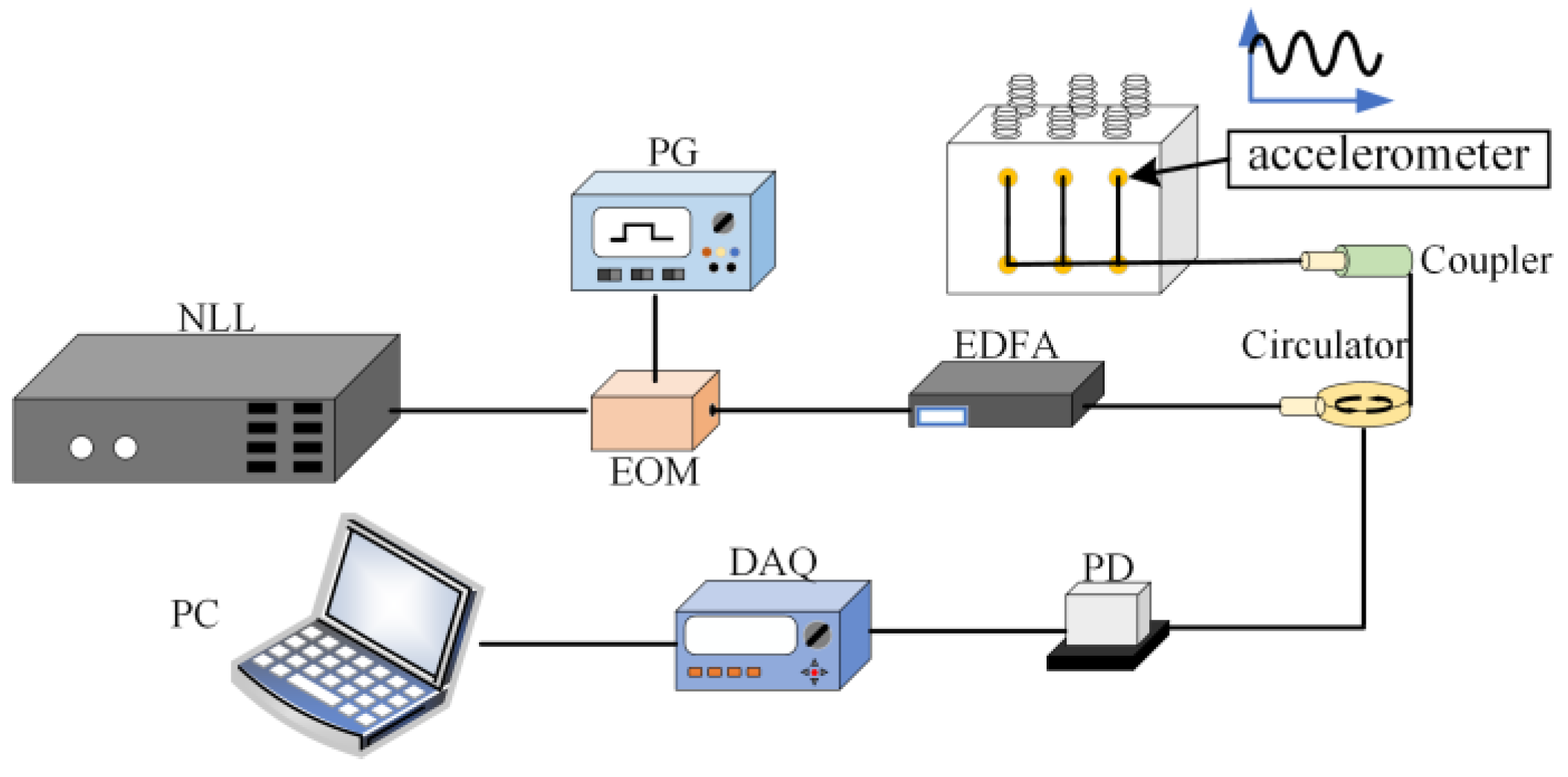
Figure 4.
Signal pre-processing process.
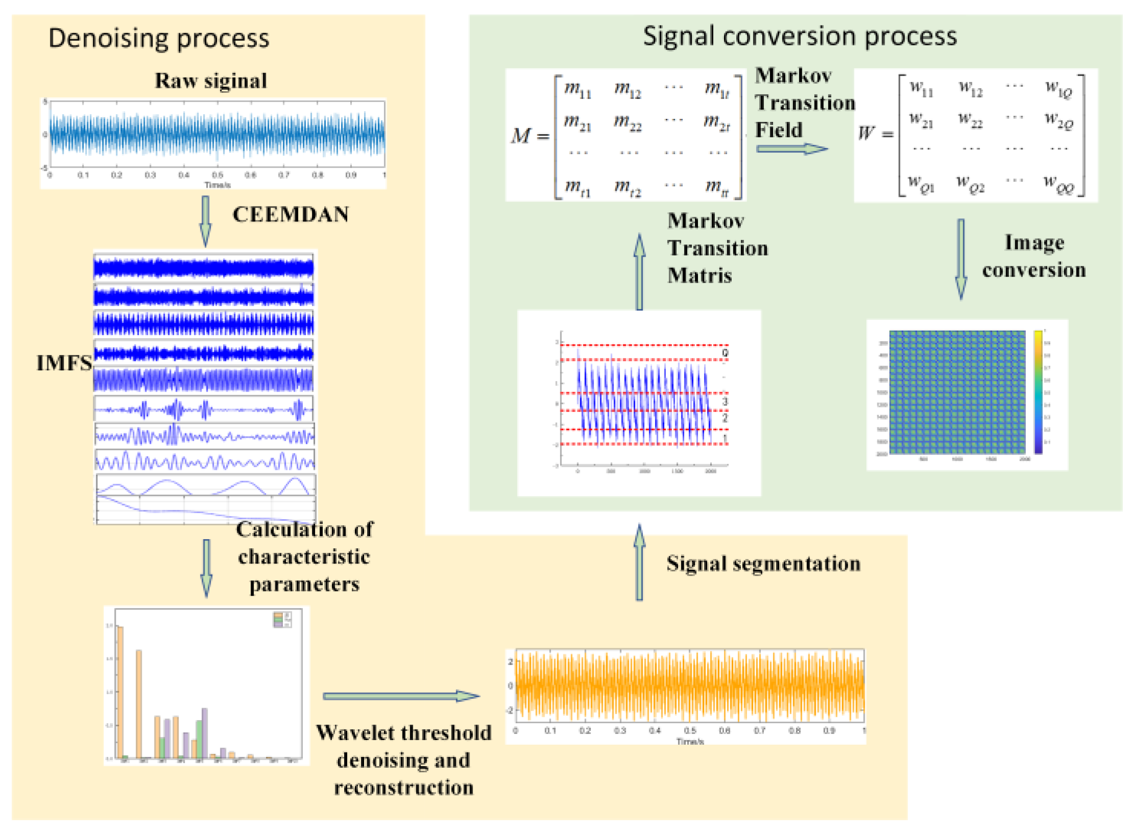
Figure 5.
CEEMDAN- MRAL fault diagnosis method.
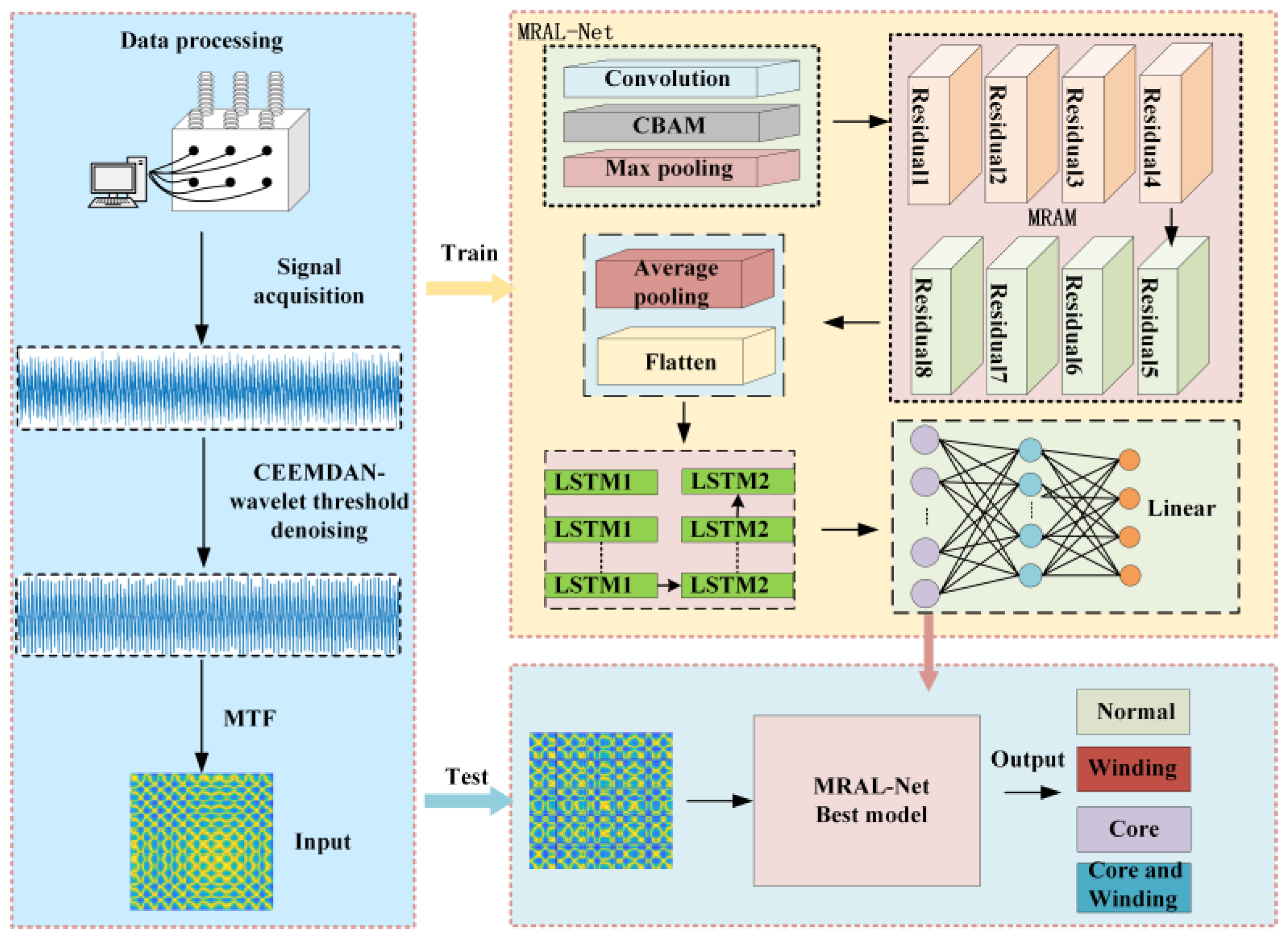
Figure 6.
Structure diagram of CBAM.
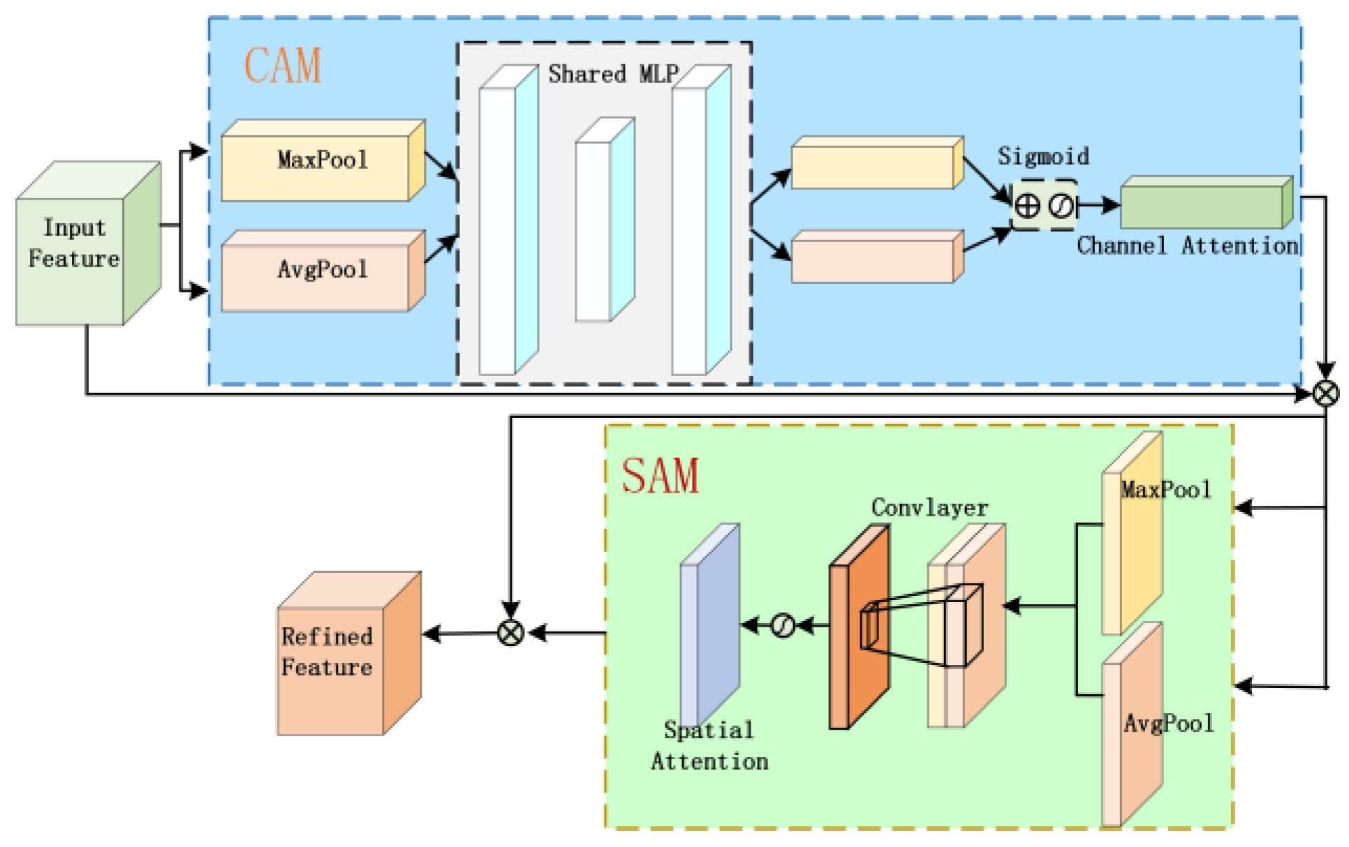
Figure 7.
LSTM structure diagram.
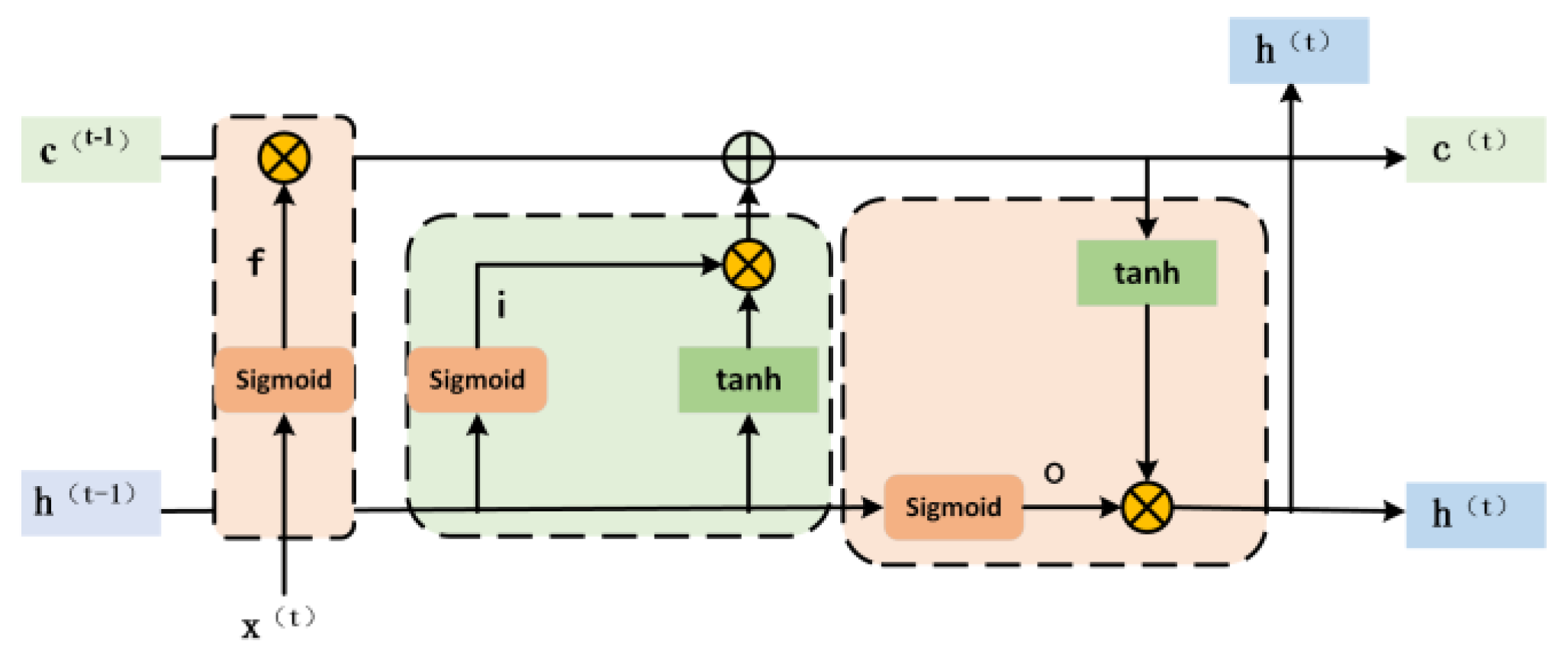
Figure 8.
Residual block 1 structure diagram a and residual block 2 structure diagram b.
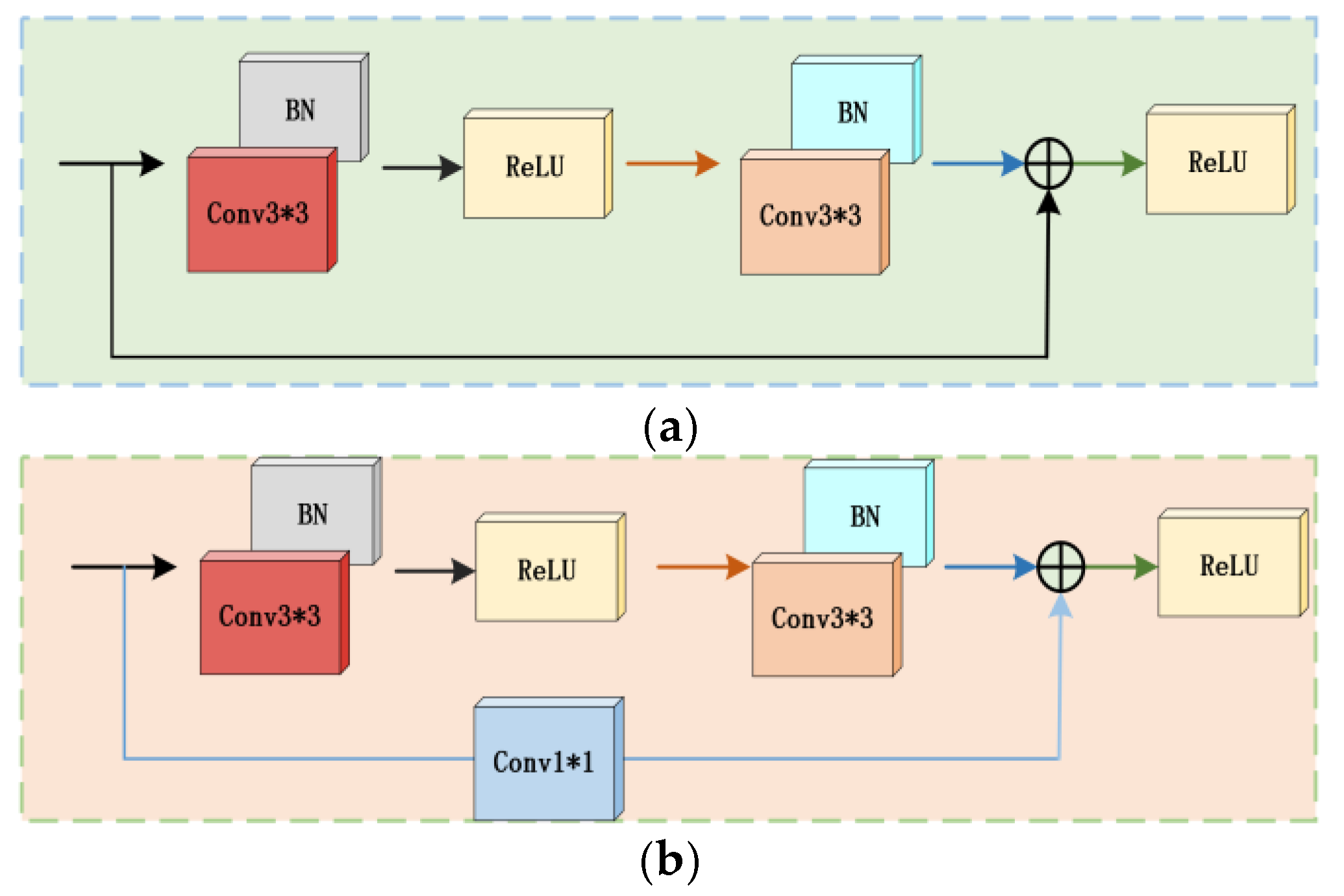
Figure 9.
Improved structure diagram of Residual Block 1 (a) and Residual Block 2 (b).
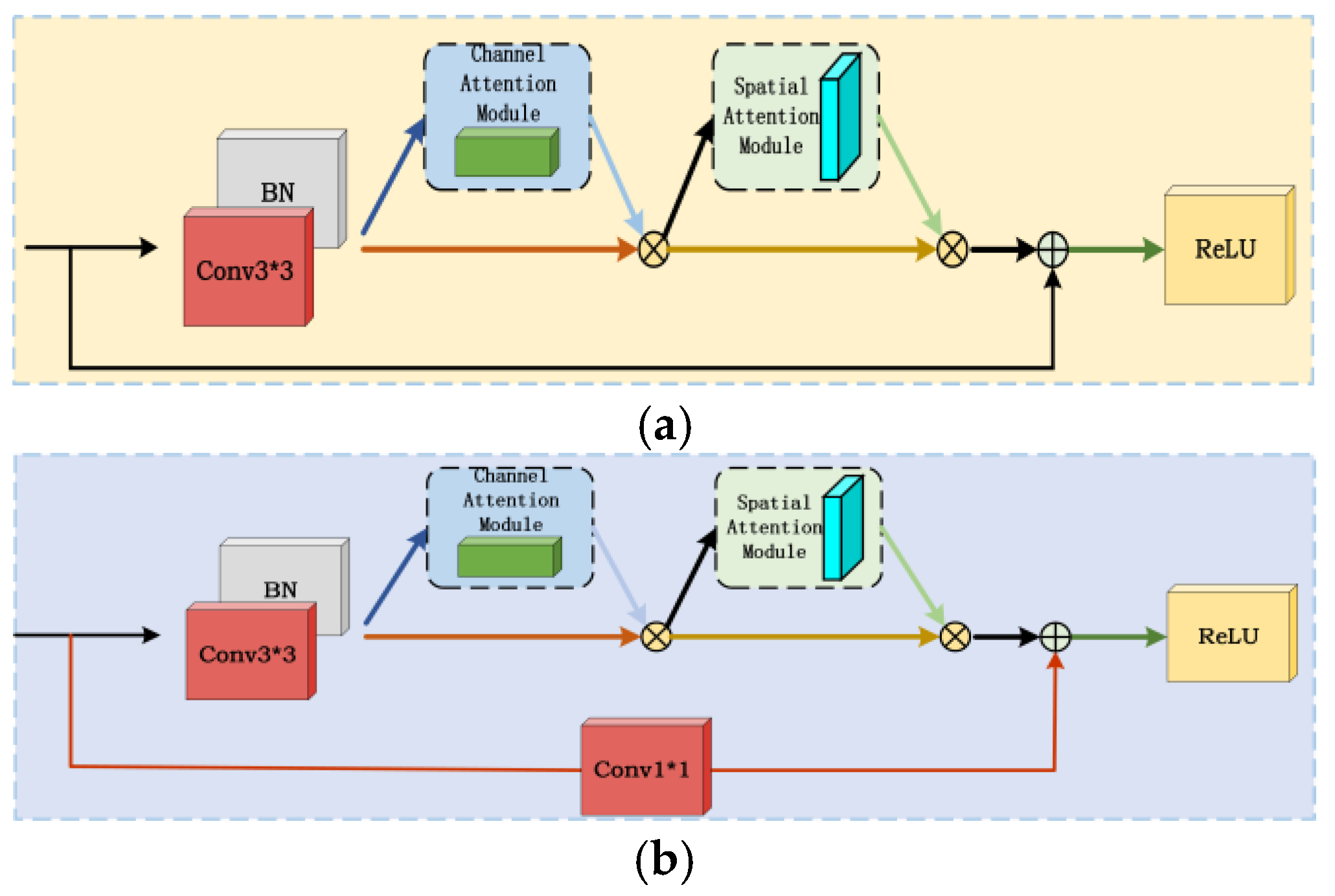
Figure 10.
MRAL-Net network architecture.

Figure 11.
a. Vibration in the time and frequency domains during normal time. b. Vibrating time- and frequency-domain signals when windings are loose. c. Vibration time and frequency domain signals when the core is loose. d. Vibration of time- and frequency-domain signals when the core and windings are loose.
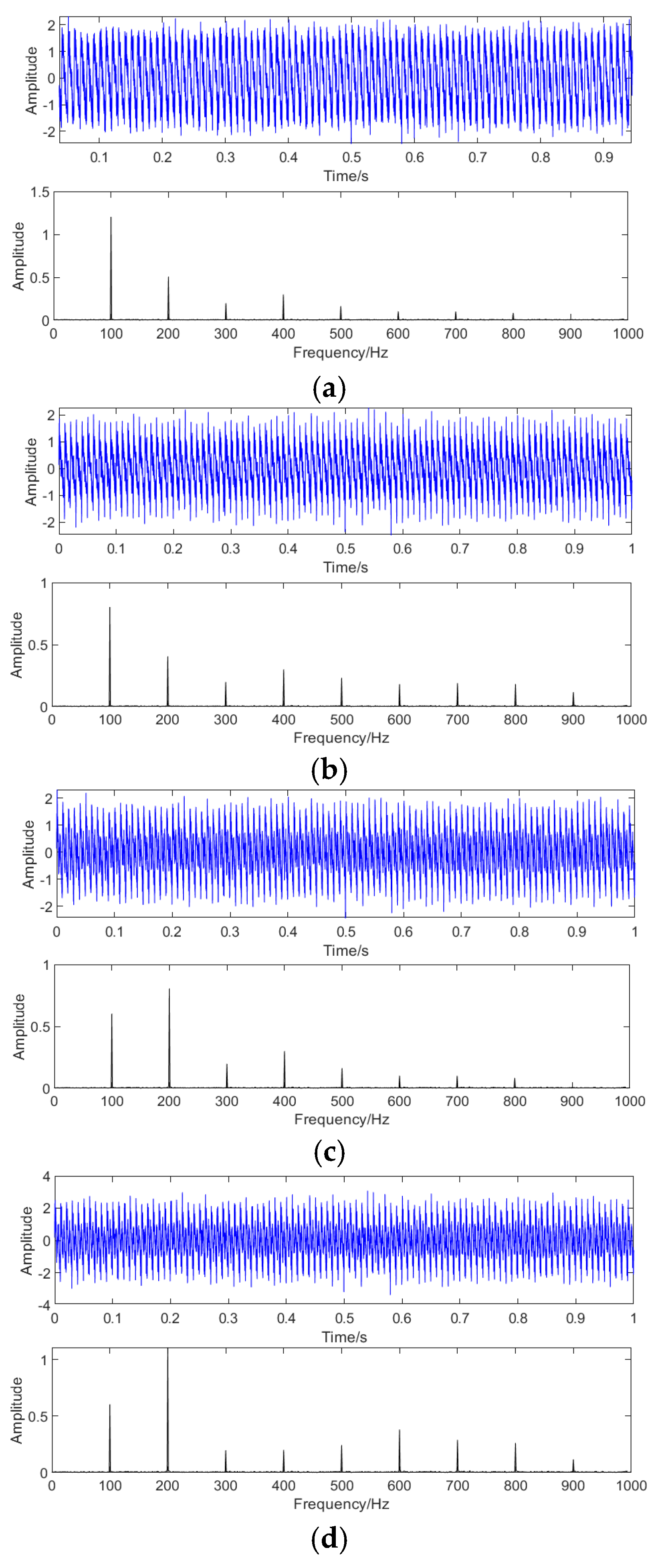
Figure 12.
IMFs obtained by normal signal decomposition.
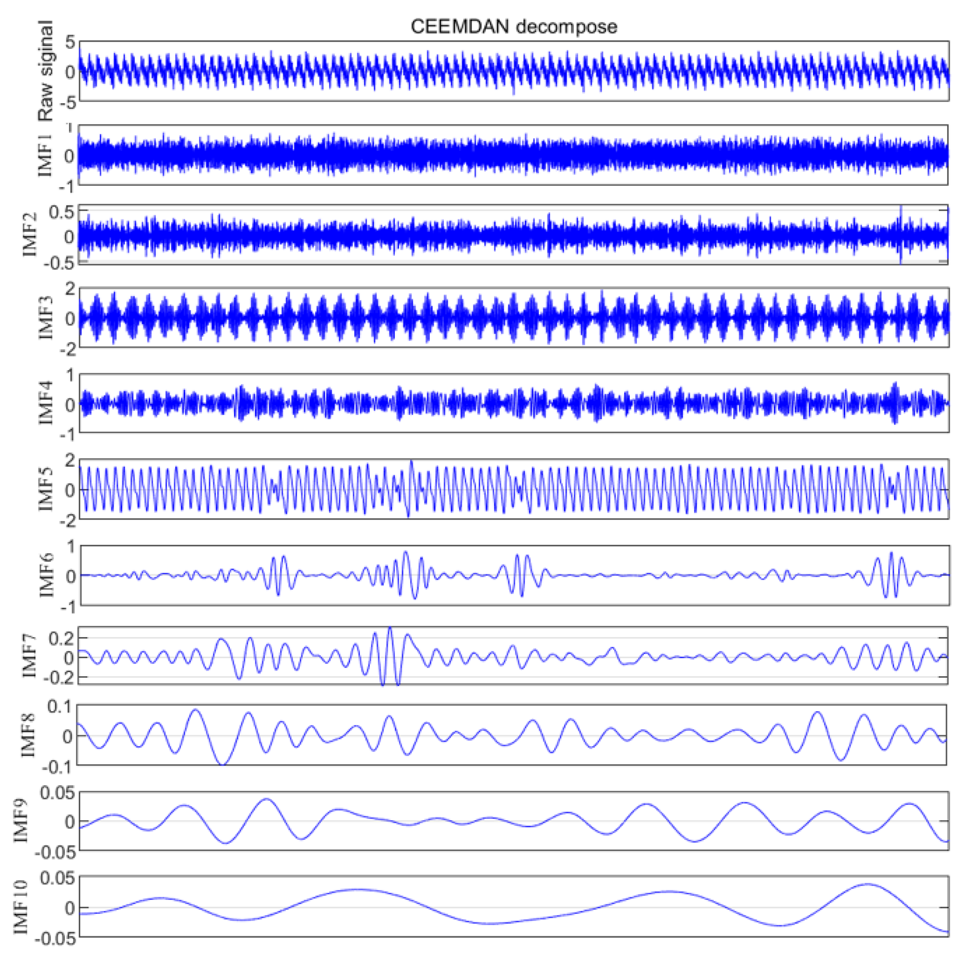
Figure 13.
Line chart of SE, VCR, and CC of each IMF component.
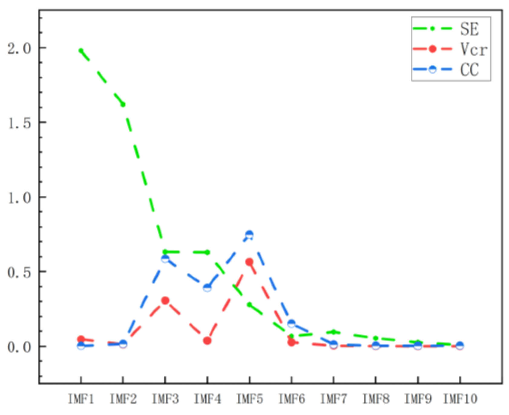
Figure 14.
The reconstructed SNR, RMSE, CC, and R of each IMF.
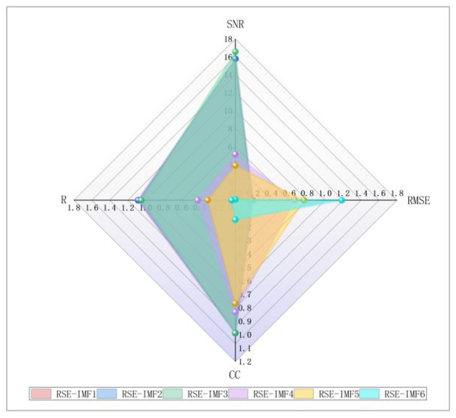
Figure 15.
SNR, RMSE, CC, and R at 5 db(a), 10 db(b), and 15 db(c).
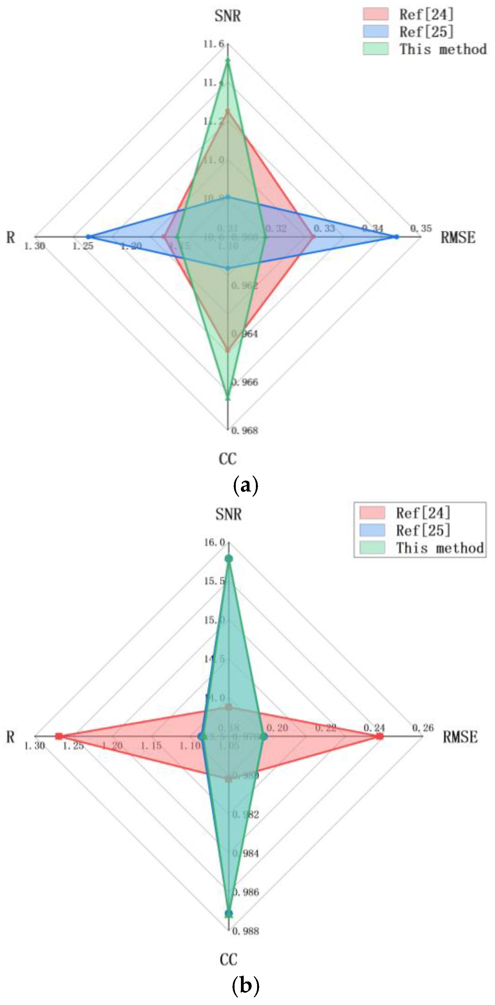
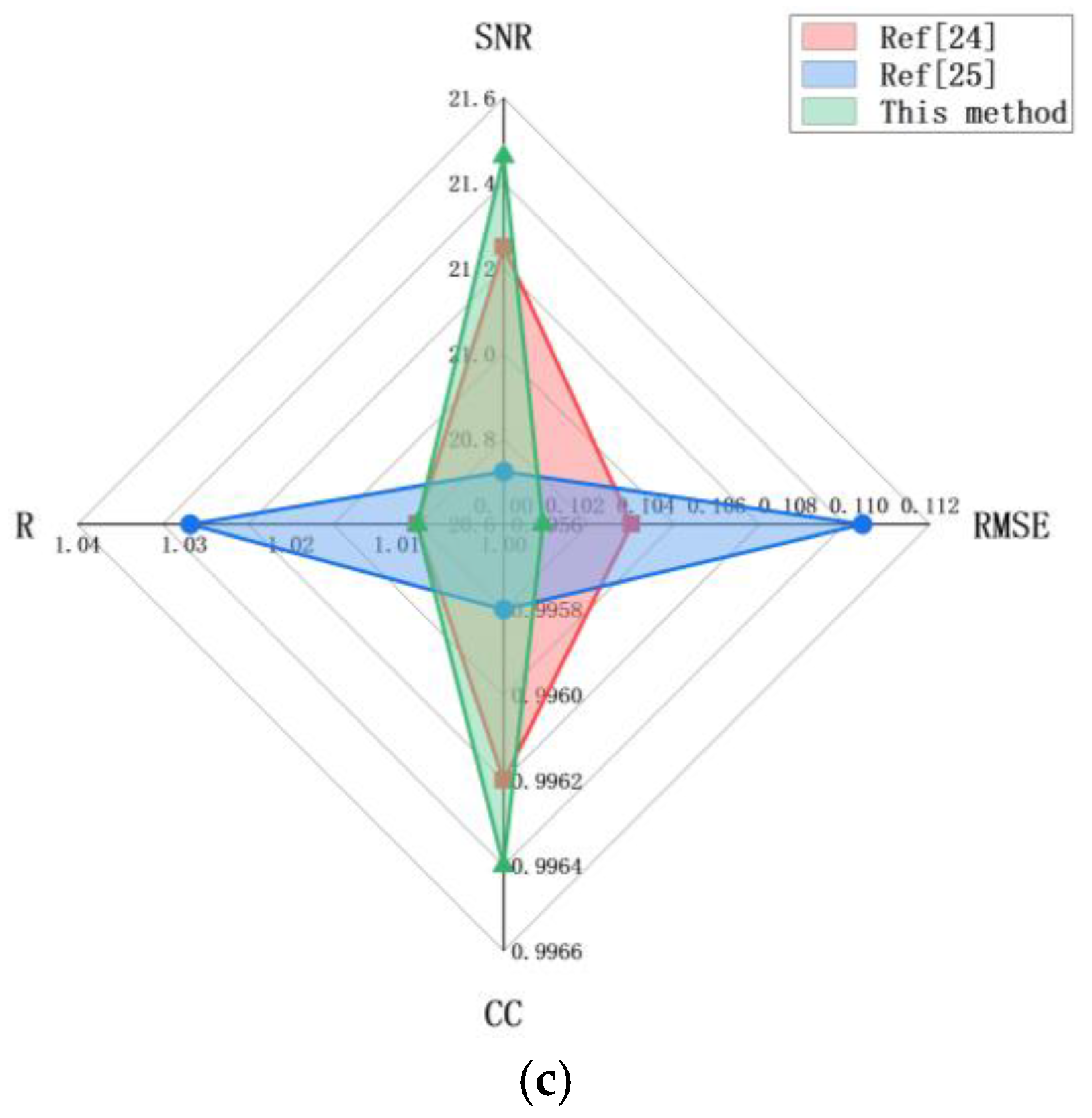
Figure 16.
Waterfall diagram of the denoising effect of the three methods.
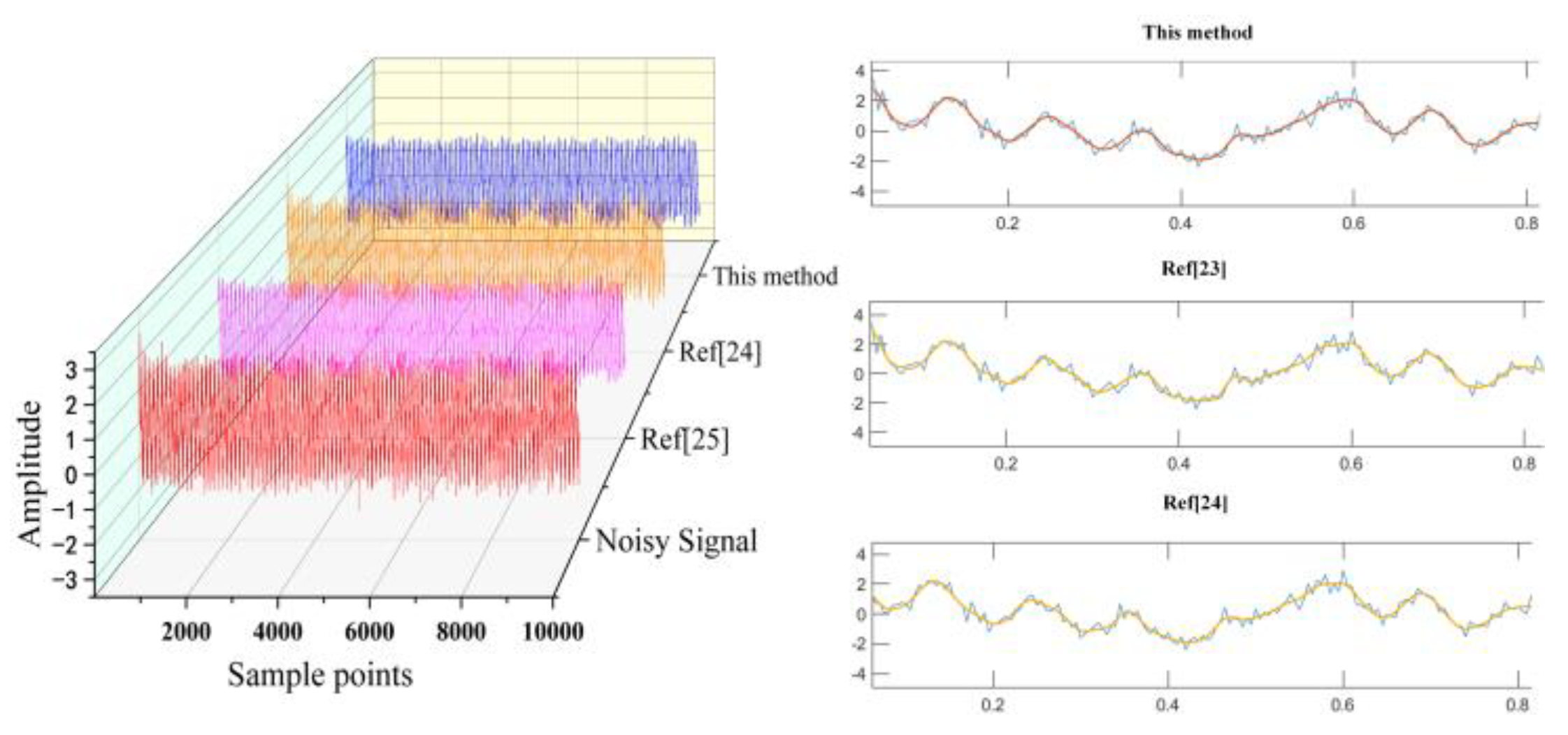
Figure 17.
Undenoised MTF image (a) and denoised MTF image (b).
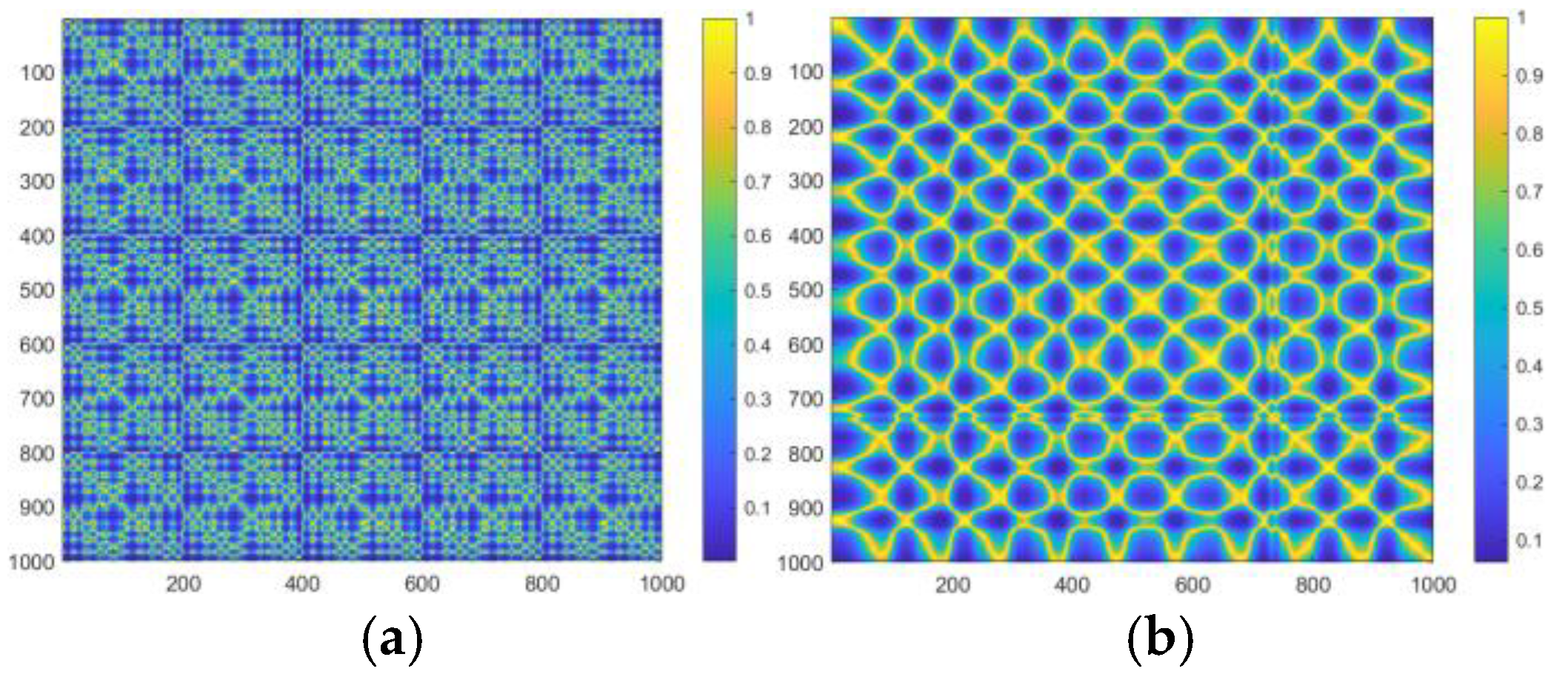
Figure 18.
(a) Accuracy of the training set, (b) loss rate of the training set, (c) accuracy of the validation set, and (d) loss rate of the validation set.
Figure 18.
(a) Accuracy of the training set, (b) loss rate of the training set, (c) accuracy of the validation set, and (d) loss rate of the validation set.
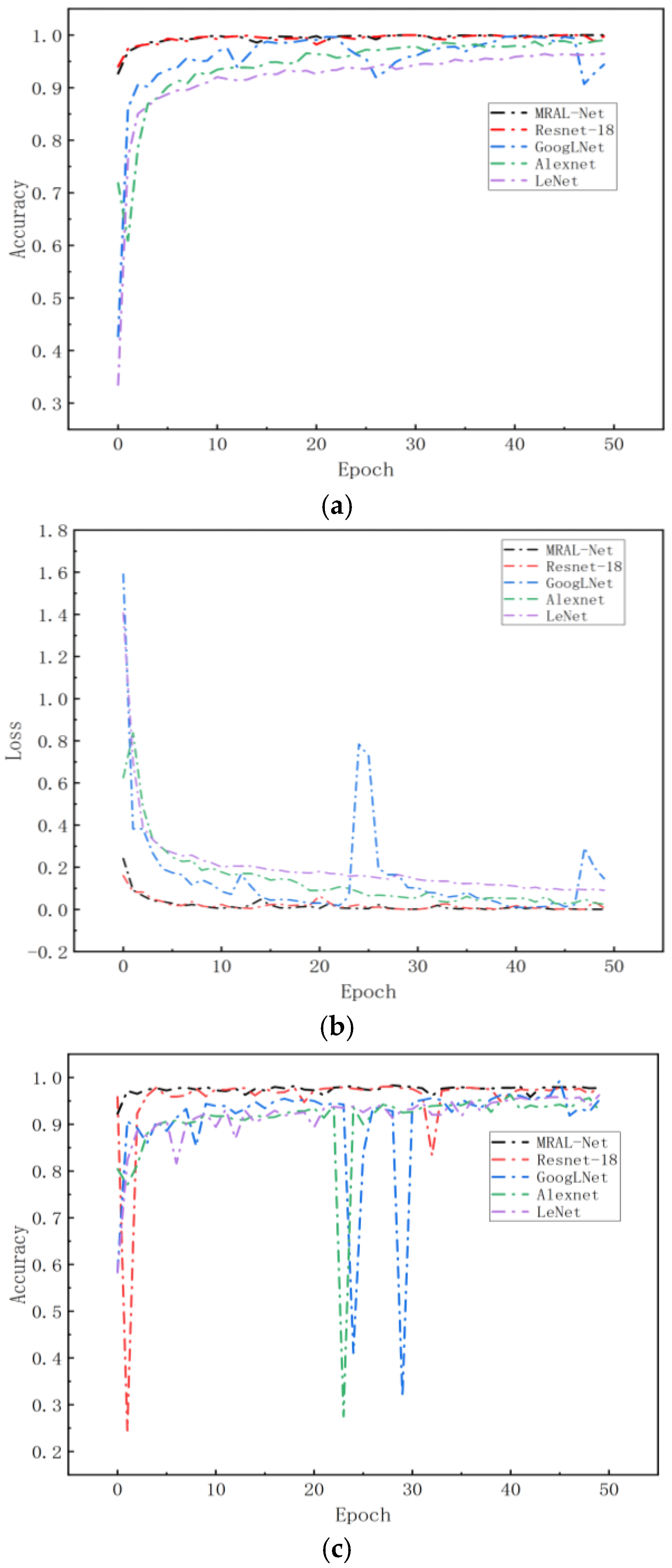
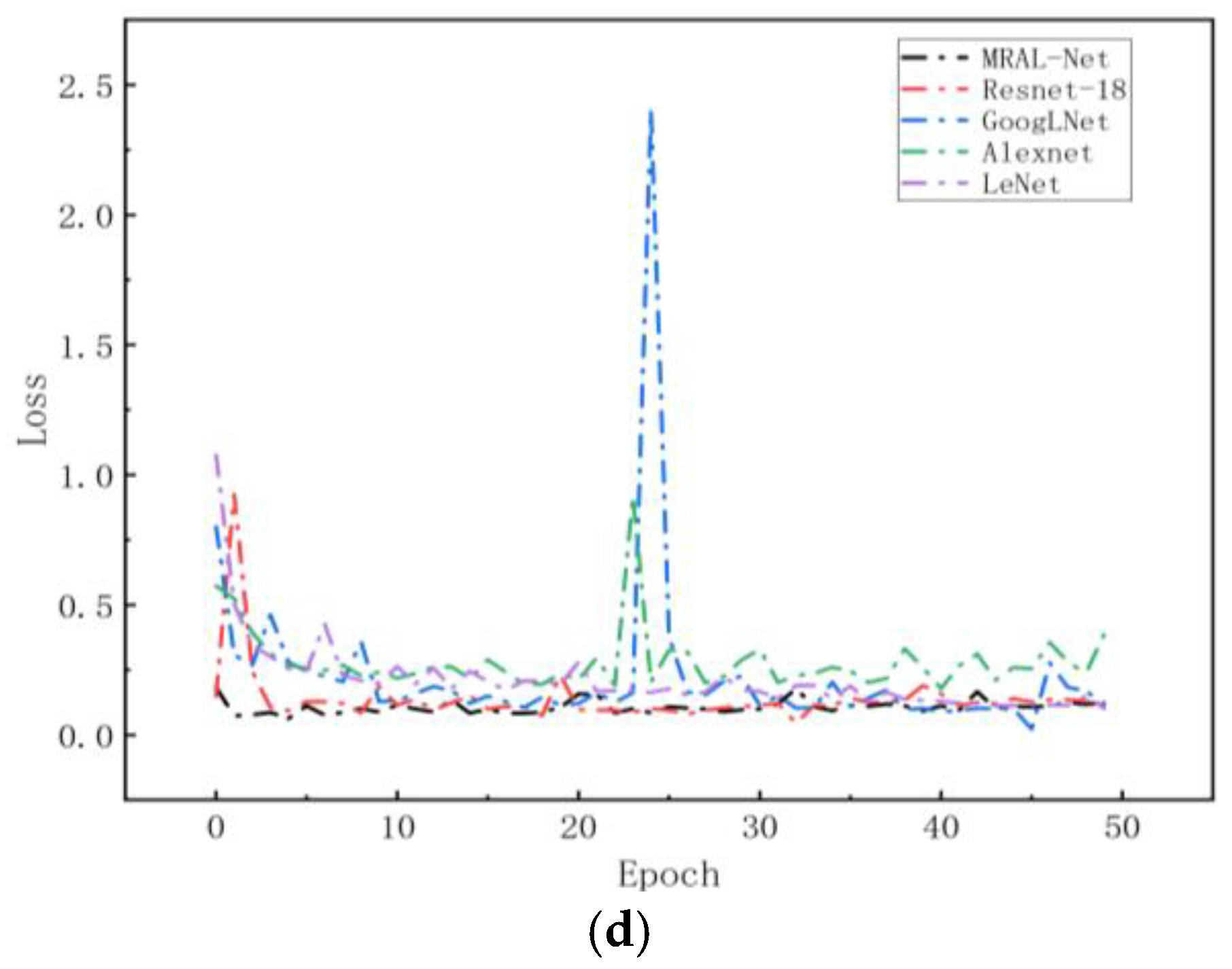
Figure 19.
Box plot of training and validation accuracy and loss rate.
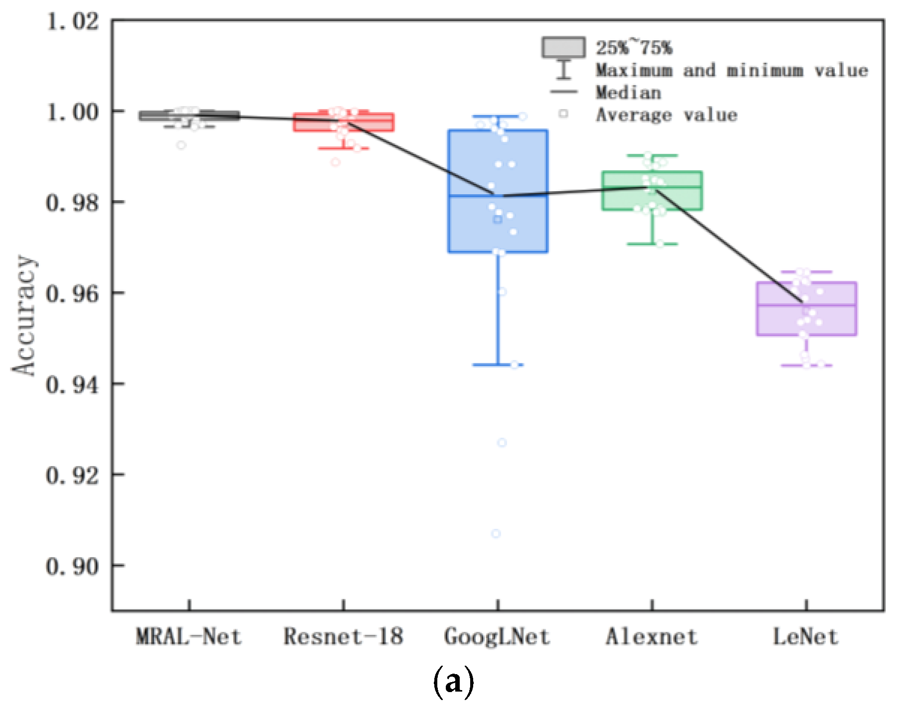
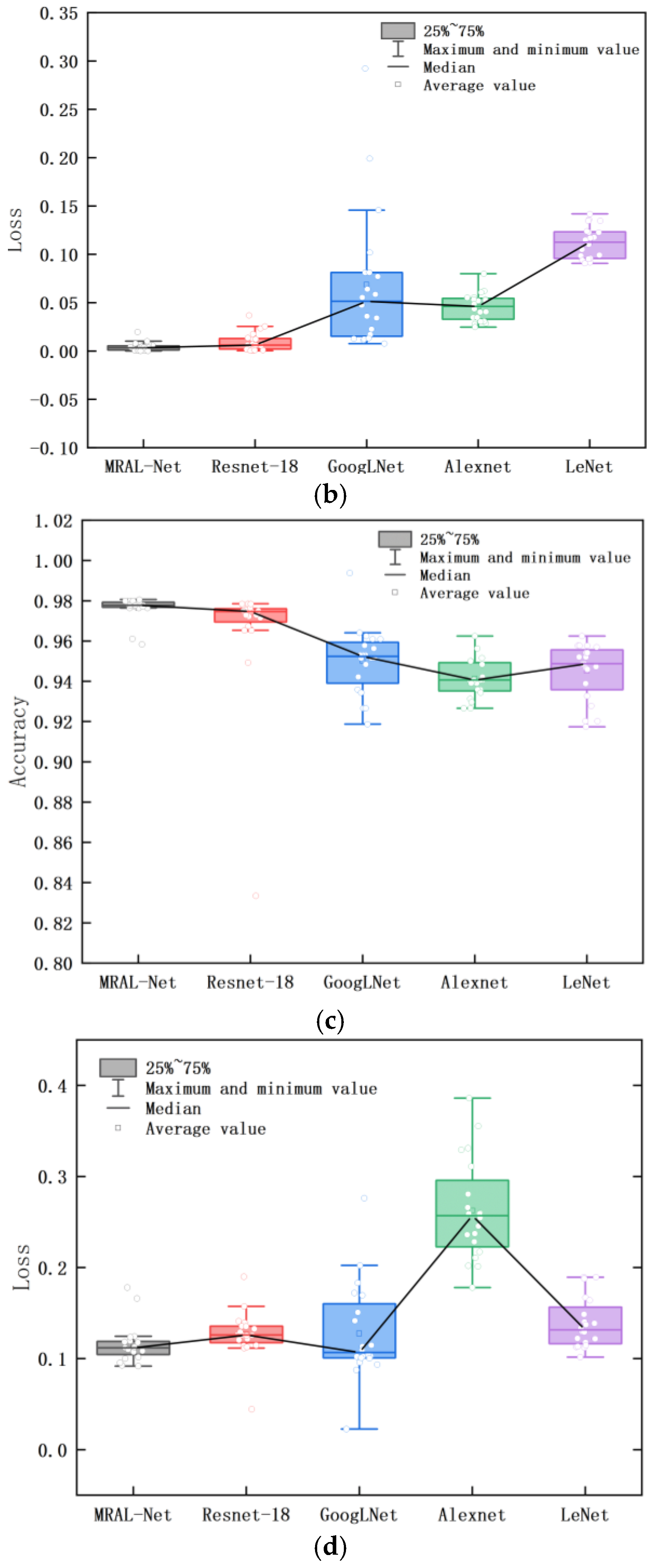
Figure 20.
The average accuracy of the five network models corresponding to the four states.
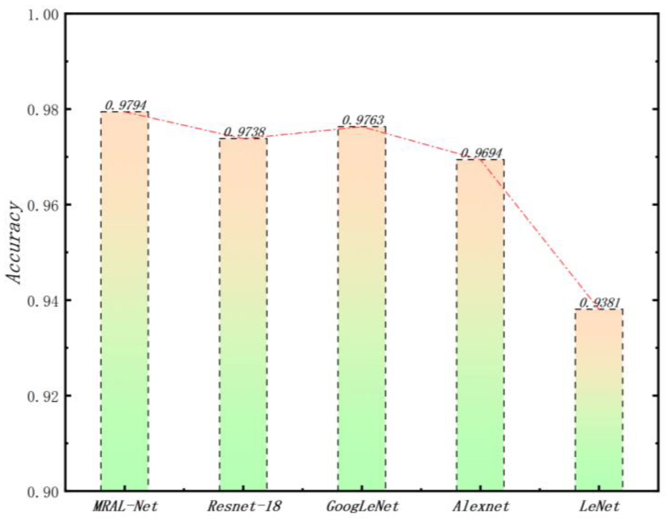
Figure 21.
Ablation test results.
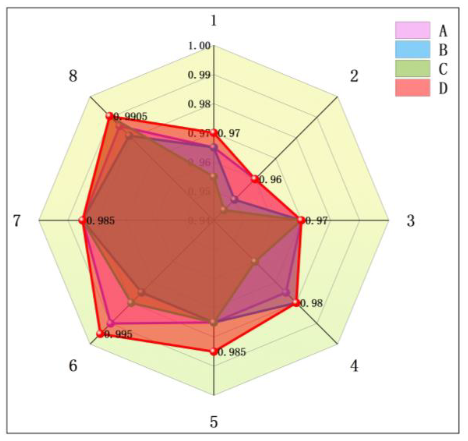
Figure 22.
Comparison of the accuracy of the five networks combined with time-frequency analysis methods.
Figure 22.
Comparison of the accuracy of the five networks combined with time-frequency analysis methods.
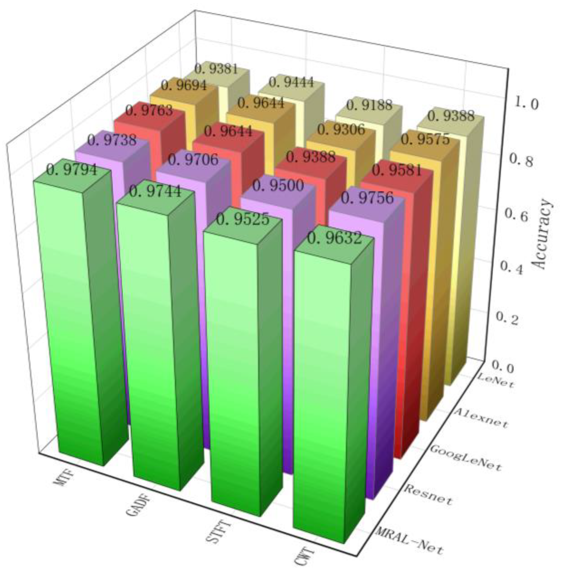

Table 1.
Parameters of each network layer.
| Kernel Size | Strides | Padding | Repeat | Output | Output Channels | |
|---|---|---|---|---|---|---|
| Conv | 7×7 | 2 | 3 | 112×112 | 64 | |
| CBAM | 1×1/7×7 | 112×112 | 64 | |||
| Maxpool | 3×3 | 2 | 1 | 56×56 | 64 | |
| Residual1 | 3×3 | 1 | 1 | 2 | 56×56 | 64 |
| Residual2 | 3×3 | 2 | 1 | 28×28 | 128 | |
| Residual3 | 3×3 | 1 | 1 | 28×28 | 128 | |
| Residual4 | 3×3 | 2 | 1 | 14×14 | 256 | |
| Residual5 | 3×3 | 1 | 1 | 14×14 | 256 | |
| Residual6 | 3×3 | 2 | 1 | 7×7 | 512 | |
| Residual7 | 3×3 | 1 | 1 | 7×7 | 512 | |
| AvgPool | 1×1 | 512 | ||||
| Flatten | 1 | 512 | ||||
| LSTM1 | 128 | |||||
| LSTM2 | 128 | |||||
| Linear | 4 |
Table 2.
Number of samples in the training and test sets.
| Training Sample | Validation Sample | Testing Sample | Total Sample | |
|---|---|---|---|---|
| Normal | 1440 | 360 | 400 | 2200 |
| Iron core loosening | 1440 | 360 | 400 | 2200 |
| Winding loosening | 1440 | 360 | 400 | 2200 |
| Iron core and winding loose | 1440 | 360 | 400 | 2200 |
Table 3.
SE, VCR, and CC values of each IMF component.
| IMF1 | IMF2 | IMF3 | IMF4 | IMF5 | IMF6 | IMF7 | IMF8 | IMF9 | IMF10 | |
|---|---|---|---|---|---|---|---|---|---|---|
| SE | 1.9798 | 1.6196 | 0.6316 | 0.6289 | 0.2782 | 0.0678 | 0.0953 | 0.0538 | 0.0254 | 0.0092 |
| VCR | 0.0461 | 0.0124 | 0.3065 | 0.0380 | 0.5652 | 0.0263 | 0.0043 | 0.0008 | 0.0002 | 0.0003 |
| CC | 0.0024 | 0.0161 | 0.5860 | 0.3916 | 0.7481 | 0.1521 | 0.0120 | 0.0037 | 0.0031 | 0.0039 |
Table 4.
Accuracy and loss rate of each model after stabilization.
| Model | The Average Accuracy of the Training Set | The Average Accuracy of the Validation Set | The Training Set Average Loss Rate | Validation Set Average Loss Rate |
|---|---|---|---|---|
| MRAL-Net | 0.9986 | 0.9764 | 0.0041 | 0.1157 |
| Resnet-18 | 0.9970 | 0.9655 | 0.0093 | 0.1264 |
| GoogLeNet | 0.9759 | 0.9501 | 0.0685 | 0.1272 |
| Alexnet | 0.9822 | 0.9411 | 0.0455 | 0.2624 |
| LeNet | 0.9559 | 0.9449 | 0.1121 | 0.1385 |
Table 5.
Time spent on training each model.
| Model | MRAL-Net | Resnet-18 | GoogLeNet | Alexnet | LeNet |
|---|---|---|---|---|---|
| Times | 1705s | 1892s | 2146s | 1538s | 1355s |
Table 6.
Confusion matrix and precision, recall, and F1 score of the proposed method.
| MRAL-Net | Prediction Label | Precision | Recall | F1-Score | ||||
|---|---|---|---|---|---|---|---|---|
| 0 | 1 | 2 | 3 | |||||
| True label | 0 | 400 | 0 | 0 | 0 | 1 | 1 | 1 |
| 1 | 0 | 386 | 0 | 14 | 0.9674 | 0.9650 | 0.9662 | |
| 2 | 0 | 0 | 400 | 0 | 0.9852 | 1 | 0.9925 | |
| 3 | 0 | 13 | 6 | 381 | 0.9646 | 0.9525 | 0.9585 | |
| Accuracy | 97.9375% | — | ||||||
Table 7.
Performance of the five network models corresponding to the four states.
| Precision | Recall | F1 score | |
|---|---|---|---|
| MRAL-Net | 0.9830 | 0.9794 | 0.9812 |
| Resnet-18 | 0.9754 | 0.9744 | 0.9749 |
| GoogLeNet | 0.9763 | 0.9756 | 0.9759 |
| Alexnet | 0.9699 | 0.9694 | 0.9696 |
| LeNet | 0.9424 | 0.9381 | 0.9402 |
Disclaimer/Publisher’s Note: The statements, opinions and data contained in all publications are solely those of the individual author(s) and contributor(s) and not of MDPI and/or the editor(s). MDPI and/or the editor(s) disclaim responsibility for any injury to people or property resulting from any ideas, methods, instructions or products referred to in the content. |
© 2025 by the authors. Licensee MDPI, Basel, Switzerland. This article is an open access article distributed under the terms and conditions of the Creative Commons Attribution (CC BY) license (http://creativecommons.org/licenses/by/4.0/).
Copyright: This open access article is published under a Creative Commons CC BY 4.0 license, which permit the free download, distribution, and reuse, provided that the author and preprint are cited in any reuse.


