
Submitted:
29 November 2025
Posted:
02 December 2025
You are already at the latest version
Abstract
This work proposes a mechanism initiating the Big Bang: the Universe emerged from the collapse of the densest object in a previous-aeon black hole. While the object collapsed into the Big Bang singularity with minimum entropy, the entropy of the host black hole kept increasing. The Second Law of thermodynamics was never violated. The collapse was the reverse of cosmic inflation. Where it occurred, or the Center of the Universe, is found to be currently ~30 billion light years away from us and around Galactic coordinates (l,b)=(279°,-47°). If a Universal Coordinate System is defined accordingly, we are in the Northern Universe at the latitude: W=+35°. Since last scattering, the nearly isotropic and homogeneous Universe is found to have spun clockwise through an angle of 41°±6°, whereas it is calculated to be 49°+7°-11° by a modified Friedmann equation using the early- and late-Universe Hubble constants. The findings are supported by other independent observations.
Keywords:
cosmology
; cosmic background radiation — early Universe
Introduction
To support Penrose’s conformal cyclic cosmology (CCC) [1,2], Gurzadyan and Penrose presented a map of temperature low-variance circles (LVCs) based on the cosmic microwave background (CMB) data [2,3,4]. From the WMAP data, they found a large, higher-temperature LVC region X concentrated around , and a small, lower-temperature region Y around [3]. When updating their search on the Planck data, they found two other large LVC regions. Since they did not name them, we assign names accordingly (Figure 1): the lower-temperature region Z concentrated at , and temperature-dipole region W at [2,4].
The LVCs have been interpreted to arise from previous-aeon supermassive black-hole encounters [2,3,4], but CCC does not predict the location of the LVCs. In this work, we postulate a mechanism initiating the Big Bang, with which the anisotropic distribution of the LVC regions and many other astronomical observations can be explained.
Postulated Mechanism
In CCC, the crossover between aeons is future null infinity [1,2]. This work, instead, assumes that the crossover is the collapse of the densest object (DO), an idea similar to those suspected by former researchers, such as King [5], Smolin [6], and Penrose [1]. The DO was incubated in the previous aeon: all the falling mass-energy was in a process of being immobilized as the densest matter, making the DO grow continually. Once its mass exceeded a limit, the DO collapsed. Because it had already been the most dense, the only possible product of the collapse was an infinitesimal pure energy point, i.e. the Big Bang singularity, from which this Universe was created. The DO or Big Bang singularity is the Center of the Universe.
The densest objects that can be directly observed are neutron stars. For a spinning neutron star, there is an equatorial plane, perpendicular to its axis of spin. Objects fall towards the spinning star in spirals. The star emits twin emission beams symmetric about the star. If the beams misalign the axis of spin, then it is a pulsar [7]. We further assume that the surroundings of the DO were analogous to those of a pulsar (Figure 2).
After the collapse, the isotropic Big Bang expansion wave VU from the Center collided with the highly anisotropic surroundings of the DO. Because the emission beams Vb of the DO had the same direction (away from the Center) as VU, less collisions occurred, leading to twin lower-temperature trajectories symmetric about the Center. If the Center is within our observable universe, the trajectories intersecting with the surface of last scattering (SLS) resulted in a pair of cold spots in the CMB sky. Simultaneously, since the falling spiral flows Vs of the DO had obtuse angles with VU, their collisions led to higher-temperature spirals. The spirals intersecting with the SLS generated hot regions.
All the collisions, including those between Vb and VU, resulted in overdense clumps in the primordial plasma. These clumps, comprised of dark matter, photons, and baryonic particles, as local centers, produced outward pressure. The outward pressure and inward gravity created oscillations or spherical waves. By enhancing local mass and heat transfer, the oscillations, like smoothers, lowered temperature variance, leaving behind LVCs. Therefore, the LVCs arose completely in this aeon (different from CCC); this generation process was similar to baryon acoustic oscillations (BAO). As it was a dynamic process, the window to observe the LVC regions would be narrow: if formed too early, then LVCs would have dissipated; if too late, then LVCs would not have formed by the time of last scattering.
The Center and spin of the Universe
Since the collision signals from the baby Universe have become vague: large in scale, small and noisy in intensity, in this work we focus on large-scale signals. As region Z is the only large region with predominantly lower temperatures (Figure 3c), Vb cannot be determined solely by the LVC signals. We therefore check the cold spots with maximum temperature depressions. Bennett et al. [8] were the first to find two cold spots in the CMB: Cold Spot I and Cold Spot II. By studying large-scale extrema, the Planck Collaboration [9,10] confirmed both spots: (the maximum depression at ) at Peak 1 and at Peak 5 (another minimum, Peak 2, is not a typical cold spot, with merely -25 µK depression at , but with larger depressions off-center: , Figure 30 in [9]). We label the cold spot at as the north cold spot (NC), corresponding to Cold Spot I and Peak 1, and the one at as the south cold spot (SC), corresponding to Cold Spot II and Peak 5.
To evaluate the symmetry of the cold spots about the Center, we define a synchronous ratio: , where R is the distance to the Center. If the cold spots are distributed at equal distances about the Center (), by linking NC and SC with a line (line NC-SC), its intersection with the Vs plane is the Center.
Region X has higher temperatures, and region W (more obvious in Figure 31 in Penrose’s Nobel Lecture [2]) is a temperature dipole: one end is hotter and the other colder (Figure 1and Figure 3). Both regions correspond to Vs. For region X, although part of it is within the excluded galactic disk , it is obvious that the center is at its central void: [2,4]. The center of region W: is obtained by taking an average of the xyz-coordinates of its LVC points from figures in [2,4].
Line XW almost intersects line NC-SC (the shortest distance between the lines is only 0.07). Therefore, the closest point on line NC-SC, at and a distance away, can be approximated to be the Center, where is the radius of the SLS: at last scattering, ; at present, [11]. More accurately, the Vs plane can be determined by adding a region with maximum temperature elevation: the Planck Collaboration’s Peak 3 ( [9]) concentrated at (from figures in [10]). The obtained Vs plane is:
Therefore, the intersection (Figure 4) of line NC-SC and the Vs plane, or the Center, is at and at a distance (currently 9.3 Gpc or 30 billion light years) away.
It is vital to note that region X has a small cold part near (Figure 3b), facing the cold end of region W (Figure 1 and Figure 3d). These lower-temperature signals, versus the higher-temperature signals on the opposite section of the Vs disk, indicate that the DO, and consequently the Universe, must spin (see Evidence III for detailed analysis). If we look from where we are, i.e. the Local Supercluster (LS), to the Center, the Universe spins clockwise. The axis of spin is:
The coordinates of the Center and the direction of spin obtained in this work are virtually the same as those purely from the temperature anisotropy of the CMB [12].
Support for the Postulated Mechanism
Considering that the Universe has long been believed to have no center, we provide 11 pieces of evidence to support our mechanism. For convenience, we define a Universal Coordinate System (UCS): the Center is chosen as the origin, the Vs plane as the Universal equatorial plane, the LS at zero degrees longitude, the direction of spin as the direction of longitude increase, and the comoving radius of the SLS as the unit length. For example, the angle between the equatorial plane and the line through the LS and the Center is ca. , so our UCS longitude, latitude, and radius are: (Figure 5).
Evidence I. Observation. It is remarkable to note that region Z, concentrated at , has the same UCS latitude as does NC at , and that the main body of region Z has lower-temperature LVCs (Figure 3c). Our mechanism thus has a crucial piece of evidence: region Z was generated by the northern Vb.
Evidence II. Method. After the DO collapse, the Big Bang expansion wave VU collided with the surrounding beams Vb and flows Vs. While they were pushed away from the Center, all of the beams and flows were swallowed by VU (eventually, the collision clumps were expanding with the Universe: , and ). The motions of the collision clumps relative to VU along the radial directions can be called Universal peculiar radial motions. Based on the method used in this work, the peculiar radial motions do not affect the determination of line NC-SC and the Vs plane.
Because of the existence of region Z, it is known that the Vb beams were emitted in straight lines along the radial directions, much further than NC at , and the closer SC at . The synchronous ratio: indicates that the cold spots were located roughly symmetrically about the Center (Figure 4). However, because it is not absolutely symmetric: , it is required to consider another important factor, the angular speed of the DO spin. As shown in the Mollweide projection (Figure 4.1 in [10]), the cold spots (Peaks 1 and 5) are ellipses, indicating that, compared to the emission speed of the Vb beams, the DO spun at a much smaller speed (Figure 6 and Appendix A). This property ensures that the small asymmetry: is insignificant for the calculation of the coordinates of the Center.
The larger temperature depression of SC than NC [9] also indicates that the obtained Center is reasonable, though the depression is often interpreted using the Integrated Sachs-Wolfe effect [13]. As it was closer to the Center, the Vb beam at SC had a higher mass-energy density (the outgoing Vb was scattered by the falling drops of Vb: ) and a higher outgoing speed, and consequently a larger depression: .
Evidence III. Method. Since the early last century, physicists have carefully studied Mach’s principle, or more specifically, Mach’s postulate of relativity of rotation [14]. Using Einstein’s shell-type model, Brill and Cohen first discovered that there exists “perfect dragging” in the interior of a slowly rotating mass shell with the Schwarzschild radius [15]. This fundamental conclusion is confirmed by many others e.g. [16,17,18,19,20,21]. Our slowly spinning Universe (Appendix C) is within its host black hole (Appendices F and I). The perfect dragging ensures all the objects of the Universe spin with the Universe: . From our (in the interior of the Universe) perspective, the spacetime of the Universe does not spin or rotate (Appendix B):
Note that there is no speed limit to the rotation or expansion of spacetime itself. Both superluminal expansion velocity and superluminal rotation (from the exterior perspective) are allowed by the general theory of relativity [19].
When they collided with VU, the spiral flows Vs plunged into the expanding Universe that was spinning with decreasing angular speed: . The collisions between Vs and VU elevated the temperatures in the Vs area. Note that the temperature elevation is highly dependent on the distance to the Center: . Considering that for the temperature depression by the Vb that collided with VU in the same direction, we know that for the temperature elevation by the Vs that collided with VU in the opposite directions (both were strongly dependent on the distance R). At distances close to the Center, such as region X and Peak 3, the collisions were the strongest and the temperatures were the highest (more discussion in Appendix A).
Based on our mechanism, right before the Big Bang, the spiral flows Vs from the exterior had fell into the host black hole for the growth of the DO. The high-velocity (versus that of the circulating flows, Figure 2) spiral flows Vs can be observed in the CMB, due to their extra rotations relative to the spin of the Universe: (eventually, the angular speed of the collision clumps asymptote to that of the Universe: ). The extra rotations can be called Universal peculiar rotations (about the axis of spin of the Universe). The peculiar rotations of regions X and W, and Peak 3 do not affect the determination of the Vs plane.
Region X, concentrated at , is located behind the axis of spin. On the side where the collision clumps of region X peculiarly rotated towards us, the Doppler effect elevated the temperatures. On the other side where they peculiarly rotated away from us, the Doppler effect and collision effect cancelled each other, hence the temperatures are averaged out or slightly lower. As we expected, the higher-temperature part (Figure 3a) and the relatively-lower-temperature part (Figure 3b) of region X are clearly divided by the plane: , indicating that the peculiar rotations of region X are clockwise. Because of the frame dragging, and had the same direction; the Universe spun clockwise. The alignment of the observer, the axis of spin, and the dividing plane of region X directly proves our mechanism. The peculiar rotations are also observed in region W, and will be discussed in Evidence VII.
Evidence IV. Nearly isotropic and homogeneous Universe. After the collapse of the DO, the Big Bang first created a rebounded counterpart of the DO (Appendices I and J). Guth, Linde, and others established inflation theory for the very early Universe [22,23,24,25,26]. Primordial inflation [23,24] was proposed starting at the Planck time in the context of the Theory of Everything (TOE): . Combined with the inflation from to sec in the context of the Grand Unified Theory (GUT) [22,23,24,25,26]: to make double inflation [24,25], we have the beauty of symmetry:
The expansion velocity for any object in the Universe was proportional to its proper distance to the Center: , where the Hubble parameter can be calculated using the first Friedmann equation. This velocity profile dominates the entire course of the expansion. Therefore, even though we in the LS are flying away from the Center, we can observe the recession velocity:
where is the proper distance to us. Light travels in the spacetime of the Universe (Appendix B), so if objects are too far away and , then we will never see them. Together with the perfect frame dragging (equation 3), equation (5) ensures that the CMB temperature (after removing the CMB dipole) is uniform. With this velocity profile, the Universe is isotropic and homogeneous.
Without enough gravitational force (after the Big Bang, the Center had no massive DO left), the rotational energy of the Universe was inevitably converted into the extra energy of expansion in the two-dimensional rotation plane parallel to the equator, not in the direction parallel to the axis of spin; hence the Universe veered into ellipsoidal (see Figure 5; note that Pfister and Braun first found that a rotating universe with flat geometry is not exactly spherical [27]).
However, the deformation did not necessarily make the Universe significantly anisotropic or inhomogeneous. This is because most of the rotational energy had been converted into that of expansion before the Universe was 100 Myr old (see Evidence V). Since the original increase of velocity was always accompanied with the increase of distance, this energy was eventually dissipated into potential energy (i.e., the first term on the right side of equation C.4). As the Universe further expanded, significant extra energy was no longer available. The ratio of recession velocity versus distance: depends on the energy densities as the Friedmann equation predicts.
Evidence V. Hubble tension. At last scattering, the Universe had invisible rotational energy. At present, almost all the rotational energy has been converted into that of expansion. Therefore, the spinning early Universe had a smaller observable Hubble constant; the non-spinning late Universe has a larger observable Hubble constant. This mismatch of the Hubble constants is known as the Hubble tension.
Because the spinning Universe is nearly isotropic and homogeneous, the Friedmann equation is modified for a quick analysis (see Appendix C; note that Klein first embedded a slowly rotating mass shell with flat interior in a Friedmann universe [18]). By comparing Riess et al.’s latest reported late-Universe constant [28]: with the constant at last scattering [29]: , we obtain the angular speed at last scattering (equation C.12): , and that at present: (slow enough to be regarded as non-spinning).
Using equation (C.13), the observable Hubble constant is calculated for different scale factors a of the Universe after last scattering. After the Universe was 100 Myr old (), becomes very stable (Figure 7). For example, the JWST can observe objects with redshifts up to ; the calculated constant: . The difference: is much smaller than the uncertainty of measurement [28]. Indeed, what the JWST observed [28,30] is the late-Universe .
Evidence VI. Spatial anisotropies. Although appears stable if , there was a small portion of the rotational energy remaining, part of which was converted into that of anisotropic expansion. Obviously, if the isotropic Hubble expansion is removed, the slowest expansion direction (SED) points towards the axis of spin (Figure 5). Many researchers have observed that the Universe does have very small anisotropies e.g. [31,32,33,34,35,36,37,38,39,40,41]. As predicted, the observed anisotropic directions do point towards the axis of spin (Appendix G, Table 1, and Figure 8). The observed magnitudes of anisotropies, in the range of 10-5 to 10-3, are also reasonable. For example, for the dark energy dipole [32] observed with redshifts: , the remaining rotational energy was: (equation C.11).
Campanelli et al. believed that the SLS was ellipsoidal (the eccentricity from the CMB anisotropy: ) [35]. Based on our mechanism, the observable universe is not exactly ellipsoidal, because it does not have orthogonal axes as the Universe does or, equivalently, we are not on the Universal equatorial plane (Figure 5). Considering that the observed anisotropies are small, the SLS approximates to a sphere for the calculation of the coordinates of the Center in this work.
Evidence VII. Angle of spin. Region W, concentrated at , is far away from the Center, with very small temperature elevations from the collisions between Vs and VU. On the other hand, while the Universe spun more slowly as it expanded far away from the Center, the peculiar rotations of the spiral flows Vs became more obvious. The Doppler effect tells us that the characteristic dipole pattern (Figure 3d) can only be observed if the observer was in the middle of region W at last scattering: (Figure 9). If the speed of light were infinity, it could be seen anywhere on the plane: . On the other hand, even if the speed of light were infinity, what we in the LS at present can observe would only be the dipole on the plane: . But we happen to observe it now! Since the speed of light is limited, this characteristic dipole signal took 13.8 billion years to arrive at us. During this period, the Universe has spun through an angle of so that the two planes: and overlap.
We use the modified first Friedmann equation to calculate the angle that the Universe has spun through: (Appendix D). Considering the independence of these two pathways, we conclude that the angles of spin have a good match.
Evidence VIII. Observation. All the other details of Gurzadyan and Penrose’s LVC map [2,3,4] and the Planck Collaboration’s large-scale extrema [9,10] are interpreted by our mechanism (Appendix A).
Evidence IX. Comparison to CCC. As we know, black holes have maximum entropy (e.g. for a black hole with mass , its entropy: , where kB is the Boltzmann constant), while the Big Bang singularity has minimum entropy (). It seems obvious that an evolution from a black hole to the Big Bang singularity immensely violates the Second Law of thermodynamics. Penrose therefore chose the ultimate hypersurface to be the crossover in CCC [1,2].
In our mechanism, the precursor DO, excluding all the flows, did collapse into the Big Bang singularity with minimum entropy. However, the DO was absolutely not an isolated system, because the mass-energy flows were continuously falling into and emitting from it (Appendix E and Figure 2). On the other hand, the collapse and the resulting Big Bang occurred completely within the host black hole. From the exterior (i.e. the previous aeon, Figure 10) perspective, it was a normal black hole; its entropy kept increasing as the mass increased: . Therefore, even if the host black hole is considered as an isolated system, the Second Law is still sustained.
Evidence X. Unexpected structures. The unexpected first galaxies [42,43,44,45] observed by the JWST (Appendix H) would originate from overdense collision clumps as primordial nucleation centers (PNCs), thus they grew much faster than predicted by structure formation theories. PNCs would also directly become primordial black holes [46,47,48].
Evidence XI. DO and the counterpart. Kerr believes that ellipsoidal ultra-dense bodies, instead of ring singularities, would exist within spinning black holes [49]. The DO and the counterpart were such bodies. While they were curvature singularities (Appendix I), the DO eventually collapsed into the Big Bang singularity (Penrose singularity theorem), and then the singularity created the counterpart (Hawking singularity theorem). By further providing what the DO and the counterpart would be (Appendix J), our mechanism is more convincing.
Conclusions
The Universe emerged from the collapse of the densest object in a previous-aeon black hole. Nature exists before the Big Bang (in time) and outside this Universe (in space) (Figure 10).
Acknowledgments
J.B.B. would like to thank Profs. Z. Shen, K. Yao, X. Jiang, F. Bo, Y. Cheng, S. Han, G. Chen, and Q. Yu at Zhejiang University for their inspiration. N.P.B. would like to dedicate this work to his grandparents in China.
References
- R. Penrose, Cycles of time: an extraordinary new view of the universe (Bodley Head, London, 2010).
- R. Penrose, Black holes, cosmology and space-time singularities. Nobel Lecture, Dec. 8, 2020. https://www.nobelprize.org/uploads/2024/02/penrose-lecture.pdf.
- V. G. Gurzadyan, and R. Penrose, On CCC-predicted concentric low-variance circles in the CMB sky. Eur. Phys. J. Plus. 128, 22 (2013). [CrossRef]
- V. G. Gurzadyan, and R. Penrose, CCC and the Fermi paradox. Eur. Phys. J. Plus. 131, 11 (2016). [CrossRef]
- A. R. King, New types of singularity in general relativity: the general cylindrically symmetric stationary dust solution. Commun. Math. Phys. 38, 157-171 (1974). [CrossRef]
- L. Smolin, The life of the Cosmos (Oxford Univ. Press, New York, 1997).
- The Rapid Burster. https://images.nasa.gov/details-PIA21418.
- C. L. Bennett et al., Seven-year Wilkinson Microwave Anisotropy Probe (WMAP) observations: are there cosmic microwave background anomalies? Astrophys. J. Supp. Ser. 192, 17 (2001). [CrossRef]
- Planck Collaboration: Y. Akrami et al., Planck 2018 results. VII. Isotropy and statistics of the CMB. Astron. Astrophys. 641, A7 (2020). [CrossRef]
- A. Marcos-Caballero, The Cosmic Microwave Background radiation at large scales and the peak theory (Univ. Cantabria Thesis, 2017).
- J. R. Gott III et al., A map of the universe. Astrophys. J. 624, 463-484 (2005). [CrossRef]
- J.-B. Bao, and N. P. Bao, On the fundamental particles and reactions of nature. Preprint, 2020120703 (2021). [CrossRef]
- A. Kovács et al., The DES view of the Eridanus supervoid and the CMB Cold Spot. Mon. Not. R. Astron. Soc. 510, 216-229 (2021). [CrossRef]
- E. Mach, Die Geschichte und die Wurzel des Satzes von der Erhaltung der Arbeit. (Calve, Prag, 1872).
- D. R. Brill, and J. M. Cohen, Rotating masses and their effect on inertial frames. Phys. Rev. 143, 1011-1015 (1966). [CrossRef]
- V. De La Cruz, and W. Israel, Spinning shell as a source of the Kerr metric. Phys. Rev. 170, 1187-1192 (1968). [CrossRef]
- H. Pfister, and K. H. Braun, A mass shell with flat interior cannot rotate rigidly. Class. Quantum Grav. 3, 335-345 (1986). [CrossRef]
- C. Klein, Rotational perturbations and frame dragging in a Friedmann universe. Class. Quantum Grav. 10, 1619-1631 (1993). [CrossRef]
- O. G. Gron, The principle of relativity and inertial dragging. Am. J. Phys. 77, 373-380 (2009). [CrossRef]
- C. Schmid, Mach’s principle: Exact frame-dragging via gravitomagnetism in perturbed Friedmann-Robertson-Walker universes with K = (±1, 0). Phys. Rev. D 79, 064007 (2009). [CrossRef]
- S. Braeck, Inertial frame dragging and relative rotation of ZAMOs in axistationary asymptotically flat spacetimes. Universe 9, 120 (2023). [CrossRef]
- A. H. Guth, Inflationary universe: a possible solution to the horizon and flatness problems. Phys. Rev. D 23, 347-356 (1981). [CrossRef]
- J. Ellis et al., Primordial supersymmetric inflation. Nucl. Phys. B 221, 524-548 (1983). [CrossRef]
- A. D. Linde, The inflationary universe. Rep. Prog. Phys. 47, 925-986 (1984). [CrossRef]
- J. Silk, and M. S. Turner, Double inflation. Phys. Rev. D 35, 419-428 (1987). [CrossRef]
- A. H. Guth, Lecture 23: inflation (MIT Open Course Ware, 2013).
- H. Pfister, and K. H. Braun, Induction of correct centrifugal force in a rotating mass shell. Class. Quantum Grav. 2, 909-918 (1985). [CrossRef]
- A. G. Riess et al., JWST validates HST distance measurements: Selection of supernova subsample explains differences in JWST estimates of local H0. Astrophys. J. 977, 120 (2024). [CrossRef]
- Planck Collaboration: N. Aghanim et al., Planck 2018 results. VI. Cosmological parameters. Astro. Astrophys. 641, A6 (2020). [CrossRef]
- A. G. Riess et al., JWST observations reject unrecognized crowding of Cepheid photometry as an explanation for the Hubble tension at 8σ confidence. Astrophys. J. Lett. 962, L17 (2024). [CrossRef]
- J. A. King et al., Spatial variation in the fine-structure constant – new results from VLT/UVES. Mon. Not. R. Astron. Soc. 422, 3370-3414 (2012). [CrossRef]
- A. Mariano, and L. Perivolaropoulos, Is there correlation between fine structure and dark energy cosmic dipoles? Phys. Rev. D 86, 083517 (2012). [CrossRef]
- Z. Chang, and H.-N. Lin, Comparison between hemisphere comparison method and dipole-fitting method in tracing the anisotropic expansion of the Universe use the Union2 data set. Mon. Not. R. Astron. Soc. 446, 2952–2958 (2015). [CrossRef]
- K. Migkas et al., Cosmological implications of the anisotropy of ten galaxy cluster scaling relations. Astro. Astrophys. 649, A151 (2021). [CrossRef]
- L. Campanelli, P. Cea, and L. Tedesco, Ellipsoidal universe can solve the CMB quadrupole problem. Phys. Rev. Lett. 97, 131302 (2006). [CrossRef]
- A. Kashlinsky et al., A measurement of large-scale peculiar velocities of clusters of galaxies: technical details. Astrophys. J. 691, 1479–1493 (2009). [CrossRef]
- H. A. Feldman, R. Watkins, and M. J. Hudson, Cosmic flows on 100 h−1 Mpc scales: standardized minimum variance bulk flow, shear and octupole moments. Mon. Not. R. Astron. Soc. 407, 2328–2338 (2010). [CrossRef]
- S. J. Turnbull et al., Cosmic flows in the nearby universe from Type Ia supernovae. Mon. Not. R. Astron. Soc. 420, 447–454 (2012). [CrossRef]
- E. Abdalla et al., Cosmology intertwined: A review of the particle physics, astrophysics, and cosmology associated with the cosmological tensions and anomalies. J. High Energy Astrophys. 34, 49-211 (2022). [CrossRef]
- L. Perivolaropoulos, and F. Skara. Challenges for ΛCDM: An update. New Astron. Rev. 95, 101659 (2022). [CrossRef]
- P. K. Aluri et al., Is the Observable Universe Consistent with the Cosmological Principle? Class. Quantum Grav. 40, 094001 (2023). [CrossRef]
- A. Witze, Four revelations from the Webb telescope about distant galaxies. Nature 608, 18-19 (2022). [CrossRef]
- D. Clery, Earliest galaxies found by JWST confound theory. Science 379, 1280-1281 (2023). [CrossRef]
- I. Labbé et al., A population of red candidate massive galaxies ~600 Myr after the Big Bang. Nature 616, 266-269 (2023). [CrossRef]
- M. Boylan-Kolchin, Stress testing ΛCDM with high-redshift galaxy candidates. Nat. Astron. 7, 731-735 (2023). [CrossRef]
- J. Silk et al., Which came first: supermassive black holes or galaxies? Insights from JWST. Astrophys. J. Lett. 961, L39 (2024). [CrossRef]
- A. Matteri, A. Ferrara, and A. Pallottini, Beyond the first galaxies primordial black holes shine. Astro. Astrophys. 701, A186 (2025). [CrossRef]
- P. G. Perez-Gonzalez et al., The rise of the galactic empire: ultraviolet luminosity functions at z ~ 17 and z ~ 25 estimated with the MIDIS+NGDEEP ultra-deep JWST/NIRCam dataset. Astrophys. J. 991, 179 (2025). [CrossRef]
- R. P. Kerr, Do black holes have singularities? ArXiv:2312.00841 (2023). [CrossRef]
- de Oliveira-Costa, A. et al. Significance of the largest scale CMB fluctuations in WMAP. Phys. Rev. D 69, 063516 (2004). [CrossRef]
- A. Wright, Across the universe. Nat. Phys. 9, 264 (2013). [CrossRef]
- D. R. Faulkner, The Axis of Evil and the cold spot—serious problems for the Big Bang? Answer Depth, 13 (2018). https://answersingenesis.org/big-bang/axis-evil-cold-spot-sea-rious-problems-big-bang/.
- E. Bodnia et al., The quest for CMB signatures of conformal cyclic cosmology. J. Cosmol. Astropart. Phys. 2024 (05), 009 (2024). [CrossRef]
- Planck Collaboration: P. A. R. Ade et al., Planck 2015 results. XVI. Isotropy and statistics of the CMB. Astron. Astrophys. 594, A16 (2016). [CrossRef]
- B. Ryden, Introduction to Cosmology. 2nd. edn. (Cambridge Univ. Press, Cambridge, 2017).
- D. Castelvecchi, Is dark energy getting weaker? Fresh data bolster shock finding. Nature, 639, 849 (2025). [CrossRef]
- P. C. W. Davies, T. M. Davis, and C. H. Lineweaver, Black holes constrain varying constants. Nature 418, 602-603 (2003). [CrossRef]
- S. Carlip, and S. Vaidya, Do black holes constrain varying constants? Nature 421, 498 (2003). [CrossRef]
- A. Kogut et al., Dipole anisotropy in the Cobe differential microwave radiometers first-year sky maps. Astrophys. J. 419, 1-6 (1993). [CrossRef]
- M. Aaronson et al., A distance scale from the infrared magnitude/H I velocity-width relation. V. Distance moduli to 10 galaxy clusters, and positive detection of bulk supercluster motion toward the microwave anisotropy. Astrophys. J. 302, 536-563 (1986). [CrossRef]
- The Virgo Cluster of Galaxies. http://www.messier.seds.org/more/virgo.html.
- D. Lynden-Bell et al., Photometry and Spectroscopy of Elliptical Galaxies. V. Galaxy Streaming toward the New Supergalactic Center. Astrophys. J. 326, 19-49 (1988). [CrossRef]
- Voyage to the Great Attractor. https://lweb.cfa.harvard.edu/~dfabricant/huchra/seminar/attractor/.
- M. Ahlers, Deciphering the dipole anisotropy of galactic cosmic rays. Phys. Rev. Lett. 117, 151103 (2016). [CrossRef]
- The Pierre Auger Collaboration: A. Aab et al., Observation of a large-scale anisotropy in the arrival directions of cosmic rays above 8 × 10¹⁸ eV. Science 357, 1266-1270 (2017). [CrossRef]
- R. B. Tully, C. Howlett, and D. Pomarède, Ho’oleilana: An individual baryon acoustic oscillation? Astrophys. J. 954, 169 (2023). [CrossRef]
- List of most massive black holes. https://www.wikipedia.org/wiki/List_of_most_massive_black_holes.
- V. A. Belinskii, I. M. Khalatnikov, and E. M. Lifshitz, Oscillatory approach to a singular point in the relativistic cosmology. Adv. Phys. 19, 525-573 (1970). [CrossRef]
- M. A. Scheel, and K. S. Thorne, Geometrodynamics: the nonlinear dynamics of curved spacetime. Physics-Uspekhi 57, 342-351 (2014). [CrossRef]
- R. Penrose, Singularities and Time-Asymmetry. In S. W. Hawking, and W. Israel, General Relativity: An Einstein Centenary Survey (Cambridge University Press, Cambridge, 581-638, 1979).
- Ya. B. Zel’dovich, Creation of particles in cosmology. In M. S. Longair, Confrontation of cosmological theories with observational data (D. Reidel Pub., Dordrecht, 329-333, 1974).
- P. Ramond, Gauge theories and their unification. Ann. Rev. Nucl. Part. Sci. 33, 31-66 (1983). [CrossRef]
- D. Perkins, Particle Astrophysics. 2nd edn. (Oxford Univ. Press, New York, 2003).
- N. Prakash, Dark matter, neutrinos, and our solar system (World Sci., Singapore, 2013).
- J. A. Formaggio, and G. P. Zeller, From eV to EeV: neutrino cross sections across energy scales. Rev. Mod. Phys. 84, 1307-1341 (2012). [CrossRef]
- IceCube Collab., Measurement of the multi-TeV neutrino interaction cross-section with IceCube using Earth absorption. Nature, 551, 596-600 (2017). [CrossRef]
- R. Barbieri et al., Baryogenesis through leptogenesis. Nucl. Phys. B 575, 61-77 (2000). [CrossRef]
- A. Abada et al., Flavour matters in leptogenesis. J. High Eng. Phys. 09, 010 (2006). [CrossRef]
Figure 1.
A schematic diagram of the LVC regions in the CMB sky. Gurzadyan and Penrose’s LVC map is taken from [4], with kind permission of The European Physical Journal (EPJ). The LVC regions: grey; the Universal equator region: white; the direction of spin: grey arrows; NC and SC: CMB cold spots; N at and S at : the intersections of the axis of spin (equation 2) and the SLS; F: the furthest point from the Center: .
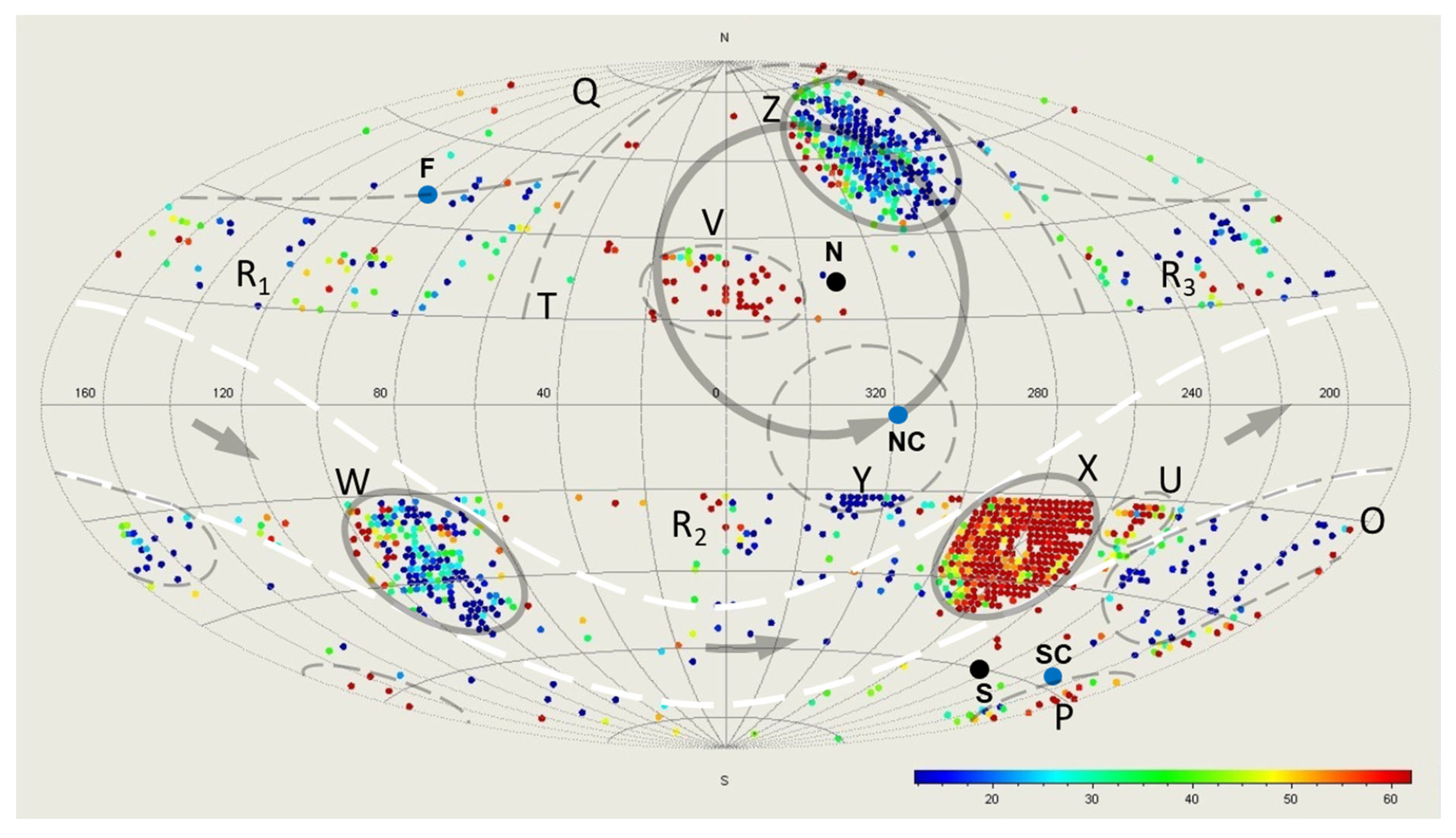
Figure 2.
A schematic diagram of the inner horizon of a spinning host black hole. The elliptical perimeter (black) represents the inner horizon. The ellipse at the center (red) represents the DO. The slashed lines (dark red) represent the emission beams Vb, developing symmetrically about the DO. The dashed curves (dark red) represent the scattered Vb and falling drops of Vb. The horizontal lines (dark red), connecting with the dashed curves, represent the circulating part of the spiral flows Vs. Note that the emission beams Vb, the falling drops of Vb, and the circulating part of the Vs form the circulating flows (dark red), representing the mass-energy that was not immediately immobilized. The horizontal lines (gold) represent the spiral flows Vs of the mass-energy falling from the exterior of the host black hole. The vertical line (black) is the axis of spin.
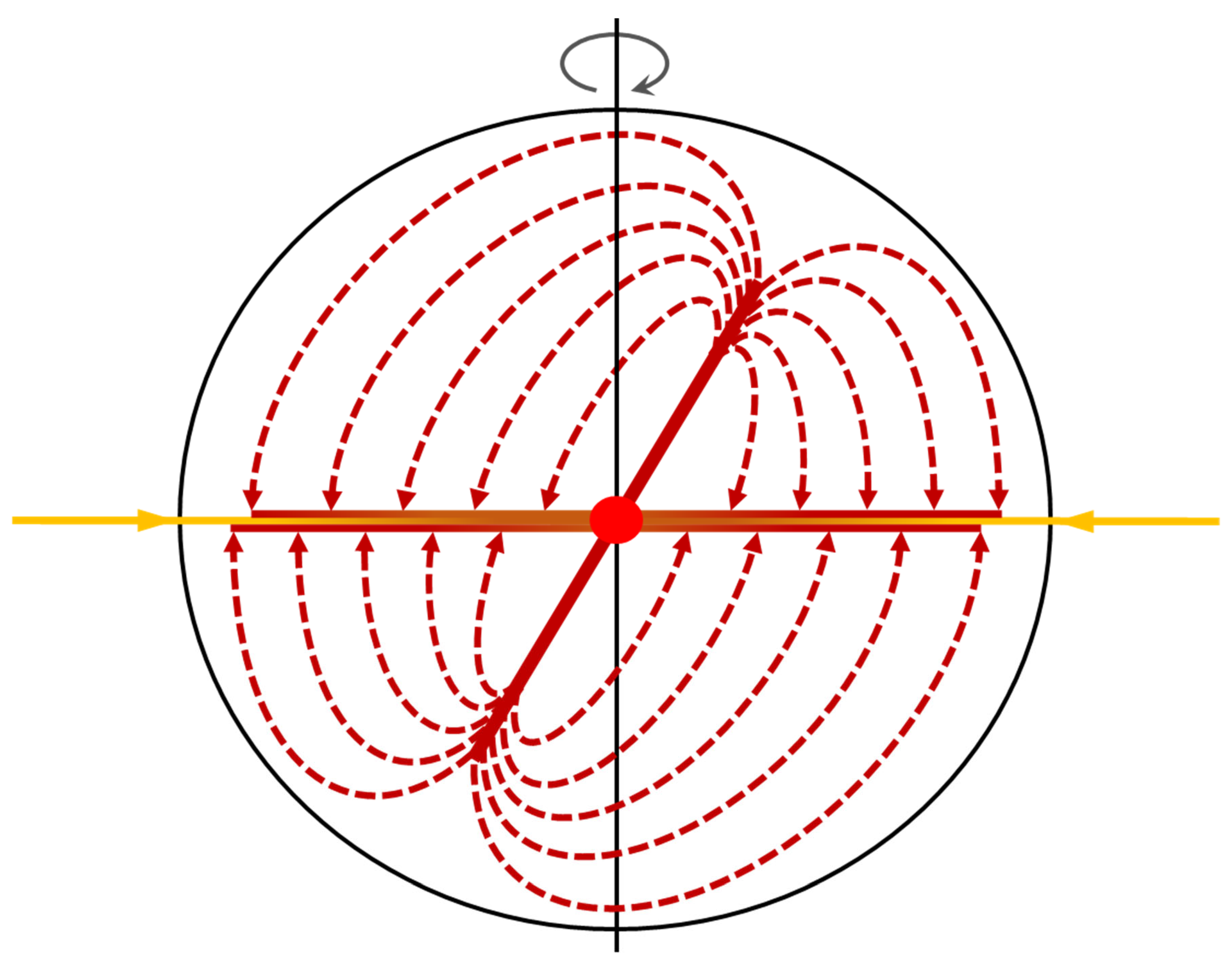
Figure 3.
Large LVC regions. a, hot part; b, cold part of region X. Note the alignment of the dividing plane of the hot and cold parts, the axis of spin (black line NS), and the observer LS (green). c, regions Z and V. The trace of the sweeping Vb on the SLS: clockwise grey arrows; the LVC frontline of sweeping : purple line. d, region W: a temperature dipole. The upper-right end is hotter, and the lower-left end colder. All the LVC coordinates are taken from [4]. The colors used to duplicate the LVC points are: blue (low temperature)-green-light green-yellow-orange-red-purple (high temperature). Other symbols: 3D globe of the SLS (green).
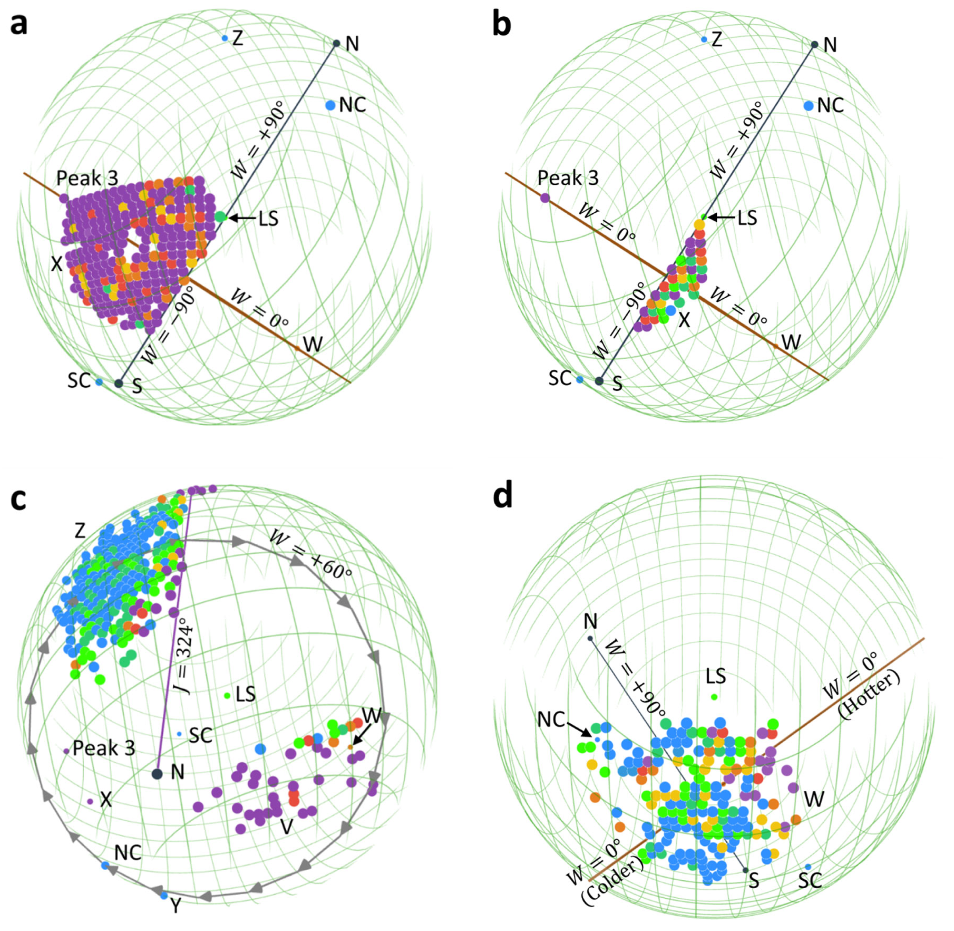
Figure 4.
The Center of the Universe: the intersection (red) of line NC-SC (blue) and the Vs plane (orange) determined by region X, region W, and Peak 3. Other symbols: the LS (green) and 3D globe of the SLS (green).
Figure 4.
The Center of the Universe: the intersection (red) of line NC-SC (blue) and the Vs plane (orange) determined by region X, region W, and Peak 3. Other symbols: the LS (green) and 3D globe of the SLS (green).
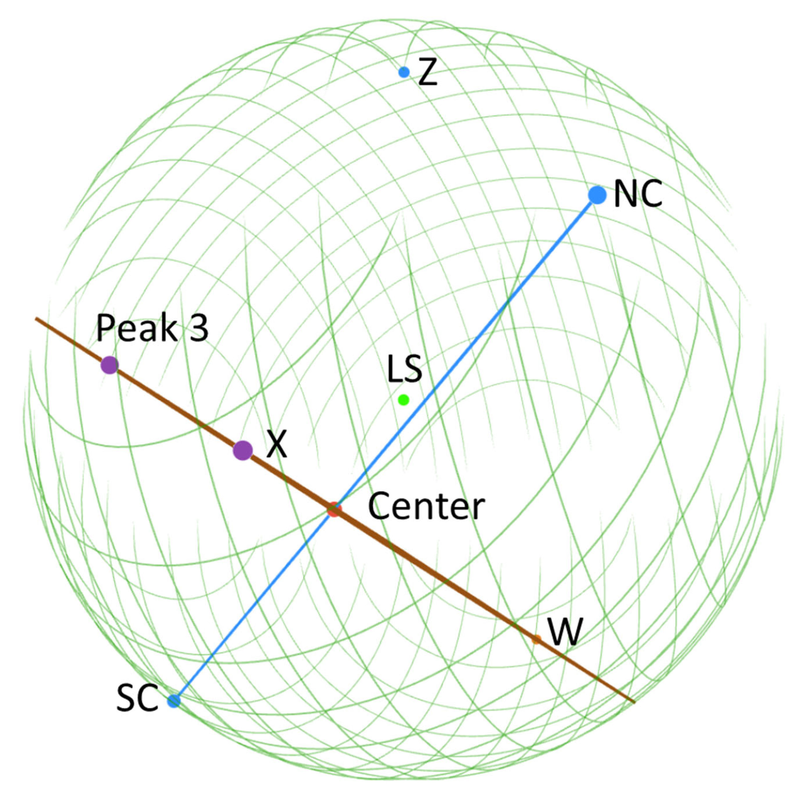
Figure 5.
A schematic picture for the spinning Universe. Note that this figure is not to scale, in particular, the size and eccentricity of the Universe are unknown. The Universe, born from the Center (red dot), spinning about the axis of spin (black line NS), has a rotational energy field: lower (red) close to the axis of spin, higher (blue) far away. The Universe has been veering ellipsoidal (orange ellipse). We in the LS are in the Northern Universe, with a UCS latitude of and a distance of away from the Center. For us, the slowest expansion direction is SED (dark red), pointing towards the axis of spin.
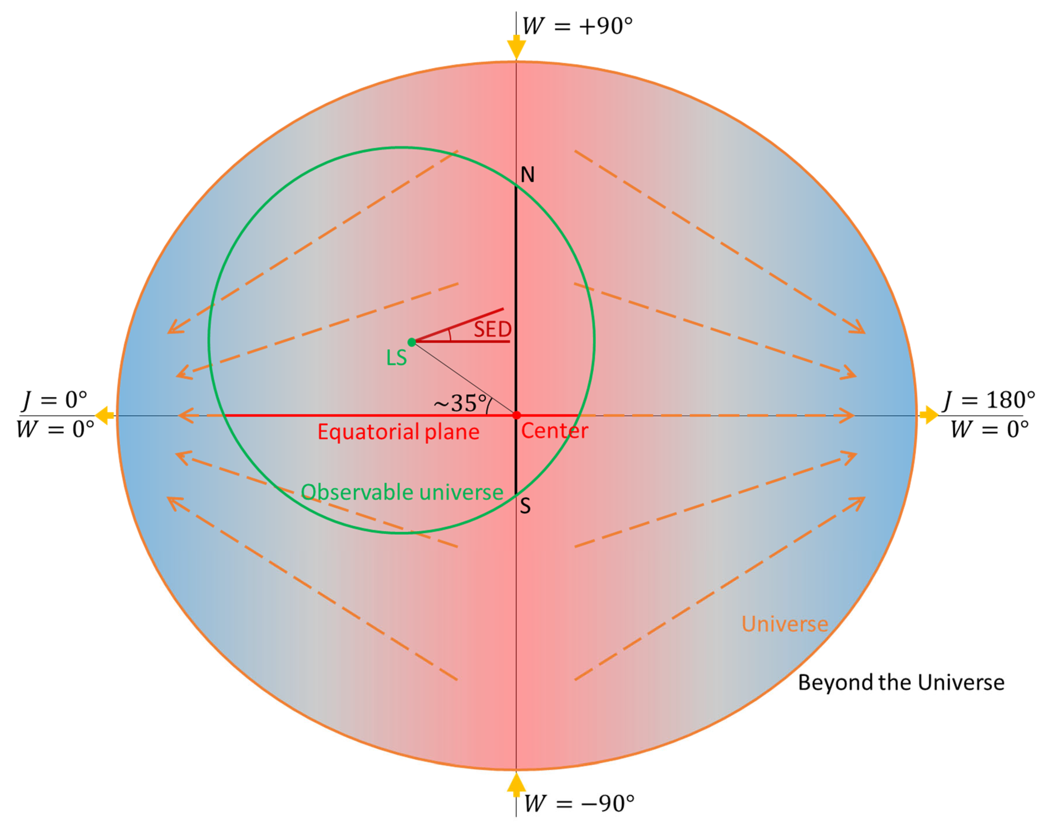
Figure 6.
The sweeping emission beams intersecting the SLS. As the DO spun in the clockwise direction (top view), the emission beams swept the surroundings (represented by the light blue cones) and intersected the SLS (3D green globe). The distance of the intersection to the Center generated by the Northern beam decreased (red solid arrow), while that generated by the Southern beam increased (red dashed arrow, note that this arrow is behind the axis of spin NS). Should the speed of sweeping on the SLS be comparable to that of the emission beams, a long arc or half a loop (along the red solid arrow) could be seen in the CMB. Should the speed of sweeping be much larger than that of the emission beams, loops through NC and SC could be seen. In reality, only an ellipse is observed with a slightly longer axis along the rotation direction at NC, indicating that the speed of sweeping was much smaller than that of the emission beams.
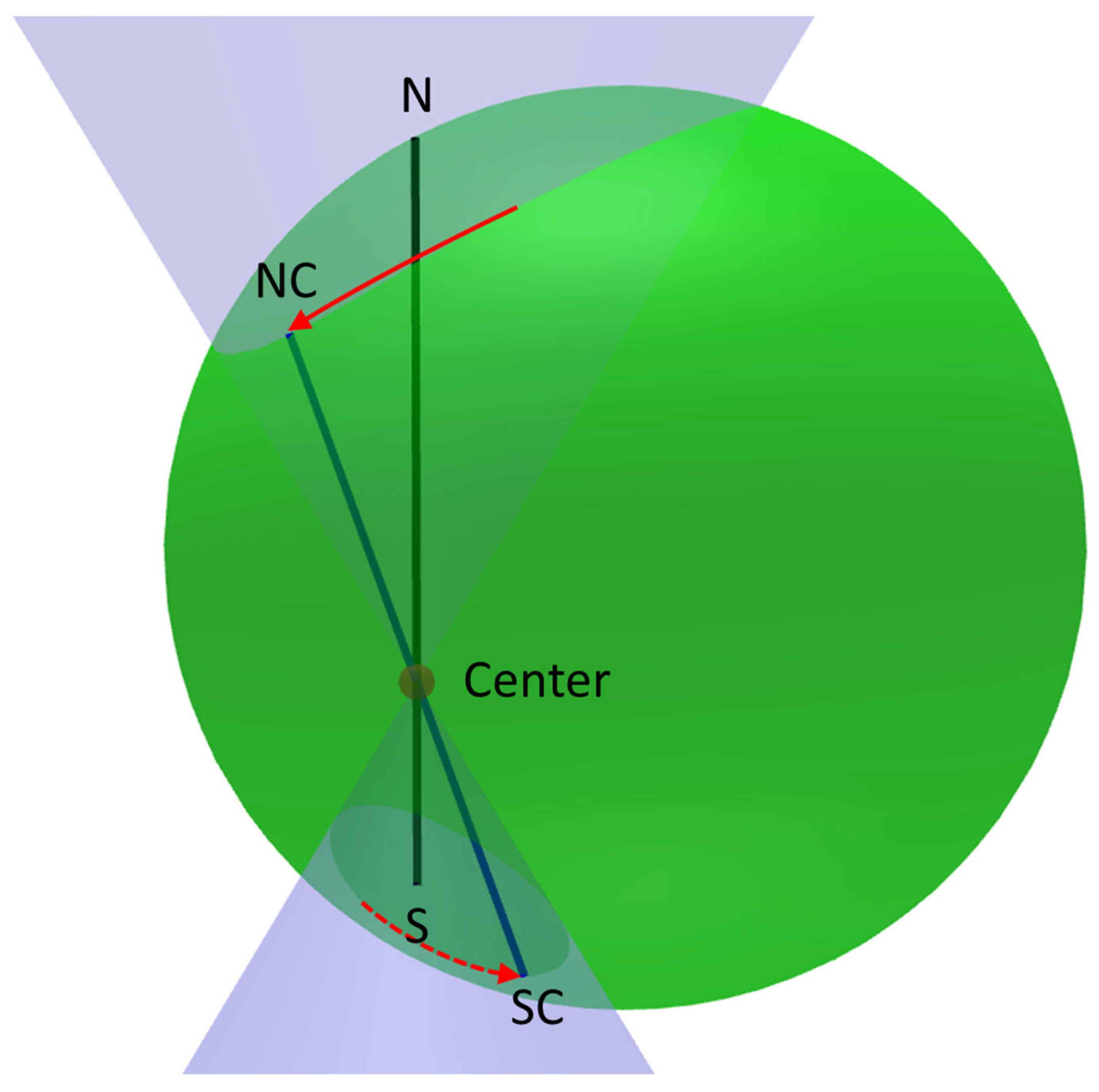
Figure 7.
The observable Hubble constant with respect to the scale factor of the spinning Universe after last scattering (). The parameters: , ,, , and .
Figure 7.
The observable Hubble constant with respect to the scale factor of the spinning Universe after last scattering (). The parameters: , ,, , and .
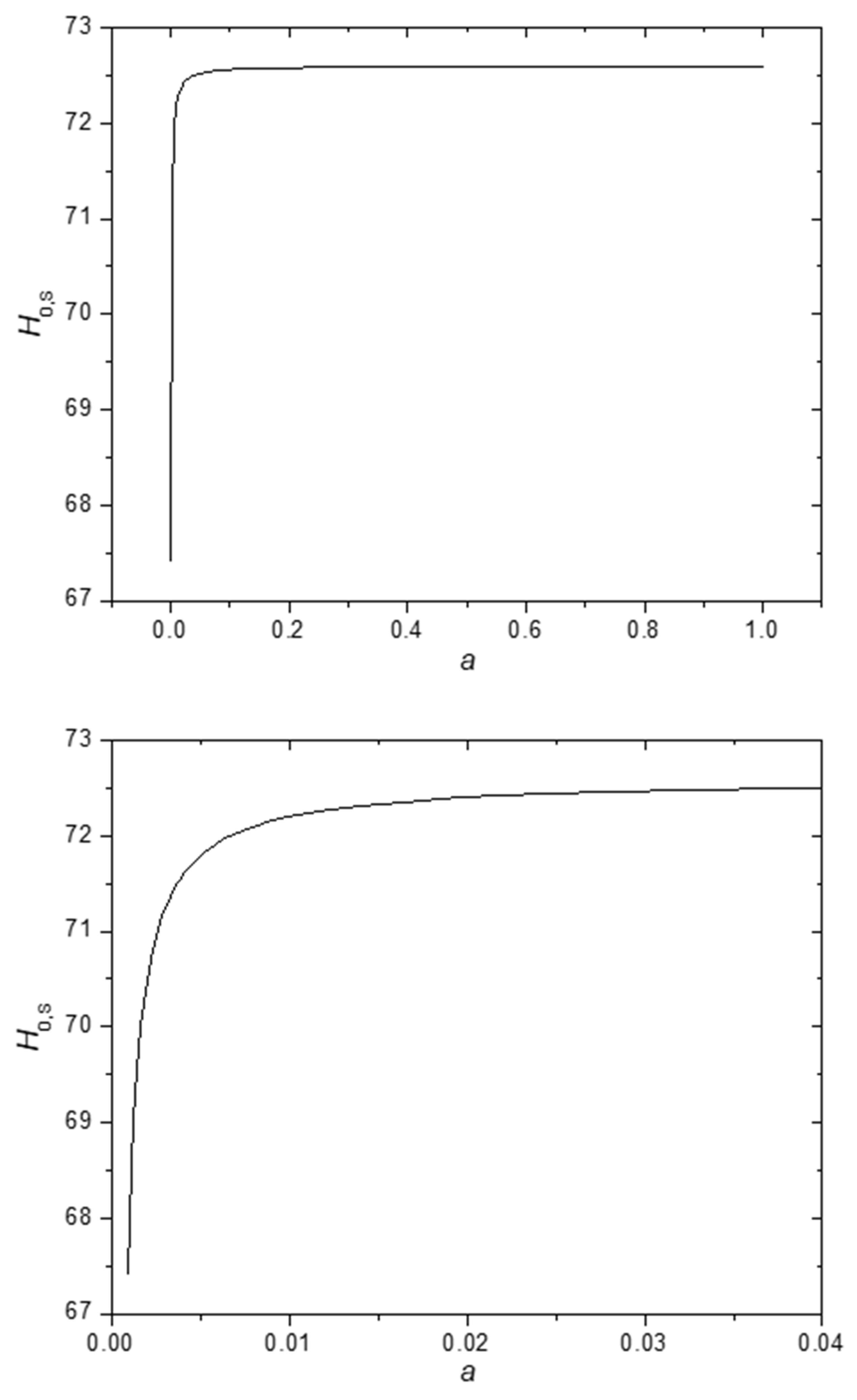
Figure 8.
Unit vectors of the observed SED point towards the axis of spin. a, Side view, parallel to the equatorial plane; b, Top view, along the axis of spin (black line NS). All vectors are plotted in the length of the radius of SLS: CMB dipole (red), galaxy cluster anisotropy (blue), bulk flows (grey), Great Attractor (green), SNe Ia dipole (yellow), dark energy dipole (orange), fine-structure constant dipole (violet). The line (orange) is the rotational plane of the LS (green). Other symbols: 3D globe of the SLS (green).
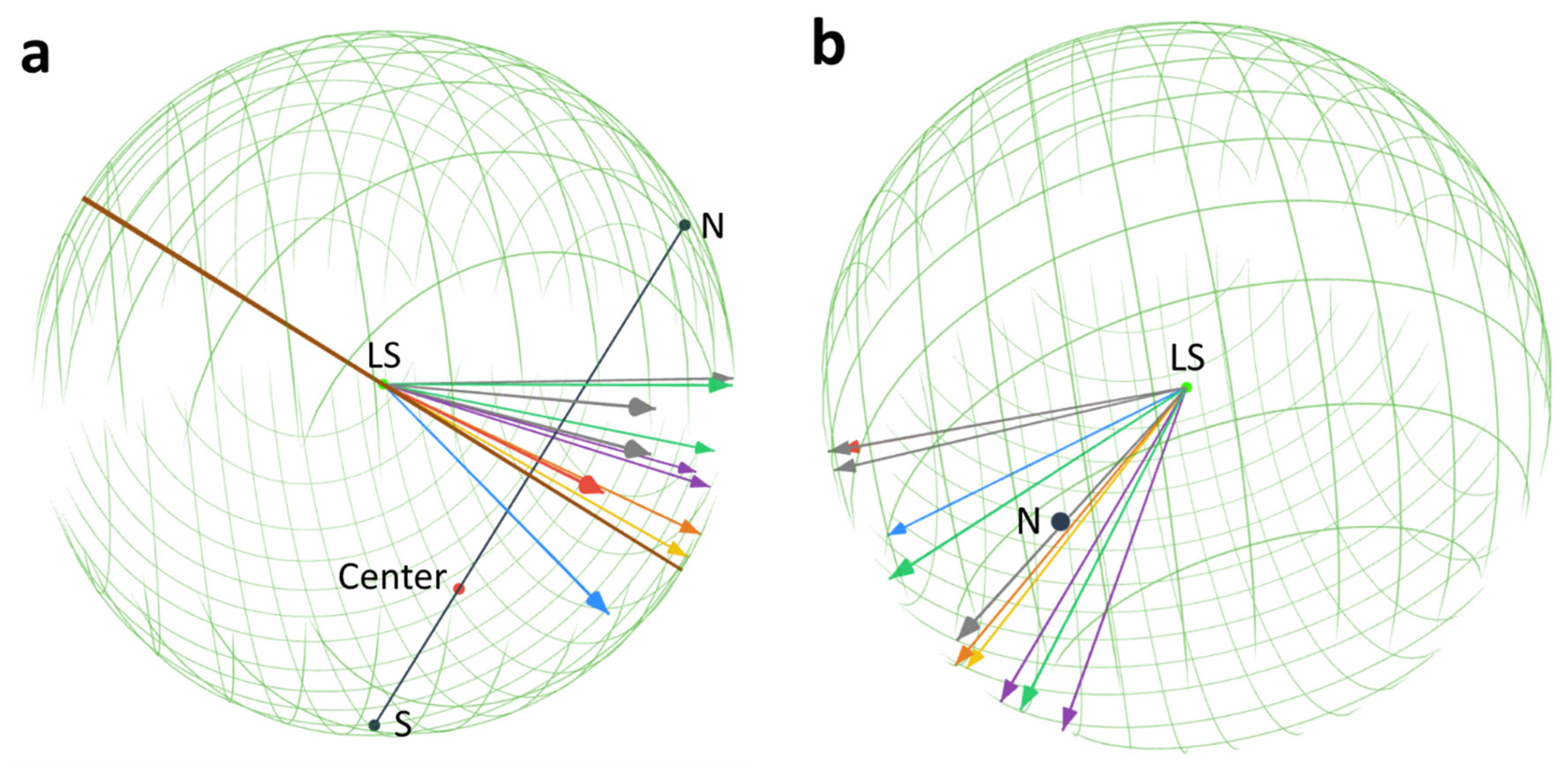
Figure 9.
The spin of the Universe since last scattering. This plot is a projection on the Universal equatorial plane (). We in the LS are at the UCS longitude: , while region W is at . The characteristic pattern of the temperature dipole of region W could be observed only if the observer was in the middle of region W (i.e., the red end peculiarly rotated towards the observer and hence appears hotter, while the blue end peculiarly rotated away from the observer and hence appears colder) at last scattering: , but it is observed by us now: . Therefore, the Universe has spun clockwise through since last scattering so that and can overlap.
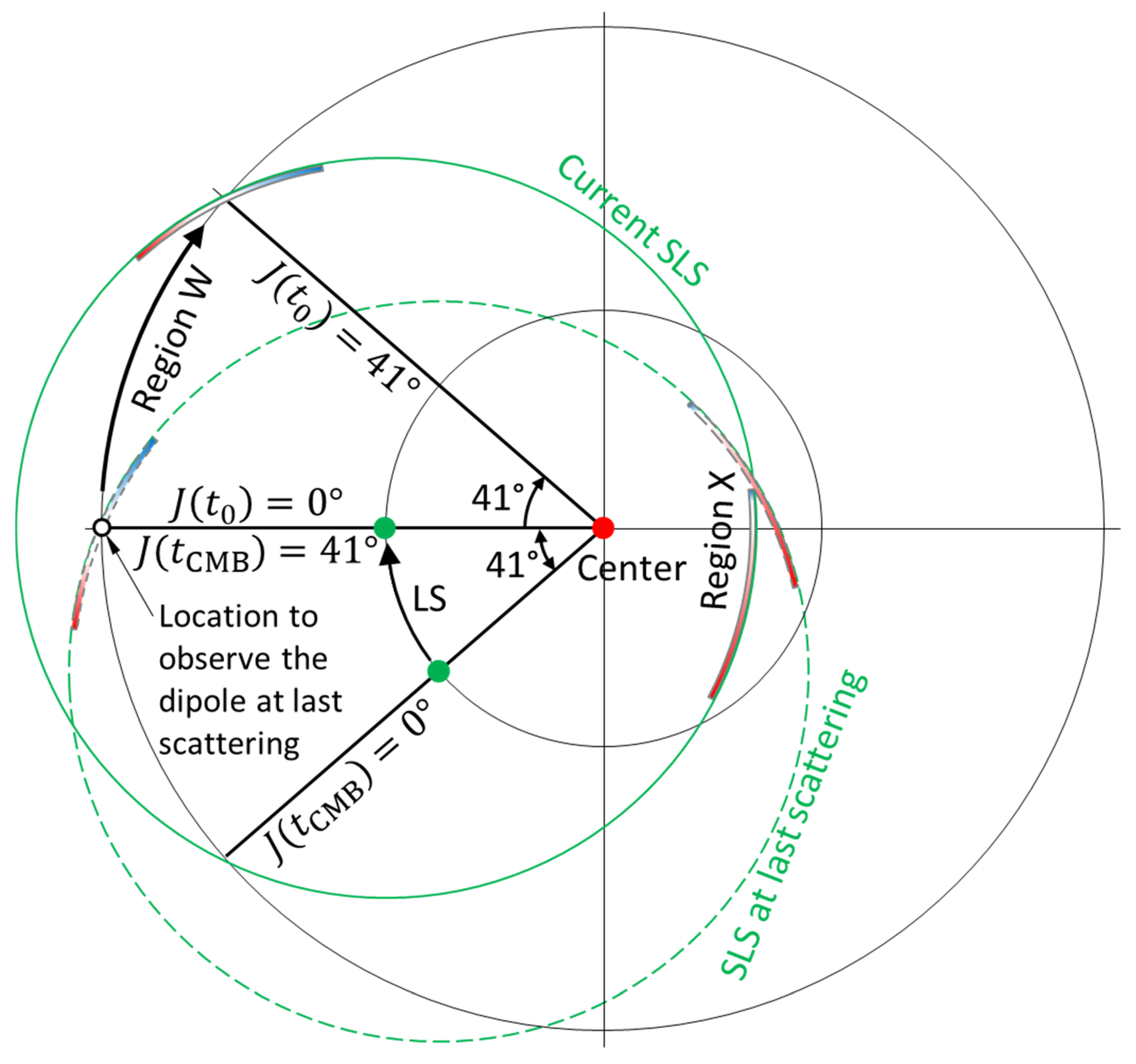
Figure 10.
A schematic diagram of Nature. Before our current Universe, there was a previous aeon (blue), in which there was a host black hole (black ellipses) spinning clockwise. The collapse of its core, the densest object (black dot), generated the Big Bang of our Universe (red). Within our Universe, there are many black holes (black ellipses). As they grow and merge (dashed thin red lines), the masses of the survived black holes increase. Once any one of them exceeds the mass limit of the densest object, a new Big Bang will occur to generate the next aeon (orange). The dot (green) in our Universe represents when and where we are.
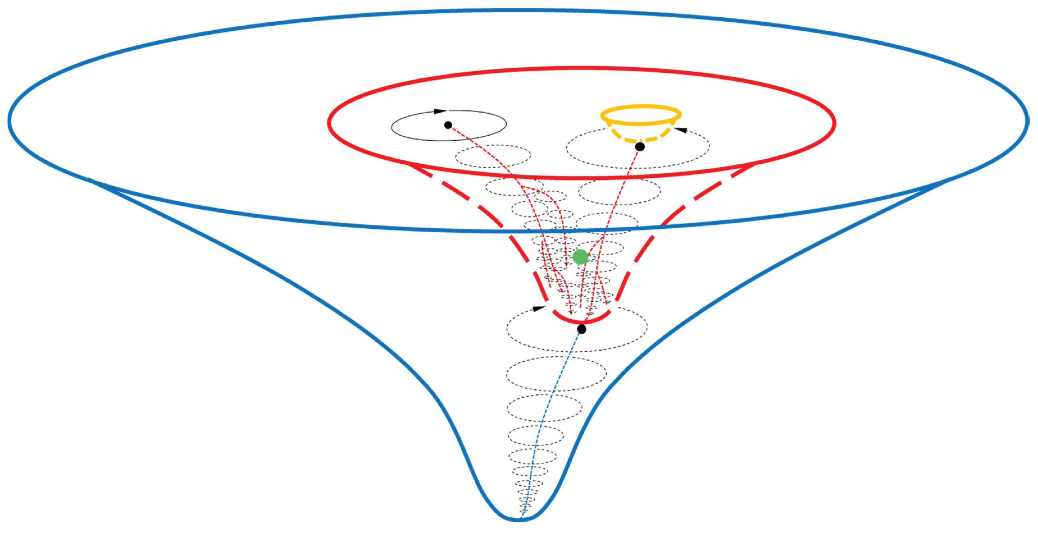

Table 1.
Typical astronomical observations of cosmic anisotropies.
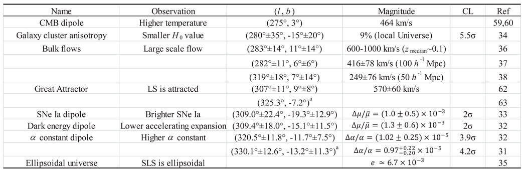 |
a) Converted from the equatorial coordinates.
Disclaimer/Publisher’s Note: The statements, opinions and data contained in all publications are solely those of the individual author(s) and contributor(s) and not of MDPI and/or the editor(s). MDPI and/or the editor(s) disclaim responsibility for any injury to people or property resulting from any ideas, methods, instructions or products referred to in the content. |
© 2025 by the authors. Licensee MDPI, Basel, Switzerland. This article is an open access article distributed under the terms and conditions of the Creative Commons Attribution (CC BY) license (http://creativecommons.org/licenses/by/4.0/).
Copyright: This open access article is published under a Creative Commons CC BY 4.0 license, which permit the free download, distribution, and reuse, provided that the author and preprint are cited in any reuse.


