
Submitted:
22 November 2024
Posted:
25 November 2024
You are already at the latest version
Abstract
Predicting reference evapotranspiration (ETo) is essential for calculating crop water requirements, especially when available data are limited. The goal was to evaluate the daily performance of seven alternative ETo methods (EToalti) and to predict annual accumulated ETo with the standard method of Penman–Monteith with limited data (EToPMP), in the state of Sinaloa, Mexico. From the National Water Commission and the National Meteorological Service (CONAGUA-SMN), daily data were obtained from 11 weather stations in Sinaloa for 1969–2018: maximum temperature, minimum temperature, and evaporation (Eva). Also, from the San Juan CONAGUA–SMN weather station, the following were obtained: wind speed, mean temperature, incident solar radiation, atmospheric pressure, and relative humidity. The seven EToalti calculated were Romanenko (EToRo), Priestley–Taylor (EToPT), McGuinness and Bordne (EToMB), Hargreaves (EToH75), pan Eva (EToTE), Hargreaves (EToH85), and Oudin (EToOu). Daily mean ETo of the data-limited Penman–Monteith method (EToPM) was calculated. The mean absolute error (MAE) and the root mean square error (RMSE) between EToPM and the seven EToalti were calculated. Using multiple linear and nonlinear regressions, EToPMP (dependent variable) was predicted using the seven EToalti (independent variables). In general, the EToalti with the best performance are EToTE (MAE from 0.360 mm day–1 to 2.294 mm day–1 and RMSE from 0.594 mm day−1 to 3.094 mm day–1). The EToalti least recommended are EToMB (MAE from 2.254 mm day−1 to 3.484 mm day–1 and RMSE from 2.948 mm day–1 to 4.437 mm day–1). EToPT was the only EToalti that contributed to the explanation of all models of EToPMP. This study provides mathematical models that can help make agricultural irrigation more efficient in the state considered “the breadbasket of Mexico.”
Keywords:
Penman–Monteith reference evapotranspiration
; alternative methods
; prediction
; limited data
1. Introduction
Reference evapotranspiration (ETo) is an essential variable for hydrological modeling and design of agricultural irrigation [1,2], particularly when data are limited and drought conditions prevail [3,4,5,6]. ETo is the evapotranspiration rate of a hypothetical reference crop 12 cm tall and growing under optimal water conditions [2,7]. At the global level and when all observed variables are available, the standard method for estimating ETo is Penman–Monteith FAO–56 (EToPMO) [8]. However, due to the large number of variables required for its calculation, ETo is usually estimated using alternative methods () [9].
One of the that is recommended in the growth stage of agricultural crops [10,11] is Romanenko (EToRo) [12]; cited by [13]. On the other hand, many authors, e.g., [8,10,11,14] recommend the use of the Priestley–Taylor method (EToPT) [15] due to its high sensitivity and consistency under semi-arid climate conditions. Also, because they only use the variables of mean air temperature (Tmean) and extraterrestrial solar radiation (Ra), the McGuinness and Bordne (EToMB) [16] and Oudin (EToOu) [17] methods can be a good alternative for measuring ETo, particularly when reliable performance is desired [13,18,19]. According to [5,8,11], the Hargreaves method [20,21,22] is a widely used (EToH75 and EToH85) worldwide, because it is an excellent alternative when the only variables available are Tmean, maximum temperature (Tmax), and minimum temperature (Tmin). However, when only evaporation (Eva) data are available, [23] recommends the pan-evaporation method (EToTE), which is an that usually provides good estimates, including low cost and a high simplicity and accuracy. The seven listed above are widely used in underdeveloped countries, such as Mexico, mainly because weather stations usually present three limitations: a) small number of measured variables, b) high percentage of missing data and c) nonhomogeneity of the climate series. These three limitations are not foreign to Sinaloa, which is an eminently agricultural state and has a mostly semi-arid climate [24], so strategies must be developed to calculate EToPMO using the limited data available (EToPM).
In this study, through the National Water Commission and the National Meteorological Service [25], daily data on Tmax, Tmin and Eva were obtained for 11 weather stations in Sinaloa (period 1969–2018). After calculating the complete and homogeneous series of Tmax, Tmin and Eva, Tmean was calculated. Next, ETo was calculated by means of each of the seven described in the second paragraph of this introduction. Based on the equations proposed by [26], EToPM was also calculated. Using the mean absolute error (MAE) and the root mean square error (RMSE), the average daily performance of the seven were calculated. For the MAE and RMSE, the variables were EToPM vs (i=1,…,7) After calculating the annual cumulated value of EToPM at the 11 weather stations, the predicted annual cumulated value of EToPM [EToPMP (dependent variable)] was modeled using multiple linear and nonlinear regressions, where the seven acted as independent variables. The 11 models of EToPMP were validated using the three tests recommended by [24]: a) normality of residuals, b) linearity and fit, and c) homogeneity of residuals. Due to the small number of weather stations, EToPM was validated at only one weather station. This validation consisted of finding a significant correlation in the daily data for the year 2008 between EToPM (Mocorito station) and EToPMO (San Juan station).
The goal of the study is to evaluate the performance of seven and predict EToPMP in the state of Sinaloa, Mexico.
The 11 models of EToPMP contribute an accurate tool to quantify the hydric needs of agricultural crops in Sinaloa [6]. These water needs can provide the basis for the efficient design of irrigation plans, based on the rational use of water resources [27] in a region considered “the breadbasket of Mexico” [24].
2. Materials and Methods
2.1. Study Area
This study was carried out in the state of Sinaloa, located in northwestern Mexico (Figure 1). Although the state covers only 2.9% of the area of Mexico, it is considered the largest producer of vegetables and grains [28], which is why it is called “the breadbasket of Mexico” [29]. According to [30], the climate conditions of Sinaloa range from dry and semi-dry in the coastal plain to temperate and semi-warm-subhumid in the mountain range. Tmean ranges mostly from 14.0 °C to 26.0 °C. The study uses data from 11 weather stations: Culiacán, El Playón, Guatenipa, Ixpalino, La Cruz, Mocorito, Sanalona II, Rosario, Santa Cruz de Alaya, Siqueros and Surutato. An additional station, San Juan was used for validation of the results of Mocorito station (Figure 1).
2.2. Data
Daily data on Tmax, Tmin and Eva were obtained from the 11 weather stations for the period 1969–2018. The data was provided by [25]: https://smn.conagua.gob.mx/es/climatologia/informacion-climatologica/informacion-estadistica-climatologica. [31] also provided data for the year 2008 from San Juan station (located approximately 7.7 km from the Mocorito station): https://smn.conagua.gob.mx/tools/GUI/sivea_v3/sivea.php. The sub-hourly series (every 10 minutes) of data provided for San Juan station were wind speed at a height of 10 m (), observed mean temperature (TmeanO), observed incident solar radiation (SRR), observed atmospheric pressure (PatmO), and observed relative humidity (RHO).
2.2.1. Data Quality Control
The following quality controls were applied to the daily series of Tmax, Tmin and Eva:
- (a)
- To improve the statistical confidence of the results, weather stations containing at least 50 years of available data were chosen.
- (b)
- The missing days were filled in (it was verified that all series recorded 18,262 days); that is, 38 normal years and 12 leap years.
- (c)
- It was verified that Tmax > Tmin and that Eva ≥ 0.
- (d)
- Missing daily data were imputed using the method of interpolation of standardized neighboring series [32].
- (e)
Items d–e were done with the climatol package, version 4.1.0, developed by [35]. After quality control, Tmean was calculated from Tmax and Tmin.
The sub-hourly series from the San Juan station were subjected to three quality controls:
2.3. Reference Evapotranspiration (ETo)
2.3.1. Alternative Methods ()
2.3.1.1. Romanenko (EToRo)
Many methods have been reported in the literature; however, in this study only seven methods are used, which were chosen for their high ease and precision. The first method is Romanenko [12,13,19] (Equation 1).
where: EToRo = Romanenko reference evapotranspiration (mm day–1), Tmean = mean temperature (°C), = actual vapor pressure (kPa) and = saturation vapor pressure (kPa).
Since there are no relative humidity (RH) data from the 11 weather stations, and were calculated using Equations 2 and 3, respectively.
where: Tmin = minimum temperature (°C).
2.3.1.2. Priestley–Taylor (EToPT)
Another method preferred by many authors is Priestley–Taylor [15] (Equation 4), because it is a simplification of the original Penman method [38,39]. The Priestley–Taylor method differs from the Penman method in that the former adds a coefficient, which varies as vegetation, soil moisture and advection also vary.
where: EToPT = Priestley–Taylor reference evapotranspiration (mm day–1), ∆ = slope of the saturated vapor pressure curve (kPa °C–1, calculated from Equation 5), γ = psychrometric constant (kPa °C–1, calculated from Equations 6 and 7), Rn = net radiation (MJ m–2 day–1, calculated from Equations 8–12), G = soil heat flux density (MJ m–2 day–1, null when working at the daily scale) and λ = latent heat of vaporization (2.45 MJ kg–1).
where: Patm = atmospheric pressure (kPa), γO = observed psychrometric constant (kPa °C−1), PatmO = observed atmospheric pressure (kPa) and z = elevation of the weather station (masl).
where: Rnl = net longwave radiation (MJ m–2 day–1), Rns = net shortwave radiation (MJ m−2 day–1), SR = calculated incident solar radiation (MJ m–2 day–1), Ra = extraterrestrial solar radiation (calculated using quadratic polynomials, after obtaining Ra values from [26] (MJ m–2 day–1), SRo = incident solar radiation with clear sky (MJ m–2 day–1), Tmax = maximum temperature (°C), KRS = solar radiation adjustment coefficient (dimensionless, KRS = 0.16 was used in this study), TmeanK = mean temperature (°K4) and σ = Stefan–Boltzmann constant (0.4903 × 10⁻⁸ MJ K–4 m–2 day–1).
2.3.1.3. McGuinness Bordne (EToMB)
2.3.1.4. Hargreaves (EToH75)
2.3.1.5. Pan-Evaporation (EToTE)
In many cases only Eva data are available, so according to [40], the pan-evaporation method [41] (Equation 15) can be a good alternative for estimating ETo.
where: EToTE = pan-evaporation reference evapotranspiration (mm day–1), Eva = evaporation of water from the pan (placed in a dry fallow area; mm day–1) and = tabulated adjustment coefficient. depends on RH (%, calculated using Equation 16), approximate distance between the crop and the weather station (considered in this study to be 100 m) and = wind speed at a height of 2 m (m s–1, considered in this study to be 2 m s–1) [26,41].
In this study = 2 m s–1 was applied because it is a value recommended by [26] when observed data are not available. In addition, the same value of was also obtained for 2000 weather stations around the world [26]; cited by [42]). Finally, many authors; for example, [43,44,45], point out that has a marginal impact on the value of EToPM compared to Tmean and SR.
where: RH = relative humidity (%).
2.3.1.6. Hargreaves (EToH85)
2.3.1.7. Oudin (EToOu)
2.3.2. Standard Method
2.3.2.1. Penman–Monteith
Penman–Monteith (Equation 19) is the universal standard method [39], and due to its high precision for measuring ETo of short grass and alfalfa [26], it is the most recommended worldwide.
where: EToPM = Penman–Monteith reference evapotranspiration with limited data (mm day−1) and = daily wind speed at a height of 2 m (m s–1).
2.4. Performance Metrics Between the Seven Alternative Methods () and the Penman–Monteith Method with Limited Data (EToPM)
2.4.1. Mean Absolute Error (MAE) and Root Mean Square Error (RMSE)
Using two performance metrics, mean absolute error (MAE; Equation 20) and root mean square error (RMSE; Equation 21), the performance of the seven was calculated.
where: MAE = mean absolute error (mm day–1), RMSE = root mean square error (mm day−1), = reference evapotranspiration for alternative method i (mm day–1), and = Penman–Monteith reference evapotranspiration with limited data (mm day–1).
2.5. Predictive models of Penman–Monteith Annual Cumulative Reference Evapotranspiration with Limited Data (EToPMP)
First, the annual cumulative value of EToPM was calculated. Multiple linear and non-linear regressions were applied to all series of EToPM. EToPM was transformed into EToPMP (dependent variable) and the seven were the independent variables.
2.6. Validation
2.6.1. Predictive Models of Penman–Monteith Annual Cumulative Reference Evapotranspiration with Limited Data (EToPMP)
The following validations were applied to the residuals of all multiple regressions (linear and non-linear):
- (a)
- Normality: the Shapiro–Wilk test was applied to the residuals of the linear regressions.
- (b)
- If the residuals of the linear regressions were normal, the model was considered validated, otherwise, a non-linear regression (square polynomial) was applied.
- (c)
- Homogeneity: the nullity of the averages of the residuals of all regressions (linear and non-linear) was verified.
- (d)
- Linearity and fit: a correlation hypothesis test was designed (Equations 22 and 23), where the goodness of fit of the models was evaluated. All linear regressions showed linearity: Pearson correlation (Pr) ≥ Pearson critical correlation (|Pcr|) [(|Pcr| = 0.279; n = 50)]. All non–linear regressions showed good fit: Spearman correlation (Sr) ≥ Spearman critical correlation (|Scr|) [(|Scr| = 0.280; n = 50)]. In all models, Pr and Sr were obtained using √R2.
2.6.2. Penman–Monteith Daily Reference Evapotranspiration with Limited Data (EToPM)
At San Juan station, using Equation 24, the average daily wind speed was determined at a height of 2 m.
where: = average daily wind speed measured at a height of 10 m (m s–1) and z = measurement height of (m).
Because San Juan station also presented PatmO and RHO data, and the observed saturation vapor pressure () were calculated with Equations 7 and 25, respectively:
where: = observed saturation vapor pressure (kPa) and RHO = observed relative humidity (%).
Finally, for the San Juan station data, a dispersion analysis was applied between EToPM vs EToPMO (calculated with Equations 2, 5, 7–12 and 24–26). After a normality analysis, it was found that Pr ≥ |Pcr| (|Pcr| = 0.103; n = 366 for the year 2008).
where: EToPMO = Penman–Monteith observed reference evapotranspiration (mm day–1) and TmeanO = observed mean temperature (°C).
2.7. Software Used and Significance of Statistical Analysis
To carry out this study, the following programs were used: Office 365, XLstat version 2024, RStudio version 2023.12.1 build 402, Past 4.02 and CorelDRAW version 2019.
All statistical analyses were performed with a statistical significance of α = 0.05.
3. Results
3.1. Variation of the Temperatures Maximum (Tmax), Minimum (Tmin) and Mean (Tmean), and the Evaporation (Eva)
According to Table 1, the average, maximum. and minimum values recorded the following ranges: for Tmax from 24.995 °C (Surutato) to 34.633 °C (Guatenipa), from 37.500 °C (Surutato) to 47.000 °C (Guatenipa) and from 9.000 °C (Mocorito and Surutato) to 18.000 °C (Ixpalino), respectively. For Tmin, from 7.257 °C (Surutato) to 19.545 °C (Culiacan), from 20.500 °C (Surutato) to 37.000 °C (El Playón) and from –6.000 °C (Surutato and El Playón) to 2.000 °C (Culiacan), respectively. For Tmed, from 16.126 °C (Surutato) to 26.230 °C (Culiacán), from 27.500 °C (Surutato) to 38.000 °C (Guatenipa) and from 2.300 °C (Surutato) to 12.750 °C (Rosario), respectively. For Eva, from 3.976 mm (Surutato) to 6.648 mm (El Playón), from 12.500 mm (Surutato) to 17.900 mm (Culiacán) and from 0.000 mm (Culiacán, Guatenipa, La Cruz, Sanalona II, Rosario, Santa Cruz de Alaya, Siqueros and Surutato) to 0.100 mm (El Playón and Ixpalino).
3.2. Average Daily Reference Evapotranspiration (ETo) Estimated Using Seven Alternative Methods () and the Penman–Monteith Method with Limited Data (EToPM)
As shown in Table 2, recorded the following ranges: for EToH85, from 2.987 mm day–1 (December in La Cruz) to 7.798 mm day–1 (May in Guatenipa); for EToH75. from 2.806 mm day–1 (December in La Cruz) to 6.877 mm day–1 (May in Ixpalino); for EToPT. from 1.920 mm day–1 (December in El Playón) to 6.767 mm day–1 (May in Guatenipa); for EToTE. from 1.521 mm day–1 (December in La Cruz) to 6.554 mm day–1 (June in El Playón). For as shown in Table 2, ranges were recorded for EToMB from 3.131 mm day–1 (December in El Playón) to 8.710 mm day–1 (June in Guatenipa); for EToRo, from 5.959 mm day–1 (December in La Cruz) to 10.972 (May in Guatenipa); and for EToOu, from 2.129 mm day–1 (December in El Playón) to 5.923 mm day–1 (June in Guatenipa). The standard method (EToPM) ranged from 2.071 mm day–1 (December in La Cruz) to 4.321 mm day–1 (May in Guatenipa).
, as shown in Table 3, recorded the following ranges: for EToH85, from 2.533 mm day–1 (December in Surutato) to 7.494 mm day–1 (May in Sanalona II); for EToH75. from 2.379 mm day–1 (December in Surutato) to 7.038 mm day–1 (May in Sanalona II); for EToPT, from 1.553 mm day–1 (December in Surutato) to 6.338 mm day–1 (May in Sanalona II); for EToTE, from 1.217 mm day–1 (December in Surutato) to 5.396 mm day–1 (May in Sanalona II). Table 3 also shows the following ranges: for EToMB, from 2.049 mm day–1 (December in Surutato) to 8.553 mm day−1 (June in Mocorito); for EToRo, from 5.081 mm day–1 (January in Surutato) to 10.390 (May in Sanalona II); and for EToOu, from 1.393 mm day–1 (December in Surutato) to 5.816 mm day–1 (June in Mocorito). The standard method (EToPM) ranged from 1.929 mm day–1 (December in Surutato) to 4.221 mm day–1 (May in Sanalona II). In Mocorito station, no Eva data were recorded for any day in the period 1969–2018.
3.3. Performance Metrics Comparing the Seven Alternative Methods () with the Penman–Monteith Method with Limited Data (EToPM)
In general, the with best performance for summer (June–August) was EToTE (Figure 2), as MAE ranged from 0.399 mm day–1 (August in Guatenipa; Figure 2e) to 2.294 mm day−1 (June in El Playón; Figure 2c) and RMSE ranged from 0.636 mm day–1 (August in Guatenipa; Figure 2f) to 3.094 mm day–1 (June in El Playón; Figure 2d). For winter (December–February) the with the best performance was EToOu, since MAE ranged from 0.244 mm day–1 (February in El Playón; Figure 2c) to 0.386 mm day−1 (January in Ixpalino; Figure 2g) and RMSE ranged from 0.395 mm day–1 (December in El Playón; Figure 2d) to 0.561 mm day–1 (February in Culiacán; Figure 2b). The with the lowest performance for summer was EToMB, since MAE ranged from 2.920 mm day–1 (June in Guatenipa; Figure 2e) to 3.484 mm day–1 (July in El Playón; Figure 2c) and RMSE ranged from 3.773 mm day–1 (August in Guatenipa; Figure 2f) to 4.437 mm day–1 (July in El Playón; Figure 2d). The with the lowest performance for winter was EToRo, since MAE ranged from 2.095 mm day–1 (July in El Playón; Figure 2c) to 3.447 mm day–1 (June in Guatenipa; Figure 2e) and RMSE ranged from 2.367 mm day–1 (July in La Cruz; Figure 2j) to 4.538 mm day–1 (June in Guatenipa; Figure 2f).
In Figure 3, the that performed best for summer was EToTE, because MAE ranged from 0.360 mm day–1 (August in Siqueros; Figure 3i) to 1.238 mm day–1 (June in Santa Cruz de Alaya; Figure 3g) and RMSE ranged from 0.594 mm day–1 (August in Siqueros; Figure 3j) to 1.745 mm day–1 (June in Santa Cruz de Alaya; Figure 3h). For winter, the with the best performance was EToOu, since MAE ranged from 1.023 mm day–1 (June in Surutato; Figure 3k) to 1.752 mm day–1 (July in Rosario; Figure 3e) and RMSE ranged from 1.386 mm day–1 (June in Surutato; Figure 3l) to 2.110 mm day–1 (July in Mocorito; Figure 3b). The minimum performance in summer was recorded for EToMB, since MAE ranged from 2.254 mm day–1 (June in Surutato; Figure 3k) to 3.356 mm day–1 (July in Rosario; Figure 3e) and RMSE ranged from 2.948 mm day–1 (June in Surutato; Figure 3l) to 4.271 mm day–1 (July in Rosario; Figure 3f). The minimum performance in the winter season was for EToRo, since MAE ranged from 1.894 mm day–1 (February in Surutato; Figure 3k) to 3.691 mm day–1 (December in Santa Cruz de Alaya; Figure 3g) and RMSE ranged from 2.530 mm day–1 (January in Surutato; Figure 3l) to 4.086 mm day–1 (December in Sanalona II; Figure 3d).
3.4. Predictive Models of Penman–Monteith Annual Cumulative Reference Evapotranspiration with Limited Data (EToPMP)
Eleven predictive models were created (five linear and six non-linear). The linear models represented the stations Culiacán, El Playón, Guatenipa, Mocorito and Siqueros (Equations 27–29, 32 and 36, respectively). Nonlinear models corresponded to the stations Ixpalino, La Cruz, Sanalona II, Rosario, Santa Cruz de Alaya and Surutato (Equations 30, 31, 33–35 and 37, respectively). EToPT was the only independent variable that was repeated in all 11 models. The seven contributed to the explanation of all the nonlinear models of EToPMP.
3.5. Validation
3.5.1. Predictive Models of Penman–Monteith Annual Cumulative Reference Evapotranspiration with Limited Data (EToPMP)
3.5.1.1. Normality of Residuals
In Table 4, the normality of the residuals from the multiple linear regressions ranged from W = 0.891 (Ixpalino) to W = 0.983 (Mocorito), and from p(normal) = 0.001 (Ixpalino, La Cruz and Sanalona II) to p(normal) = 0.662 (Mocorito). The residuals that did not present normality [p(normal) < 0.05] were from Ixpalino, La Cruz, Sanalona II, Rosario, Santa Cruz de Alaya and Surutato.
3.5.1.2. Linearity and Fit
All linear regressions showed linearity (|Pr| 0.279) and all non-linear regressions showed good fit (|Sr| > 0.280). Specifically, the linear regressions yielded correlations from Pr = 0.997 in El Playón (Figure 4b) and Guatenipa (Figure 4c) to Pr = 0.999 in Culiacán (Figure 4a), Mocorito (Figure 4f) and Siqueros (Figure 4j). All non-linear regressions recorded a value of Sr = 0.999 [Ixpalino (Figure 4d), La Cruz (Figure 4e), Sanalona II (Figure 4g), Rosario (Figure 4h), Santa Cruz de Alaya (Figure 4i) and Surutato (Figure 4k)].
3.5.1.3. Homogeneity of Residuals
Nearly all residual averages (linear and non-linear regressions) were null (Figure 5). Specifically, residual averages ranged from –0.003 mm year–1 (Rosario; Figure 5h) to 0.001 mm year–1 (La Cruz and Surutato; Figure 5e and Figure 5k, respectively). The completely homogeneous residuals (0.000 mm year–1) were recorded in Culiacán, El Playón, Guatenipa, Ixpalino, Mocorito, Sanalona II, Santa Cruz de Alaya and Siqueros (Figure 5a–d,f,g,i and j; respectively).
3.5.2. Spearman Correlation (Sr) Between Daily Penman–Monteith Reference Evapotranspiration and Limited Data In Mocorito (EToPM), and Observed Data in San Juan (EToPMO)
After checking that only one series presented normality; EToPM [W = 0.996; p(normal) = 0.436] and EToPMO [W = 0.894; p(normal) < 0.001] (Figure 6), a measure of dispersion was applied to calculate the significant correlation between the two series (Sr = 0.265; |Scr |= 0.103 for n = 366∴ Sr > |Scr|).
4. Discussion
The results in Table 1 are similar to those reported by [30], because these authors state that Tmean in Sinaloa ranges mostly from 24.000 °C to 26.000 °C, where areas with higher elevation, such as Surutato (1460 masl), record ranges from 14.000 °C to 20.000 °C. Eva variation of this study (Table 1) registers similarities to the results reported by [46], since these authors indicate that the average monthly of Eva for Sinaloa ranged from 98.720 mm month–1 in December (3.185 mm day–1) to 267.830 mm month–1 in May (8.640 mm day−1). In addition, [46,47] also agree that the highest magnitudes of Eva in Sinaloa occur in the spring (March–May)–summer agricultural cycle.
EToTE results of this study (Table 2 and Table 3) also present similarities with the results reported by [46], since these authors indicate that the average monthly magnitudes of EToTE in Sinaloa ranged from 89.840 mm month–1 in December (2.898 mm day–1) to 222.300 mm month–1 in May (7.171 mm day–1). The variation in EToPM (Table 2 and Table 3) is also consistent with that reported by [48], since according to these authors, EToPM in Culiacán for the year 2020 ranged from 1.600 mm day–1 in February to 10.300 mm day–1 in September. In addition to the above, the highest magnitudes of and EToPM (Table 2 and Table 3) are consistent with [49], who states that the highest percentages of accumulated annual EToH85, for the period 1969–2018 and for the stations Culiacán (60.16%), El Varejonal (60.780%), Ixpalino (59.650%), La Concha (59.250%), Rosario (59.500%), Sanalona II (60.280%), and Santa Cruz de Alaya (59.820%) occur in the spring–summer agricultural cycle.
In general, in this study, EToTE showed better performance for summer than EToPT (Figure 2 and Figure 3). Although [8] did not analyze EToTE, these authors point out that EToPT records better performance than EToH85, since they state that in a region of India the RMSE ranged from 0.770 mm day–1 (EToH85) to 3.120 mm day–1 (EToPT). These differences in performance of EToH85 and EToPT may be because in Sinaloa the radiation-based models are more stable than the temperature-based models [50,51]. On the other hand, [52] calculated the performances for three (EToPT, EToH85 and EToRo) for Manitoba, Canada, finding the following performances, respectively: MAE = 0.362 mm day–1 and RMSE = 0.516 mm day−1, MAE = 0.514 mm day–1 and RMSE = 0.651 mm day–1, and MAE = 0.534 mm day–1 and RMSE = 0.701 mm day–1. That is, the performance results of [52] are consistent with those of this study, since in winter, EToRo recorded the lowest performances and EToPT recorded higher performance than EToH85 (Figure 2 and Figure 3). Another investigation that is consistent with the findings of this study is that of [53], since these authors point out that in the state of Mexico, the average annual RMSE for the period 2003–2008 ranged from 0.442 mm day–1 (EToPT for 2008) to 0.873 mm day–1 (EToH85 in 2007). [13] also agree on two aspects: EToOu is the model with the best performance (MAE = 1.100 mm day–1 and RMSE = 1.440 mm day–1) and EToRo has the lowest performance (MAE = 2.660 mm day–1 and RMSE = 2.960 mm day–1).
[54] note that when generating predictions of EToPMP, specification errors should always be minimized by validating the models [24]. Models 27–29, 32 and 36 (Table 4) were initially validated by the normality of the residuals [p(normal) > 0.05] [55]; and for linearity [56] (Pr > |Pcr|; Figure 4a–c,f y j). In all models where the residuals did not present normality (Table 4; Equations 30, 31, 33–35 and 37), the fit was checked using Sr > |Scr| (Figure 4d,e,g–i and k) [24]. The 11 models proposed in this study recorded homogeneity in the residuals (Figure 5) [56,57]. The method for calculating EToPM was validated using Sr > |Scr| [58].
5. Conclusions
Although Sinaloa is an eminently agricultural state, in many cases complete climate series are not available, which makes the use of and the modeling of EToPMP particularly effective. In general, EToTE is the best performing for summer and autumn (September–November), and EToOu is the best performing for winter. Due to poorer fit in summer, the use of EToMB and EToRo is not recommended for data from Sinaloa weather stations. This study creates 11 predictor models of EToPMP, where seven serve as explanatory variables. EToPT is the only that contributes to the explanation of all EToPMP models. The use of EToPMP can help minimize errors of overestimation and underestimation of crop water needs, which in turn can ensure the hydro-agricultural needs of Sinaloa and Mexico. This is the case since often, particularly under abnormally dry conditions, agricultural irrigation is not properly scheduled and designed, thus undermining the quality and quantity of water for crops.
Author Contributions
Conceptualization, L.C.O.; methodology, L.C.O., N.C.M, P.G.E., A.D.J.A. and A.G.M.A; software, G.A. and P.G.R.E.; validation, L.C.O.; data curation, G.A. and P.G.R.E.; writing—original draft preparation, L.C.O. All authors agree with the current version of the manuscript.
Funding
This research received no external funding.
Data Availability Statement
https://smn.conagua.gob.mx/es/climatologia/informacion-climatologica/informacion-estadistica-climatologica (accessed on 16 July 2024), https://smn.conagua.gob.mx/tools/GUI/sivea_v3/sivea.php (accessed on 22 August 2024).
Acknowledgments
To the Research and Postgraduate Secretariat of the National Polytechnic Institute (SIP–IPN), for financial support for the research project SIP20240953.
Conflicts of Interest
The authors declare no conflicts of interest.
References
- Matsui, H.; Osawa, K. Alternative net longwave radiation equation for the FAO Penman–Monteith evapotranspiration equation and the Penman evaporation equation. Theor. Appl. Climatol. 2023, 153, 1355–1360. [Google Scholar] [CrossRef]
- Kim, C.G.; Lee, J.; Lee, J.E.; Chung, I.M. Calibration and Evaluation of Alternative Methods for Reliable Estimation of Reference Evapotranspiration in South Korea. Water 2024, 16, 2471. [Google Scholar] [CrossRef]
- Elbeltagi, A.; Nagy, A.; Mohammed, S.; Pande, C.B.; Kumar, M.; Bhat, S.A.; Zsembeli, J.; Huzsvai, L.; Tamás, J.; Kovács, E.; Harsányi, E.; Juhász, C. Combination of Limited Meteorological Data for Predicting Reference Crop Evapotranspiration Using Artificial Neural Network Method. Agronomy 2022, 12, 516. [Google Scholar] [CrossRef]
- Fang, S.L.; Lin, Y.S.; Chang, S.C.; Chang, Y.L.; Ysai, B.Y.; Kuo, B.J. Using Artificial Intelligence Algorithms to Estimate and Short-Term Forecast the Daily Reference Evapotranspiration with Limited Meteorological Variables. Agriculture 2024, 14, 510. [Google Scholar] [CrossRef]
- Matimolane, S.; Strydom, S.; Mathivha, F.I.; Chikoore, H. Evaluating the spatiotemporal patterns of drought characteristics in a semi-arid region of Limpopo Province, South Africa. Environ. Monit. Assess. 2024, 196, 1062. [Google Scholar] [CrossRef]
- Sutanto, S.J.; Zarzoza, M.S.B.; Supit, I.; Wang, M. Compound and cascading droughts and heatwaves decrease maize yields by nearly half in Sinaloa, Mexico. npj Nat. Hazards 2024, 1, 26. [Google Scholar] [CrossRef]
- Skhiri, A.; Ferhi, A.; Bousselmi, A.; Khlifi, S.; Mattar, M.A. Artificial Neural Network for Forecasting Reference Evapotranspiration in Semi-Arid Bioclimatic Regions. Water 2024, 16, 602. [Google Scholar] [CrossRef]
- Raja, P.; Sona, F.; Surendran, U.; Srinivas, C.V.; Kannan, K.; Madhu, M.; Mahesh, P.; Annepu, S.K.; Ahmed, M.; Chandrasekar, K.; Suguna, A.R.; Kumar, V.; Jagadesh, M. Performance evaluation of different empirical models for reference evapotranspiration estimation over Udhagamandalm, The Nilgiris, India. Sci. Rep. 2024, 14, 12429. [Google Scholar] [CrossRef] [PubMed]
- Song, X.; Lu, F.; Xiao, W.; Zhu, K.; Zhou, Y.; Xie, Z. Performance of 12 reference evapotranspiration estimation methods compared with the Penman–Monteith method and the potential influences in northeast China. Meteorol. Appl. 2018, 26, 83–96. [Google Scholar] [CrossRef]
- Celestin, S.; Qi, F.; Li, R.; Yu, T.; Cheng, W. Evaluation of 32 Simple Equations against the Penman–Monteith Method to Estimate the Reference Evapotranspiration in the Hexi Corridor, Northwest China. Water 2020, 12, 2772. [Google Scholar] [CrossRef]
- Uzunlar, A.; Dis, M.O. Novel Approaches for the Empirical Assessment of Evapotranspiration over the Mediterranean Region. Water 2024, 16, 507. [Google Scholar] [CrossRef]
- Romanenko, V.A. Computation of the autumn soil moisture using a universal relationship for a large area, Proc. Ukrainian Hydrometeorological Research Institute, 1961. Kiev. No. 3.
- 13. Vásquez, M.R.; Ventura, R.E.J.; Acosta, G.J.A. Habilidad de estimación de los métodos de evapotransporación para una zona semiárida del centro de México. Rev. Mexicana cienc. agric. 2011, 2, 399–415. https://www.scielo.org.mx/scielo.php?script=sci_arttext&pid=S2007-09342011000300008.
- Gao, F.; Feng, G.; Ouyang, Y.; Wang, H.; Fisher, D.; Adeli, A.; Jenkins, J. Evaluation of Reference Evapotranspiration Methods in Arid, Semiarid, and Humid Regions. J. Am. Water Resour. Assoc. 2017, 53, 791–808. https://www.srs.fs.usda.gov/pubs/ja/2017/ja_2017_ouyang_008.pdf.
- Priestley, C.H.B.; Taylor, R.J. On the assessment of surface heat-flux and evaporation using large-scale parameters. MWR 1972, 100, 81–92. https://journals.ametsoc.org/view/journals/mwre/100/2/1520-0493_1972_100_0081_otaosh_2_3_co_2.xml.
- McGuinness, J.L.; Bordne, E.F. A comparison of lysimeter-derived potential evapotranspiration with computed values. TB1452. U. S. Department of Agricultural. Tech. Bull. 1972, 1452. 71. https://www.google.es/url?sa=t&source=web&rct=j&opi=89978449&url=https://ageconsearch.umn.edu/record/171893/files/tb1452.pdf&ved=2ahUKEwik7NXD-cyJAxUSJ0QIHeztMeQQFnoECBAQAQ&usg=AOvVaw2Fqxo_hE0RQt6TL4JM5yfJ.
- Oudin, L.; Hervieu, F.; Michel, C.; Perrin, C.; Andréassian, V.; Anctil, F.; Loumagne, C. Which potential evapotranspiration input for a lumped rainfall-runoff model? Part 2-Towards a simple and efficient potential evapotranspiration model for rainfall-runoff modeling. J. Hydrol. 2005, 303:290-306. [CrossRef]
- Yang, Y.; Chen, R.; Han, C.; Liu, Z. Evaluation of 18 models for calculating potential evapotranspiration in different climatic zones of China. Agric. Water Manag. 2021, 244, 106545. [Google Scholar] [CrossRef]
- Li, Z.; Li, Y.; Yu, X.; Jia, G.; Chen, P.; Zheng, P.; Wang, Y.; Ding, B. Applicability and improvement of different potential evapotranspiration models in different climate zones of China. Ecol. Process. 2024, 13, 20. [Google Scholar] [CrossRef]
- Hargreaves, G.H. Moisture availability and crop production. Trans. ASAE 1975, 18, 980–984. https://elibrary.asabe.org/abstract.asp?aid=36722&t=2&redir=&redirType=.
- 21. Hargreaves, G.H.; Samani, Z.A. Reference crop evapotranspiration from ambient air temperature. Am. Soc. Agric. Eng. 1985, 1, 96–99. https://www.researchgate.net/publication/247373660_Reference_Crop_Evapotranspiration_From_Temperature.
- Hargreaves, G.H.; ASCE, F.; Allen, R.G. History and evaluation of Hargreaves evapotranspiration equation. J. Irrig. Drain Eng. 2003, 129, 53–63. https://uon.sdsu.edu/onlinehargreaves.pdf.
- Usta, S. Estimation of reference evapotranspiration using some class-A pan evaporimeter pan coefficient estimation models in Mediterranean–Southeastern Anatolian transitional zone conditions of Turkey. PeerJ 2024, 12, e17685. [Google Scholar] [CrossRef]
- Llanes, C.O.; Norzagaray, C.M.; Gaxiola, A.; Pérez, G.E.; Montiel, M.J.; Troyo, D.E. Sensitivity of Four Indices of Meteorological Drought for Rainfed Maize Yield Prediction in the State of Sinaloa, Mexico. Agriculture 2022, 12, 525. [Google Scholar] [CrossRef]
- Comisión Nacional del Agua–Servicio Meteorológico Nacional (CONAGUA–SMN). Base de datos meteorológicos de México. Available online: https://smn.conagua.gob.mx/es/climatologia/informacion-climatologica/informacion-estadistica-climatologica (accessed on 16 July 2024).
- Allen, R.G.; Pereira, L.S.; Raes, D.; Smith, M. Crop evapotranspiration: guidelines for computing crop water requirements. 1998, No. 56, Ed. FAO. Rome, 327 p. https://www.fao.org/4/x0490e/x0490e00.htm.
- Satpathi, A.; Danodia, A.; Abed, S.A.; Nain, A.S.; Al–Ansari, N.; Ranjan, R.; Vishwakarma, D.K.; Gacem, A.; Mansour, L.; Yadav, K.K. Estimation of the crop evapotranspiration for Udham Singh Nagar district using modified Priestley-Taylor model and Landsat imagery. Sci. Rep. 2024, 14:21463. https://doi.org/10.1038/s41598-024-72299-x. [CrossRef]
- Consejo para el Desarrollo Económico de Sinaloa (CODESIN). Sinaloa en números: agricultura en Sinaloa al 2022. 2023, 10. https://sinaloaennumeros.codesin.mx/wp-content/uploads/2023/06/Reporte-24-del-2023-de-Agricultura-en-sinaloa-2022.pdf.
- Galindo, R.J.G.; Alegría, H. Toxic effects of exposure to pesticides in farm workers in Navolato, Sinaloa (Mexico). Rev. Int. Contam. Ambient. 2018, 34, 505–516. [Google Scholar] [CrossRef]
- Flores, C.L.M.; Arzola, G.J.F.; Ramírez, S.M.; Osorio, P.A. Global climate change impacts in the Sinaloa state, Mexico. Cuad. Geogr. 2012, 21, 115–129. http://www.scielo.org.co/scielo.php?script=sci_arttext&pid=S0121-215X2012000100009.
- Comisión Nacional del Agua–Servicio Meteorológico Nacional (CONAGUA–SMN). Base de datos meteorológicos de México. Available online: https://smn.conagua.gob.mx/tools/GUI/sivea_v3/sivea.php (accessed on 22 August 2024).
- Kennedy, S.R.; Chen, C.D.; Guijarro, J.A.; Chen, Y. Quantifying the evolving role of intense precipitation runoff when calculating soil moisture trends in east Texas. Meteorol. Atmos. Phys. 2023, 135, 8. [Google Scholar] [CrossRef]
- Alexandersson, H. A homogeneity test applied to precipitation data. J. Climatol. 1986, 6, 661−675. [CrossRef]
- Perčec, T.M.; Pasarić, Z.; Guijarro, J.A. Croatian high-resolution monthly gridded dataset of homogenized surface air temperature. Theor. Appl. Climatol. 2023, 15, 227–251. [Google Scholar] [CrossRef]
- Guijarro, J.A. Package ‘climatol’ version 4.1.0: climate tools (series homogenization and derived products). Repository CRAN, 2024, 41 p. https://cran.r-project.org/web/packages/climatol/climatol.pdf.
- Rubin, DB. Multiple Imputation for Nonresponse in Surveys. 2004, 81. New York: Wiley. https://www.wiley.com/en-us/Multiple+Imputation+for+Nonresponse+in+Surveys-p-9780471655749.
- Remiro, A.A.; Heath, A.; Baio, G. Model–based standardization using multiple imputation. BMC Med. Res. Methodol. 2024, 24, 32. [Google Scholar] [CrossRef]
- Penman, H. L. Natural evaporation from open water, bare soil and grass. Proc. R. Soc. 1948, 193, 120-145. https://royalsocietypublishing.org/doi/epdf/10.1098/rspa.1948.0037.
- Sentelhas, P.C.; Gillespie, T.J.; Santos, E.A. Evaluation of FAO Penman–Monteith and alternative methods for estimating reference evapotranspiration with missing data in Southern Ontario, Canada. Agric. Water Manag. 2010, 97, 635–644. [Google Scholar] [CrossRef]
- Chávez, R.E.; González, C.G.; González, B.J.L.; Dzul, L.E.; Sánchez, C.I.; López, S.A.; Chávez, S.J.A. Uso de estaciones climatológicas automáticas y modelos matemáticos para determinar la evapotranspiración. Tecnol. Cienc. Agua 2013, 4, 115–126. https://www.revistatyca.org.mx/index.php/tyca/article/view/381.
- Doorenbos, J.; Pruitt, W. Guidelines for predicting crop water requirements. Rome: FAO. 1977. https://www.fao.org/4/f2430e/f2430e.pdf.
- Córdova M., Carrillo R.G., Crespo P., Wilcox B., Célleri R. Evaluation of the Penman–Monteith (FAO 56 PM) Method for Calculating Reference Evapotranspiration Using Limited Data. Mt. Res. Dev. 2015, 35, 230–239. [CrossRef]
- Lin, N.J.; Feng, H.Y.; Sheng, Y.S.L.; Wen, T.J. Comparative assessment of reference crop evapotranspiration models and its sensitivity to meteorological variables in Peninsular Malaysia. Stoch. Environ. Res. Risk Assess. 2022, 36, 3557–3575. [Google Scholar] [CrossRef]
- Varga, H.Z.; Szalka, É.; Szakál, T. Determination of Reference Evapotranspiration Using Penman-Monteith Method in Case of Missing Wind Speed Data under Subhumid Climatic Condition in Hungary. Atmos. Clim. Sci. 2022, 12, 235-245. https://www.scirp.org/journal/paperinformation?paperid=115214.
- Yonaba, R.; Tazen, F.; Cissé, M.; Adjadi, M.L.; Belemtougri, A.; Alligouamé, O.V.; Koïta, M.; Niang, D.; Karambiri, H.; Yacouba, H. Trends, sensitivity and estimation of daily reference evapotranspiration ETo using limited climate data: regional focus on Burkina Faso in the West African Sahel. Theor. Appl. Climatol. 2023, 153, 947–974. [Google Scholar] [CrossRef]
- Velasco, I.; Pimentel, E. Zonificación agroclimática de Papadakis aplicada al estado de Sinaloa, México. Inv. Geog. 2010, 73, 86–102. https://www.scielo.org.mx/scielo.php?script=sci_arttext&pid=S0188-46112010000300007.
- Galindo, I.; Castro, S.; Valdes, M. Satellite derived solar irradiance over Mexico. Atmósfera 1991, 189–201. http://www.ejournal.unam.mx/atm/Vol04-3/ATM04306.pdf.
- López, A.J.E.; López, I.H.J.; Tirado, R.M.A.; Estrada, A.M.D.; Martínez, G.J.A. Requerimiento hídrico, coeficiente de cultivo y productividad de pasto híbrido Convert 330 (Brachiaria sp) en un clima semiárido cálido de México. Terra Latinoam. 2024, 42, 1–15. [Google Scholar] [CrossRef]
- Llanes, C.O. Predictive association between meteorological drought and climate indices in the state of Sinaloa, northwestern Mexico. Arab. J. Geosci. 2023, 16, 79. [Google Scholar] [CrossRef]
- González, C.J.M.; Cervantes, O.R.; Ojeda, B.W.; López, C.I. Predicción de la evapotranspiración de referencia mediante redes neuronales artificiales. Ing. Hidraul. Mex. 2008, 13, 127–138. http://repositorio.imta.mx/handle/20.500.12013/852.
- Valdes, B.M.; Riveros, R.D.; Arancibia, B.C.A.; Bonifaz, R. The solar resource assessment in Mexico: state of the art. Energy Proc. 2013, 57, 1299–1308. [Google Scholar] [CrossRef]
- Ndule, E.; Ranjan, S.R. Performance of the FAO Penman-Monteith equation under limiting conditions and fourteen reference evapotranspiration models in southern Manitoba. Theor. Appl. Climatol. 2021, 143, 1285–1298. [Google Scholar] [CrossRef]
- Santiago, R.S.; Arteaga, R.R.; Sangerman, J.D.M.; Cervantes, O.R.; Navarro, B.A. Reference evapotranspiration estimated by Penman-Monteith-Fao, Priestley-Taylor, Hargreaves and ANN. Rev. Mex. Cienc. Agríc. 2012, 3, 1535–1549. https://www.scielo.org.mx/scielo.php?script=sci_arttext&pid=S2007-09342012000800005.
- Azua, B.M.; Arteaga, R.R.; Vázquez, P.M.A.; Quevedo, N.A. Calibración y evaluación de modelos matemáticos para calcular evapotranspiración de referencia en invernaderos. Rev. Mex. Cienc. Agríc. 2020, 11, 125–137. https://www.scielo.org.mx/pdf/remexca/v11n1/2007-0934-remexca-11-01-125.pdf.
- Morantes, Q.G.R.; Rincón, P.G.; Pérez, S.N.A. Modelo de Regresión Lineal Múltiple Para Estimar Concentración de PM1. Rev. Int. Contam. Ambie. 2019, 35, 179–194. https://www.scielo.org.mx/scielo.php?pid=S0188-49992019000100179&script=sci_abstract.
- Llanes, C.O.; Estrella, G.R.D.; Parra, G.R.E.; Gutiérrez, R.O.G.; Ávila, D.J.A.; Troyo, D.E. Modeling Yield of Irrigated and Rainfed Bean in Central and Southern Sinaloa State, Mexico, Based on Essential Climate Variables. Atmosphere 2024, 15, 573. [Google Scholar] [CrossRef]
- Carrasquilla, B.A.; Chacón, R.A.; Núñez, M.K.; Gómez, E.O.; Valverde, J.; Guerrero, B.M. Regresión Lineal Simple y Múltiple: Aplicación en la Predicción de Variables Naturales Relacionadas con el Crecimiento Microalgal. Tecnología en Marcha. Encuentro de Investigación y Extensión; 2016, 33–45. https://www.scielo.sa.cr/scielo.php?pid=S0379-39822016000900033&script=sci_abstract&tlng=es.
- Oxford Cambridge and RSA (OCR). Formulae and Statistical Tables (ST1). 1–8: Database of Critical Values. https://www.ocr.org.uk/Images/174103-unit-h869-02-statistical-problem-solving-statistical-tables-st1-.pdf. (accessed on 20 June 2024).
Figure 1.
Geographic location of the 12 weather stations, in the state of Sinaloa, Mexico.
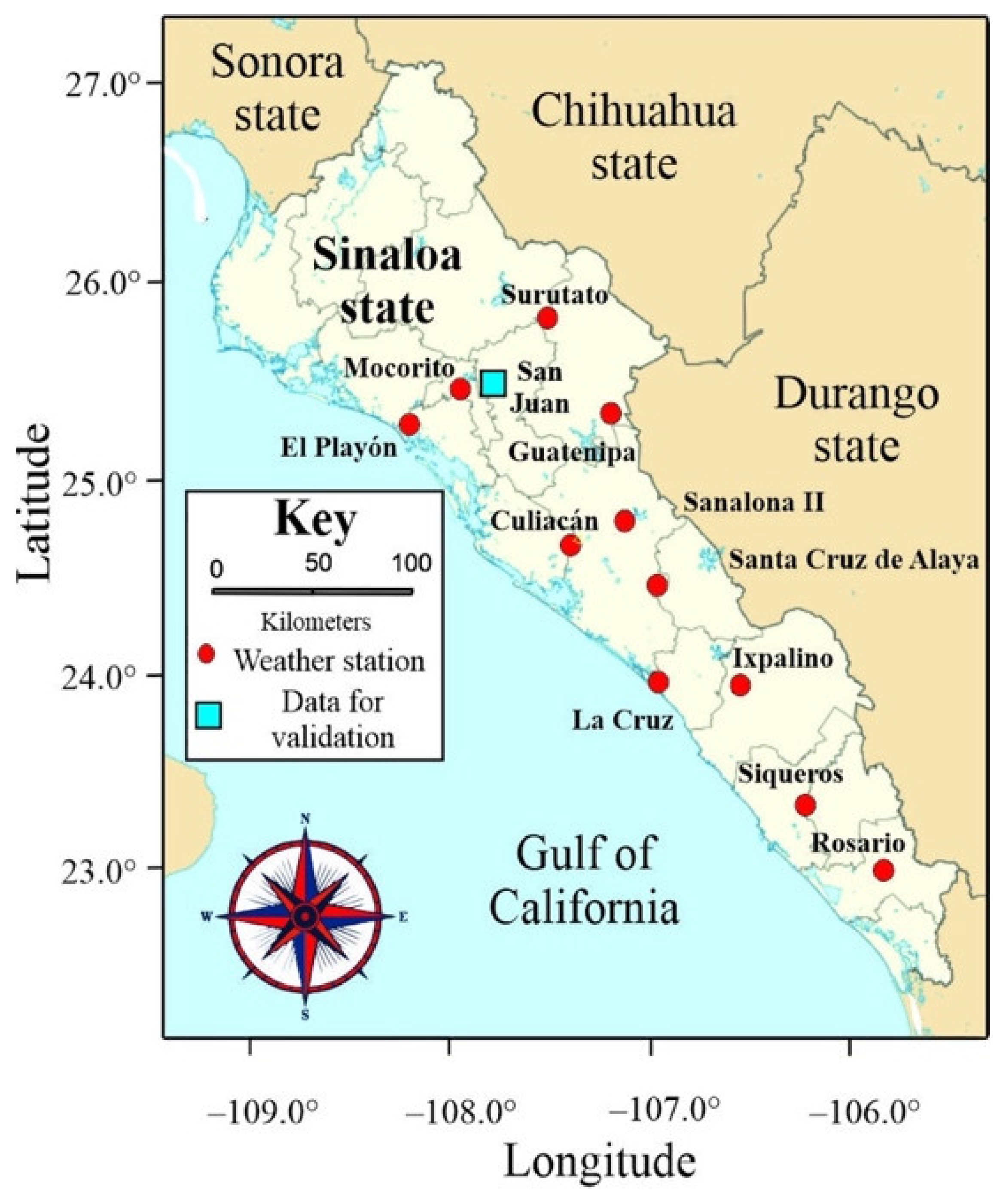
Figure 2.
Mean absolute error (MAE) and root mean square error (RMSE) of the average daily reference evapotranspiration between seven alternative methods () and the Penman–Monteith method with limited data (EToPM) (mm day–1).
Figure 2.
Mean absolute error (MAE) and root mean square error (RMSE) of the average daily reference evapotranspiration between seven alternative methods () and the Penman–Monteith method with limited data (EToPM) (mm day–1).
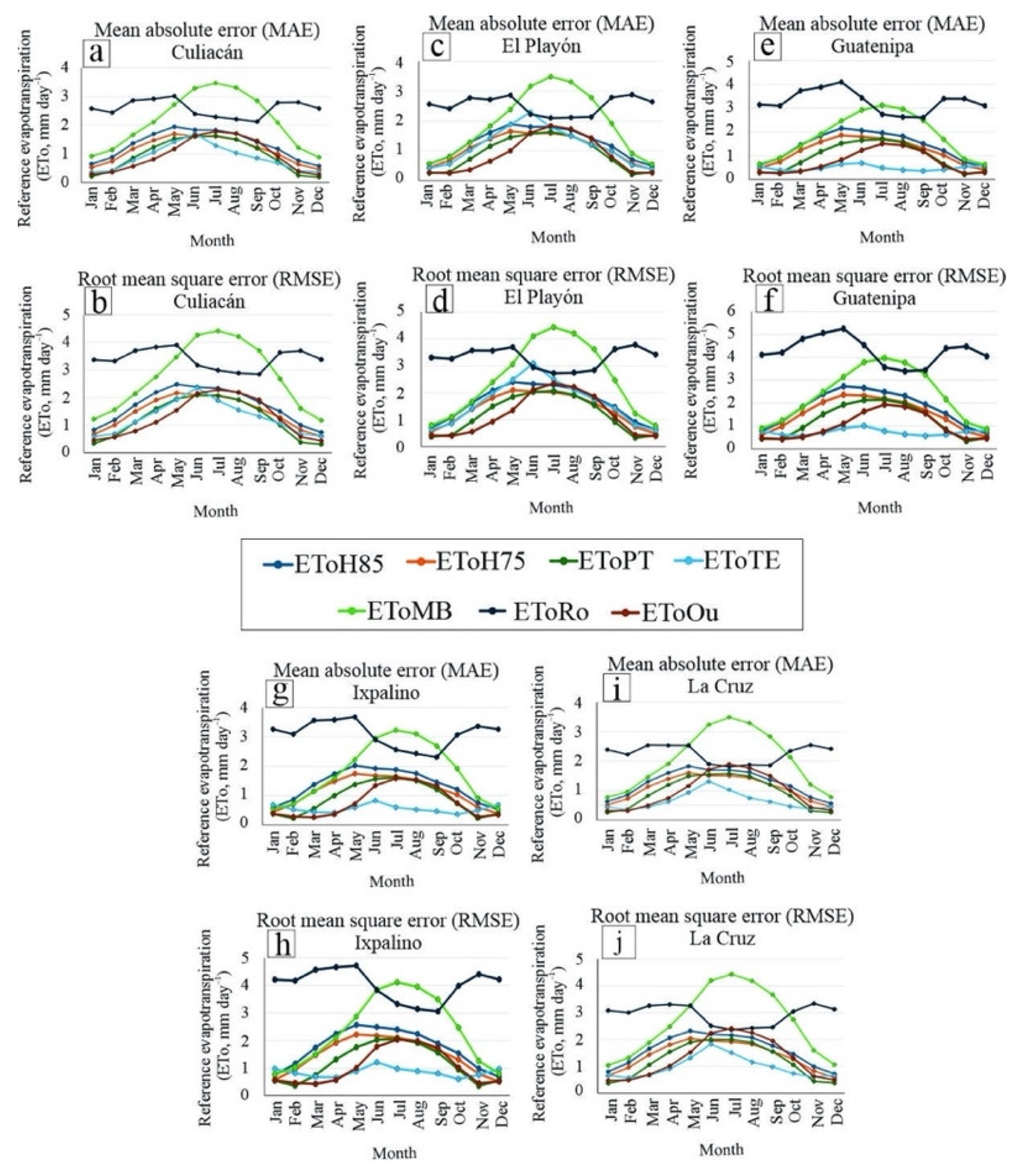
Figure 3.
Mean absolute error (MAE) and root mean square error (RMSE) of the average daily reference evapotranspiration between seven alternative methods () and the Penman–Monteith method with limited data (EToPM) (mm day–1; continuation).
Figure 3.
Mean absolute error (MAE) and root mean square error (RMSE) of the average daily reference evapotranspiration between seven alternative methods () and the Penman–Monteith method with limited data (EToPM) (mm day–1; continuation).
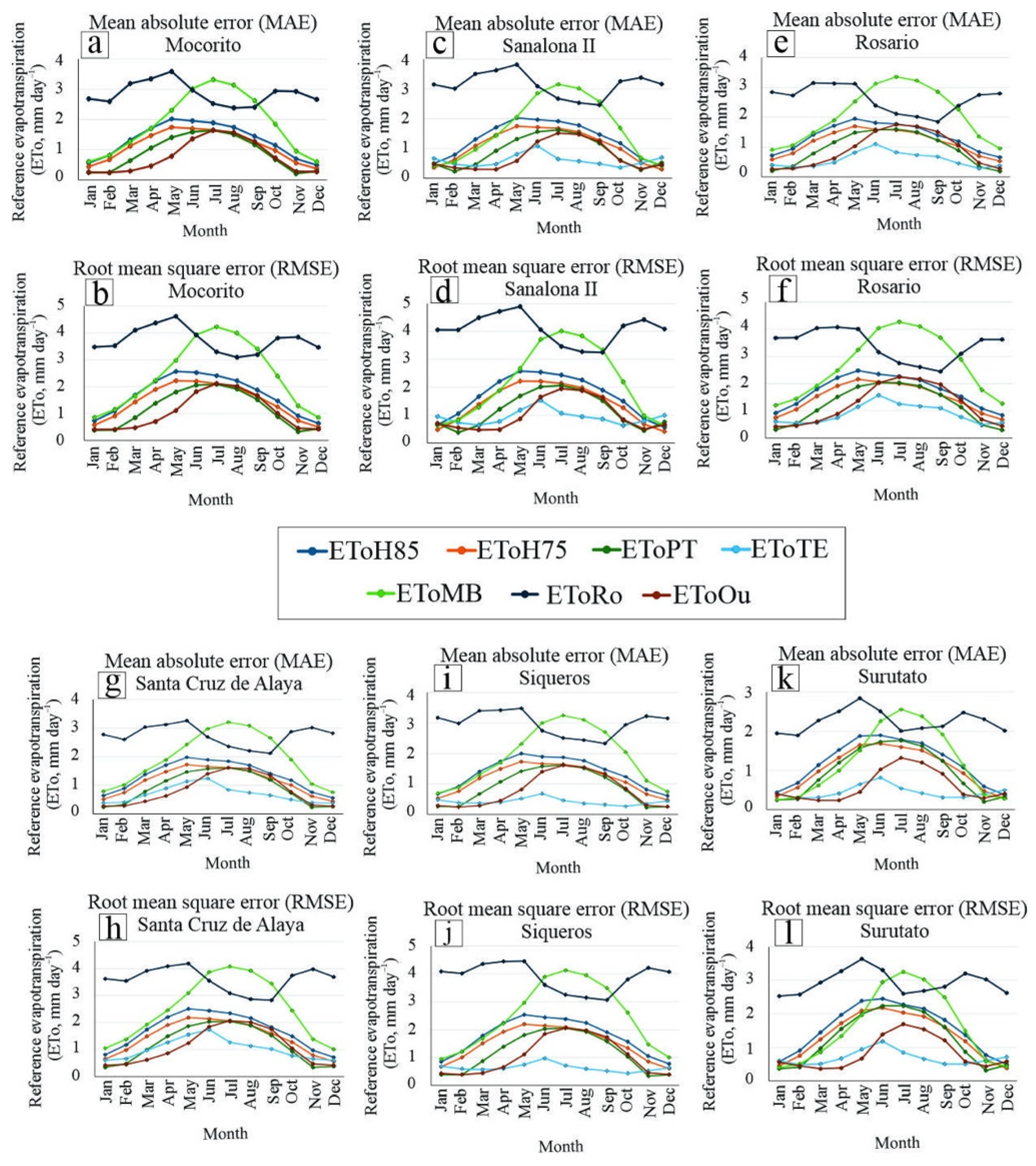
Figure 4.
Multiple linear and nonlinear regressions between Penman–Monteith annual cumulated reference evapotranspiration with limited data (EToPM) and with models (EToPMP).
Figure 4.
Multiple linear and nonlinear regressions between Penman–Monteith annual cumulated reference evapotranspiration with limited data (EToPM) and with models (EToPMP).
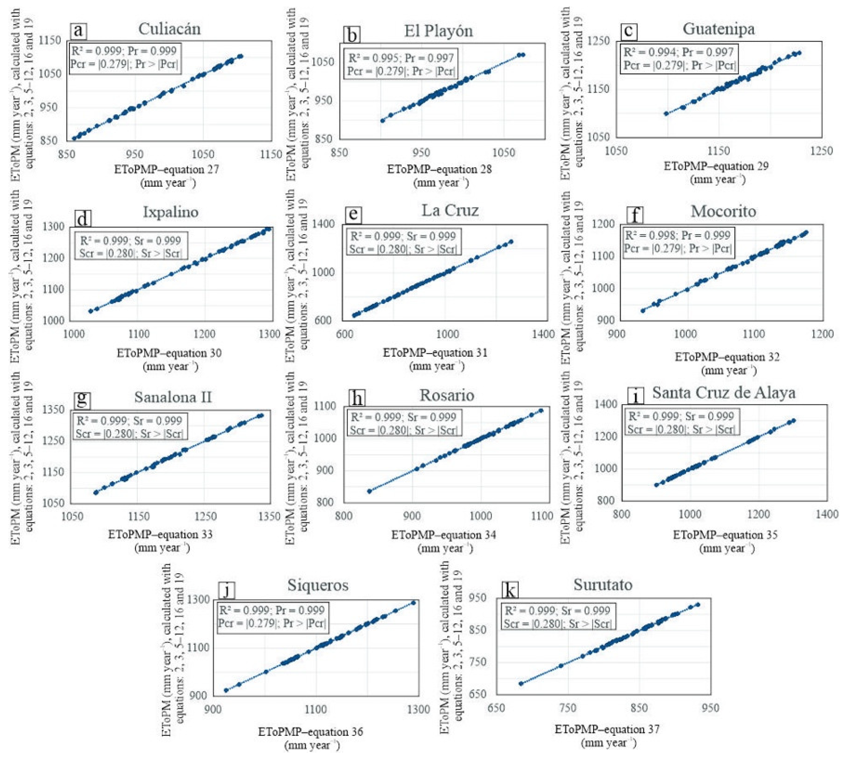
Figure 5.
Temporal variation of residuals generated between Penman–Monteith annual cumulated reference evapotranspiration with limited data (EToPM) and with models (EToPMP).
Figure 5.
Temporal variation of residuals generated between Penman–Monteith annual cumulated reference evapotranspiration with limited data (EToPM) and with models (EToPMP).
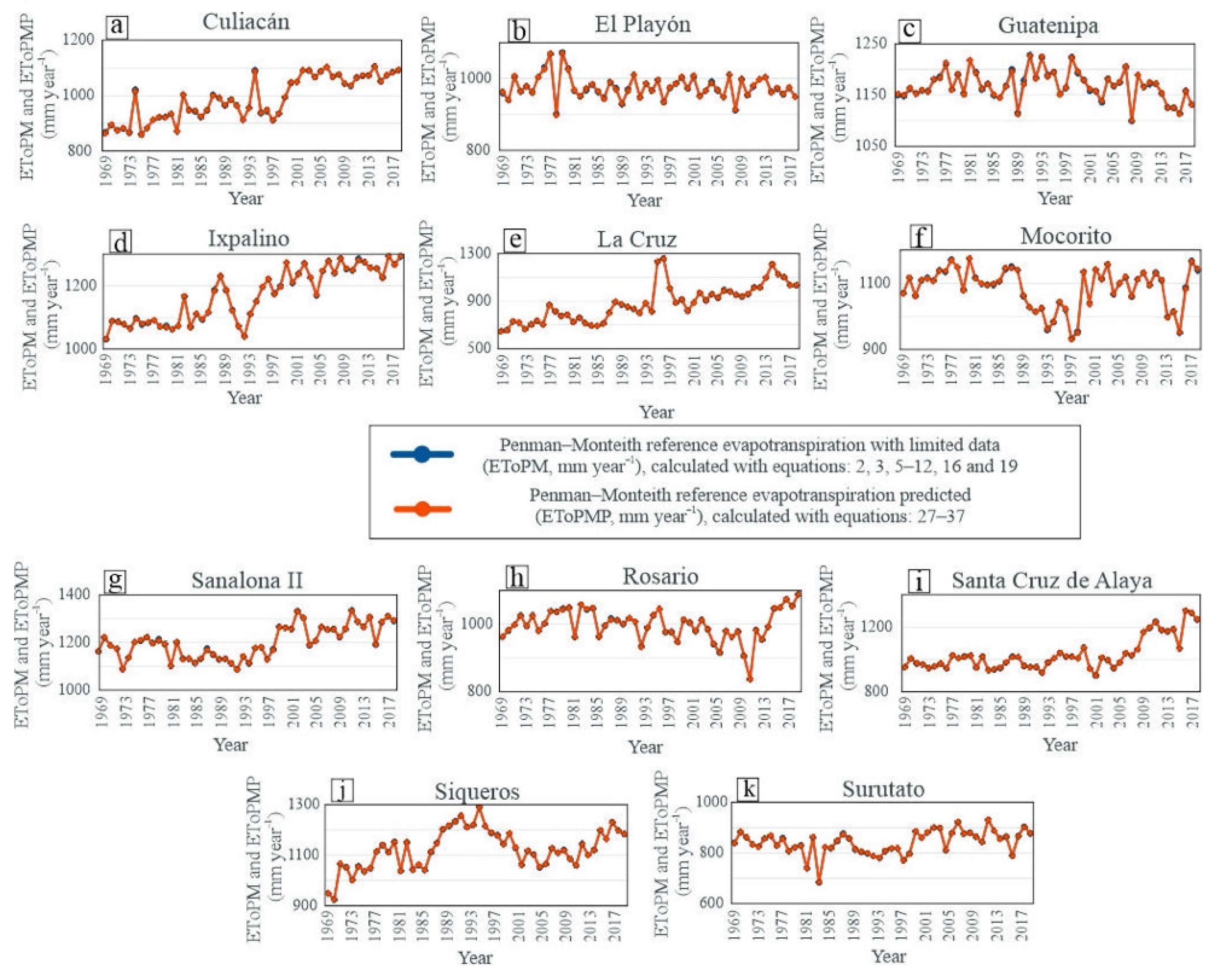
Figure 6.
Dispersion of daily Penman–Monteith reference evapotranspiration, with limited data in Mocorito (EToPM) and with observed data in San Juan (EToPMO) (mm day–1).
Figure 6.
Dispersion of daily Penman–Monteith reference evapotranspiration, with limited data in Mocorito (EToPM) and with observed data in San Juan (EToPMO) (mm day–1).
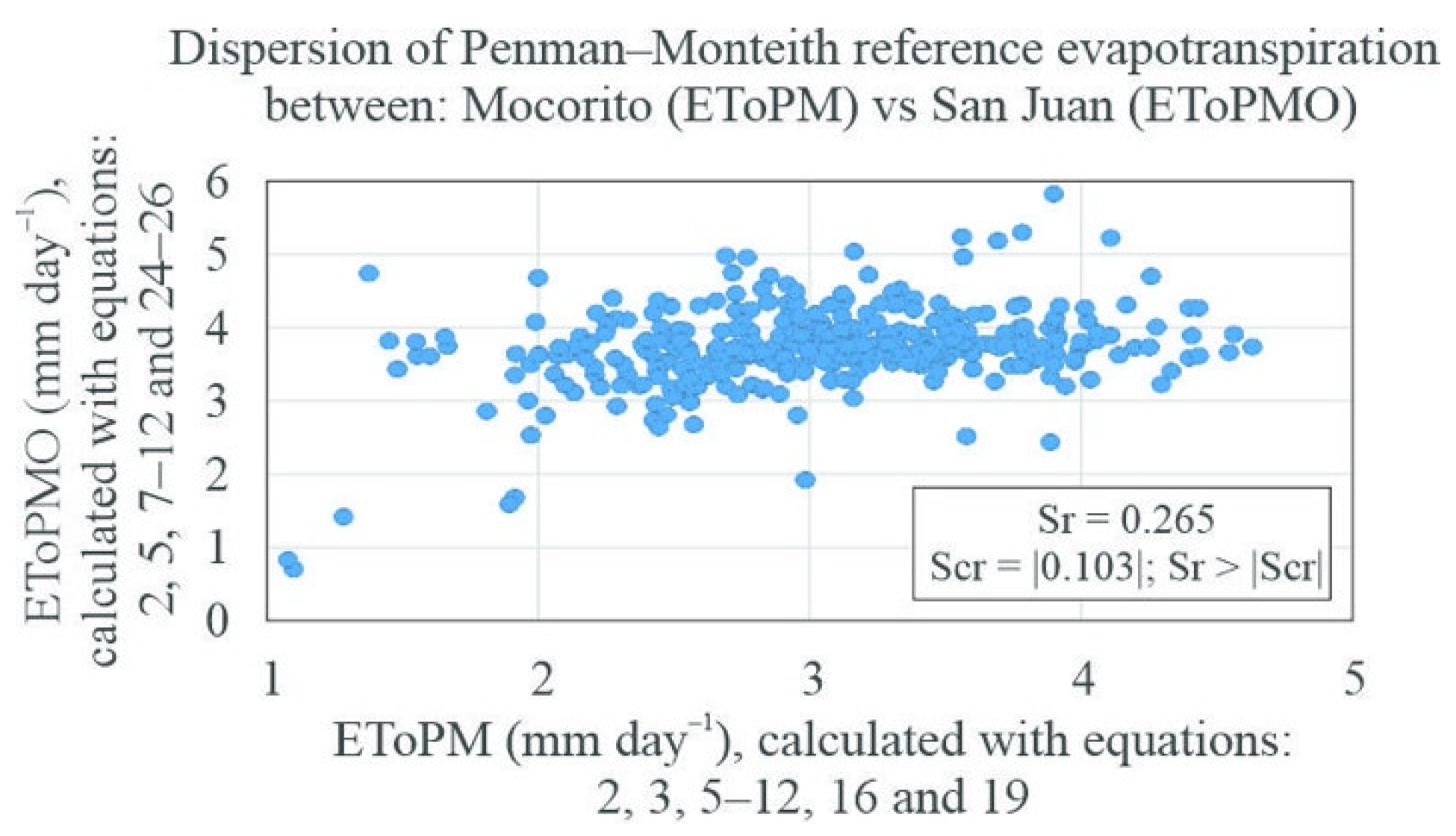

Table 1.
Maximum, minimum, and average daily values for Tmax, Tmin, Tmean (°C) and Eva (mm), for the period 1969–2018.
Table 1.
Maximum, minimum, and average daily values for Tmax, Tmin, Tmean (°C) and Eva (mm), for the period 1969–2018.
| Weather station | Statistical inference | Tmax (°C) | Tmin (°C) | Tmean (°C) | Eva (mm) |
| Culiacán | Average | 32.921 | 19.545 | 26.230 | 5.769 |
| maximum | 46.000 | 30.000 | 36.700 | 17.900 | |
| Minimum | 15.500 | 2.000 | 11.000 | 0.000 | |
| El Playón | Average | 31.361 | 16.863 | 24.112 | 6.648 |
| maximum | 45.500 | 37.000 | 38.000 | 17.800 | |
| Minimum | 13.000 | –6.000 | 8.750 | 0.100 | |
| Guatenipa | Average | 34.633 | 17.789 | 26.211 | 4.890 |
| maximum | 47.000 | 30.000 | 36.500 | 14.700 | |
| Minimum | 15.000 | 0.500 | 11.500 | 0.000 | |
| Ixpalino | Average | 34.229 | 17.318 | 25.774 | 4.878 |
| maximum | 46.000 | 28.500 | 34.250 | 17.400 | |
| Minimum | 18.000 | –1.200 | 11.400 | 0.100 | |
| La Cruz | Average | 30.299 | 17.447 | 23.872 | 4.409 |
| maximum | 42.000 | 33.000 | 34.500 | 18.000 | |
| Minimum | 12.000 | 0.000 | 9.100 | 0.000 | |
| Mocorito | Average | 32.971 | 17.318 | 25.144 | No value |
| maximum | 45.000 | 32.000 | 37.500 | No value | |
| Minimum | 9.000 | 0.000 | 6.250 | No value | |
| Sanalona II | Average | 33.872 | 15.847 | 24.860 | 5.464 |
| maximum | 44.000 | 28.500 | 35.000 | 17.800 | |
| Minimum | 17.000 | –5.000 | 8.250 | 0.000 | |
| Rosario | Average | 32.659 | 18.735 | 25.697 | 4.810 |
| maximum | 41.000 | 31.000 | 35.000 | 16.600 | |
| Minimum | 17.000 | 1.400 | 12.750 | 0.000 | |
| Santa Cruz de Alaya | Average | 32.476 | 17.763 | 25.118 | 5.543 |
| maximum | 43.000 | 34.000 | 37.000 | 15.400 | |
| Minimum | 13.400 | 1.000 | 11.800 | 0.000 | |
| Siqueros | Average | 33.907 | 17.958 | 25.932 | 4.746 |
| maximum | 43.000 | 28.500 | 34.500 | 14.600 | |
| Minimum | 17.000 | –0.500 | 11.000 | 0.000 | |
| Surutato | Average | 24.995 | 7.257 | 16.126 | 3.976 |
| maximum | 37.500 | 20.500 | 27.500 | 12.500 | |
| Minimum | 9.000 | –6.000 | 2.300 | 0.000 |
Table 2.
Average daily reference evapotranspiration (ETo) estimated using seven alternative methods () and the Penman–Monteith method with limited data (EToPM), for the period 1969–2018 (mm day–1).
Table 2.
Average daily reference evapotranspiration (ETo) estimated using seven alternative methods () and the Penman–Monteith method with limited data (EToPM), for the period 1969–2018 (mm day–1).
| Weather station | Average reference evapotranspiration (mm day–1) 1969–2018 (mm day–1) |
||||||||
| Month | EToPM | EToH85 | EToH75 | EToPT | EToTE | EToMB | EToRo | EToOu | |
| Culiacán | Jan | 2.196 | 3.245 | 3.047 | 2.317 | 2.190 | 3.668 | 6.363 | 2.494 |
| Feb | 2.467 | 4.040 | 3.794 | 3.180 | 2.895 | 4.491 | 6.792 | 3.054 | |
| Mar | 2.854 | 5.064 | 4.756 | 4.246 | 3.990 | 5.545 | 7.484 | 3.771 | |
| Apr | 3.219 | 6.031 | 5.664 | 5.264 | 4.935 | 6.719 | 8.088 | 4.569 | |
| May | 3.413 | 6.564 | 6.164 | 5.889 | 5.647 | 7.781 | 8.317 | 5.291 | |
| Jun | 3.078 | 6.108 | 5.736 | 5.717 | 5.835 | 8.501 | 7.085 | 5.781 | |
| Jul | 2.923 | 5.885 | 5.527 | 5.553 | 4.775 | 8.497 | 6.642 | 5.778 | |
| Aug | 2.724 | 5.483 | 5.149 | 5.156 | 4.224 | 8.063 | 6.298 | 5.483 | |
| Sep | 2.488 | 4.843 | 4.548 | 4.482 | 3.751 | 7.248 | 6.038 | 4.928 | |
| Oct | 2.601 | 4.497 | 4.223 | 3.843 | 3.529 | 5.975 | 7.097 | 4.063 | |
| Nov | 2.397 | 3.682 | 3.458 | 2.776 | 2.680 | 4.429 | 7.066 | 3.011 | |
| Dec | 2.112 | 3.047 | 2.861 | 2.109 | 1.996 | 3.537 | 6.283 | 2.405 | |
| El Playón | Jan | 2.298 | 3.199 | 3.004 | 2.094 | 2.614 | 3.197 | 6.428 | 2.174 |
| Feb | 2.553 | 3.981 | 3.739 | 2.957 | 3.304 | 3.946 | 6.819 | 2.683 | |
| Mar | 2.866 | 4.939 | 4.638 | 4.007 | 4.413 | 4.931 | 7.341 | 3.353 | |
| Apr | 3.070 | 5.747 | 5.397 | 4.961 | 5.425 | 6.088 | 7.593 | 4.140 | |
| May | 3.273 | 6.326 | 5.941 | 5.606 | 6.211 | 7.074 | 7.932 | 4.810 | |
| Jun | 2.847 | 5.813 | 5.460 | 5.429 | 6.554 | 8.021 | 6.564 | 5.454 | |
| Jul | 2.722 | 5.625 | 5.283 | 5.346 | 5.527 | 8.304 | 6.125 | 5.647 | |
| Aug | 2.621 | 5.349 | 5.023 | 5.060 | 4.979 | 7.943 | 6.027 | 5.402 | |
| Sep | 2.470 | 4.819 | 4.526 | 4.464 | 4.411 | 7.110 | 6.020 | 4.835 | |
| Oct | 2.585 | 4.440 | 4.170 | 3.736 | 4.142 | 5.664 | 7.075 | 3.851 | |
| Nov | 2.524 | 3.692 | 3.467 | 2.612 | 3.192 | 4.032 | 7.320 | 2.742 | |
| Dec | 2.263 | 3.053 | 2.867 | 1.920 | 2.483 | 3.131 | 6.523 | 2.129 | |
| Guatenipa | Jan | 2.596 | 3.578 | 3.360 | 2.331 | 1.785 | 3.618 | 7.677 | 2.460 |
| Feb | 2.999 | 4.589 | 4.309 | 3.379 | 2.476 | 4.584 | 8.479 | 3.117 | |
| Mar | 3.544 | 5.877 | 5.520 | 4.682 | 3.498 | 5.819 | 9.570 | 3.957 | |
| Apr | 4.040 | 7.102 | 6.670 | 5.971 | 4.530 | 7.200 | 10.506 | 4.896 | |
| May | 4.321 | 7.798 | 7.323 | 6.767 | 5.260 | 8.275 | 10.972 | 5.627 | |
| Jun | 3.906 | 7.299 | 6.855 | 6.604 | 4.891 | 8.710 | 9.640 | 5.923 | |
| Jul | 3.141 | 6.304 | 5.921 | 5.861 | 3.516 | 8.149 | 7.611 | 5.541 | |
| Aug | 2.898 | 5.834 | 5.479 | 5.417 | 3.050 | 7.680 | 7.144 | 5.223 | |
| Sep | 2.724 | 5.222 | 4.904 | 4.733 | 2.715 | 6.897 | 7.065 | 4.690 | |
| Oct | 2.955 | 4.898 | 4.600 | 3.986 | 2.527 | 5.661 | 8.442 | 3.850 | |
| Nov | 2.815 | 4.032 | 3.786 | 2.801 | 2.055 | 4.244 | 8.482 | 2.886 | |
| Dec | 2.462 | 3.316 | 3.115 | 2.096 | 1.599 | 3.451 | 7.460 | 2.346 | |
| Ixpalino | Jan | 2.906 | 3.859 | 3.624 | 2.449 | 1.862 | 3.721 | 8.171 | 2.530 |
| Feb | 3.257 | 4.787 | 4.495 | 3.418 | 2.445 | 4.526 | 8.739 | 3.077 | |
| Mar | 3.676 | 5.894 | 5.535 | 4.569 | 3.271 | 5.513 | 9.430 | 3.749 | |
| Apr | 3.993 | 6.876 | 6.458 | 5.653 | 4.062 | 6.629 | 9.966 | 4.508 | |
| May | 4.058 | 7.323 | 6.877 | 6.274 | 4.801 | 7.623 | 10.032 | 5.184 | |
| Jun | 3.479 | 6.648 | 6.243 | 6.047 | 4.715 | 8.354 | 8.329 | 5.681 | |
| Jul | 3.109 | 6.157 | 5.782 | 5.716 | 3.657 | 8.284 | 7.291 | 5.633 | |
| Aug | 2.855 | 5.690 | 5.344 | 5.289 | 3.160 | 7.862 | 6.775 | 5.346 | |
| Sep | 2.616 | 5.049 | 4.742 | 4.627 | 2.884 | 7.105 | 6.475 | 4.831 | |
| Oct | 2.842 | 4.794 | 4.502 | 4.013 | 2.767 | 5.938 | 7.803 | 4.038 | |
| Nov | 2.933 | 4.191 | 3.936 | 2.958 | 2.221 | 4.469 | 8.546 | 3.039 | |
| Dec | 2.755 | 3.609 | 3.389 | 2.252 | 1.715 | 3.631 | 8.015 | 2.469 | |
| La Cruz | Jan | 2.143 | 3.162 | 2.969 | 2.206 | 1.625 | 3.382 | 5.990 | 2.300 |
| Feb | 2.365 | 3.878 | 3.642 | 3.003 | 2.114 | 4.062 | 6.305 | 2.762 | |
| Mar | 2.624 | 4.732 | 4.444 | 3.956 | 2.93 | 4.987 | 6.715 | 3.391 | |
| Apr | 2.862 | 5.516 | 5.181 | 4.837 | 3.658 | 6.015 | 7.073 | 4.090 | |
| May | 2.909 | 5.863 | 5.506 | 5.318 | 4.264 | 7.001 | 7.019 | 4.761 | |
| Jun | 2.504 | 5.312 | 4.988 | 5.054 | 4.583 | 7.833 | 5.669 | 5.327 | |
| Jul | 2.415 | 5.154 | 4.840 | 4.951 | 3.884 | 7.996 | 5.358 | 5.437 | |
| Aug | 2.368 | 4.991 | 4.688 | 4.763 | 3.393 | 7.667 | 5.386 | 5.213 | |
| Sep | 2.221 | 4.50 | 4.226 | 4.224 | 3.036 | 6.949 | 5.307 | 4.726 | |
| Oct | 2.276 | 4.135 | 3.883 | 3.615 | 2.734 | 5.727 | 6.062 | 3.894 | |
| Nov | 2.252 | 3.539 | 3.324 | 2.695 | 2.089 | 4.258 | 6.490 | 2.895 | |
| Dec | 2.071 | 2.987 | 2.806 | 2.041 | 1.521 | 3.339 | 5.959 | 2.271 | |
Table 3.
Average daily reference evapotranspiration (ETo) estimated using seven alternative methods and the Penman–Monteith method with limited data (EToPM) for the period 1969–2018 (mm day–1; continuation).
Table 3.
Average daily reference evapotranspiration (ETo) estimated using seven alternative methods and the Penman–Monteith method with limited data (EToPM) for the period 1969–2018 (mm day–1; continuation).
| Weather station | Average reference evapotranspiration (mm day–1) 1969–2018 (mm day–1) |
||||||||
|---|---|---|---|---|---|---|---|---|---|
| Month | EToPM | EToH85 | EToH75 | EToPT | EToTE | EToMB | EToRo | EToOu | |
| Mocorito | Jan | 2.350 | 3.263 | 3.064 | 2.135 | No value value | 3.319 | 6.675 | 2.257 |
| Feb | 2.694 | 4.142 | 3.890 | 3.050 | No value | 4.137 | 7.285 | 2.813 | |
| Mar | 3.228 | 5.366 | 5.039 | 4.261 | No value | 5.261 | 8.366 | 3.577 | |
| Apr | 3.698 | 6.525 | 6.128 | 5.450 | No value | 6.509 | 9.258 | 4.426 | |
| May | 3.969 | 7.223 | 6.783 | 6.238 | No value | 7.69 | 9.756 | 5.229 | |
| Jun | 3.594 | 6.806 | 6.391 | 6.190 | No value | 8.553 | 8.551 | 5.816 | |
| Jul | 3.107 | 6.160 | 5.785 | 5.747 | No value | 8.422 | 7.213 | 5.727 | |
| Aug | 2.832 | 5.642 | 5.299 | 5.256 | No value | 7.888 | 6.673 | 5.364 | |
| Sep | 2.687 | 5.098 | 4.788 | 4.640 | No value | 7.066 | 6.705 | 4.805 | |
| Oct | 2.700 | 4.554 | 4.277 | 3.796 | No value | 5.685 | 7.440 | 3.866 | |
| Nov | 2.532 | 3.703 | 3.477 | 2.639 | No value | 4.123 | 7.407 | 2.804 | |
| Dec | 2.242 | 3.039 | 2.854 | 1.932 | No value | 3.214 | 6.537 | 2.186 | |
| Sanalona II | Jan | 2.925 | 3.728 | 3.501 | 2.246 | 1.928 | 3.417 | 7.996 | 2.323 |
| Feb | 3.273 | 4.665 | 4.381 | 3.233 | 2.598 | 4.219 | 8.590 | 2.869 | |
| Mar | 3.706 | 5.816 | 5.462 | 4.433 | 3.570 | 5.251 | 9.354 | 3.571 | |
| Apr | 4.103 | 6.934 | 6.512 | 5.622 | 4.542 | 6.455 | 10.136 | 4.389 | |
| May | 4.221 | 7.494 | 7.038 | 6.338 | 5.396 | 7.530 | 10.390 | 5.120 | |
| Jun | 3.64 | 6.872 | 6.453 | 6.185 | 5.339 | 8.329 | 8.786 | 5.663 | |
| Jul | 3.187 | 6.279 | 5.897 | 5.794 | 4.027 | 8.234 | 7.534 | 5.599 | |
| Aug | 2.925 | 5.790 | 5.437 | 5.345 | 3.629 | 7.790 | 7.011 | 5.297 | |
| Sep | 2.711 | 5.156 | 4.842 | 4.667 | 3.233 | 6.998 | 6.810 | 4.759 | |
| Oct | 2.967 | 4.863 | 4.567 | 3.942 | 2.945 | 5.686 | 8.210 | 3.866 | |
| Nov | 3.022 | 4.136 | 3.884 | 2.755 | 2.298 | 4.144 | 8.654 | 2.818 | |
| Dec | 2.796 | 3.49 | 3.277 | 2.034 | 1.767 | 3.312 | 7.892 | 2.252 | |
| Rosario | Jan | 2.442 | 3.601 | 3.382 | 2.546 | 1.924 | 3.904 | 7.030 | 2.655 |
| Feb | 2.796 | 4.468 | 4.196 | 3.421 | 2.439 | 4.669 | 7.635 | 3.175 | |
| Mar | 3.181 | 5.467 | 5.134 | 4.451 | 3.328 | 5.577 | 8.267 | 3.793 | |
| Apr | 3.465 | 6.320 | 5.935 | 5.391 | 4.058 | 6.602 | 8.687 | 4.490 | |
| May | 3.469 | 6.617 | 6.214 | 5.867 | 4.685 | 7.534 | 8.516 | 5.123 | |
| Jun | 2.987 | 5.978 | 5.614 | 5.566 | 4.676 | 8.137 | 6.973 | 5.533 | |
| Jul | 2.695 | 5.575 | 5.236 | 5.276 | 3.864 | 8.075 | 6.159 | 5.491 | |
| Aug | 2.497 | 5.200 | 4.884 | 4.927 | 3.525 | 7.703 | 5.755 | 5.238 | |
| Sep | 2.235 | 4.559 | 4.282 | 4.287 | 3.199 | 7.000 | 5.322 | 4.760 | |
| Oct | 2.339 | 4.273 | 4.013 | 3.776 | 2.870 | 5.991 | 6.189 | 4.074 | |
| Nov | 2.412 | 3.812 | 3.580 | 2.968 | 2.308 | 4.659 | 6.998 | 3.168 | |
| Dec | 2.300 | 3.362 | 3.157 | 2.372 | 1.816 | 3.847 | 6.809 | 2.616 | |
| Santa Cruz de Alaya | Jan | 2.374 | 3.403 | 3.196 | 2.329 | 2.394 | 3.645 | 6.847 | 2.479 |
| Feb | 2.638 | 4.205 | 3.949 | 3.201 | 3.031 | 4.433 | 7.239 | 3.014 | |
| Mar | 3.034 | 5.246 | 4.926 | 4.285 | 3.932 | 5.452 | 7.932 | 3.707 | |
| Apr | 3.425 | 6.253 | 5.872 | 5.335 | 4.789 | 6.551 | 8.615 | 4.455 | |
| May | 3.600 | 6.787 | 6.374 | 5.963 | 5.366 | 7.492 | 8.869 | 5.095 | |
| Jun | 3.242 | 6.35 | 5.963 | 5.819 | 5.185 | 8.146 | 7.714 | 5.539 | |
| Jul | 2.886 | 5.861 | 5.504 | 5.472 | 4.073 | 8.021 | 6.733 | 5.454 | |
| Aug | 2.619 | 5.367 | 5.040 | 5.024 | 3.634 | 7.587 | 6.170 | 5.159 | |
| Sep | 2.413 | 4.762 | 4.472 | 4.384 | 3.296 | 6.843 | 5.944 | 4.653 | |
| Oct | 2.660 | 4.555 | 4.278 | 3.825 | 3.205 | 5.732 | 7.295 | 3.898 | |
| Nov | 2.603 | 3.859 | 3.624 | 2.806 | 2.801 | 4.339 | 7.629 | 2.950 | |
| Dec | 2.324 | 3.229 | 3.032 | 2.144 | 2.259 | 3.537 | 6.874 | 2.405 | |
| Siqueros | Jan | 2.752 | 3.828 | 3.595 | 2.557 | 2.056 | 3.870 | 7.867 | 2.632 |
| Feb | 3.081 | 4.703 | 4.417 | 3.470 | 2.513 | 4.637 | 8.365 | 3.153 | |
| Mar | 3.463 | 5.728 | 5.380 | 4.541 | 3.232 | 5.557 | 8.950 | 3.779 | |
| Apr | 3.795 | 6.672 | 6.265 | 5.557 | 3.887 | 6.597 | 9.490 | 4.486 | |
| May | 3.829 | 7.048 | 6.619 | 6.108 | 4.450 | 7.531 | 9.462 | 5.121 | |
| Jun | 3.307 | 6.424 | 6.033 | 5.891 | 4.353 | 8.263 | 7.876 | 5.619 | |
| Jul | 3.044 | 6.066 | 5.697 | 5.649 | 3.500 | 8.243 | 7.124 | 5.605 | |
| Aug | 2.863 | 5.707 | 5.359 | 5.305 | 3.093 | 7.868 | 6.794 | 5.351 | |
| Sep | 2.631 | 5.087 | 4.777 | 4.664 | 2.883 | 7.131 | 6.504 | 4.849 | |
| Oct | 2.750 | 4.739 | 4.451 | 4.040 | 2.749 | 6.042 | 7.496 | 4.109 | |
| Nov | 2.788 | 4.143 | 3.890 | 3.053 | 2.313 | 4.632 | 8.163 | 3.150 | |
| Dec | 2.601 | 3.579 | 3.362 | 2.373 | 1.953 | 3.795 | 7.681 | 2.581 | |
| Surutato | Jan | 1.941 | 2.651 | 2.490 | 1.750 | 1.356 | 2.086 | 5.081 | 1.418 |
| Feb | 2.177 | 3.376 | 3.171 | 2.614 | 1.883 | 2.669 | 5.529 | 1.815 | |
| Mar | 2.472 | 4.303 | 4.041 | 3.688 | 2.613 | 3.462 | 6.137 | 2.354 | |
| Apr | 2.85 | 5.372 | 5.045 | 4.828 | 3.342 | 4.485 | 7.018 | 3.050 | |
| May | 3.035 | 6.066 | 5.697 | 5.565 | 3.982 | 5.471 | 7.620 | 3.721 | |
| Jun | 2.640 | 5.753 | 5.403 | 5.471 | 3.866 | 6.345 | 6.803 | 4.315 | |
| Jul | 2.137 | 5.022 | 4.716 | 4.972 | 2.802 | 6.227 | 5.403 | 4.234 | |
| Aug | 2.103 | 4.83 | 4.536 | 4.716 | 2.569 | 5.938 | 5.455 | 4.038 | |
| Sep | 2.050 | 4.392 | 4.125 | 4.113 | 2.269 | 5.246 | 5.587 | 3.567 | |
| Oct | 2.168 | 3.899 | 3.661 | 3.238 | 2.107 | 3.982 | 6.162 | 2.708 | |
| Nov | 2.149 | 3.131 | 2.940 | 2.151 | 1.610 | 2.722 | 5.992 | 1.851 | |
| Dec | 1.929 | 2.533 | 2.379 | 1.553 | 1.217 | 2.049 | 5.179 | 1.393 | |
Table 4.
Normality of residuals (dimensionless).
| Weather station | Shapiro–Wilk (W) | P(normal) |
|---|---|---|
| Culiacán | 0.969 | 0.207 |
| EL Playón | 0.976 | 0.411 |
| Guatenipa | 0.975 | 0.371 |
| Ixpalino | 0.891 | 0.001 |
| La Cruz | 0.905 | 0.001 |
| Mocorito | 0.983 | 0.662 |
| Sanalona II | 0.903 | 0.001 |
| Rosario | 0.940 | 0.013 |
| Santa Cruz de Alaya | 0.940 | 0.013 |
| Siqueros | 0.981 | 0.593 |
| Surutato | 0.952 | 0.042 |
Disclaimer/Publisher’s Note: The statements, opinions and data contained in all publications are solely those of the individual author(s) and contributor(s) and not of MDPI and/or the editor(s). MDPI and/or the editor(s) disclaim responsibility for any injury to people or property resulting from any ideas, methods, instructions or products referred to in the content. |
© 2024 by the authors. Licensee MDPI, Basel, Switzerland. This article is an open access article distributed under the terms and conditions of the Creative Commons Attribution (CC BY) license (http://creativecommons.org/licenses/by/4.0/).
Copyright: This open access article is published under a Creative Commons CC BY 4.0 license, which permit the free download, distribution, and reuse, provided that the author and preprint are cited in any reuse.


