
Submitted:
20 November 2024
Posted:
22 November 2024
Read the latest preprint version here
Abstract
We examine the feasibility of non-invasive cancer detection using the X-ray scattering properties of nails in the canine model. 945 samples taken from 266 dogs were measured, with 84 animals diagnosed with cancer. To analyze the obtained X-ray diffraction patterns of keratin, we propose a method based on the two-dimensional Fourier transformation of the images. We compare 350 combinations of data preprocessing steps and machine learning classifiers and determine corresponding performance metrics. Excellent classification results are demonstrated, with sensitivity or specificity achieving 100% and the best value for balanced accuracy being 87.5%. Our approach can be extended to human samples to develop a non-invasive, convenient, and cheap method for early cancer detection.
Keywords:
X-ray diffraction
; vitacrystallography
; cancer detection
; canine model
; keratin
; machine learning
; Fourier transformation
; ROC curves
; Principal Component Analysis
1. Introduction
Since its discovery [1,2], X-ray diffraction (XRD) has been a major tool in crystallography, uncovering the atom arrangements in crystalline solids. Diffraction patterns not only determine the symmetry of the crystal lattice but also reveal the electronic density at the lattice points, allowing the structure to be solved. The feasibility of enzyme crystallization [3] creates the pathway for biocrystallography. XRD on crystallized biological molecules deciphered the molecular content of complex structures; see [4] for historical overviews. Recently, it was shown that the X-ray scattering approach can be applied directly to biological tissues. This field of science, which we have called vitacrystallography [5], studies periodic structures in the extracellular matrix and their modifications induced by various diseases, especially cancer. Such modifications are detectable [5,6,7,8,9,10] and can lead to effective early cancer diagnostics. While most of the reports of cancer-induced changes are based on the alterations of X-ray scattering on lipids, the possibility of cancer detection using the keratin molecules of hair and nails was also discussed. Modifications associated with cancer in human hair were reported [11,12], but these measurements and their interpretations were disputed [13,14]. However, recent experiments [15] exhibited a high probability of cancer detection in dogs by the XRD patterns of their claws.
Studies of canine cancer are essential for two reasons. First, canines are excellent models since they spontaneously develop the same types of cancer as humans, leading to their use in comparative and translational oncology [16,17,18]. Second, 6 million pet dogs are estimated to be diagnosed with cancer in the United States [19], which puts an enormous burden on the animals and their owners. Early cancer detection is paramount for saving the lives of pets, and, at the same time, achievements in the canine model can be used to improve the treatment of human diseases. Comprehensive data can be collected from millions of dogs that visit the veterinary clinic each year, dramatically accelerating the development of new precision therapy that will benefit both dogs and their owners [19].
The potentially collected datasets require novel data representation and data analytics methods, including machine learning and artificial intelligence. Usually, for the XRD studies of biological tissue, the azimuthal integration is performed in the obtained two-dimensional (2D) image, and the data are represented in the intensity dependence on the momentum transfer q. This quantity corresponds to the scattering angle 2θ as q = (4π sin θ)/λ, where λ is the X-ray wavelength. This approach allows transparent physical interpretation of results because the momentum transfer is directly related to the periodicity d of molecular systems as q = 2π/d. In particular, XRD-based cancer detection [5,6,7,8,9,10] is related to specific features at 1.5 and 13.9 nm−1, linked to the packing of triglycerides and inter-fatty-acid molecular distances, respectively [20]. However, a significant amount of information will be lost after the azimuthal integration for materials with angular anisotropy, such as keratin.
In this work, we propose a method based on the 2D Fourier transformation of the XRD images and compare it to the previously developed 1D Fourier transformation approach [15]. We apply it to the dataset of 266 patients (dogs), with 104 of them diagnosed with cancer. As each dog provides more than one sample (cut from the claw), we have 945 XRD patterns, which we separated into the training (775 images) and test sets. We employ various data preprocessing steps, both standard and custom-developed, including Principal Component Analysis (PCA). Three machine learning algorithms are used to determine the performance metrics: Logistic Regression, Random Forest, and XGBoost. The first two classifiers are taken from the scikit-learn library [21], while the third comes from the XGBoost library [22]. We obtain and compare the classification metrics for 350 combinations of the preprocessing steps and classifiers. These metrics are further improved if we group the samples from the same patient. For several combinations, either sensitivity or specificity reaches 1, and the balanced accuracy can be up to 0.875.
2. Materials and Methods
2.1. Sample Preparation
Samples from 266 patients (dogs) were collected, with 104 of them diagnosed with cancer. The patients are either client-owned animals of various breeds or beagles from a laboratory colony. The ages of the dogs ranged from 0.5 to 17 years. Patients provided several samples each (four for most), prepared and measured independently. The final dataset had 945 samples.
The sample is a thin slice of hard outer shell tissue cut or shaved from the nail’s surface. They are produced by a surgical knife to cut a very thin surface layer of the nail’s outer hard shell with between 100 to 200 microns in thickness and an area of about 3 by 3 mm, as shown in Figure 1. It was shown previously that there was no visible difference between the samples obtained from dogs with and without cancer [15]. The samples were then placed into the specially designed holder, intended to hold the nail shaving under the X-ray beam, but no part of the sample holder would interact with the beam.
2.2. Diffraction Measurements
The custom-developed desktop X-ray diffractometer contains the beam delivery system, the sample receptacle, and the X-ray detector. We use the Xenocs X-ray source, a Genix 3D Cu with Fox 12–53 Cu Mirror, with a wavelength λ = 0.1540562 nm or energy of 8.04 keV. Xenocs also produced the focusing optics. The sample holder is placed on the receptacle, which includes a circular aperture beam collimator. The two-dimensional detector is an Advacam MiniPix SN1442 Si 500 µm with a 256-by-256-pixel array and a 55-by-55-micron pixel size. More details about our diffractometer can be found in Ref. [15]. The sample-to-detector distance for all samples was 20 mm, and the exposure time was 2 min. The samples were measured batch by batch; all results were obtained under the same experimental conditions. The experimental data were stored as 256-by-256 matrices of integers representing the photon counts. Each batch was complemented by at least one calibration file with silver behenate (AgBH) XRD patterns.
2.3. Data Analysis
2.3.1. Image Preprocessing
The raw XRD data were 2D images (256 × 256 pixels). Before further analysis, all images were preprocessed using the following steps:
- Raw data was calibrated using silver behenate (AgBH) to unify scales for different batches. The image was rescaled during calibration to adjust the q-range to the same value. The calibrated image is shown in Figure 2a.
- The images were centered and rotated to unify the positions of essential features. The data were also cropped to a circular shape to make them symmetric.
- Hot spots and hot pixels were removed, substituting them with the average intensity value over the circle with a certain radius.
- The intensity of the diffracted beam was normalized, i.e., the total intensity of the preprocessed images was adjusted to 5 mln counts. The final preprocessed image is shown in Figure 2b.
2.3.2. One-Dimensional Fourier Transformation
The azimuthal integration of the two-dimensional dataset is performed to obtain the one-dimensional curve for subsequent determination of Fourier coefficients. We use two types of integration: (i) integration over 360 degrees (AI) and (ii) separate integrations over each of the four sectors (AIS) shown in Figure 2b. These sectors contain either an arc or a peak, corresponding to the pitch of chiral keratin molecules or the intermolecular distance in molecular packing [23]. For the obtained dependencies of the intensity to the distance to the center, the regions close to the primary beam are cut, and the slope of the curve is removed for better Fourier series convergence (SR). One-dimensional Fourier coefficients are obtained via the Standard Discrete Fourier Transformation implemented in SciPy and NumPy libraries (1DF) or the custom procedure described in Ref. [15] (1DFC). We used Low Pass Fourier Filtration (LPF) to select only the most prominent low-frequency coefficients. Specifically, 30 coefficients were taken for AI curves or each of the four AIS curves.
2.3.3. Two-Dimensional Fourier Transformation
The two-dimensional (2D) Standard Discrete Fourier Transformation calculated the 2D Fourier coefficients (2DF). We used either the complete set (256 by 256 matrix) or 1257 complex Fourier coefficients obtained by the Low Pass Fourier Filtration with the 20th order cutoff. We tested different combinations of the Fourier coefficient components: real parts (Re), imaginary parts (Im), both real and imaginary parts (Re_Im), and the amplitudes (Am).
2.3.4. Additional Data Preprocessing Steps
Several optional steps can be taken for the data preprocessing. We can use the Standard Scaling procedure from the scikit-learn library [21] (STD) to standardize the contribution of features to the analysis and perform the Principal Component Analysis to reduce the number of variables. We exploit the following numbers of principal components: 3 (PCA_3), 50 (PCA_50), 100 (PCA_100), and 750 (PCA_750).
Another optional step is the removal of the primary beam. It can be removed from the original images before the Fourier transformations (BR) or in the reciprocal space (BRF). For the latter, we introduced the following procedure. The auxiliary matrices are constructed with zeroes everywhere except the locations of the bright circles at the center. 2D Fourier transformations of these matrices contain the Fourier coefficients of the primary beam images. The differences between Fourier coefficients of original and auxiliary matrices are the coefficients of the beam-less XRD signal.
The next step for all tasks is the preparation of the matrices for the machine-learning classifiers. These matrices have the dimensionality MxN, where M is the number of elements and N is the number of samples in the training set. For 2D cases where the Fourier coefficients are the matrices themselves, they are flattened, i.e., all the matrix elements are converted in a single row. In our studies, N = 775, while M changes from 30 for 1DF to 131,072 for Re_Im of the complete set of 2D Fourier coefficients.
2.3.5. Machine-Learning Classifiers
3. Results
The measured XRD patterns were randomly separated into the training and testing datasets. The training dataset contains 132 non-cancerous and 84 cancerous patients (775 samples). The testing dataset has 30 non-cancerous and 20 cancerous patients. Both training and testing data were preprocessed using the same procedure. The training dataset optimized the model, and then the testing dataset was classified by the optimized estimator. The modeling process was implemented as a pipeline, where different preprocessing steps and classifiers were called in various combinations to determine the best algorithm for diagnostics.
We used sensitivity (Sen_S), specificity (Spec_S), and balanced accuracy (BA_S) as performance metrics. Sensitivity is the proportion of the cancerous samples that were correctly identified. Similarly, specificity measures the proportion of non-cancerous samples that were correctly identified. Balanced accuracy = (specificity + sensitivity)/2. We also determine the receiver operating characteristics (ROC) curve and use the area under the ROC curve (AUC_S) as a metric. The results from the samples belonging to the same patient were averaged, and all performance metrics (Sen_P, Spec_P, BA_P, and AUC_P) were also calculated for the patients.
The best (in terms of BA_P) 10 combinations of the preprocessing steps and classifiers are shown in Table 1, with the nomenclature taken from Section 2. The best results from the other approaches are presented in Table 2. The first column provides the total ranking.
One can see from these tables that the best diagnosis is achieved by the Random Forest model based on imaginary parts of low-pass-filtered 2D Fourier coefficients with standard scaling and 100 principal components. The primary beam was removed in the reciprocal space. The proposed approach allows us to impose additional conditions on the search. Table 3 and Table 4 show the best results with the conditions of specificity or sensitivity greater than 0.9.
The comparison of the ROC curves can provide additional information. We present four characteristic curves for patients in Figure 3.
In Figure 3a, we present the red ROC curve for the best-performing combination of the data preprocessing steps and machine learning algorithms: Random Forest model based on imaginary parts of low-pass-filtered 2D Fourier coefficients with standard scaling, 100 principal components, and the primary beam removed in the reciprocal space. Almost the same combination but without standard scaling and principal components produces the blue ROC curve of this figure, with much worse metrics. Figure 3b compares the results of two different classifiers for the amplitudes of the complete set of 2D Fourier coefficients without beam removal, standard scaling, and principal component analysis. The Logistic Regression (in blue) produces a larger AUC than the Random Forest (in red). The balanced accuracy for LOG is also larger (0.84 vs. 0.78), although the results are the opposite for the specificity (0.93 vs. 0.97). It should be noted that this is the only case where the results of the Logistic Regression are comparable to those of two other classifiers. Usually, they are much worse.
Another type of visualization is representing data in the space of principal components. We use it in Figure 4 to compare two approaches to primary beam elimination. This figure shows the data corresponding to the amplitudes of low-pass-filtered 2D Fourier coefficients after the standard scaling, but for Figure 4a, the beam was removed in the reciprocal space, while for Figure 4b, it was done in the real space.
In both figures, there is a well-pronounced cluster of cancerous samples. However, in Figure 4a, the points outside this cluster also exhibit a separation. It manifests itself in the metrics. XGBoost provides the AUC of 0.82 and the BA of 0.78 for BRF, while these values are 0.75 and 0.7 for BR.
4. Discussion
Comparing the results obtained by different data preprocessing steps and machine-learning algorithms, we can reveal general trends and make several conclusions:
- Data representations based on 2D Fourier transformation are vastly superior to their 1D counterparts. It was expected because azimuthal integration eliminates anisotropy and leads to the loss of information for anisotropic structures, such as keratin.
- Random Forest and XGBoost outperform the Logistic Regression.
- Reducing the number of Fourier coefficients using the Low Pass Filter improves the diagnostics. Elimination of unimportant features provides a better focus for machine learning algorithms.
- Removing the area near the primary beam leads to better results. Our custom-developed approach to removing it in the reciprocal space works better than direct removal in the real space. However, sometimes the results are almost identical; see lines 8 and 9 of Table 1.
- Principal Component Analysis improves the results only with a proper choice of the number of principal components involved. If this number is too small (n=3) or too large (n=750), the diagnostics are worse than when n = 50 or 100.
- All the metrics for patients are much better than those for the samples. This can be expected because averaging the samples belonging to the same patient eliminates the outliers.
- For the 1D approach, our custom procedure [15] works better than the standard one.
5. Conclusions
In this paper, we have shown that the data analysis approaches based on Fourier coefficients are beneficial for analyzing anisotropic XRD patterns, especially with 2D transformation. We obtained excellent performance metrics, as for several combinations of the data preprocessing steps and machine learning algorithms, the sensitivity or specificity can reach 1. The best results are achieved by the Random Forest model based on imaginary parts of low-pass-filtered 2D Fourier coefficients with standard scaling, 100 principal components, and the primary beam removed in the reciprocal space. Our methods can be used for canine cancer detection based on the X-ray scans of dog’s nails and, in the future, extended to human cancer diagnostics.
Author Contributions
Conceptualization, L.M. and P.L.; methodology, A.A., O.A., S.M., A.L., D.L., and P.L.; software, A.A., O.A., and S.M.; validation, A.A., O.A., L.M., and P.L.; formal analysis, A.A.; investigation, A.A., O.A., S.M., D.Y., A.L., and D.L.; resources, D.Y. and D.L.; data curation, A.A.; writing—original draft preparation, A.A. and L.M.; writing—review and editing, L.M.; visualization, A.A. and S.M.; supervision, P.L.; project administration, D.Y. and P.L.; funding acquisition, D.Y. and P.L. All authors have read and agreed to the published version of the manuscript.
Funding
This research received no external funding.
Data Availability Statement
The files with the XRD patterns for the training and test datasets, as well as the complete table with a set of metrics obtained from different approaches, are available at Fourier-transformation-based analysis of X-ray diffraction pattern of keratin for cancer detection. The codes are available upon request.
Acknowledgments
We would like to thank the following clinics for providing the samples: Alternative Veterinary Therapies (NY), Animal Medical Center of Seattle (WA), Blue Pearl Veterinary Partners (PA), Bridge Animal Referral Center (WA), Burroughs Veterinary Services (OH), Ethos-WVRC (WI), Evans Family Pet Care (MN), Intervivo Solutions (ON, Canada), Lakeville Family Pet Clinic (MN), Maryville Small Animal Medical Center (TN), Ocean State Veterinary Specialists (RI), Sen Beevers (CA), Private Veterinary Specialties (NJ), Sage Centers - Campbell & SF (CA), Slaton Animal Hospital (TX), Spay Neuter Veterinary Clinic (NC), Summit Veterinary Referral Center (WA), VCA Sacramento (CA), and Veterinary Specialty Center (IL).
Conflicts of Interest
P.L. is a shareholder of Matur UK, Ltd and Arion Diagnostics, Inc. D.Y. and D.L. are shareholders of Arion Diagnostics, Inc. A.A., O.A., and S.M. are consultants for Matur UK, Ltd. A.L. and L.M. are consultants for Arion Diagnostics, Inc.
References
- Friedrich W.; Knipping P.; von Laue M. Interferenz-Erscheinungen bei Röntgenstrahlen. Sitz. Math. Phys. Classe König. Bayer. Akad. Wiss. München 1912, 363.
- Bragg, W.L. The analysis of crystals by the X-ray spectrometer. Proc. Royal Soc. London 1914, A89, 468. [Google Scholar]
- Sumner, J. B. The Isolation and Crystallization of the Enzyme Urease. J. Biol. Chem. 1926, 69, 435–441. [Google Scholar] [CrossRef]
- Shi, Y.A. Glimpse of Structural Biology through X-Ray Crystallography. Cell 2014, 159, 995–1014. [Google Scholar] [CrossRef]
- Denisov, S.; Blinchevsky, B.; Friedman, J.; Gerbelli, B.; Ajeer, A.; Adams, L.; Greenwood, C.; Rogers, K.; Mourokh, L.; Lazarev, P. Vitacrystallography: Structural Biomarkers of Breast Cancer Obtained by X-ray Scattering. Cancers 2024, 16, 2499. [Google Scholar] [CrossRef]
- Kidane, G.; Speller, R.D.; Royle, G.J.; Hanby, A.M. X-ray scatter signatures for normal and neoplastic breast tissues. Phys. Med. Biol. 1999, 44, 1791. [Google Scholar] [CrossRef]
- Poletti, M.E.; Gonçalves, O.D.; Mazzaro, I. Coherent and incoherent scattering of 17.44 and 6.93 keV X-ray photons scattered from biological and biological-equivalent samples: Characterization of tissues. X-ray Spectrom. 2002, 31, 57–61. [Google Scholar] [CrossRef]
- Cunha, D.M.; Oliveira, O.R.; Pérez, C.A.; Poletti, M.E. X-ray scattering profiles of some normal and malignant human breast tissues. X-ray Spectrom. 2006, 35, 370–374. [Google Scholar] [CrossRef]
- Moss, R.M.; Amin, A.S.; Crews, C.; Purdie, C.A.; Jordan, L.B.; Iacoviello, F.; Evans, A.; Speller, R.D.; Vinnicombe, S.J. Correlation of X-ray diffraction signatures of breast tissue and their histopathological classification. Sci. Rep. 2017, 7, 12998. [Google Scholar] [CrossRef]
- Mohd Sobri, S.N.; Abdul Sani, S.F.; Sabtu, S.N.; Looi, L.M.; Chiew, S.F.; Pathmanathan, D.; Chio-Srichan, S.; Bradley, D.A. Structural Studies of Epithelial Mesenchymal Transition Breast Tissues. Sci. Rep. 2020, 10, 1997. [Google Scholar] [CrossRef]
- James, V.; Kearsley, J.; Irving, T.; Amemiya, Y.; Cookson, D. Using hair to screen for breast cancer. Nature 1999, 398, 33–34. [Google Scholar] [CrossRef]
- James, V.J. Synchrotron fibre diffraction identifies and locates foetal collagenous breast tissue associated with breast carcinoma. J. Synchrotron Rad. 2002, 9, 71–76. [Google Scholar] [CrossRef] [PubMed]
- Briki, F.; Busson, B.; Salicru, B.; Estève, F.; Doucet, J. Breast-cancer diagnosis using hair. Nature 1999, 400, 226. [Google Scholar] [CrossRef] [PubMed]
- Suortti, P.; Fernandez, M.; Urban, V. Comments on Synchrotron fibre diffraction identifies and locates foetal collagenous breast tissue associated with breast carcinoma by V. J. James (2002). J. Synchrotron Rad. 9, 71–76. J. Synchrotron Rad. 2003, 10, 198. [Google Scholar] [CrossRef]
- Alekseev, A.; Yuk, D.; Lazarev, A.; Labelle, D.; Mourokh, L.; Lazarev, P. Canine Cancer Diagnostics by X-ray Diffraction of Claws. Cancers 2024, 16, 2422. [Google Scholar] [CrossRef] [PubMed]
- Schiffman, J. D.; Breen, M. Comparative oncology: what dogs and other species can teach us about humans with cancer. Philos. Trans. R. Soc. Lond. B Biol. Sci. 2015, 370, 20140231. [Google Scholar] [CrossRef] [PubMed]
- Gardner, H.L.; Fenger, J.M.; London, C.A. Dogs as a Model for Cancer. Annu. Rev. Anim. Biosci. 2016, 4, 199–222. [Google Scholar] [CrossRef]
- Oh, J.H.; Cho, J.-Y. Comparative oncology: Overcoming human cancer through companion animal studies, Exp. Mol. Med. 2023, 55, 725–734. [Google Scholar] [CrossRef]
- Lopes, C.K. Canine cancers as models: We have barely tapped the full potential of comparative oncology. Cancer Lett. 2024, 50, 4. [Google Scholar]
- Conceicao, A.L.C.; Meehan, K.; Antoniassi, M.; Piacenti-Silva, M.; Poletti, M.E. The influence of hydration on the architectural rearrangement of normal and neoplastic human breast tissues. Heliyon 2019, 5, e01219. [Google Scholar] [CrossRef]
- Pedregosa, F.; Varoquaux, G.; Gramfort, A.; Michel, V.; Thirion, B.; Grisel, O.; Blondel, M.; Prettenhofer, P.; Weiss, R.; Dubourg, V.; Vanderplas, J.; Passos, A.; Cournapeau, D.; Brucher, M.; Perrot, M.; Duchesnay, E. Scikit-learn: Machine learning in python. J. Mach. Learn. Res. 2011, 12, 2825–2830. [Google Scholar]
- Chen, T.; Guestrin, C. Xgboost: A scalable tree boosting system. In Proceedings of the 22nd ACM SIGKDD International Conference on Knowledge Discovery and Data Mining, ser. KDD ’16, New York, NY, USA; Association for Computing Machinery, 2016; pp. 785–794. [Google Scholar]
- Wang, B.; Yang, W.; McKittrick, J.; Meyers, M.A. Keratin: Structure, mechanical properties, occurrence in biological organisms, and efforts at bioinspiration. Prog. Mat. Sci. 2016, 76, 229–318. [Google Scholar] [CrossRef]
Figure 1.
Left: The nail before cutting. Right: The surgical knife with the sample.
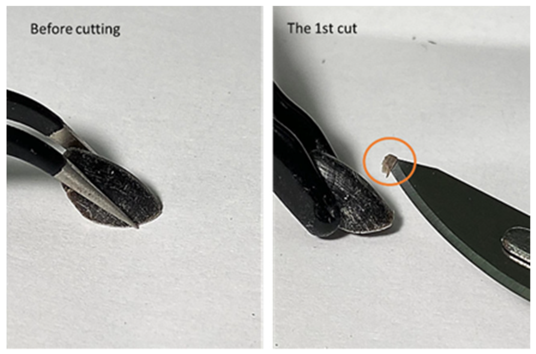
Figure 2.
The preprocessed XRD images: (a) The image after calibration; (b) The image after centering, rotation, removing hot pixels, and normalization.
Figure 2.
The preprocessed XRD images: (a) The image after calibration; (b) The image after centering, rotation, removing hot pixels, and normalization.
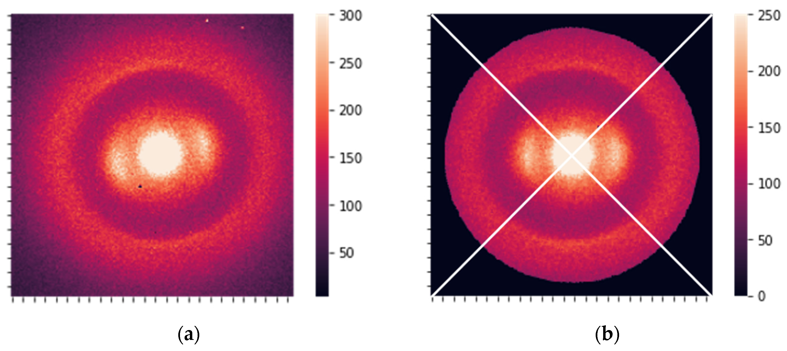
Figure 3.
ROC curves for various preprocessing steps and machine learning algorithms (the terminology is described in Section 2): (a) 2DF, LPF, BRF, Im, and RF (STD and PCA_100 for the red curve, no STD and PCA_100 for the blue curve); (b) 2DF and Am (LOG for the blue curve and RF for the red curve).
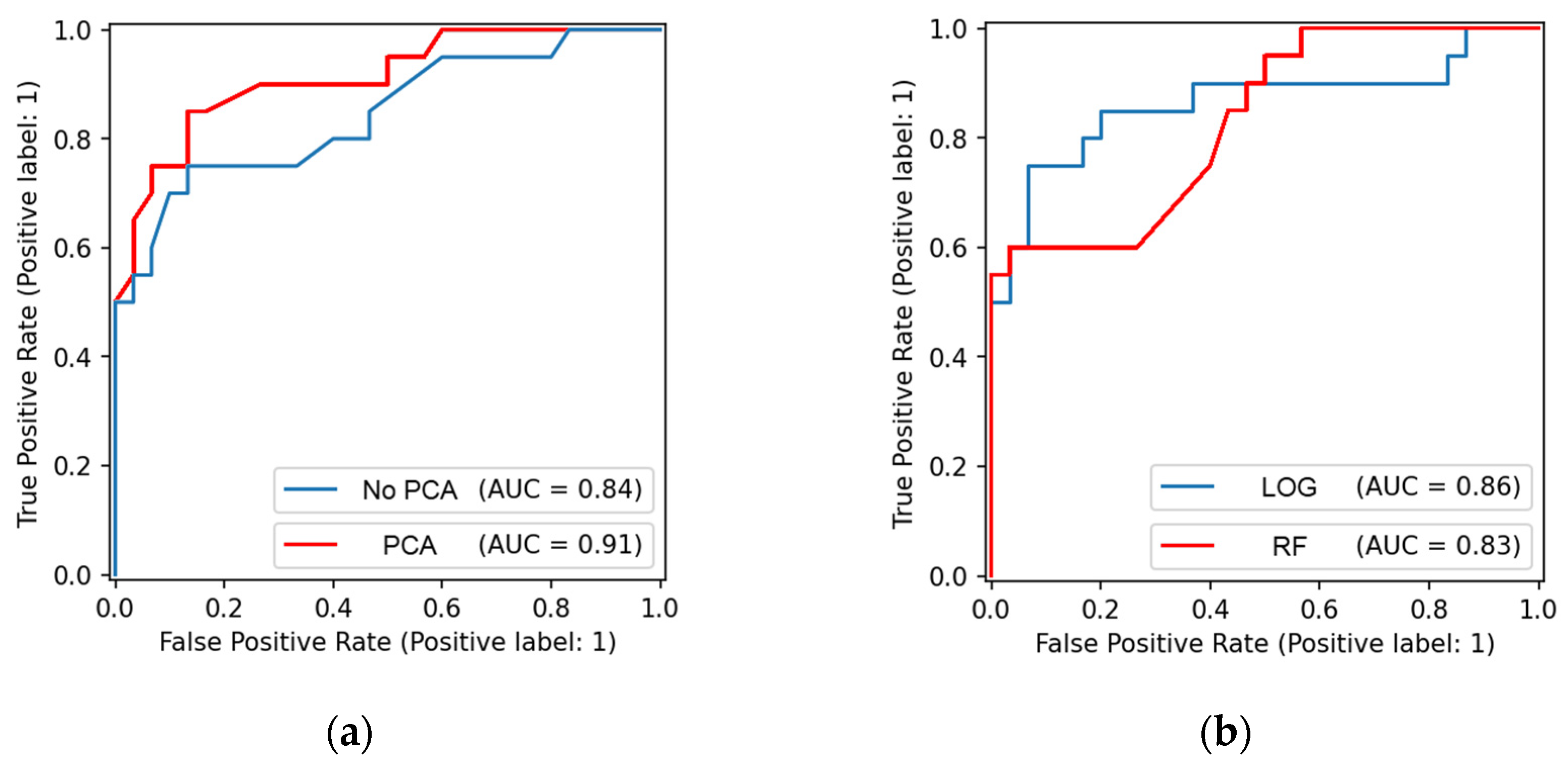
Figure 4.
PCA-transformed data in 3 dimensions for 2DF, LPF, STD, and Am with (a) BRF and (b) BR.
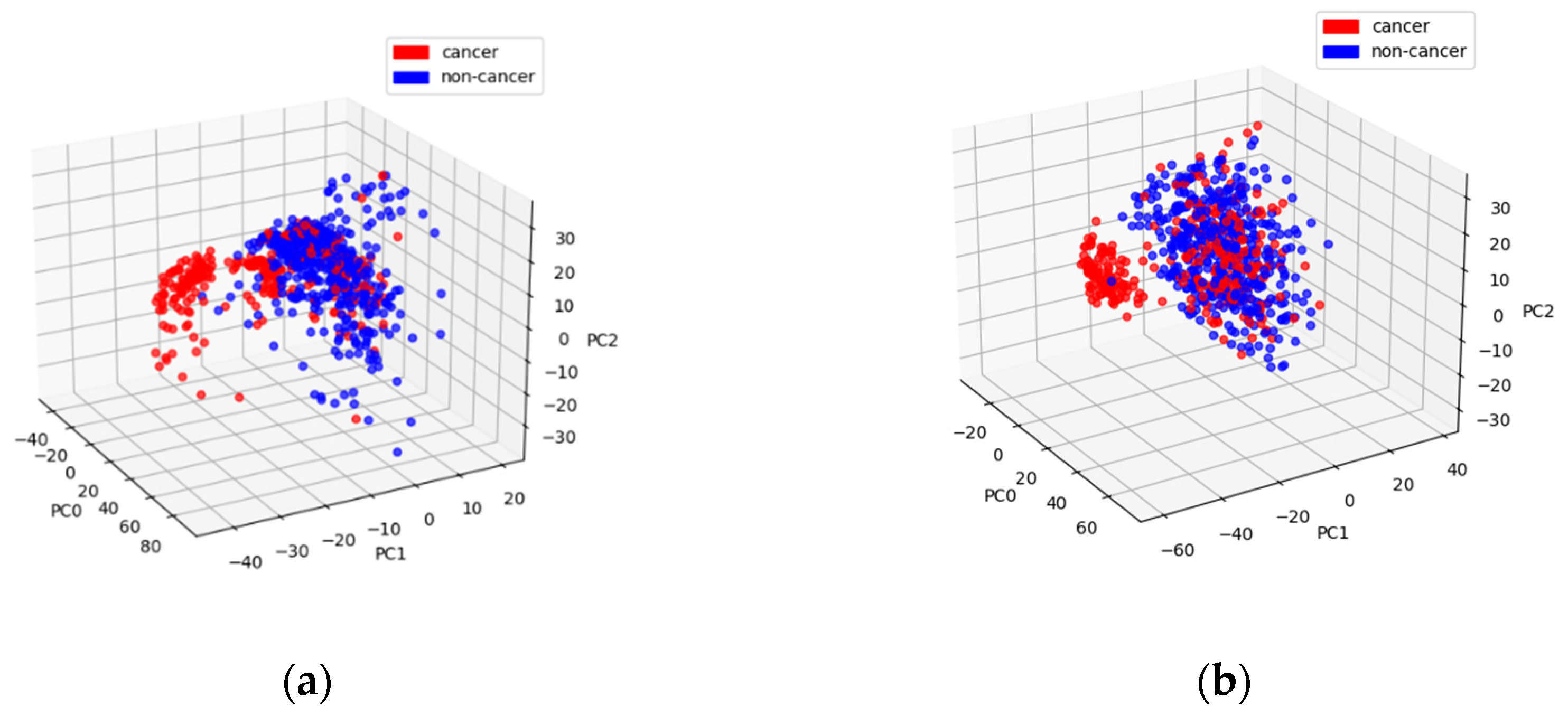

Table 1.
10 best metrics for various preprocessing steps and classifiers.
| Steps and Classifiers | Sen_S | Spec_S | AUC_S | BA_S | Sen_P | Spec_P | AUC_P | BA_P | |
|---|---|---|---|---|---|---|---|---|---|
| 1 | 2DF, BRF, LPF, STD, Im, PCA_100, RF | 0.61 | 0.95 | 0.85 | 0.78 | 0.75 | 1 | 0.93 | 0.875 |
| 2 | 2DF, BRF, LPF, STD, Re_Im, PCA_50, XGB | 0.6 | 0.88 | 0.81 | 0.74 | 0.85 | 0.87 | 0.89 | 0.86 |
| 3 | 2DF, Am, LOG | 0.64 | 0.97 | 0.81 | 0.81 | 0.75 | 0.93 | 0.86 | 0.84 |
| 4 | 2DF, BRF, LPF, STD, Im, PCA_50, XGB | 0.72 | 0.81 | 0.82 | 0.76 | 0.75 | 0.93 | 0.86 | 0.84 |
| 5 | 2DF, BR, LPF, STD, Re_Im, PCA_50, XGB | 0.57 | 0.91 | 0.81 | 0.74 | 0.75 | 0.93 | 0.87 | 0.84 |
| 6 | 2DF, BRF, LPF, STD, Re_Im, PCA_50, RF | 0.54 | 0.96 | 0.78 | 0.75 | 0.7 | 0.96 | 0.81 | 0.83 |
| 7 | 2DF, BRF, LPF, STD, Im, PCA_50, RF | 0.7 | 0.84 | 0.8 | 0.77 | 0.7 | 0.96 | 0.83 | 0.83 |
| 8 |
2DF, BR, LPF, STD, Im, PCA_50, XGB |
0.69 | 0.88 | 0.82 | 0.79 | 0.7 | 0.96 | 0.88 | 0.83 |
| 9 | 2DF, BRF, LPF, STD, Im, PCA_100, XGB | 0.72 | 0.88 | 0.83 | 0.8 | 0.9 | 0.76 | 0.87 | 0.83 |
| 10 | 2DF, LPF, Am, RF | 0.55 | 0.96 | 0.83 | 0.755 | 0.85 | 0.8 | 0.89 | 0.825 |
Table 2.
The best metrics for various preprocessing steps and classifiers not included in Table 1.
Table 2.
The best metrics for various preprocessing steps and classifiers not included in Table 1.
| Steps and Classifiers | Sen_S | Spec_S | AUC_S | BA_S | Sen_P | Spec_P | AUC_P | BA_P | |
|---|---|---|---|---|---|---|---|---|---|
| 11 | 2DF, Im, XGB | 0.52 | 0.94 | 0.76 | 0.73 | 0.75 | 0.9 | 0.81 | 0.825 |
| 15 | AI, SR, 1DFC, RF | 0.94 | 0.43 | 0.75 | 0.685 | 1 | 0.63 | 0.87 | 0.815 |
| 16 | AIS, SR, 1DFC, RF | 0.79 | 0.69 | 0.8 | 0.74 | 0.9 | 0.73 | 0.88 | 0.815 |
| 21 | 2DF, BRF, STD, Re, PCA_3, RF | 0.73 | 0.74 | 0.75 | 0.735 | 0.75 | 0.87 | 0.84 | 0.81 |
| 27 | AI, SR, 1DF, XGB | 0.65 | 0.77 | 0.72 | 0.71 | 0.65 | 0.97 | 0.78 | 0.81 |
| 103 | 2DF, BR, LPF, STD, Re_Im, PCA_750, RF | 0.66 | 0.7 | 0.73 | 0.68 | 0.95 | 0.6 | 0.84 | 0.775 |
Table 3.
The best metrics for various preprocessing steps and classifiers with the additional condition that the sensitivity is greater than 0.9.
Table 3.
The best metrics for various preprocessing steps and classifiers with the additional condition that the sensitivity is greater than 0.9.
| Steps and Classifiers | Sen_S | Spec_S | AUC_S | BA_S | Sen_P | Spec_P | AUC_P | BA_P | |
|---|---|---|---|---|---|---|---|---|---|
| 1 | 2DF, BRF, LPF, STD, Im, PCA_100, RF | 0.94 | 0.34 | 0.85 | 0.64 | 0.9 | 0.83 | 0.93 | 0.865 |
| 2 | 2DF, BRF, LPF, STD, Im, PCA_100, XGB | 0.91 | 0.41 | 0.83 | 0.66 | 0.9 | 0.77 | 0.87 | 0.83 |
| 3 | AI, SR, 1DFC, RF | 0.94 | 0.43 | 0.75 | 0.685 | 1 | 0.63 | 0.87 | 0.815 |
| 4 | AIS, SR, 1DFC, RF | 0.95 | 0.23 | 0.8 | 0.59 | 0.9 | 0.73 | 0.88 | 0.815 |
| 5 | 2DF, Am, RF | 0.93 | 0.37 | 0.83 | 0.65 | 0.9 | 0.73 | 0.89 | 0.815 |
Table 4.
The best metrics for various preprocessing steps and classifiers with the additional condition that the specificity is greater than 0.9.
Table 4.
The best metrics for various preprocessing steps and classifiers with the additional condition that the specificity is greater than 0.9.
| Steps and Classifiers | Sen_S | Spec_S | AUC_S | BA_S | Sen_P | Spec_P | AUC_P | BA_P | |
|---|---|---|---|---|---|---|---|---|---|
| 1 | 2DF, BRF, LPF, STD, Im, PCA_100, RF | 0.61 | 0.95 | 0.85 | 0.78 | 0.75 | 1 | 0.93 | 0.875 |
| 2 | 2DF, BRF, LPF, Im, XGB | 0.61 | 0.9 | 0.79 | 0.755 | 0.65 | 1 | 0.84 | 0.825 |
| 3 |
2DF, BR, STD, Am, PCA_50, RF |
0.63 | 0.91 | 0.8 | 0.77 | 0.6 | 1 | 0.83 | 0.8 |
| 4 |
2DF, BR, LPF, STD, Re_Im, PCA_50, XGB |
0.54 | 0.94 | 0.79 | 0.74 | 0.6 | 1 | 0.81 | 0.8 |
| 5 | 2DF, LPF, Re_Im, XGB | 0.55 | 0.92 | 0.79 | 0.735 | 0.55 | 1 | 0.82 | 0.775 |
Disclaimer/Publisher’s Note: The statements, opinions and data contained in all publications are solely those of the individual author(s) and contributor(s) and not of MDPI and/or the editor(s). MDPI and/or the editor(s) disclaim responsibility for any injury to people or property resulting from any ideas, methods, instructions or products referred to in the content. |
© 2024 by the authors. Licensee MDPI, Basel, Switzerland. This article is an open access article distributed under the terms and conditions of the Creative Commons Attribution (CC BY) license (http://creativecommons.org/licenses/by/4.0/).
Copyright: This open access article is published under a Creative Commons CC BY 4.0 license, which permit the free download, distribution, and reuse, provided that the author and preprint are cited in any reuse.


