Submitted:
21 November 2024
Posted:
22 November 2024
You are already at the latest version
Abstract
Ethanol has always been an integral part of our daily life. We often use ethanol knowingly or unknowingly in many formats. Industrialists use ethanol as a primary or secondary solvent in the synthesis of organic materials, as a cleaning/ sanitising solvent which can sanitise the area where it is applied onto. As a fuel, ethanol can be used as an additive to standard gasoline to make the fuel cleaner and greener. A greener commute/ travel is currently possible dominantly with the usage of electric vehicles (EVs). However, the EV infrastructure is in the primitive stages where the growth is not that exceptional as it expected but there is a steady growth. To catch up with the conventional fuels, it would take a considerable amount of time. In order to cut down the carbon footprint in the present, the addition of green additives in the fuels are the suggested actions. With countries like India initiating the action to bring down the gasoline consumption by increasing the ethanol content to a 20% by 2030, there is a good market for additives like ethanol and butanol which can be produced using a green way. There is also a concern with backwards compatibility of the EV with fuel which is not compatible. To make majority of the vehicles cleaner and greener bio-based additives are the go-to. The necessity of biofuels due to the reasons above has increased in the recent years which led to an increase in the production and the costs associated with the production. To cut down the costs associated with the production; process intensification techniques are utilised to reduce the time to process the raw materials to products. Intensification techniques like reactive distillation, pervaporation had been the norm to perform two-unit operations in the same machinery. In the recent years with the introduction of microbubbles, the addition of hot microbubbles has solved the long unsolved Mpemba effect along with the ability to perform multiple unit operations altogether. This project aspires to develop a Multiphysics model where the modelled system initially represents a single air microbubble in a reservoir of a binary mixture of ethanol and water in a 2-D axisymmetric domain and perform a parametric sweep on the bubble to incorporate hotter bubbles and observe its behaviour. The model is scaled up to a two-bubble system to find the optimum separation of bubbles where interaction is nil and the heat distribution I even across the system. A 3-D geometry is generated with the simulation from the 2-bubble system using the optimal distance where bubbles are generated using COMSOL’s application builder to build the ideal microbubble system and simulate the same.
Keywords:
Chapter 1: Introduction
1.1. Background
1.1.1. Bioethanol

| S. No | Property | Value/Description |
|---|---|---|
| 1 | Boiling point | 78.37℃ |
| 2 | Flammability | Highly flammable |
| 3 | Molecular weight | 46.068 g/mol |
| 4 | Formula | C2H5OH |
| 5 | IUPAC Name | Ethyl Alcohol |
| 6 | Azeotrope Point | 78℃ and 95.5% ethanol and rest water |
1.1.2. Microbubbles
1.1.3. Multiphysics Modelling and COMSOL
1.2. Overview
Chapter 2: Literature Survey
2.1. General Survey
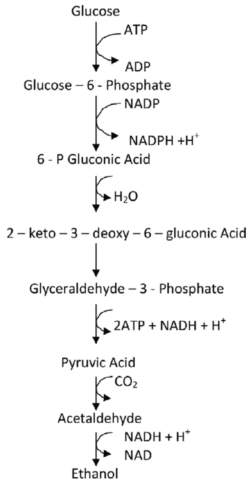
2.2. Production of Bioethanol
- 1)
-
Reduced complexity of the process:Using direct sugars which are sucrose and glucose mix, the complexity of the process decreases drastically. When using cellulosic materials as a source of raw material, they need to be pre-processed in order to be converted to glucose and remove undesirable materials like hemi and holo celluloses [20].The pre-treatment of the raw materials can be a time taking process where the raw materials are hydrolysed to remove the undesirable substances and to convert lignocellulose into glucose. The process can be heavy on manpower and energy as well.Using direct sugars to produce ethanol can be a lesser complex process which needs lesser equipment which often leads to lower capital investment by the manufacturers.
- 2)
-
Decreased costs associated with production:Cost can contribute to a huge factor in determining things as one cannot simply go behind “green” and “sustainable” production. This is a main reason why producers usually go with synthetic ethanol rather than bioethanol as the costs associated with production is far cheaper than compared to bioethanol as discussed in Li et.al [3]. Higher costs to the production are usually not favoured by the manufacturers as they tend to be recurring and not a one-time investment. Added process line involving pre-treatment of raw materials can increase the costs associated as the operators need to maintain the process at a certain temperature to properly pre-treat.For the fermentation alone, O2 supply as described by Raghavendran et.al [5] accounts to up to 15% of the total cost of production. In order to reduce the costs associated to production, process intensification techniques are utilised. In certain cases in pharmaceutical production units, the reaction takes place in a pressurised vessel or a jacketed vessel where post reaction process, the undesirable or the desirable is extracted in the same vessel by heating the unit or decreasing or increasing the pressure for volatile products and also could perform liquid-liquid extractions to remove undesirable or desirable products depending on the process.
- 3)
-
Surplus of sugar stocks:India is currently the largest producer of sugar and the third largest exporter of sugar. This means that the country is producing the most sugar and is exporting a small fraction of sugar which leaves a huge surplus in the sugar stock in the Indian godowns. An estimate of around 35 lakh tonnes or 3.5 million tonnes of sugar is produced in excess [23]. With the excess in mind, the resources are more than sufficient to keep its citizens supplied with sugar and also focus on the blended fuel which is termed as ethanol blending program (EBP).Although there is a hitch where the sugarcane is a seasonal harvest which is planted in the months of December through March and is harvested in the months of January through March. This leaves with a limited supply of sugarcane throughout the year and the plants being operational only in few months of the year i.e., during the harvest period, the main challenge is to store the produced sugars suitable for ethanol production throughout the year.This might be a temporary feather in the cap for India as the farmers are distressed/ dissatisfied on the prices offered for their crops by the private authorities and the government authorities, the farmers are bailing out from planting a sugarcane crop. [26]
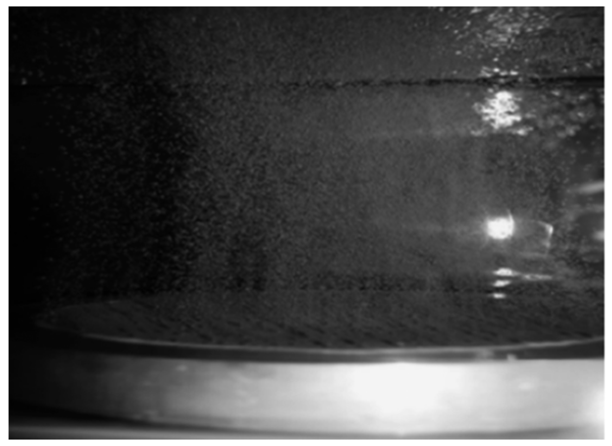
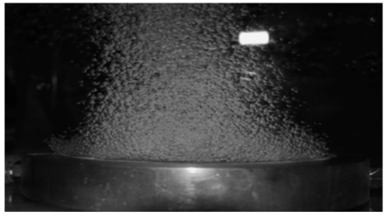
2.3. Microbubbles
- ○
- Surface tensions on the bubbles prevent any deformities to occur on the bubble’s surface due to the size of the bubbles.
- ○
- A fully laminar flow is achieved instantaneously.
| Model | Equation |
|---|---|
| Internal Velocity |
|
| Mass Transport | |
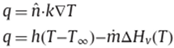
| Heat Transfer | |
| Partial Pressure |
|
| Boundary Condition | 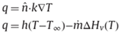 |
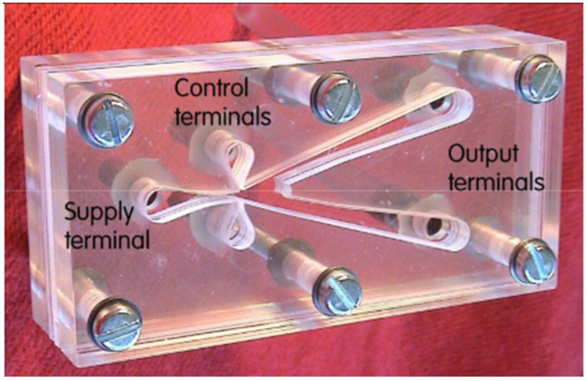
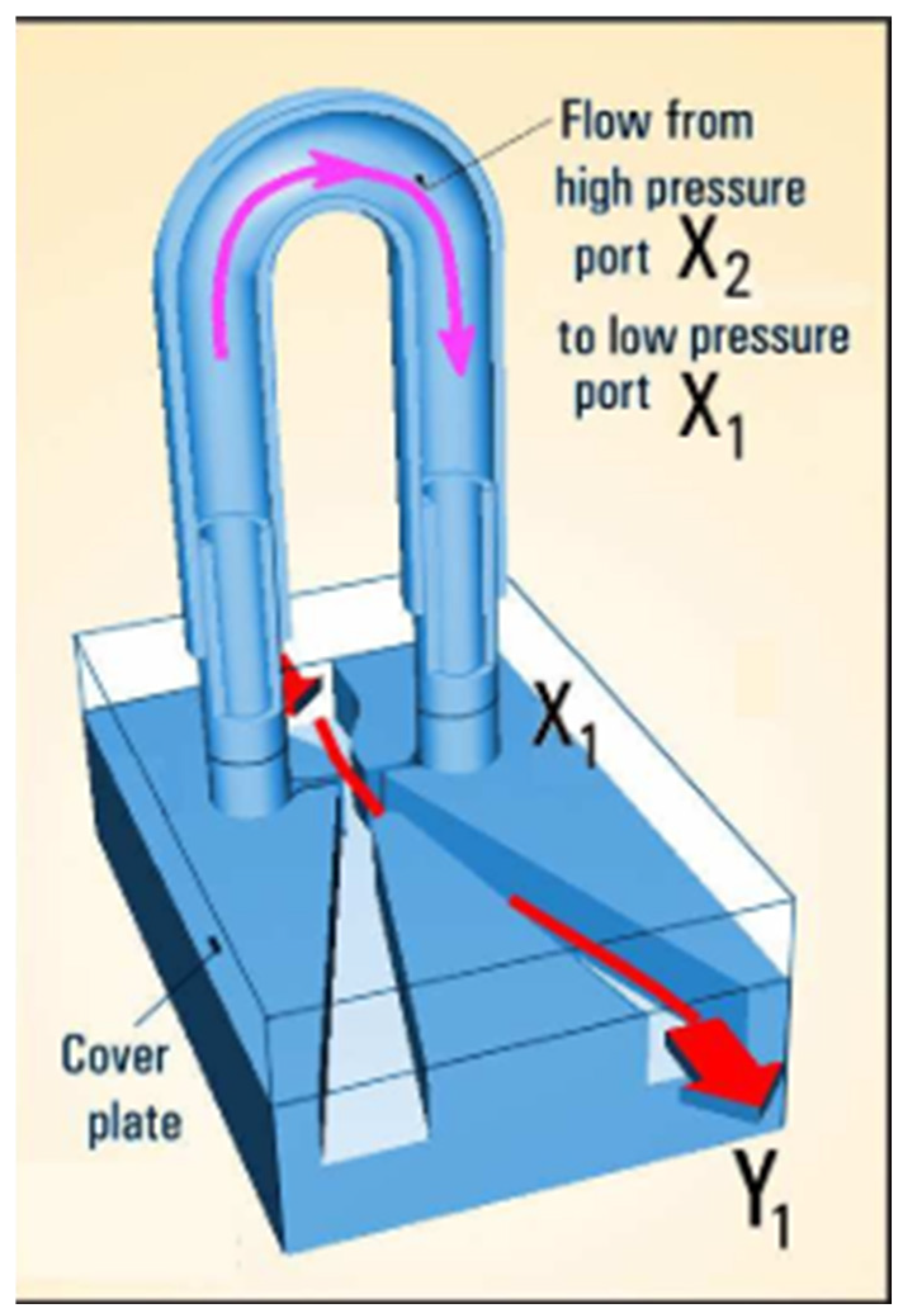
2.4. Microbubble Generation
2.5. Multiphysics Modelling and COMSOL
Chapter 3: Research Methods
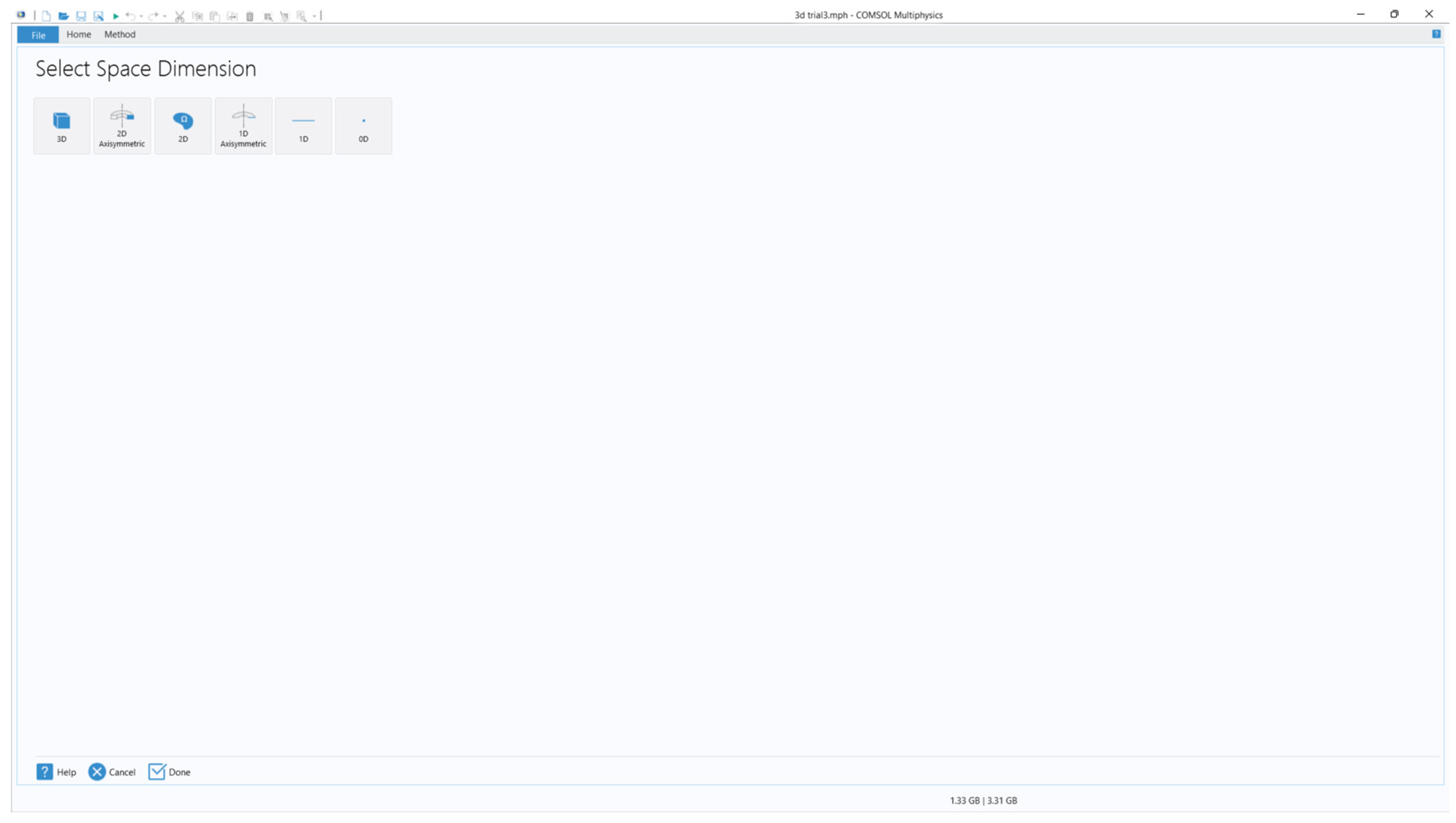
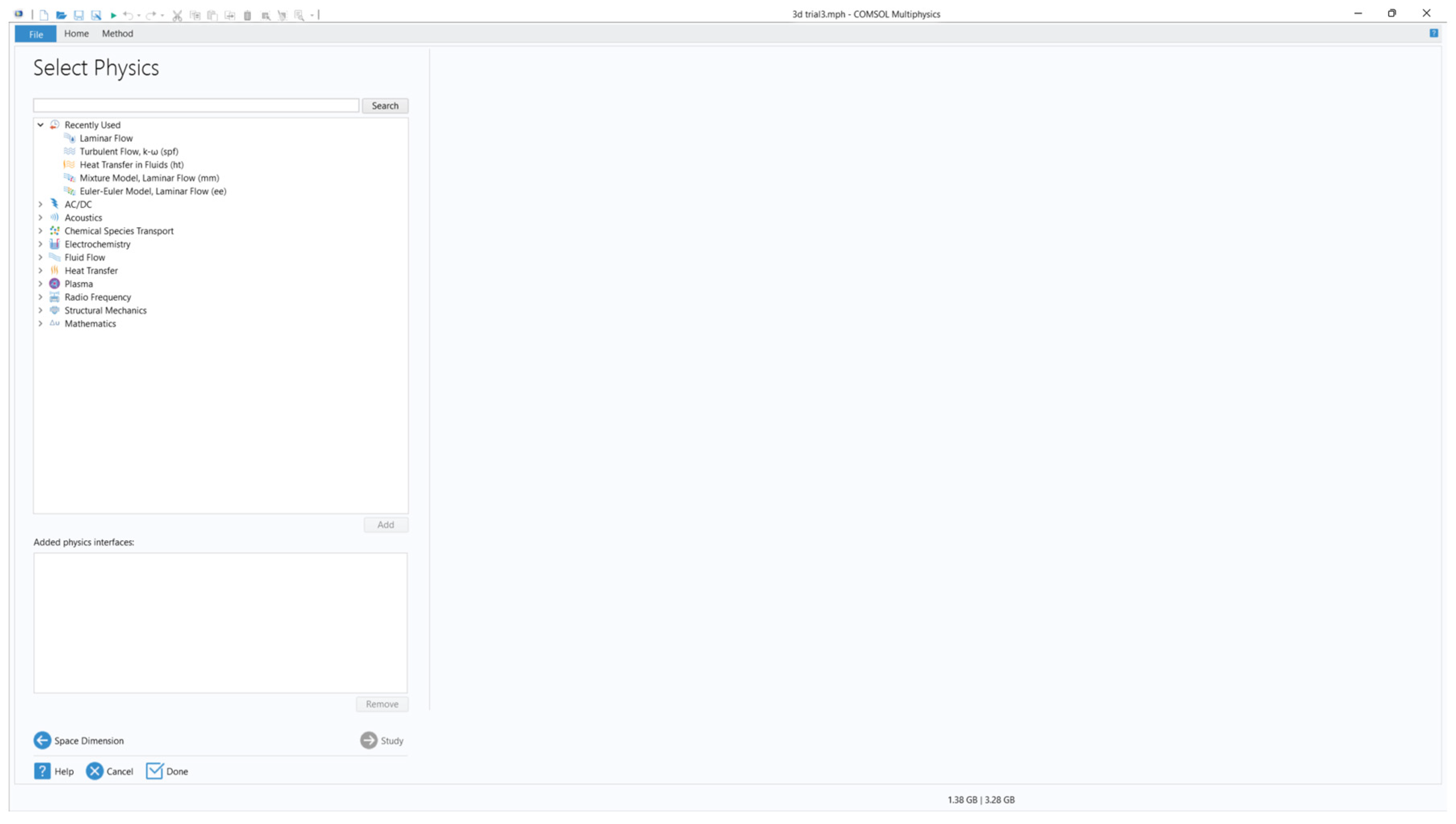
3.1. A Brief to COMSOL
3.2. Model Equations
- The bubbles are small enough that the surface tensions exerted by the bubbles oppose any deformations to the spherical shape.
- The time to achieve a fully developed laminar flow is instantaneous so that laminar flow can be considered throughout the model and the travel of the bubble.
- The bubbles act individually and does not merge into each other to form larger bubbles.
- The bubbles are shaped evenly and are sized and spaced equally to reduce complications and travels parallel to the z-axis.
- 1)
- Fluid dynamics:
- 2)
- Heat and mass transfers:
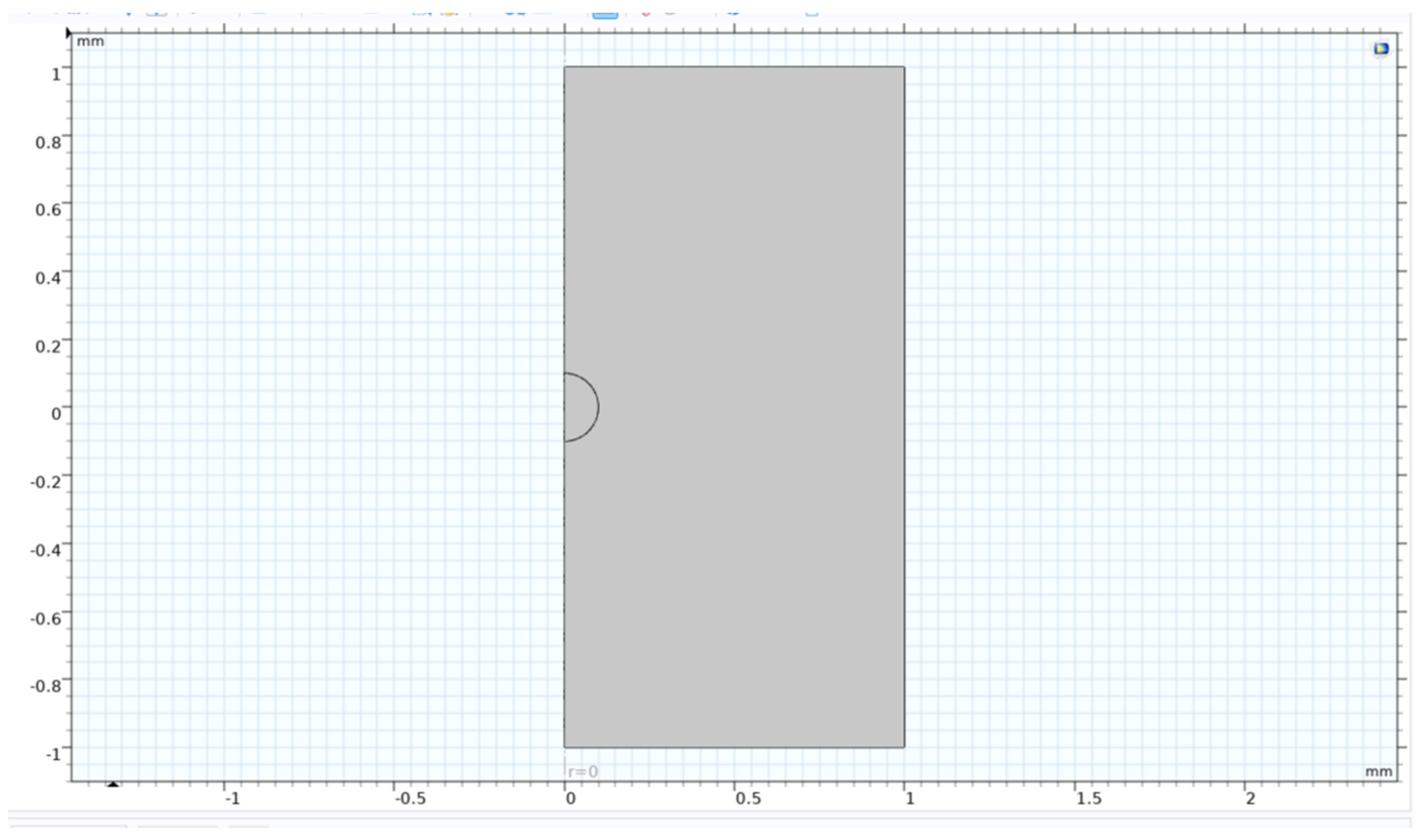
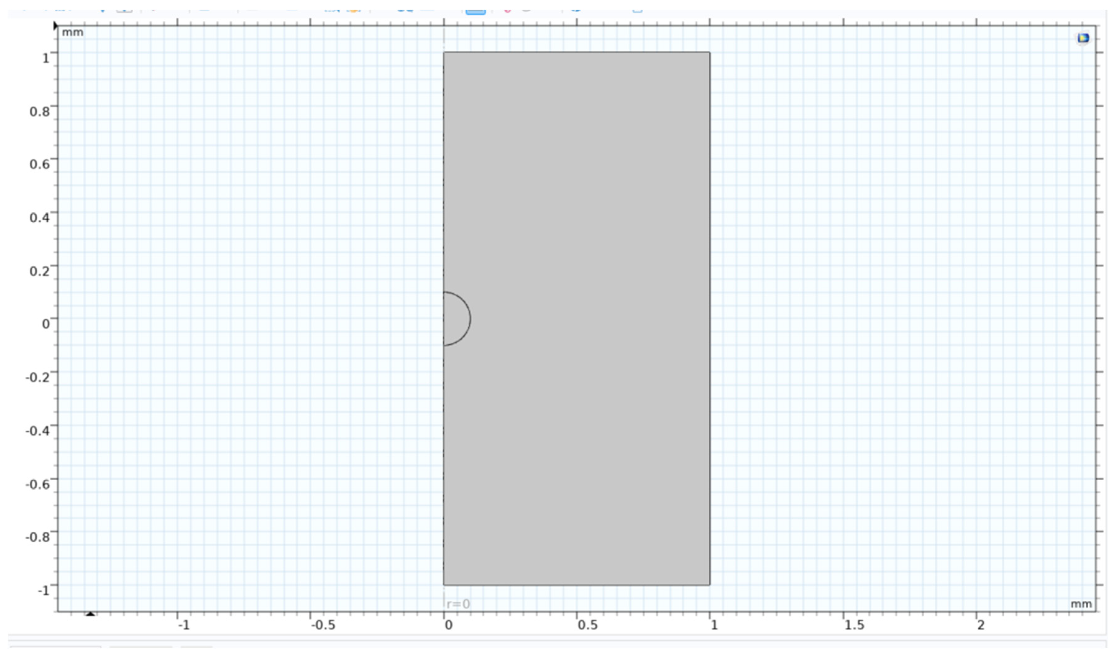
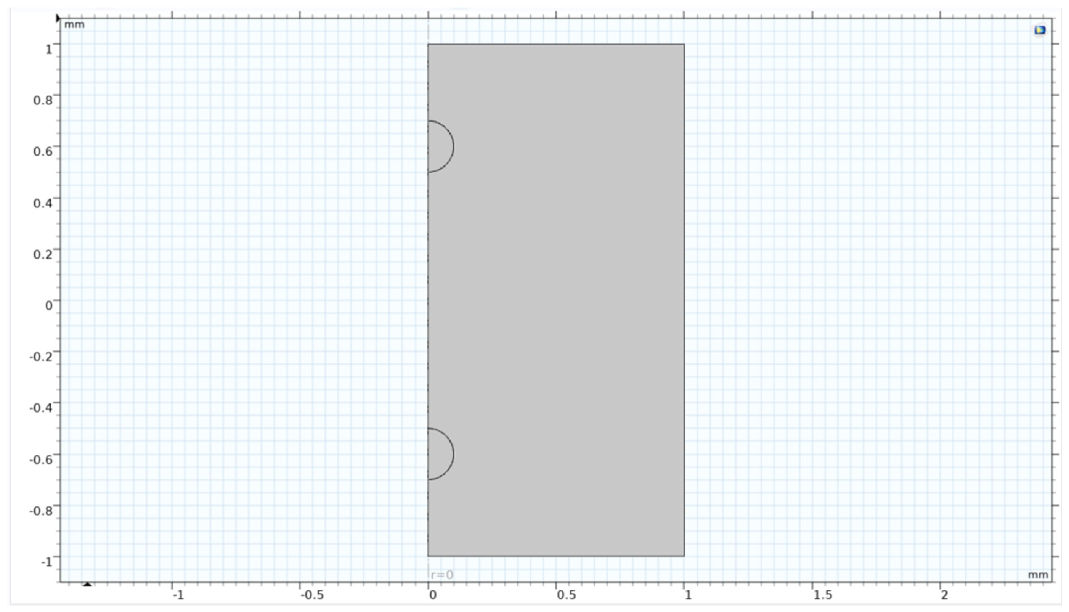
3.3. Model Set-Up
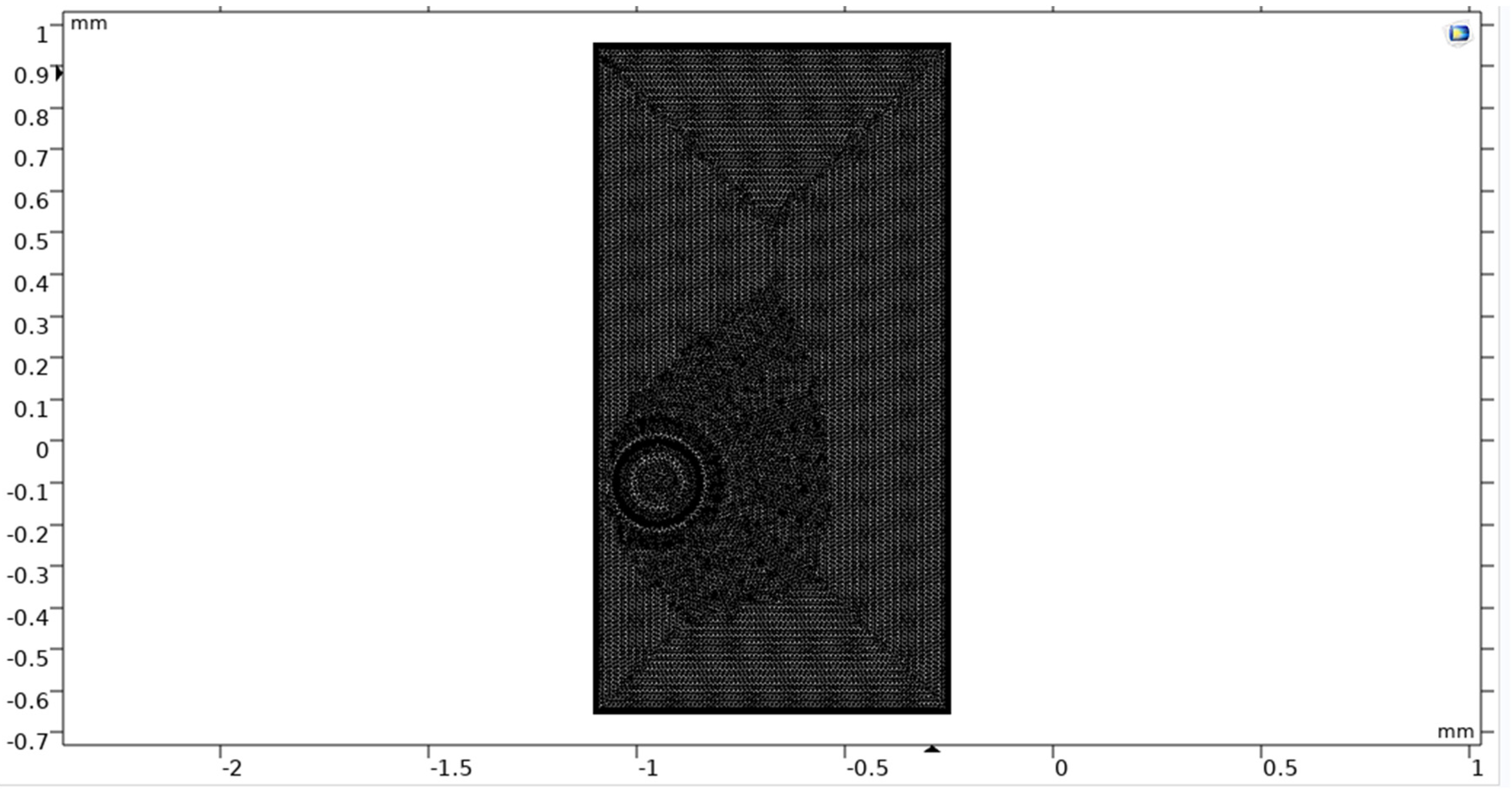
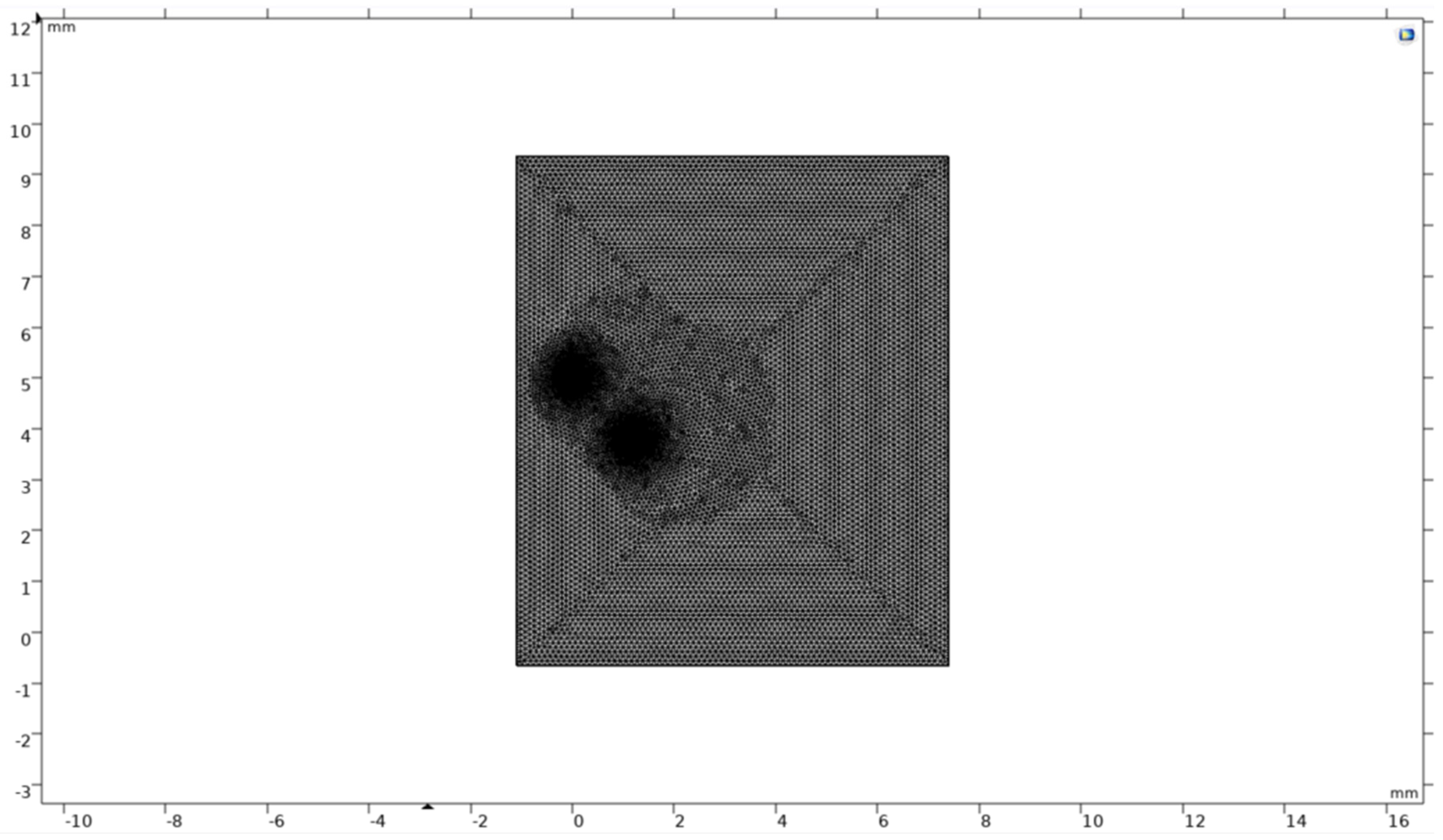
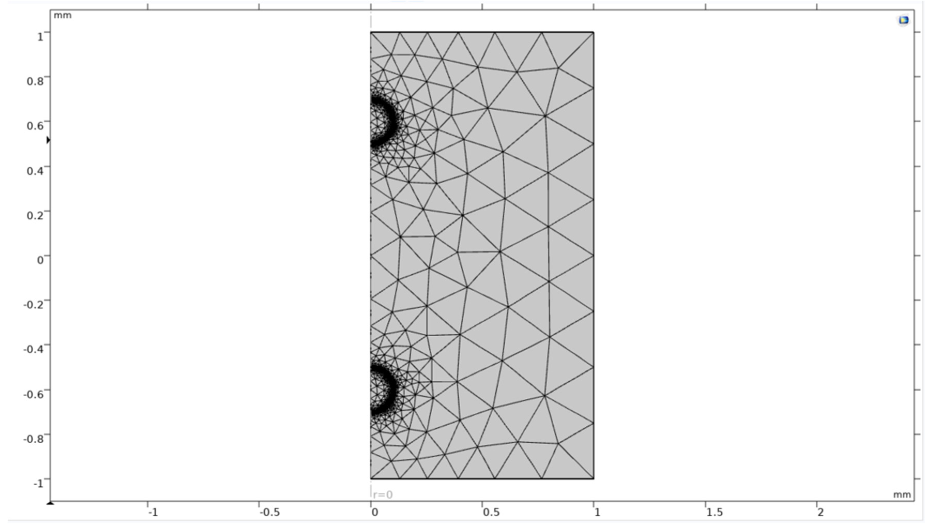
3.4. Mesh Selection and Meshing
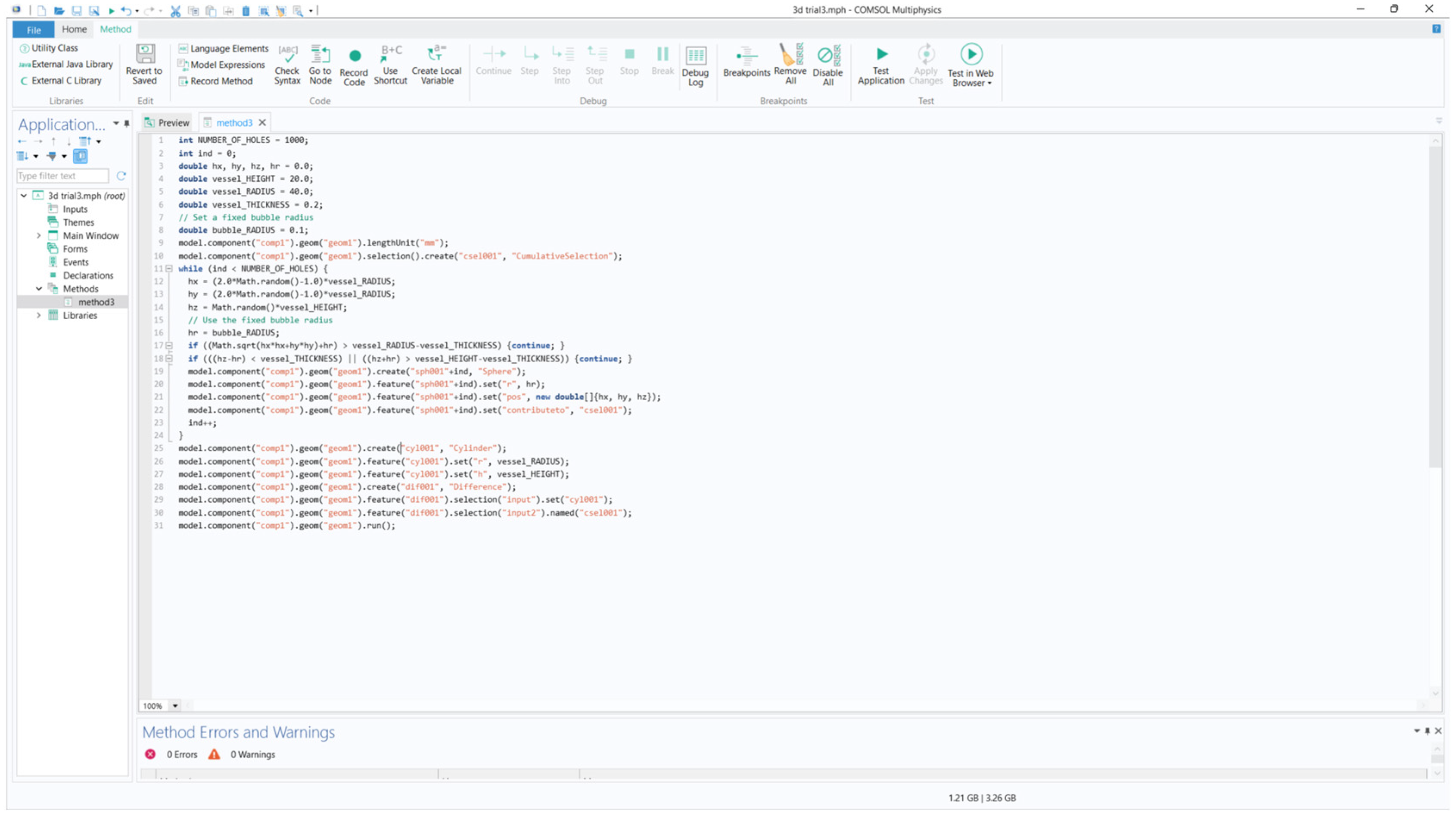
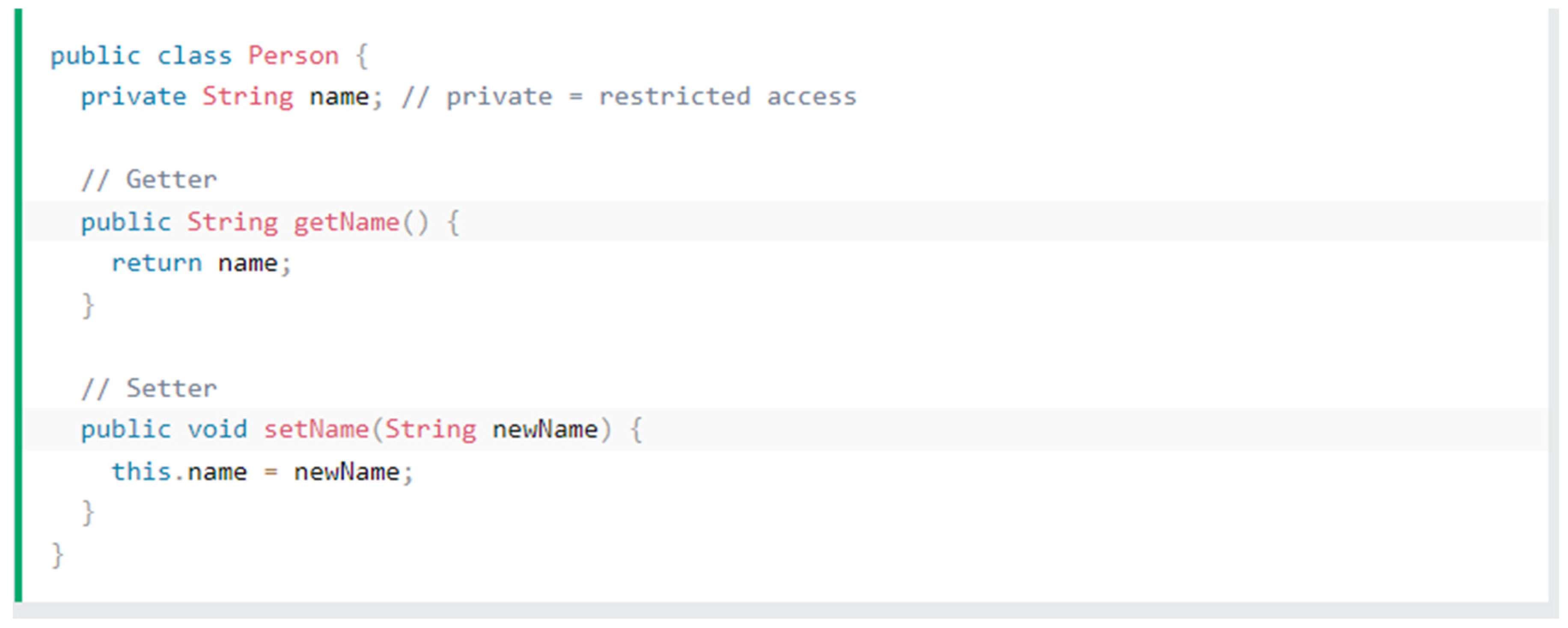
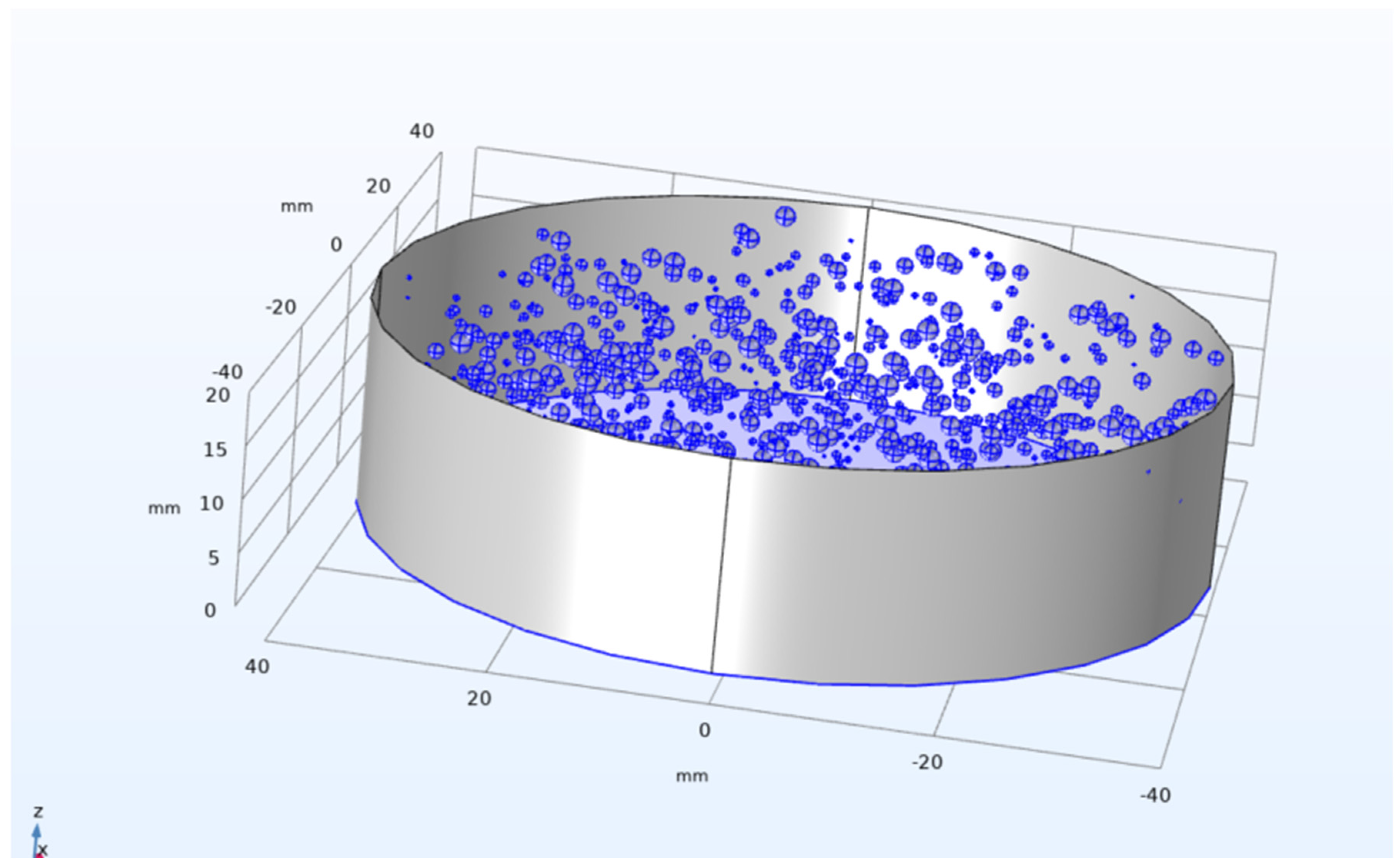
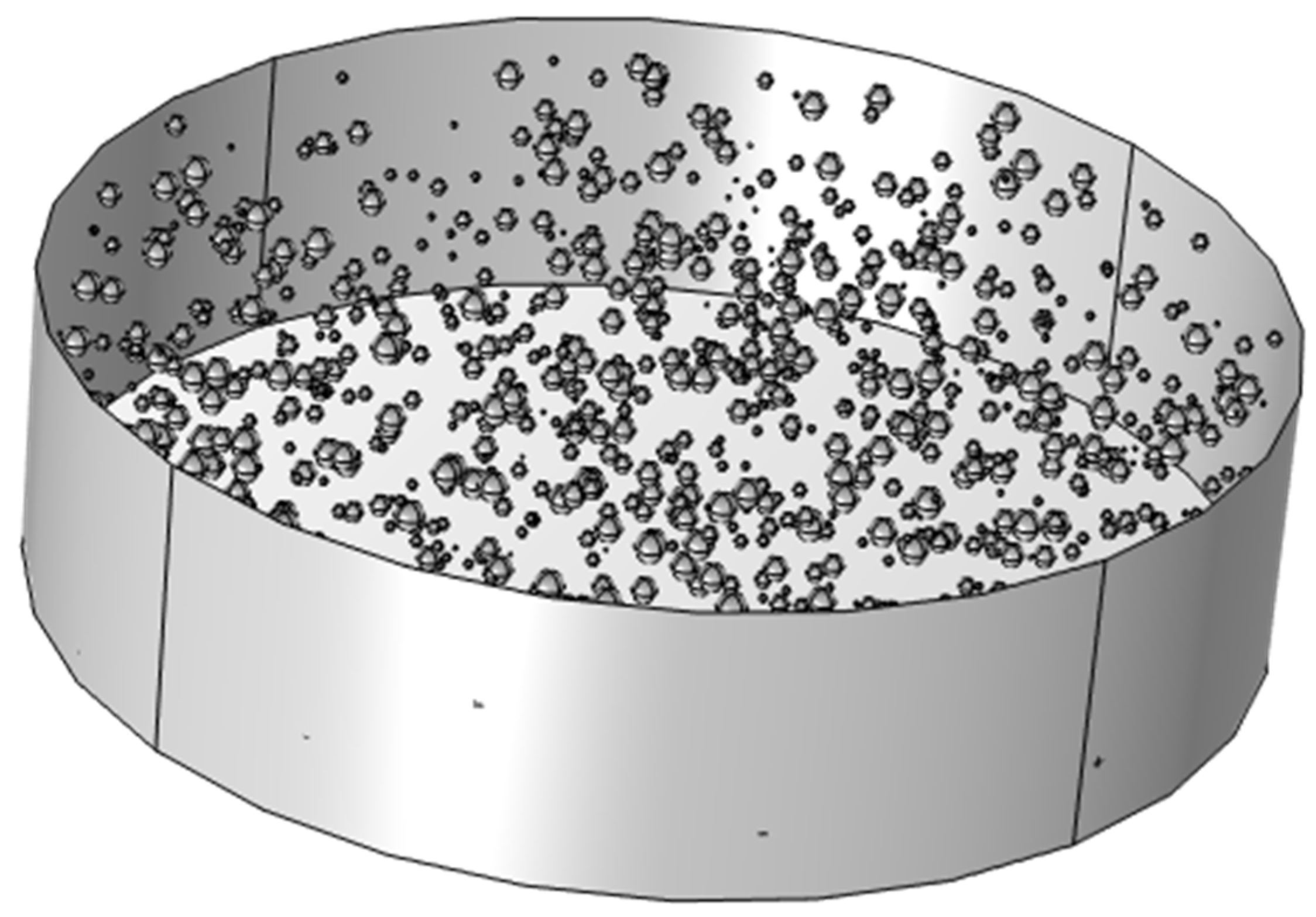
3.5. Application Builder
3.6. Model Studies
3.7. Overall Methodology
Chapter 4: Results
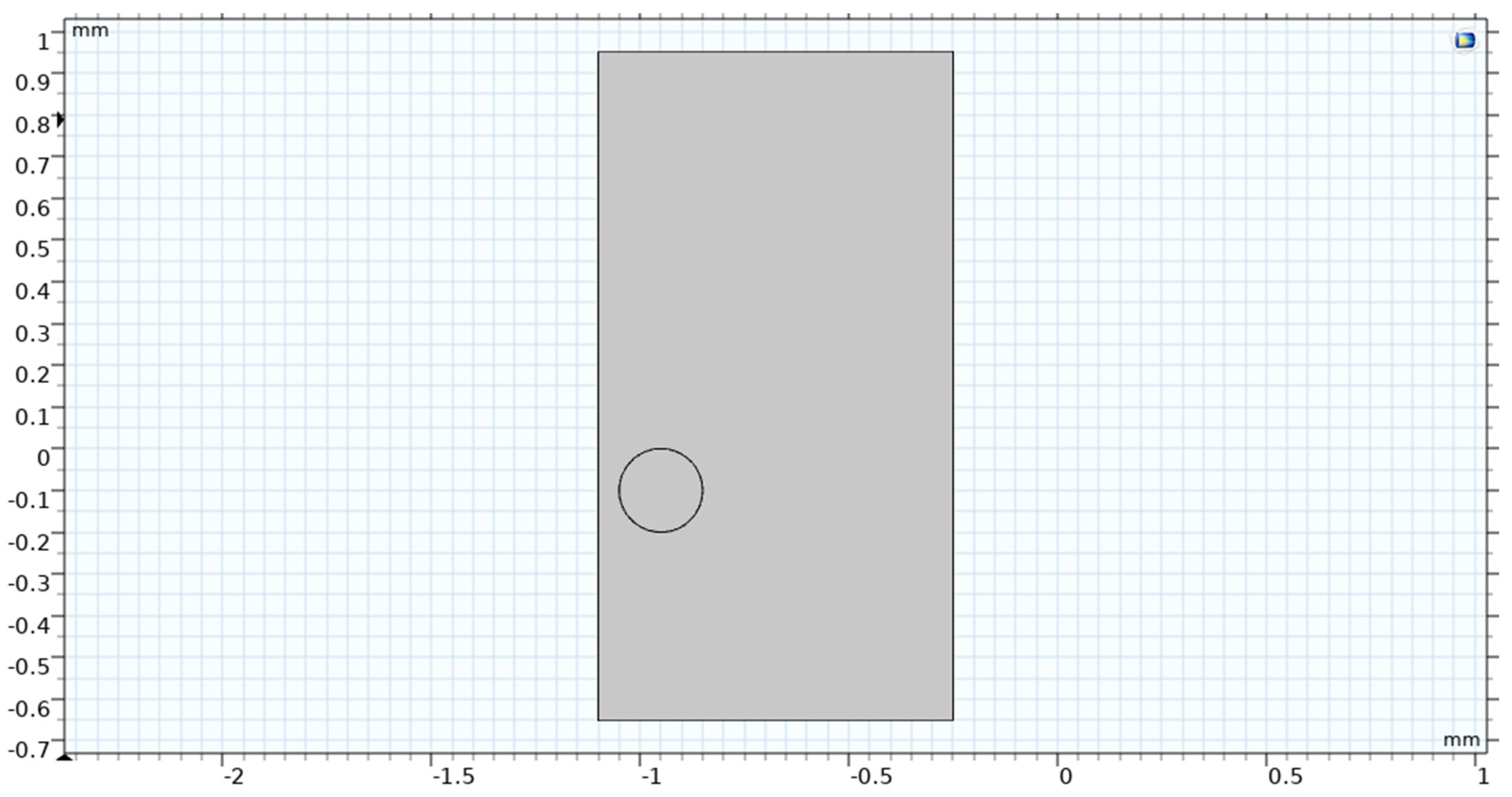
4.1. Initial Test
- 1)
- Test the features available in COMSOL available with respect to microbubbles.
- 2)
- Check the residence time of microbubbles in the reservoir.
- 3)
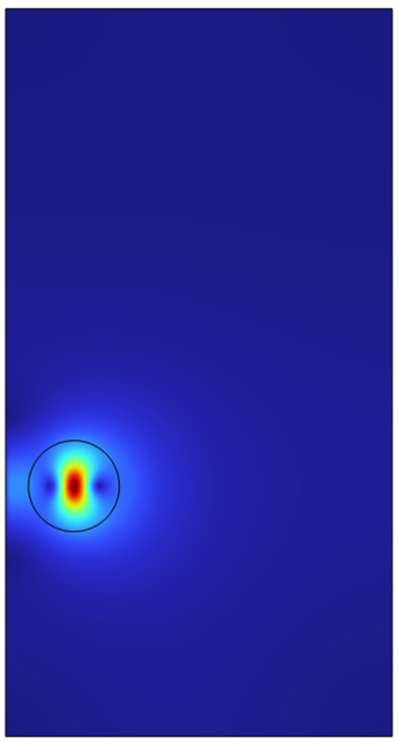
- Study the fluid dynamic effects of the single microbubble system in a 2-D plane.
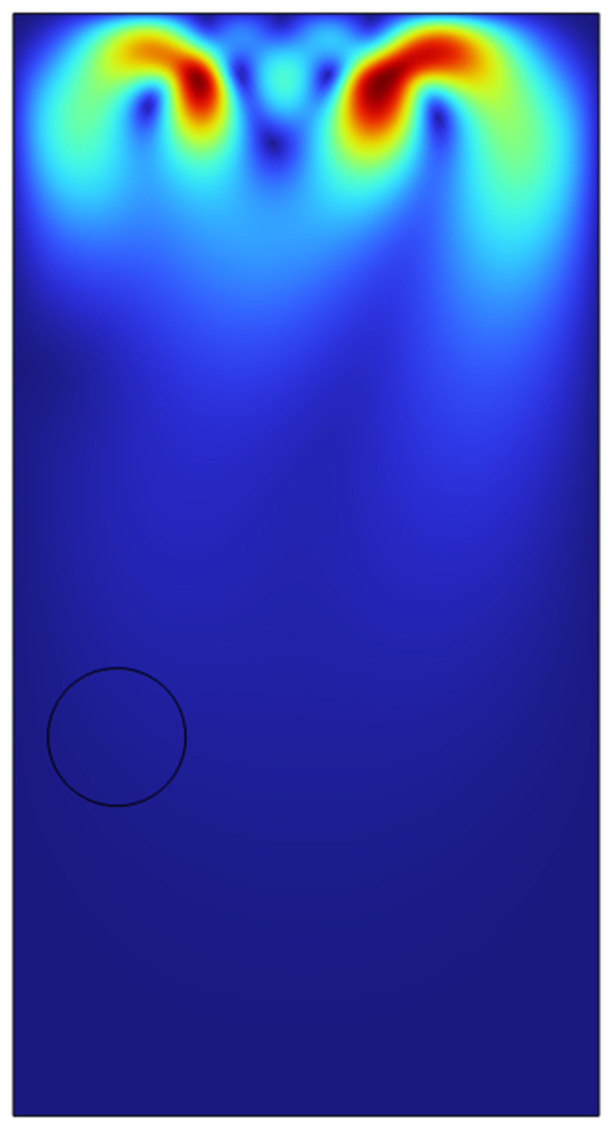
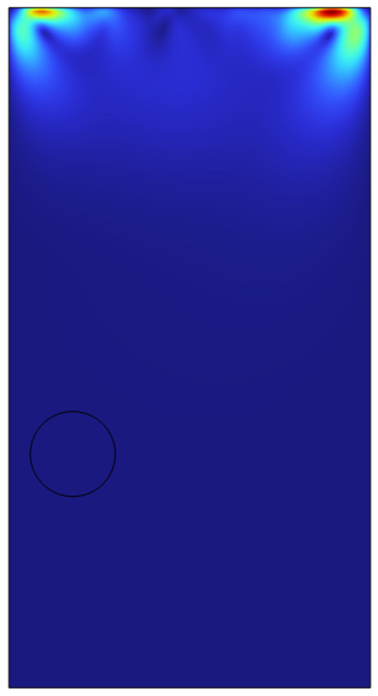
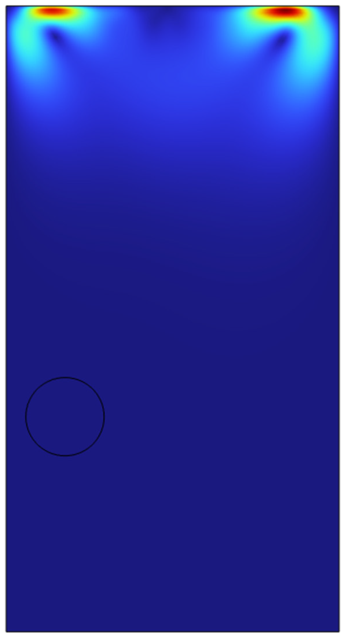
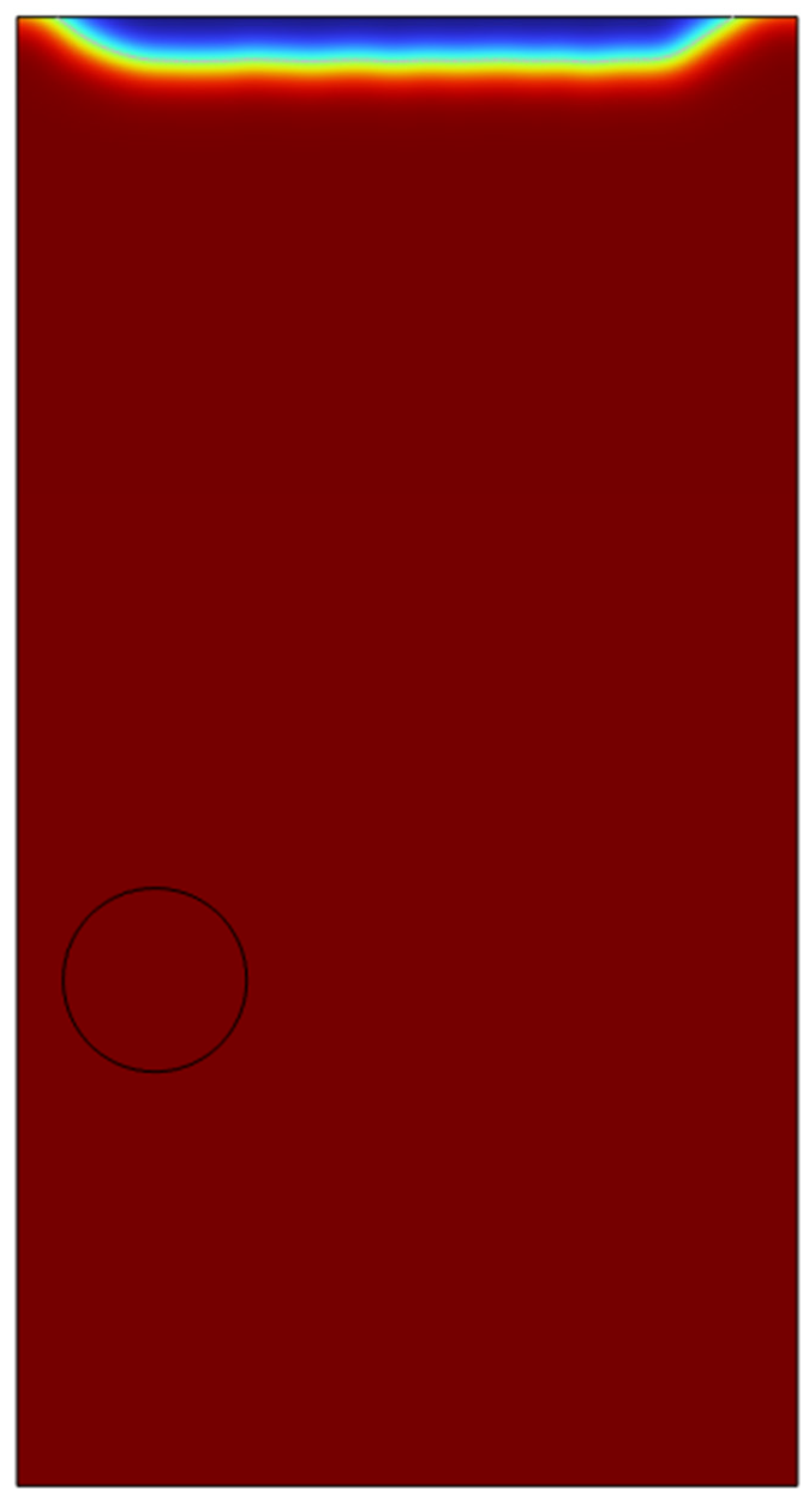
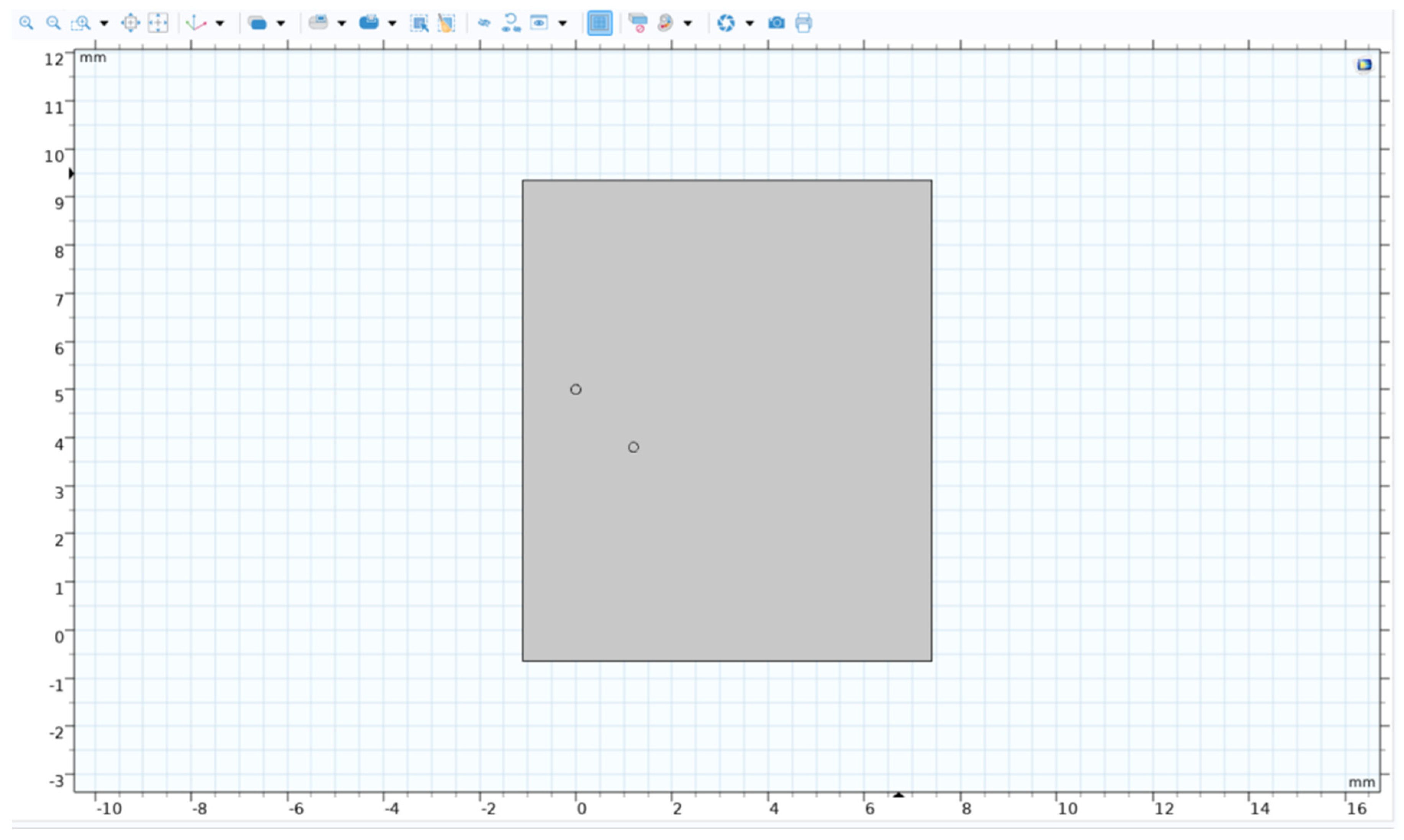
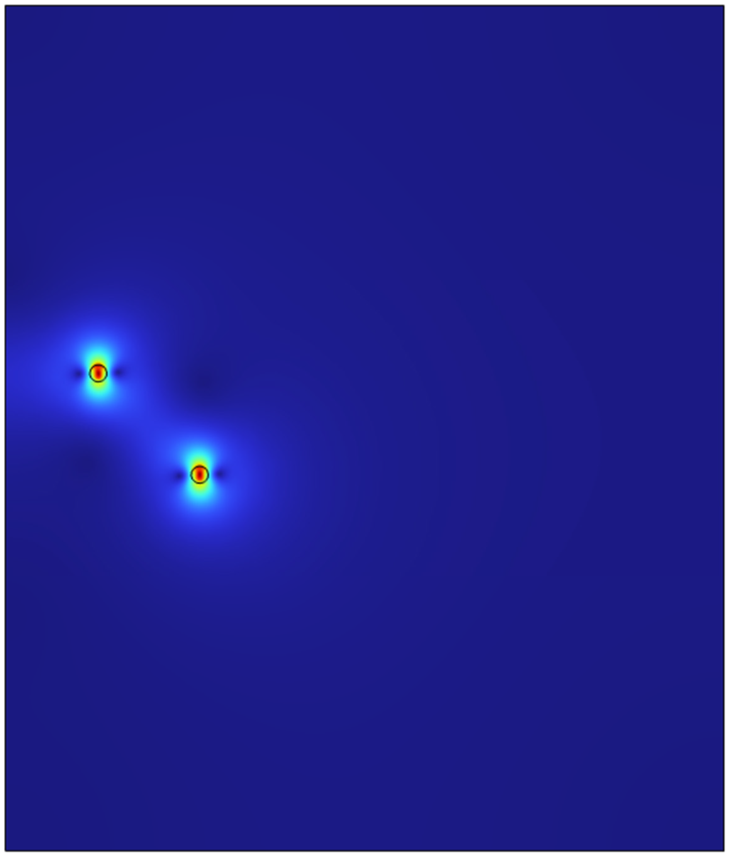
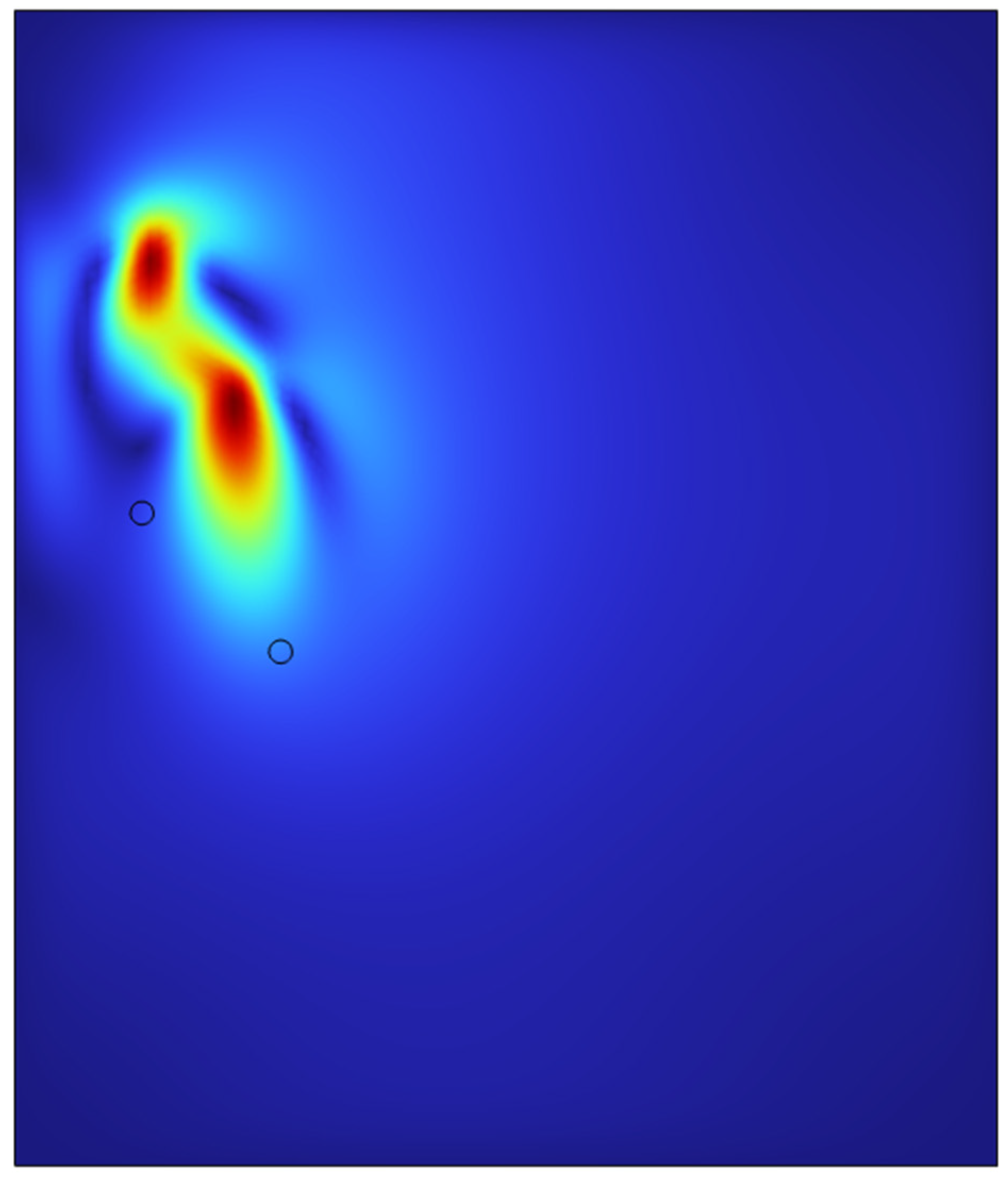
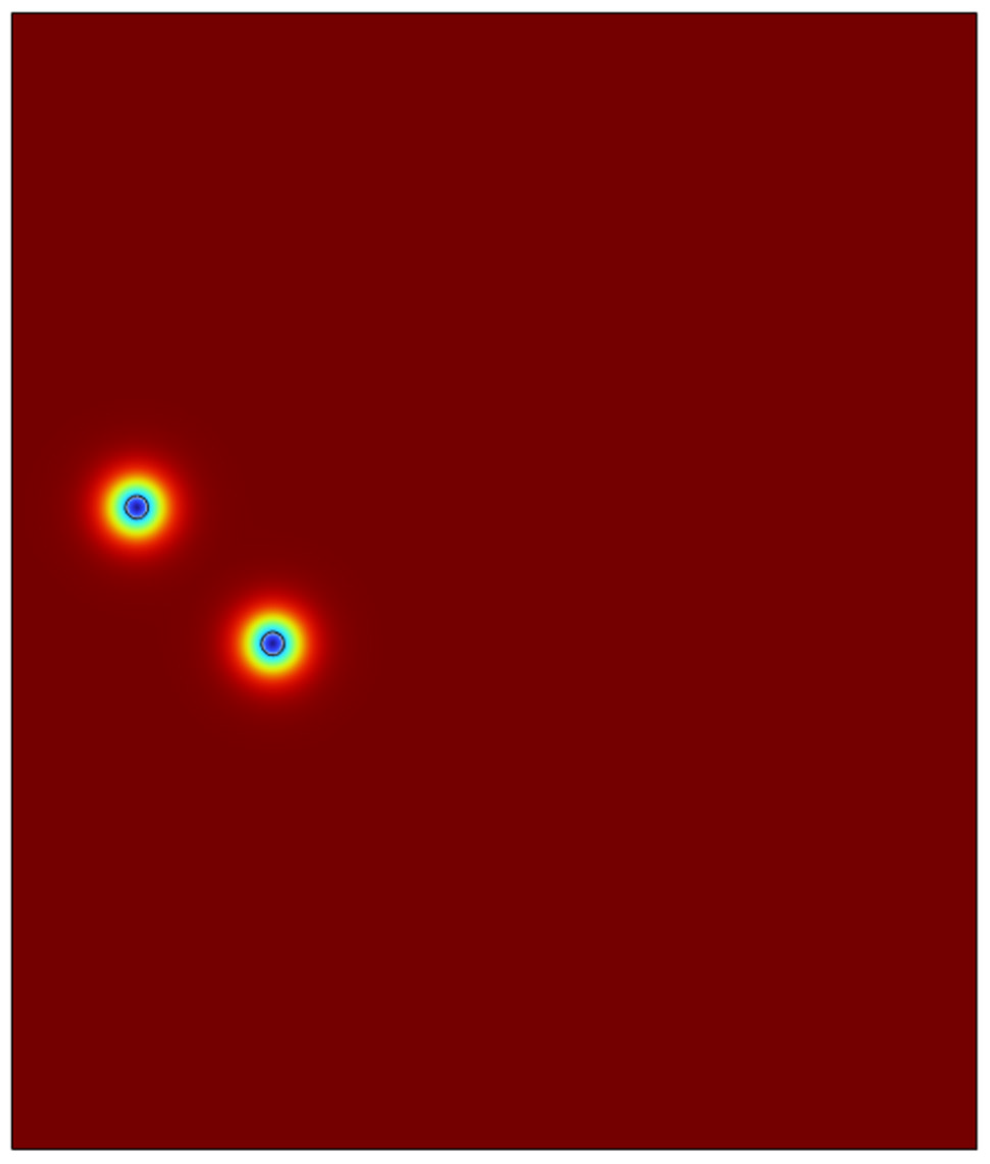
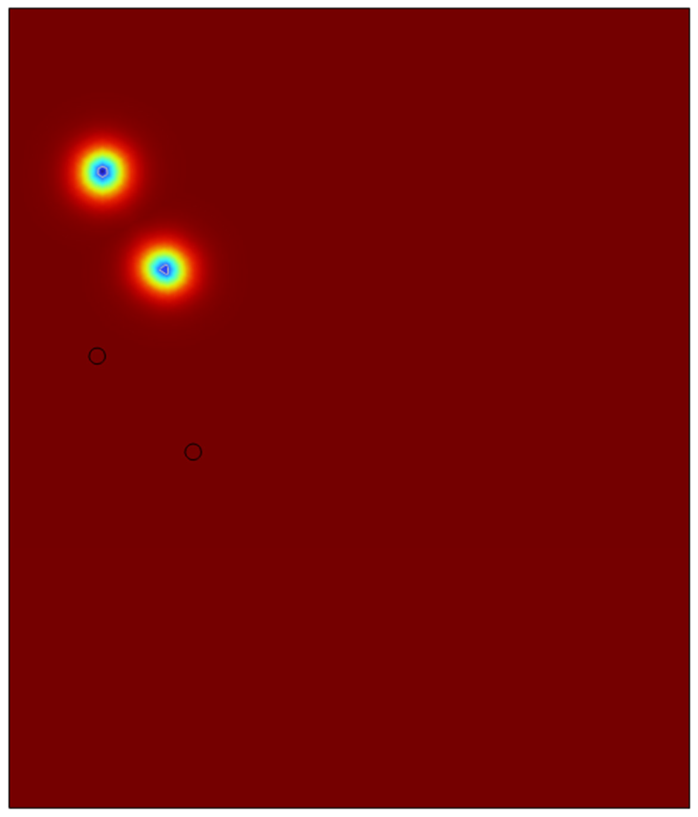
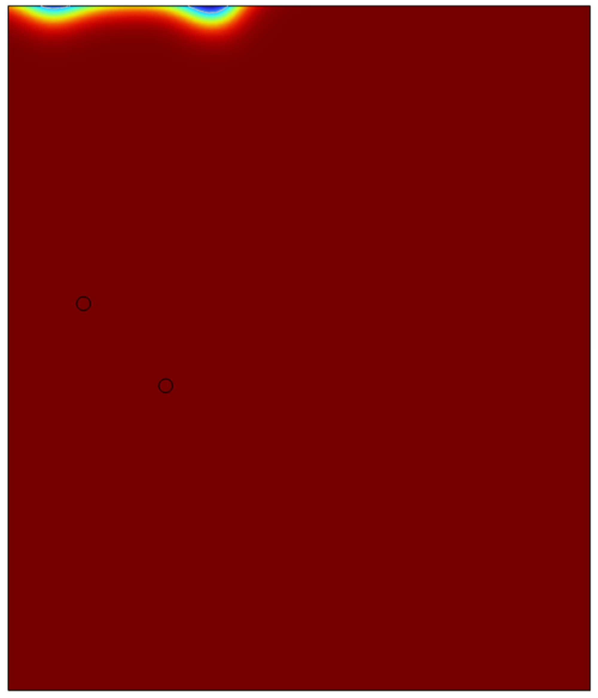
4.2. Double Microbubble System in 2-D Domain
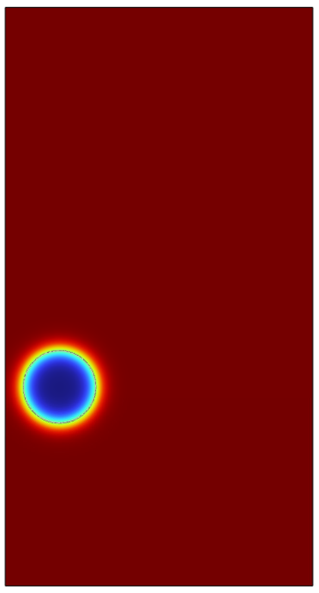
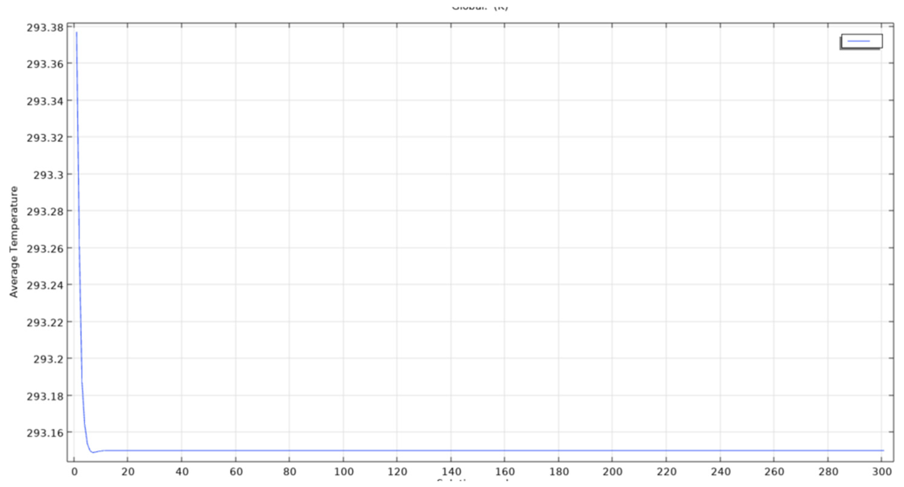
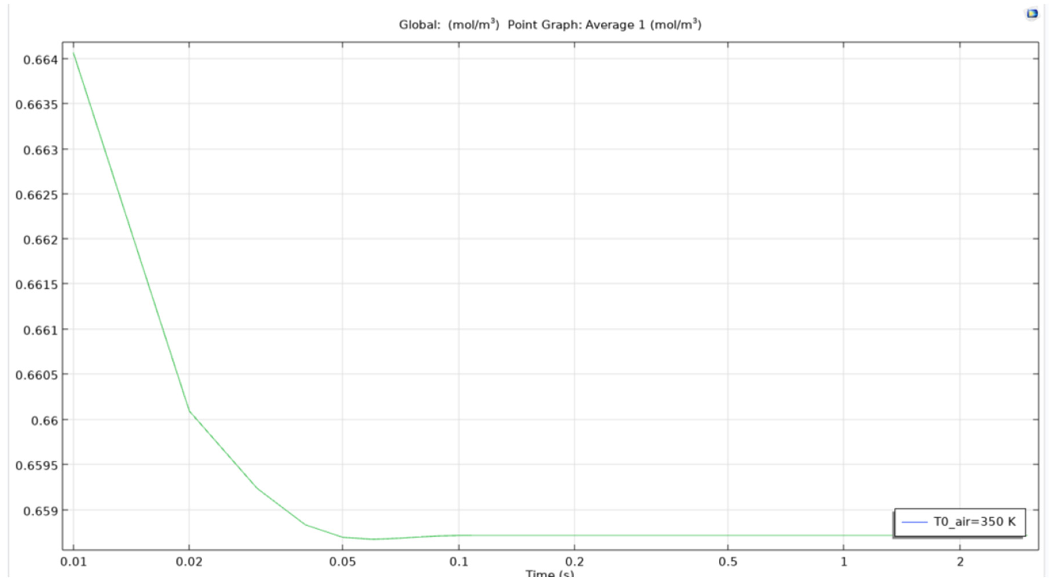
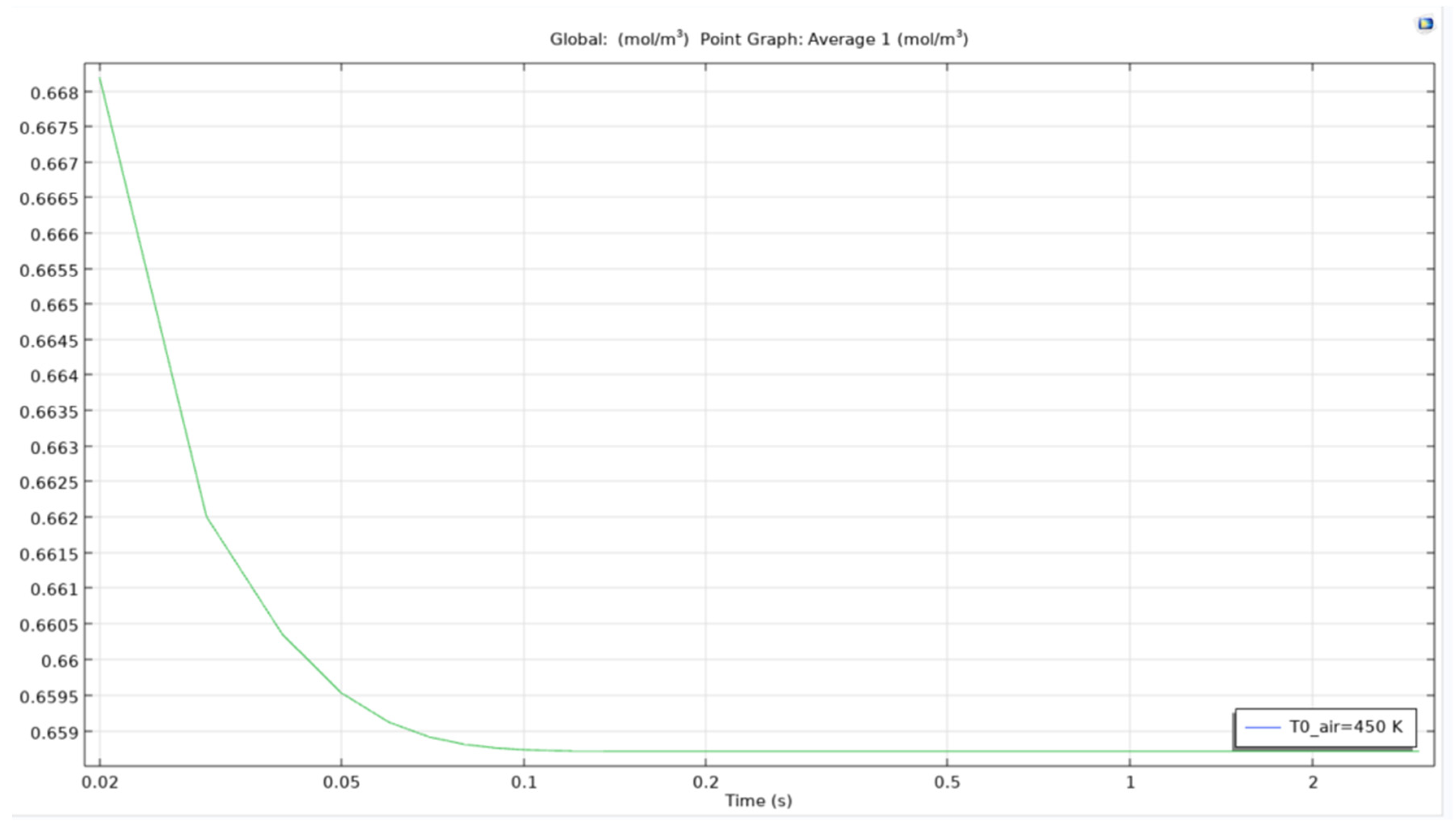
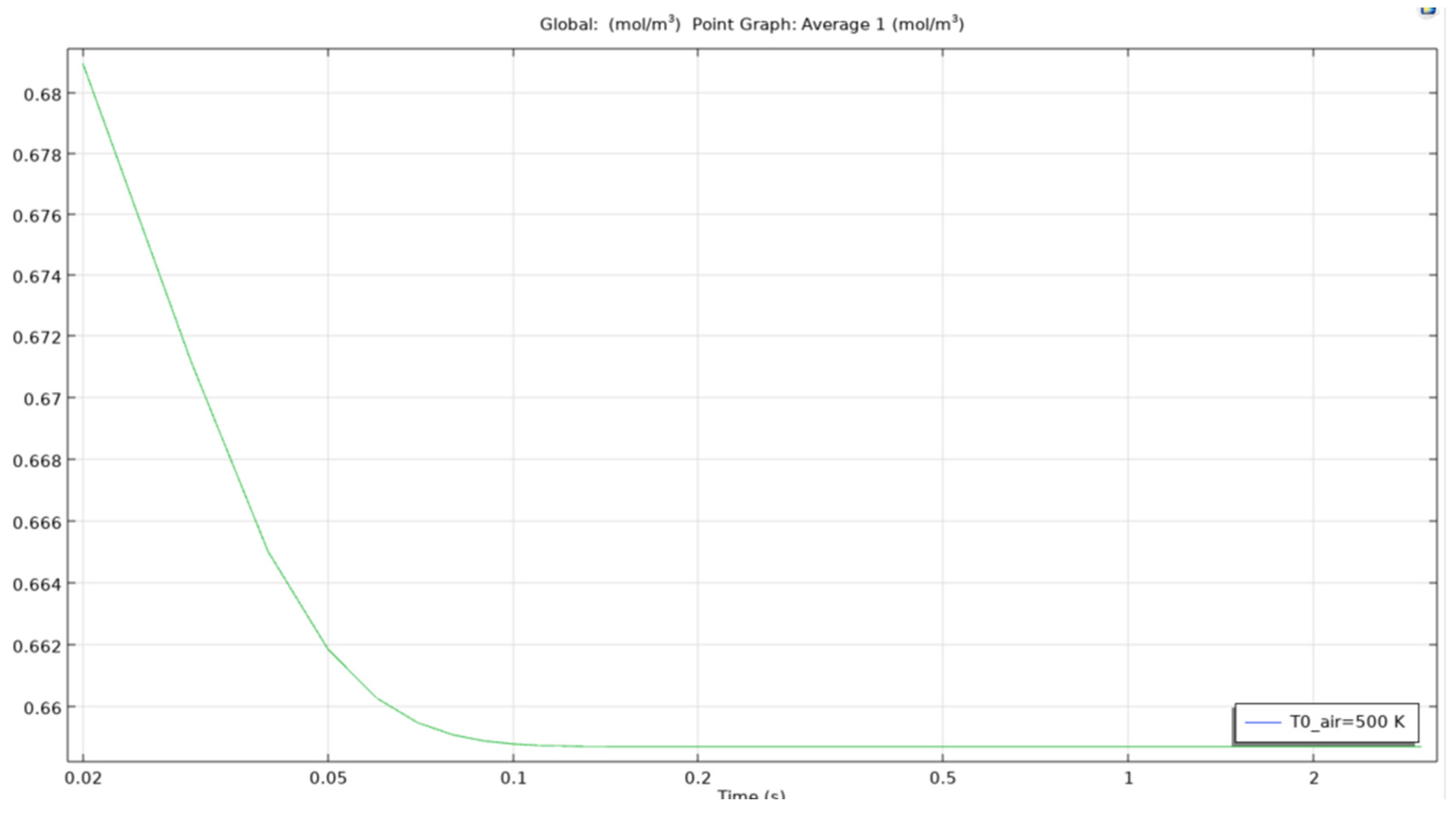
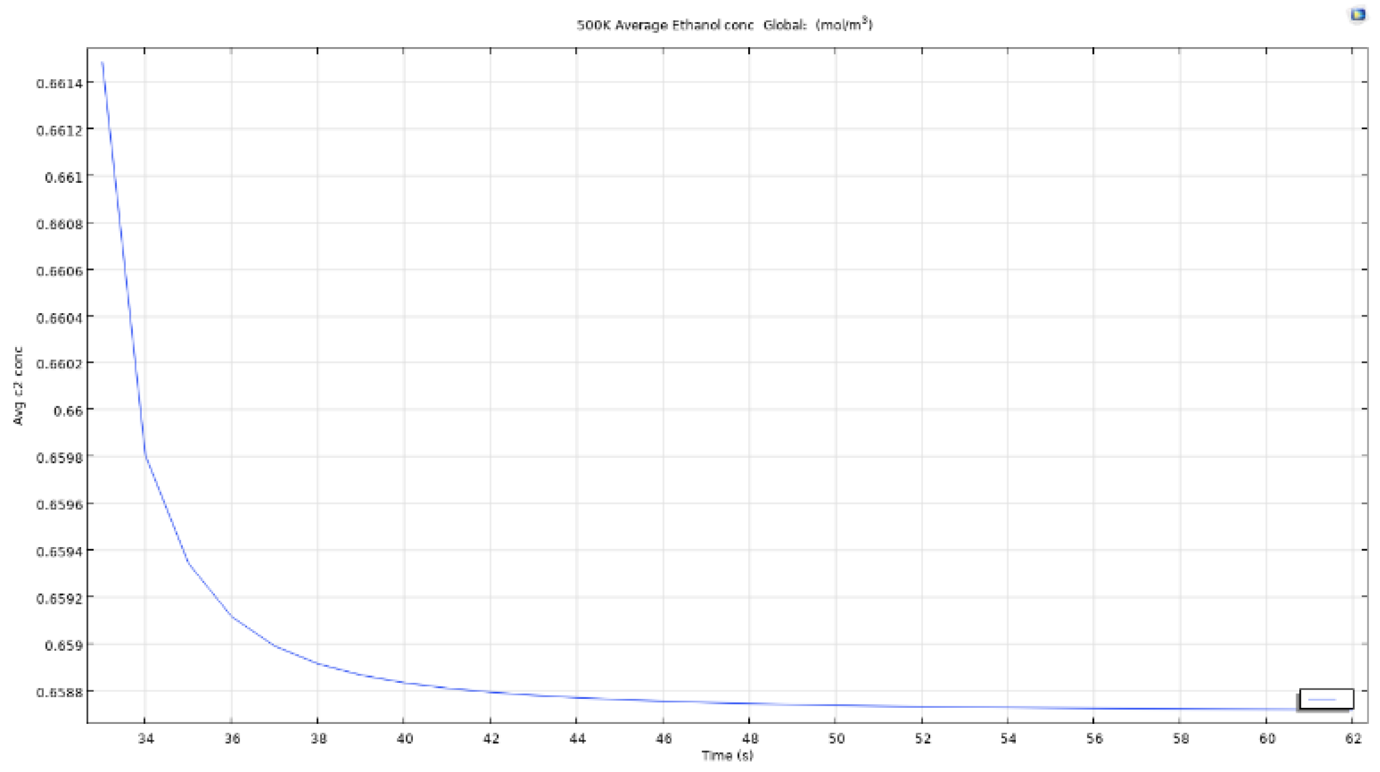
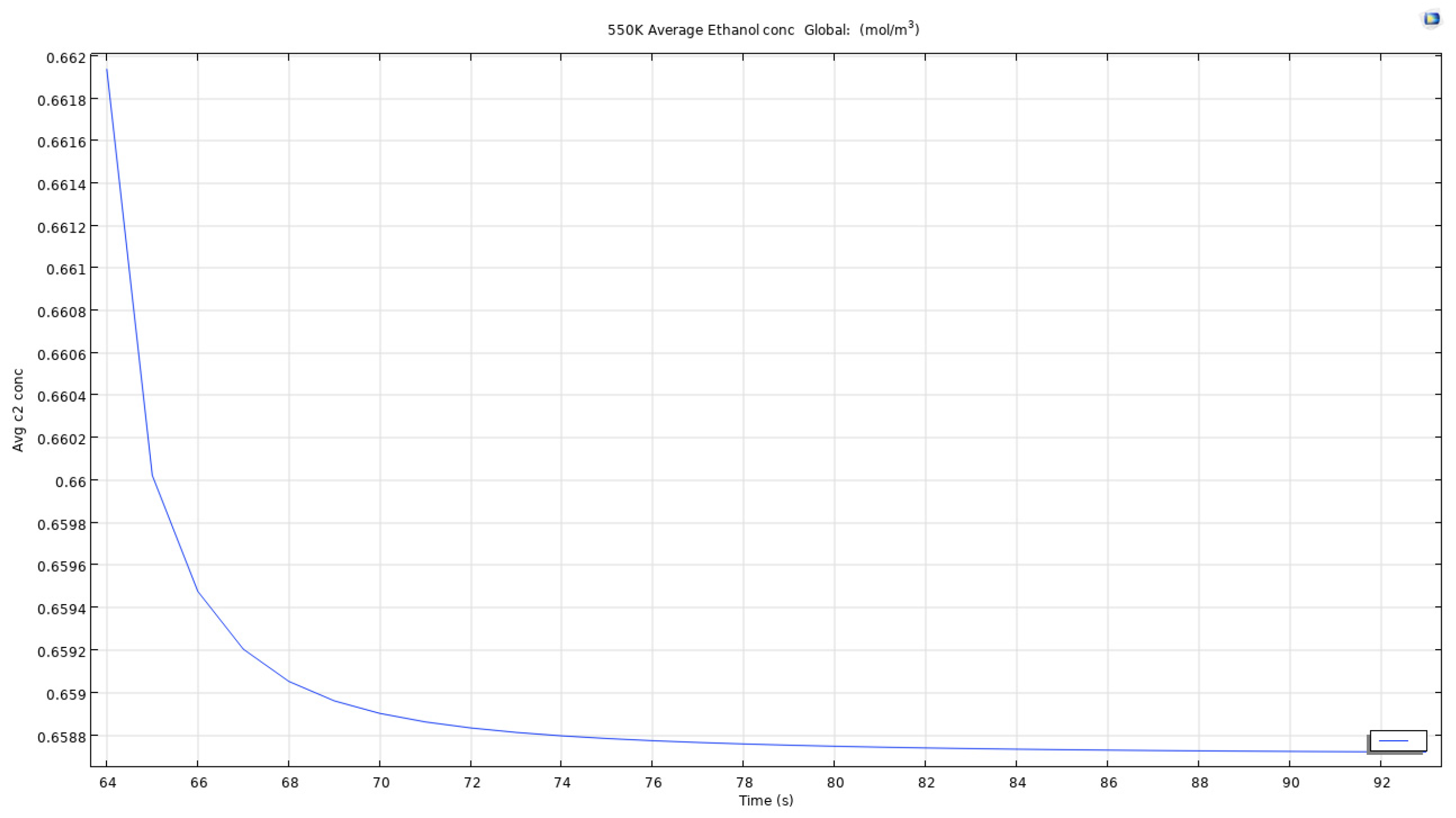
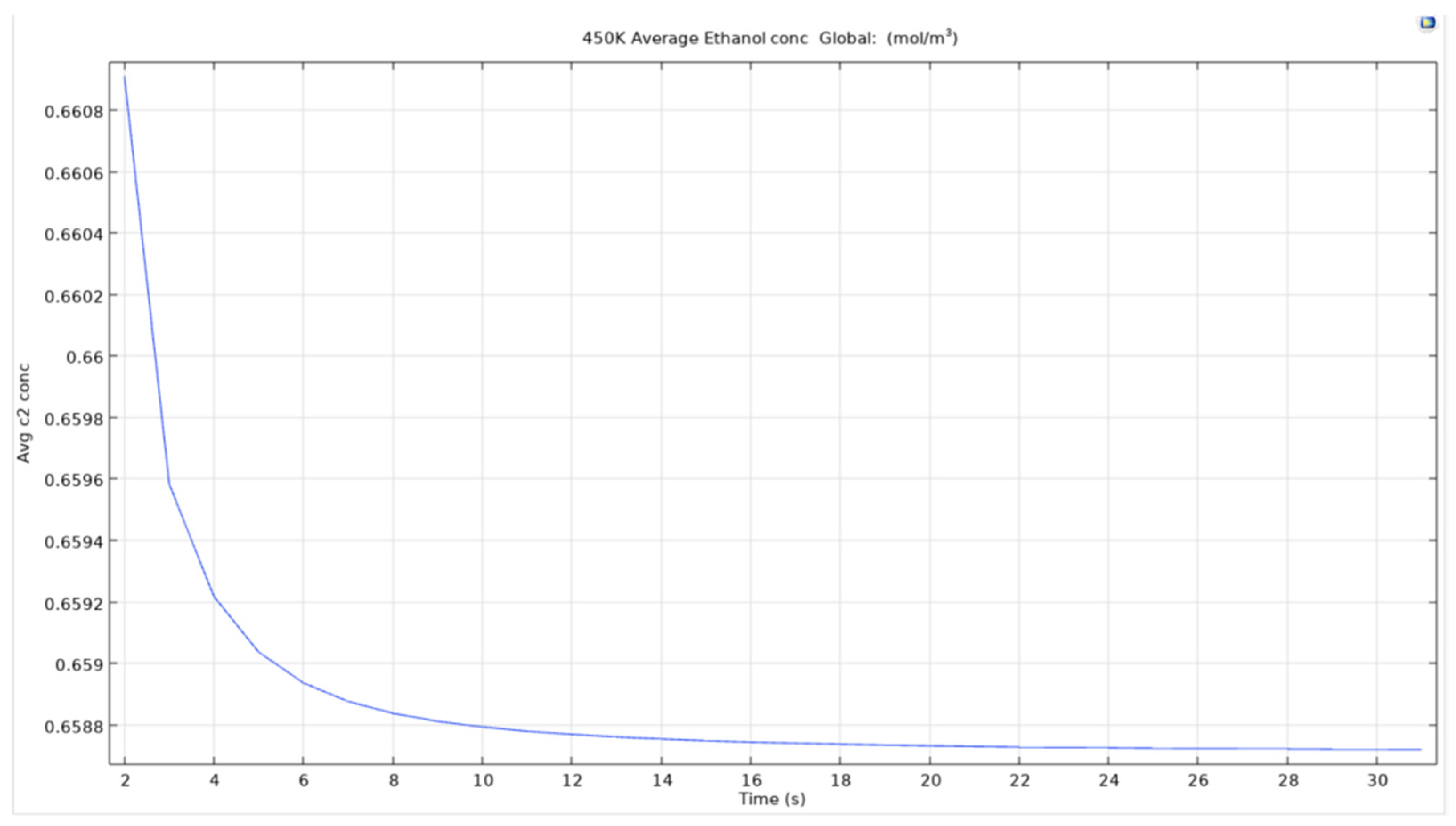
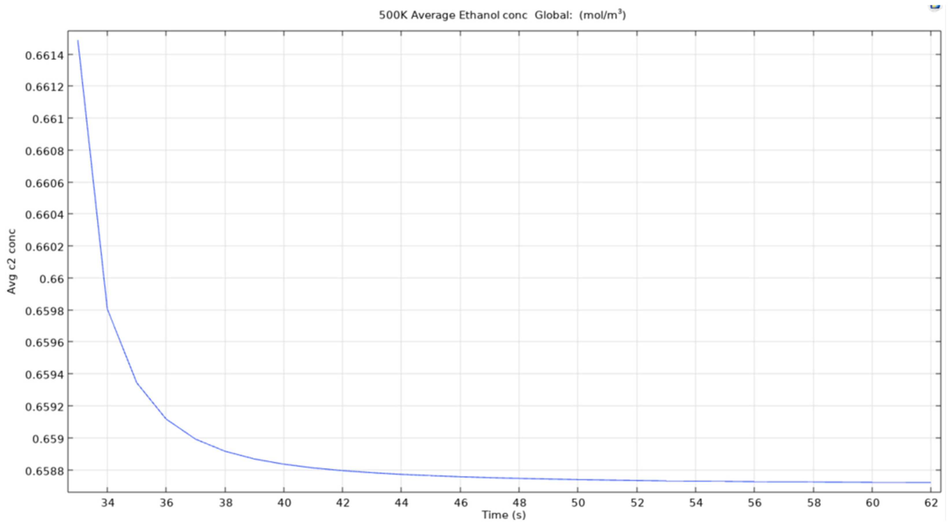
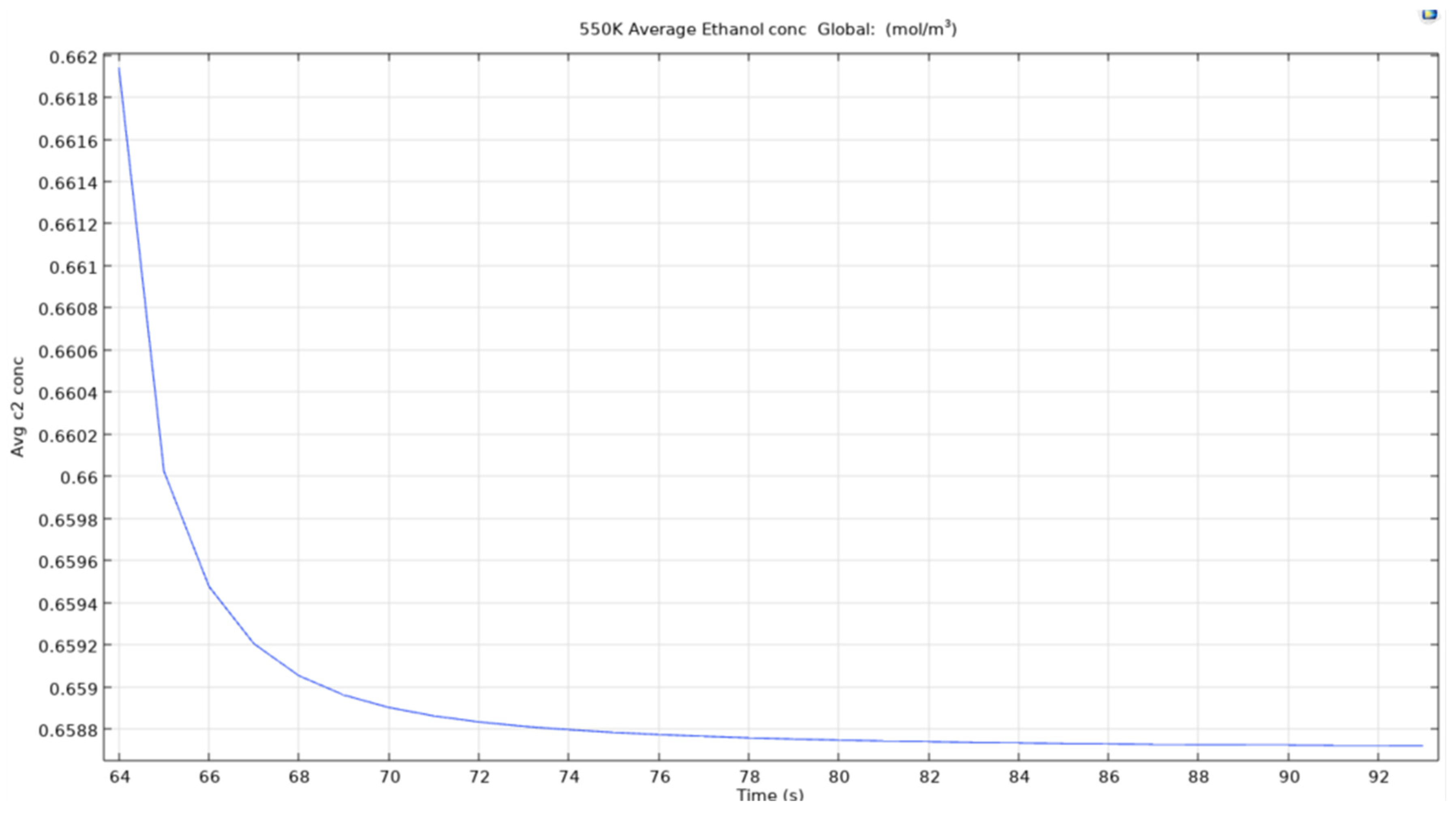
4.3. Axisymmetric Results of Original Model with Parametric Sweep
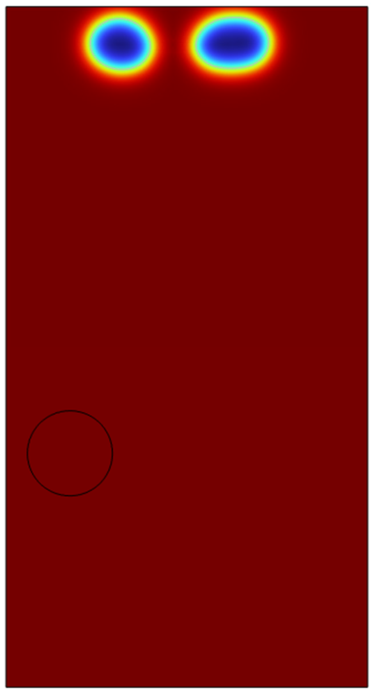
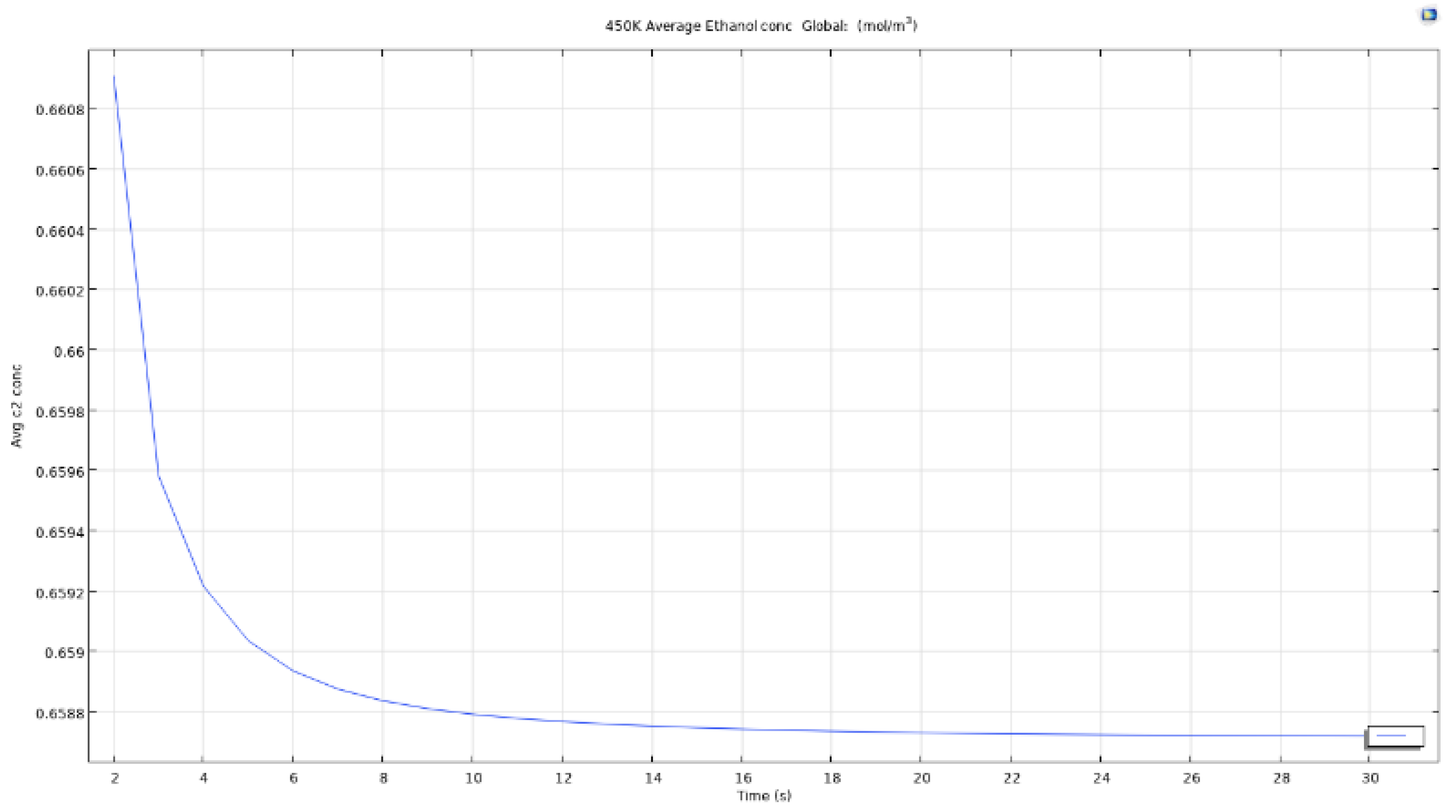
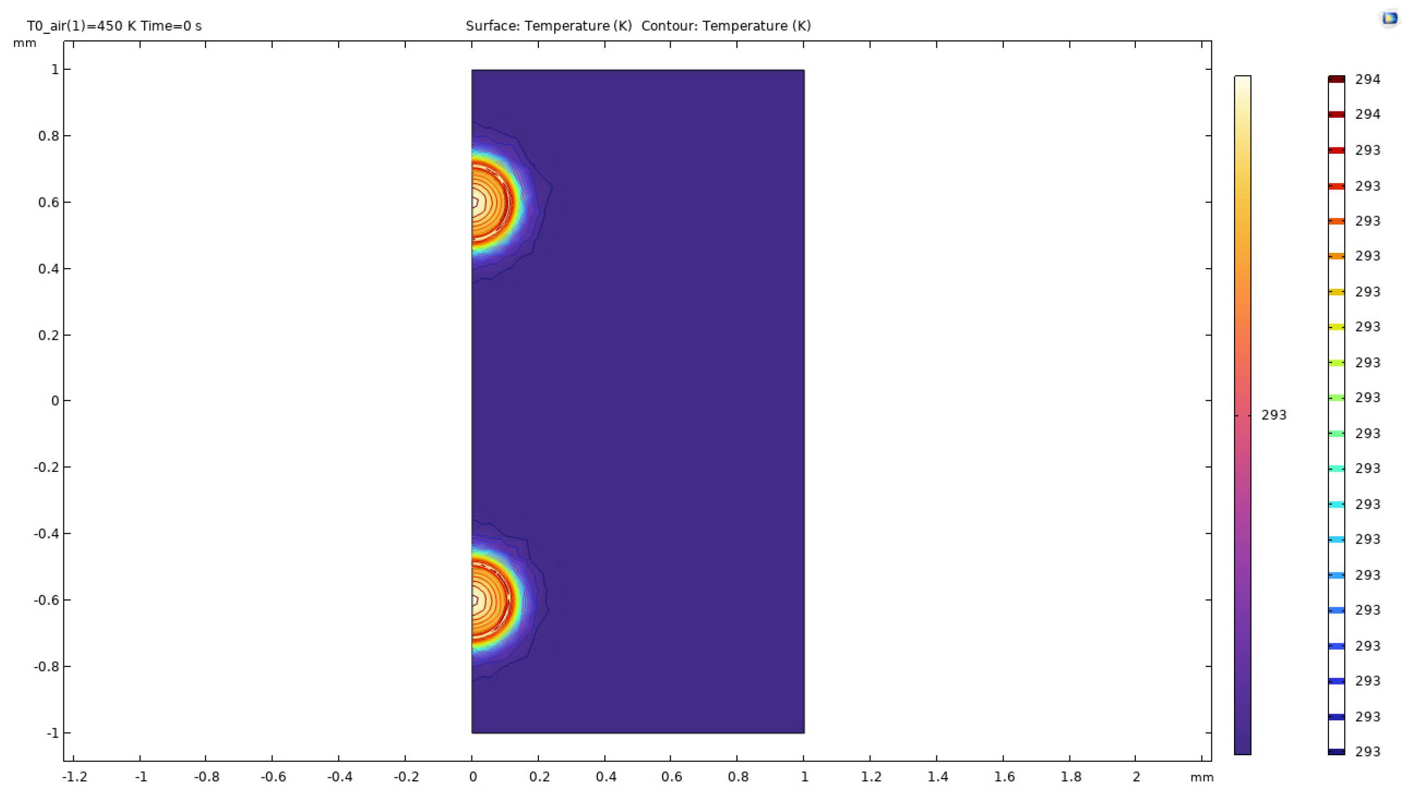
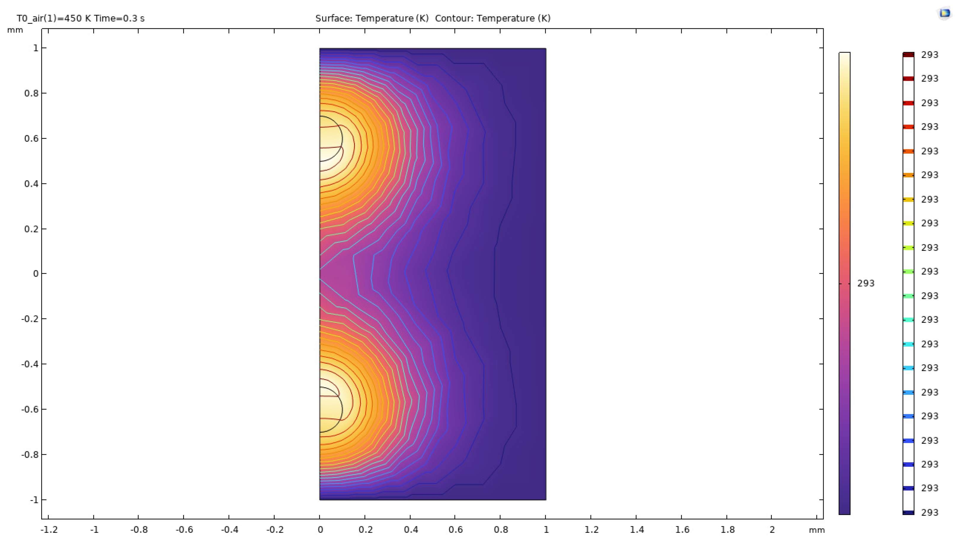
4.4. Double Bubble Axisymmetric Results
Chapter 5: Discussion
5.1. Insight
5.2. Room for Improvements- What Could’ve Been Better
Chapter 6: Conclusion and Future Work
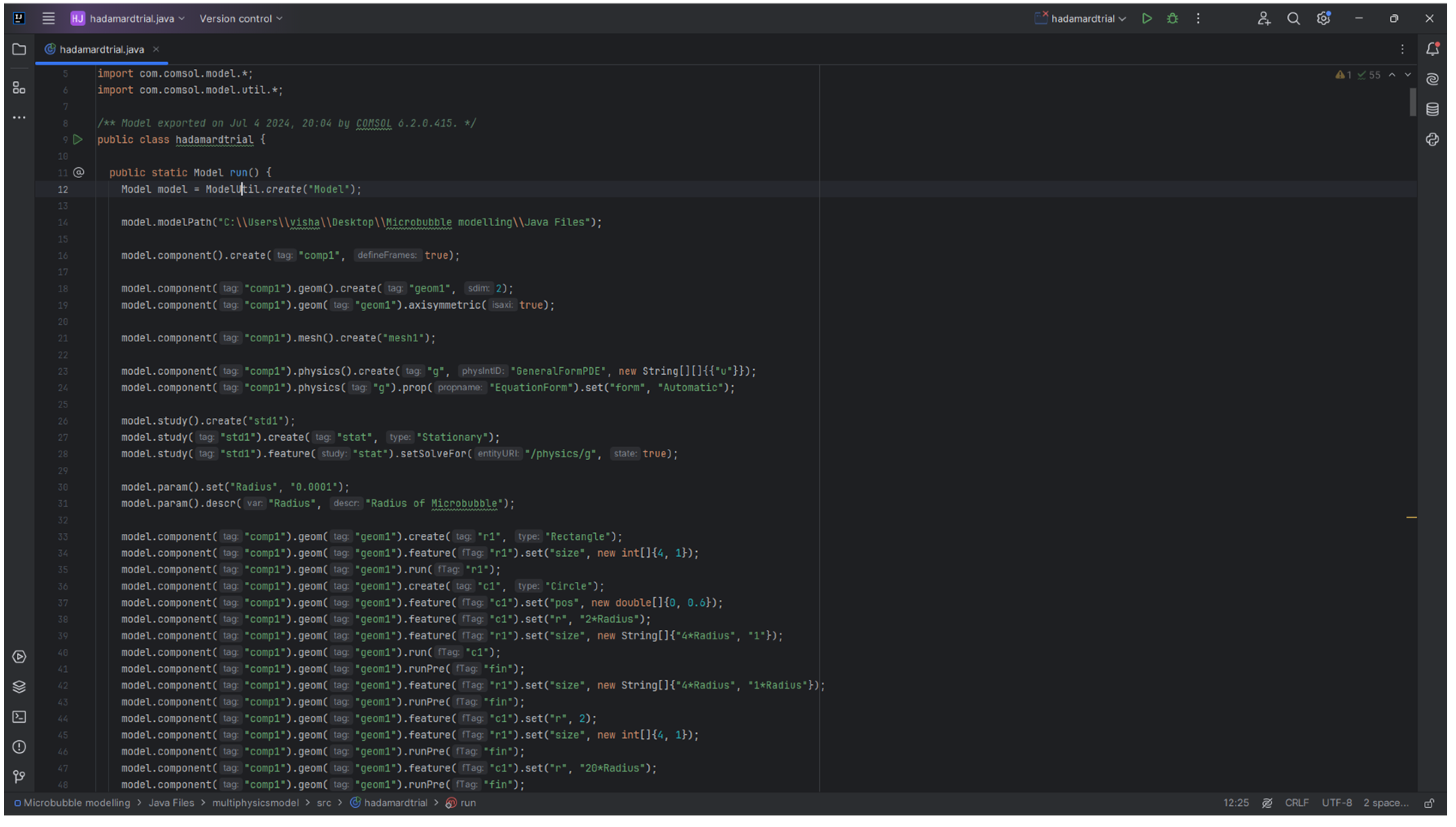
Appendix A. Java Code
|
int NUMBER_OF_BUBBLES = 1000; int ind = 0; double hx, hy, hz, hr = 0.0; double vessel_HEIGHT = 20.0; double vessel_RADIUS = 40.0; double vessel_THICKNESS = 0.2; // Set a fixed bubble radius double bubble_RADIUS = 0.1; model.component("comp1").geom("geom1").lengthUnit("mm"); model.component("comp1").geom("geom1").selection().create("csel001", "CumulativeSelection"); while (ind < NUMBER_OF_BUBBLES) { hx = (2.0*Math.random()-1.0)*vessel_RADIUS; hy = (2.0*Math.random()-1.0)*vessel_RADIUS; hz = Math.random()*vessel_HEIGHT; // Use the fixed bubble radius hr = bubble_RADIUS; if ((Math.sqrt(hx*hx+hy*hy)+hr) > vessel_RADIUS-vessel_THICKNESS) {continue; } if (((hz-hr) < vessel_THICKNESS) || ((hz+hr) > vessel_HEIGHT-vessel_THICKNESS)) {continue; } model.component("comp1").geom("geom1").create("sph001"+ind, "Sphere"); model.component("comp1").geom("geom1").feature("sph001"+ind).set("r", hr); model.component("comp1").geom("geom1").feature("sph001"+ind).set("pos", new double[]{hx, hy, hz}); model.component("comp1").geom("geom1").feature("sph001"+ind).set("contributeto", "csel001"); ind++; } model.component("comp1").geom("geom1").create("cyl001", "Cylinder"); model.component("comp1").geom("geom1").feature("cyl001").set("r", vessel_RADIUS); model.component("comp1").geom("geom1").feature("cyl001").set("h", vessel_HEIGHT); model.component("comp1").geom("geom1").create("dif001", "Difference"); model.component("comp1").geom("geom1").feature("dif001").selection("input").set("cyl001"); model.component("comp1").geom("geom1").feature("dif001").selection("input2").named("csel001"); model.component("comp1").geom("geom1").run(); |
References
- Sarkar, N., Ghosh, S.K., Bannerjee, S. and Aikat, K. (2012). Bioethanol production from agricultural wastes: An overview. Renewable Energy, 37(1), pp.19–27. [CrossRef]
- Economic Times (2024). Outlets retailing E20 fuel will cover entire country by 2025: Hardeep Puri. The Economic Times. [online] 4 Jan. Available online: https://economictimes.indiatimes.com/industry/renewables/outlets-retailing-e20-fuel-will-cover-entire-country-by-2025-hardeep-puri/articleshow/106535405.cms (accessed on 15 June 2024).
- Li, J. and Cheng, W. (2020) ‘Comparison of life-cycle energy consumption, carbon emissions and economic costs of coal to ethanol and bioethanol,’ Applied Energy, 277, p. 115574. [CrossRef]
- Vohra, M., Manwar, J., Manmode, R., Padgilwar, S. and Patil, S. (2014). Bioethanol production: Feedstock and current technologies. Journal of Environmental Chemical Engineering, 2(1), pp.573–584. [CrossRef]
- Raghavendran, V., Webb, J.P., Cartron, M.L., Springthorpe, V., Larson, T.R., Hines, M., Mohammed, H., Zimmerman, W.B., Poole, R.K. and Green, J. (2020). A microbubble-sparged yeast propagation–fermentation process for bioethanol production. Biotechnology for Biofuels, 13(1). [CrossRef]
- Aditiya, H.B., Mahlia, T.M.I., Chong, W.T., Nur, H. and Sebayang, A.H. (2016). Second generation bioethanol production: A critical review. Renewable and Sustainable Energy Reviews, [online] 66, pp.631–653. [CrossRef]
- Zimmerman, W., Tesar, V., Butler, S. and Bandulasena, H. (2008). Microbubble Generation. Recent Patents on Engineering, 2(1), pp.1–8. [CrossRef]
- Al-yaqoobi, A., Hogg, D. and Zimmerman, W.B. (2016). Microbubble Distillation for Ethanol-Water Separation. International Journal of Chemical Engineering, [online] 2016, pp.1–10. [CrossRef]
- Zimmerman, W.B. (2022). Mediating heat transport by microbubble dispersions: The role of dissolved gases and phase change dynamics. Applied thermal engineering, 213, pp.118720–118720. [CrossRef]
- Abdulrazzaq, N., Al-Sabbagh, B., Rees, J.M. and Zimmerman, W.B. (2015). Separation of azeotropic mixtures using air microbubbles generated by fluidic oscillation. AIChE Journal, 62(4), pp.1192–1199. [CrossRef]
- Abdulrazzaq, N.N., Al-Sabbagh, B.H., Rees, J.M. and Zimmerman, W.B. (2016). Purification of Bioethanol Using Microbubbles Generated by Fluidic Oscillation: A Dynamical Evaporation Model. Industrial & Engineering Chemistry Research, 55(50), pp.12909–12918. [CrossRef]
- Zimmerman, W.B., Al-Mashhadani, M.K.H. and Bandulasena, H.C.H. (2013). Evaporation dynamics of microbubbles. Chemical Engineering Science, 101, pp.865–877. [CrossRef]
- Calverley, J. (2022). Hot microbubble gas stripping for bioethanol recovery. [online] repository.lboro.ac.uk. Available online: https://repository.lboro.ac.uk/articles/thesis/Hot_microbubble_gas_stripping_for_bioethanol_recovery/20186372?backTo=/collections/Carbon_Emissions/6936102 (accessed on 16 June 2024).
- Zimmerman, W.B. (2006). Multiphysics Modelling with Finite Element Methods.
- Simulation, P. (n.d.). Easy to Use Multi-Physics Simulation Toolbox | FEATool Multiphysics. [online] www.featool.com. Available online: https://www.featool.com/multiphysics/#:~:text=Multiphysics%20is%20commonly%20referred%20to (accessed on 16 June 2024).
- Peksen, M. (2018). Multiphysics Modeling: Materials, Components, and Systems. [online] Google Books. Academic Press. Available online: https://books.google.co.uk/books?hl=en&lr=&id=vOJgDwAAQBAJ&oi=fnd&pg=PP1&dq=who+introduced+multiphysics+modeling&ots=0UsItl7xsH&sig=_wJLY78ognjXVMFZ7IR5gYPOuWw&redir_esc=y#v=onepage&q=who%20introduced%20multiphysics%20modeling&f=false (accessed on 16 June 2024).
- MPH Documentation (n.d.). MPh 1.2.4. [online] mph.readthedocs.io. Available online: https://mph.readthedocs.io/en/1.2/ (accessed on 16 June 2024).
- SimFlow (n.d.). OpenFOAM GUI - SimFlow CFD. [online] SimFlow. Available online: https://sim-flow.com/openfoam-gui/ (accessed on 16 June 2024).
- MPh Demonstrations (n.d.). Demonstrations - MPh 1.2.4. [online] mph.readthedocs.io. Available online: https://mph.readthedocs.io/en/stable/demonstrations.html (accessed on 16 June 2024).
- Kanagasabai, M., Maruthai, K. and Thangavelu, V. (2019). Simultaneous Saccharification and Fermentation and Factors Influencing Ethanol Production in SSF Process. [online] www.intechopen.com. IntechOpen. Available online: https://www.intechopen.com/chapters/67972.
- Brittle, S., Desai, P., Ng, W.C., Dunbar, A., Howell, R., Tesař, V. and Zimmerman, W.B. (2015). Minimising microbubble size through oscillation frequency control. Chemical Engineering Research and Design, 104, pp.357–366. [CrossRef]
- Constantin, O. (2010). Fluidic Elements based on Coanda Effect. INCAS BULLETIN, 2(4), pp.163–172. [CrossRef]
- Barve, D. (2024). ISMA predicts major surplus for sugar production in FY23-24 - Agro Spectrum India. [online] Agro Spectrum India. Available online: https://agrospectrumindia.com/2024/07/03/isma-predicts-major-surplus-for-sugar-production-in-fy23-24.
- Barve, D. (2024). ISMA predicts major surplus for sugar production in FY23-24 - Agro Spectrum India. [online] Agro Spectrum India. Available online: https://agrospectrumindia.com/2024/07/03/isma-predicts-major-surplus-for-sugar-production-in-fy23-24.html#:~:text=The%20Indian%20Sugar%20and%20Bio (accessed on 2 September 2024).
- W3schools.com. (2024). W3Schools.com. [online]. Available online: https://www.w3schools.com/java/java_encapsulation.asp#:~:text=The%20get%20method%20returns%20the%20variable%20value%2C%20and (accessed on 2 September 2024).
- Abdulrazzaq, N. (2017). Application of Microbubbles Generated by Fluidic Oscillation in the Upgrading of Bio Fuels - White Rose eTheses Online. Whiterose.ac.uk. [online]. Available online: https://etheses.whiterose.ac.uk/16491/1/nnabdulrazzaqphdthesis.pdf.
- The Wire. (2024). Modi Govt’s Decision to Hike Sugarcane Prices Offers Little to Distressed Farmers. [online]. Available online: https://thewire.in/government/sugarcane-price-hike-frp-modi-govt (accessed on 2 September 2024).
- COMSOL. (2017b). How to Create a Randomized Geometry Using Model Methods. [online]. Available online: https://www.comsol.com/blogs/how-to-create-a-randomized-geometry-using-model-methods/?cv=1 (accessed on 2 September 2024).
Disclaimer/Publisher’s Note: The statements, opinions and data contained in all publications are solely those of the individual author(s) and contributor(s) and not of MDPI and/or the editor(s). MDPI and/or the editor(s) disclaim responsibility for any injury to people or property resulting from any ideas, methods, instructions or products referred to in the content. |
© 2024 by the authors. Licensee MDPI, Basel, Switzerland. This article is an open access article distributed under the terms and conditions of the Creative Commons Attribution (CC BY) license (http://creativecommons.org/licenses/by/4.0/).


