
Submitted:
12 November 2024
Posted:
20 November 2024
You are already at the latest version
Abstract
There is no question that photovoltaics are a mainstream technology fundamental to achieving carbon neutrality. In this context, we analyzed and compared the outdoor performance of PERC (Passivated Emitter and Rear Contact) solar modules with modules using the recent HJT (Heterojunction Technology). After discounting the measurement error sources in our experimental tests, we concluded that HJT technology was, on average, 1.88\% more efficient than PERC technology. However, this number alone is not sufficient. Despite this indication, different PV system scenarios were also simulated to answer the right question: is there any “optimal” scenario with characteristics more favorable to some or even both of these technologies? Based on these simulated scenarios, which used the parameters identified in our experimental tests, we concluded that in cases of constraints related to the installed power or limited area, HJT modules should be installed. These will be capable of returning more profit in the long run despite both technologies becoming profitable in the short term. In cases with a limited budget, PERC modules should be installed, as they will be a better investment regardless of the time considered for the analysis.
Keywords:
Passivated Emitter and Rear Contact
; Heterojunction Technology
; PERC
; HJT
; Photovoltaic
1. Introduction
The performance of a photovoltaic (PV) module is strongly dependent on ambient conditions (e.g., irradiation, ambient temperature, wind), which cause different power losses occurring in the solar cells. These losses are related to the increased cell temperature and are associated with the recombination effect. Therefore, each electron-hole pair that is not collected reduces the cell efficiency.
Several technologies were improved in the past century and are currently used to lower the recombination losses and the temperature coefficient. In 2020, 85% of the market share was occupied by the passivated emitter and rear contact (PERC) technology [1] due to the low cost of manufacture and high efficiency. However, this photovoltaic cell displays a high-temperature coefficient and light-induced degradation (LID). As usual, the market is constantly looking for improvements in the technology used. Interest then has risen around the heterojunction (HJT) cell due to its lower temperature coefficient, lower recombination rates, and natural bi-facial nature.
1.1. PERC—Passivated Emitter and Rear Contact
From an optical perspective, the power output is directly related to the amount of incident light absorbed by the cell. Silicon nitride acts as an anti-reflection coating, allowing more light to penetrate the cell, resulting in superior efficiency.
Defects at the silicon surface are caused by the interruption of the crystal lattice periodicity, and, as a result, unpaired electrons appear. These are called dangling bonds and generate a high local recombination rate.
Minimizing surface recombination, i.e., passivation, is thus a prerequisite for achieving high-efficiency cells. This is achieved by combining two effective mechanisms: chemical passivation by intrinsic hydrogen and field-effect passivation via fixed insulator charges [2]. Due to the high refractive index and the superior surface passivation, silicon nitride layers are applied in silicon solar cells.
1.1.1. Al2O3-Based Rear Surface Passivation Scheme
Rear surface passivation was improved by introducing aluminum oxide as a charged dielectric. This innovation became the basic element of the industrial PERC (Passivated Emitter and Rear Contact) device.
Fixed negative charges present in the Al2O3 film attracting holes to form an accumulation layer on p-type silicon [4], being this effect illustrated in Figure 1. This positively charged layer results in a recombination decrease [3]. Also, the flow of electrons along the rear surface in the direction of the highly recombinative base contacts is suppressed. Due to these advantages, has a high potential for increasing solar cell efficiency [5].
subsubsection Al2O3 / SiNx- Stacks for PERC Solar Cells When incident light is not absorbed, it reaches the back structure that supports the module, and energy is converted into heat, raising cell temperature and decreasing efficiency.
The combination of aluminum oxide and silicon nitrite provides passivation and creates a mirroring effect for incident light [6], enhancing its absorption within the solar cell. For these two mentioned reasons, combining these two layers on the back of the cell is fundamental to boosting the efficiency of photovoltaic cells. With a layer of silicon nitride on the front, the PERC cell is completed and displayed in Figure 2.
Although some improvements were made and higher efficiency was achieved, this technology still presents light-induced degradation.
1.1.2. LID—Light-Induced Degradation
Besides challenges in process technology, stability issues due to light-induced degradation have been a critical challenge for highly efficient p-type solar cells. This LID can happen due to the boron-oxygen (BO) effect and Light and elevated Temperature-Induced Degradation (LeTID).
Under the light exposition effect, may diffuse across the silicon lattice and create complexes with boron acceptors. The boron-oxygen complexes create energy levels in the silicon lattice and can capture electrons and holes, which are lost for the PV effect. This effect happens when the panel is first exposed to sunlight, resulting in an instant decrease in efficiency, as seen in Figure 3.
The second process, as the name indicates, relates severe efficiency degradation with high temperature and, if not controlled, can lead to losses of more than . Engineers have been trying to solve these inefficiency issues, and a solution was found. In contrast to conventional PERC, Hanwha Q CELLS’ Q.ANTUM technology reliably suppresses both LID due to BO defect formation and LeTID in modules manufactured [7].
It is possible to conclude that, with the insertion of a silicon nitride anti-reflection coating on the front of the cell, the creation of passivation and a mirroring effect on the back, and the solution of LID-related inefficiencies, PERC is one of today’s market competitors for high-efficiency mass production cells.
1.2. SHJ—Silicon Heterojunction Cell
As discussed in the previous paragraphs, high-efficiency solar cells can be obtained by implementing surface passivation layers that severely reduce recombination losses. This is achieved by the implementation of dielectric layers such as Silicon nitride (), Silicon Oxide (), aluminum oxide () or intrinsic hydrogenated amorphous silicon.
The first three layers have already been described since some are applied to PERC cells. invented heterojunction intrinsic thin-layer solar cells (HIT) technology in the early 1990s and benefited from using intrinsic hydrogenated amorphous silicon layers for higher efficiency. The concept of a diode using a heterojunction formed by amorphous silicon layers and crystalline silicon was initially proposed in 1974. However, it was only commercialized by 18 years later. The term heterojunction comes from the formation of the junction of semiconductors with different bandgaps. This is verified in the cross-sectional view of SHJn in Figure 4, where an n-type Silicon (c-Si(n)) is sandwiched between two amorphous Silicon intrinsic layers (a-Si:H(i)).
Using the amorphous layers, surface recombination is suppressed by the chemical passivation of dangling bonds on the c-Si wafer surface. This is possible due to the formation of Si-Si and Si-H bonds [9]. Amorphous silicon layers only provide passivation if they are in contact with intrinsic layers. Intrinsic means that the layers have not been doped intentionally.
Continuing the analysis of the SHJn cell, displayed on the left part of Figure 4, a p-type amorphous layer (a-Si:H(p)) is grown on the top, and on the bottom, n-type amorphous layers (a-Si:H(n)) is deposited. These layers are then fully covered with a transparent conductive oxide (TCO), followed by screen-printing contact metal grids using low-temperature Ag conductive paste. TCOs are required to enhance the collection of the electron-hole pair and are transparent to allow light to enter the cell.
Both n- and p-type doped wafers have been used for SHJ cells, but the highest efficiency was obtained for SHJn cells. It is important to note that the relation of a-Si/c-Si is roughly 1:10000. From the studies conducted on these materials, n-type wafers display lower recombination rate, lower sensitivity to metal impurities, and, unlike p-type, are not affected by LID [3]. Adding to these advantages, SHJ cell assembly is performed at low temperatures (<250°C), favoring thin wafers for cell production.
commercialized this technology under patented Heterojunction with Intrinsic thin layer (HIT). This patent expired in 2010 and opened the way for equipment suppliers and manufacturers to work with the technology and provide solutions to the market. is a Swiss company that used to manufacture machinery required to produce wafers in mass production. After 2010, they started working on the Heterojunction technology and are present today with HJT + SmartWire Connection Technology (SWCT). It consists of a small wire to replace busbars on the top and bottom grid of the cell, as seen in Figure 5. This technology can increase the efficiency of the HJT cell by 5,7% due to the reduced electrical losses and optical losses (less shading) due to the reduced size compared to the bus bar technology [10].
2. Experimental Set-Up
2.1. PERC Modules
The mono-crystalline 395W panels with reference JAM54S31/MR/1000V from JASOLAR were chosen to study the PERC technology. These panels present a half-cell configuration, meaning that instead of having one circuit, the panel is divided into two parallel ones, halving the current values. Regarding the Joule loss effect, where the losses are related to the square value of the current, its values drop to 1/4. There is no reference to using any LID suppression technology for this module, so it was assumed to be nonexistent.
In Figure 6, the electrical parameters at standard test conditions (STC- irradiance of 1000W/m2, cell temperature of 25°C and an air mass of 1.5) of the PV module are displayed. Note that the module displays 395W of Rated Maximum Power, corresponding to the values located far to the right in Figure 6.
2.2. HJT Modules
The mono-crystalline Glass modules were chosen to study the HJT technology. It presents a half-cell technology, meaning that the Joule loss effect is decreased to 1/4, and the panel gathers irradiance from both sides due to its natural bi-facial configuration. Figure 7 and Figure 8 display the electrical parameters at the STC of the PV panel. Table 1, the most important parameters in STC are gathered.
It is important to note that despite presenting 25 W of the rated power difference, efficiencies are very similar. Regarding the temperature coefficient, a bigger decrease in the PERC output power is expected with the increase in temperature.
2.3. Location and Connection
The HJT and PERC panels were mounted horizontally side-by-side on the Institute’s rooftop, as seen in Figure 9.
2.4. Data Acquisition
The setup displayed in Figure 12 was the acquisition system at the laboratory. The right piece was connected to the HJT module, while the left was connected to the PERC module.
A variable resistor was connected directly to the panel to achieve maximum power, as shown in Figure 12.
This resistor was chosen due to its high current support- 16A. Also, the resistance range [1, 9] is superior to the MPP resistance. For STC conditions, the HJT module displays 37,7V and 9,9A at MPP. This way, the correspondent resistance of 3,80 is obtained by Ohm’s Law . For the PERC module, MPP is characterized by 30,64V and 12,61A, corresponding to 2,41.
A power signal was obtained by visualizing the voltage, displayed in Figure 13 in yellow, and current signals, in blue, and multiplying both signals. With the oscilloscope reading the signal during a time interval of 5 seconds, the resistor values were changed from minimum to maximum. In between, the maximum power point would be visualized by searching the point of maximum amplitude on the red signal, as seen in Figure 13. Then, visualizing the correspondent current and voltage values on the yellow and blue signals, it was possible to compute the MPP. This approach was taken to collect data on the photovoltaic panels working under load conditions.
3. Results
To evaluate each module’s efficiency, the equation 1 was used.
Where:
- is the module output power, in W, computed via the oscilloscope;
- G is the horizontal irradiance, in W/m2;
- A is the module active area. The HJT module area equals 1,793m2, and PERC has an area of 1,953m2;
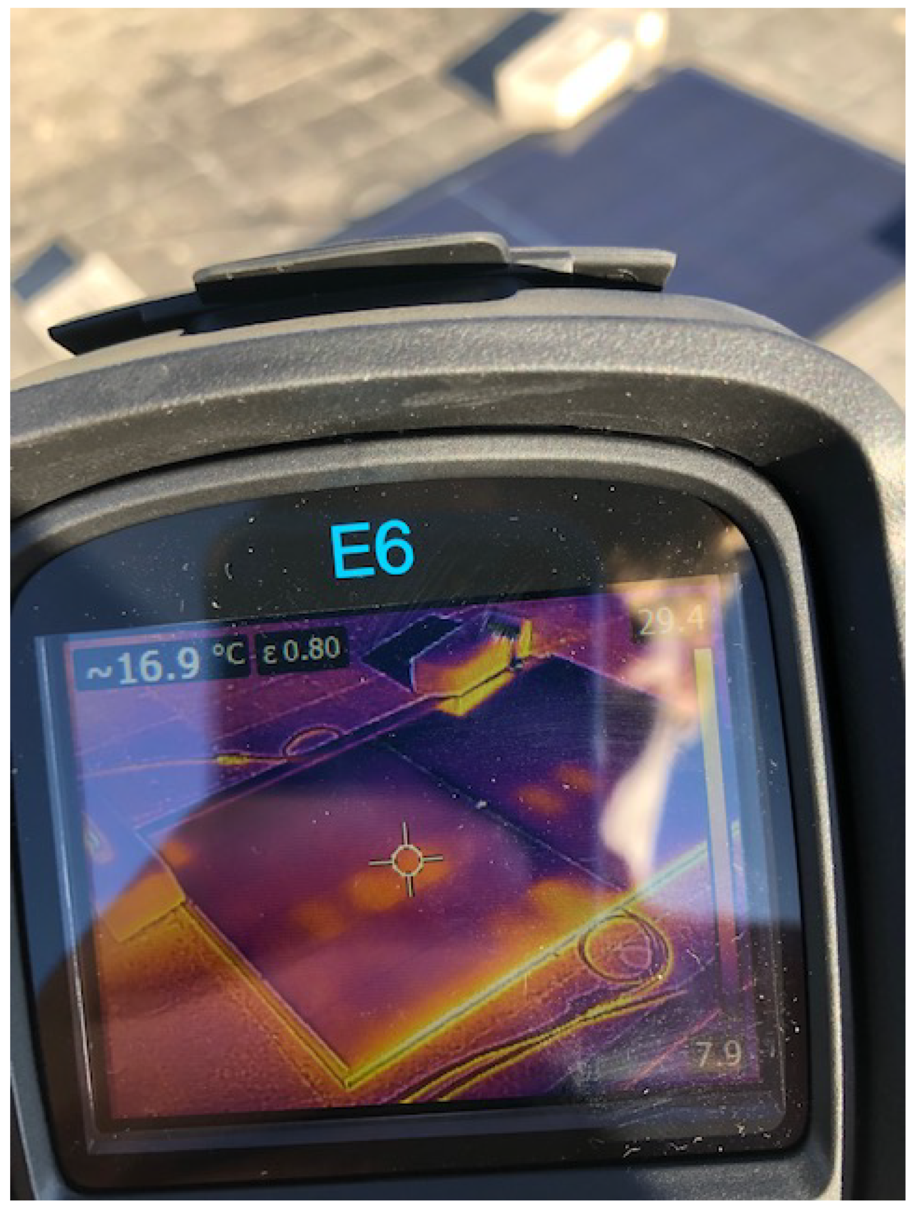
Temperature measurements are performed with infrared camera FLIR E6-XT, as shown in Figure 15, always on the same cell on each module. Horizontal irradiance measurements are performed with the Pro Solar Power Meter ISM400 shown in Figure 14.
Figure 14.
Horizontal irradiance acquisition.
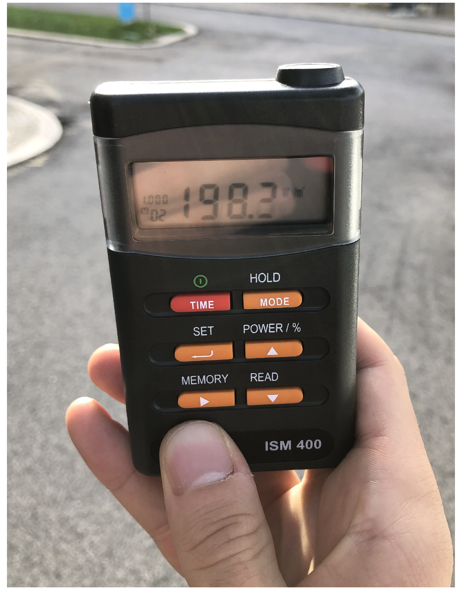
Figure 15.
Horizontal irradiance acquisition.
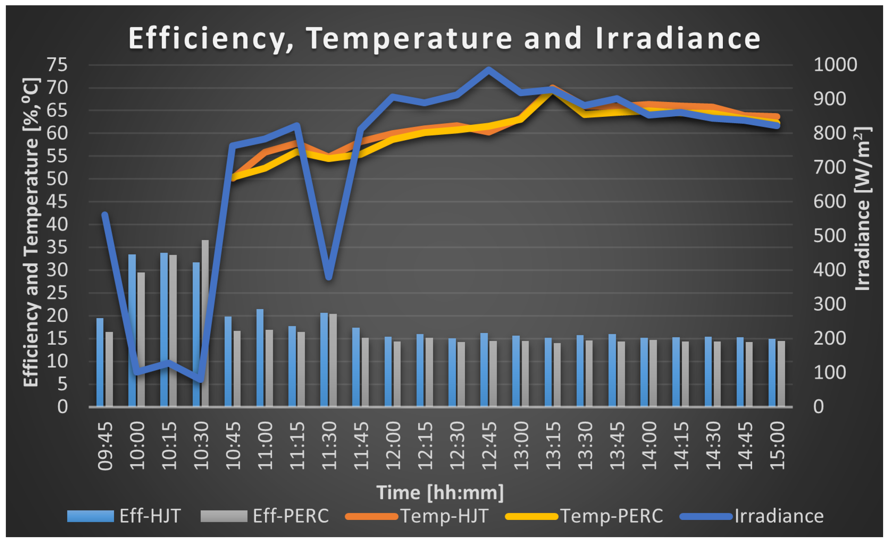
Data was collected in various weather to obtain a diversified set of samples and evaluate cell technology performance in different conditions. The purpose was to evaluate and compare the differences in performance throughout the day. The experimental results will be shown using two figures displaying the parameters for the desired day: one for module efficiency and temperature and a second for the other for module efficiency, module temperature, and now irradiance.
3.1. 18th of August—Clear Sky Conditions
All instruments were available to characterize both module performances for the data collection performed on the 18th of August and the remaining days. This way, there are irradiance, module temperature, and efficiency values. Throughout the day, no clouds appeared, and both panels received direct radiation from the sun.
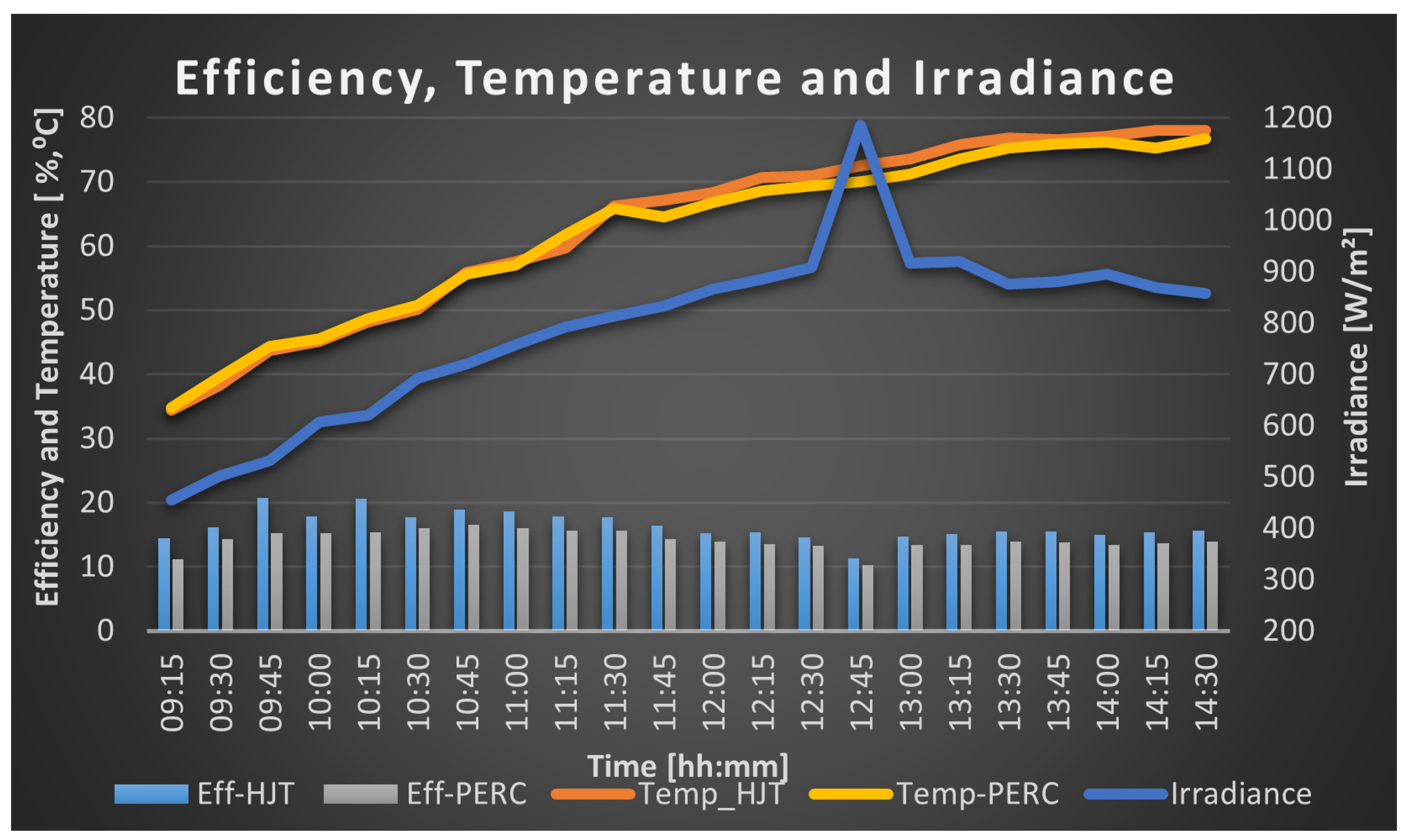
Analysing Table 2 and Figure 16 and Figure 17, it is possible to observe that the HJT panel displayed, on average, 2.37% more efficiency than PERC during this sunny summer day. Except for the value read at 12:15, between 08:30 and 13:00, the irradiance kept increasing. It was expected to visualize an increasing trajectory in efficiency during this time interval, but panel temperature increased as well. It can be seen that maximum efficiency, 21.91%, was obtained for the HJT panel at 10:15 with a module temperature of 42.1°C and irradiance of 602 W/m2. For the PERC panel, however, a maximum efficiency of 17.19% was achieved at 10:45 with a module temperature of 52°C and irradiance of 677 W/m2.
Figure 16.
Module efficiency and temperature for August’s 18th.
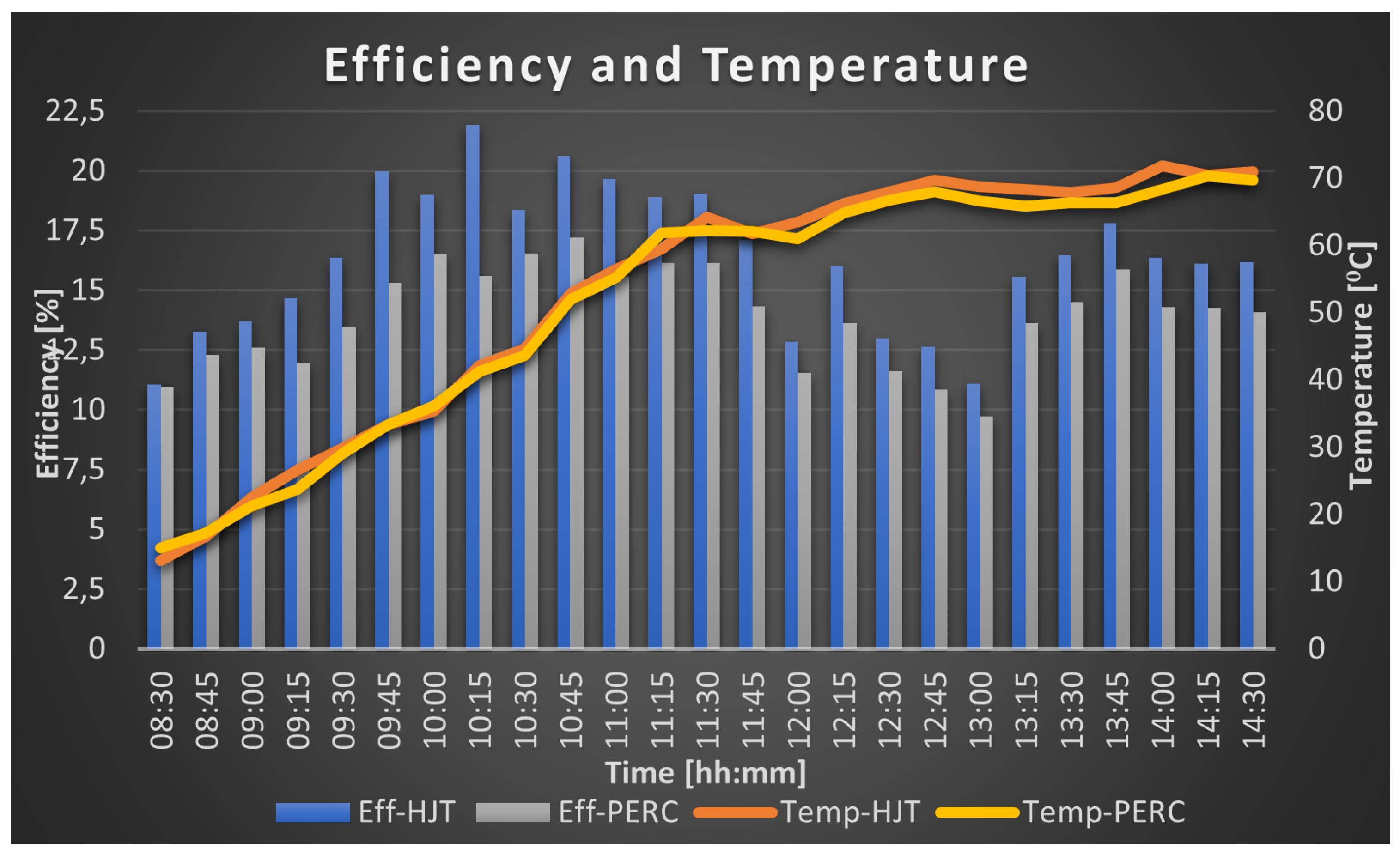
Figure 17.
Irradiance, module efficiency, and module temperature for August’s 18th.
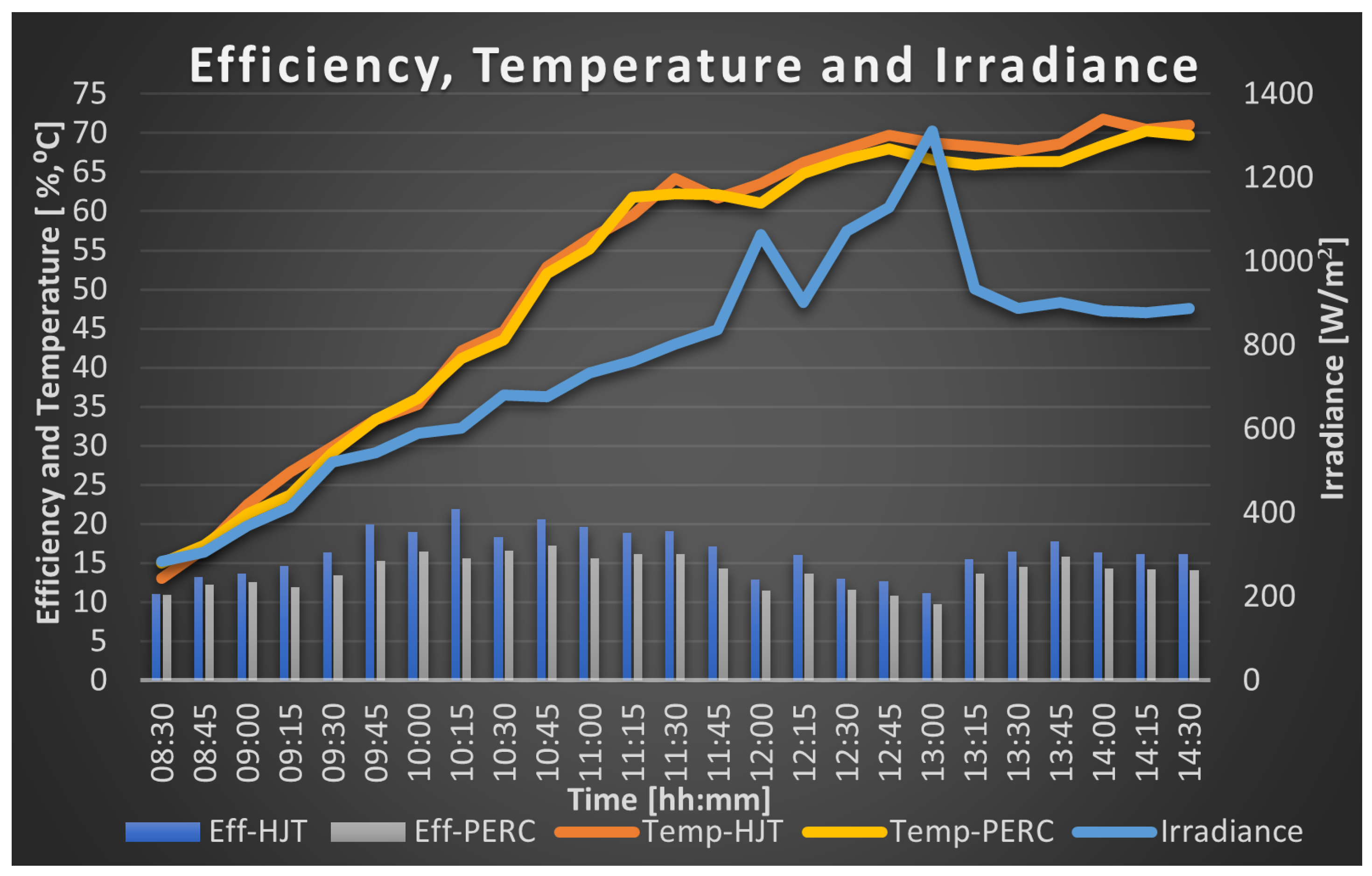
How the temperature affects module output is noticeable after both modules present a temperature above the [50°C; 60°C] range. Despite the continuous increase in irradiance, efficiency values drop to 11.10% and 9.70% on HJT and PERC, respectively, at 13:00. This behavior reflects the difficulty that solar cells generally present while working under high module temperatures.
Between 12:15 and 14:30, both modules presented temperatures above 64°C. It would have been expected that even though both panels display very high working temperatures, an increase in irradiance would reflect an increase in efficiency. This was not verified. For high operating temperatures, an increase in irradiance results in an efficiency decrease, noticeable in both technologies for the period between 12:15 and 13:00. When irradiance values drop from 1312 W/m2 at 13:00 to 935.2 W/m2 at 13:15, a noticeable increase of approximately 4% in each module efficiency was then observed.
When irradiance stabilizes around 900 W/m2 and module temperature is between [65°C; 72°C], efficiency values fluctuate between [15.53%; 17,81%] for HJT and [13.61%; 15.86%] for PERC.
The HJT and PERC modules output maximum power at 11:30. The first one displayed 273.80 W, with an efficiency of 19,02%
Despite module temperature affecting the panel output negatively, the HJT consistently outperforms the PERC panel in terms of efficiency. Looking for module parameters, specifically for the temperature coefficient, it would have been expected that a big difference in power output would appear under the influence of higher temperatures. This was not proved, as the Meyer Burger HJT panel presented a more considerable relative difference (%) regarding PERC in efficiency before the temperatures rose around 60°C.
3.2. 19th of August—Clear Sky Conditions
Parameters that characterize the module’s performance were acquired on August’s 19th. Like the day before, no clouds appeared, meaning that the modules received direct radiation from the sun.
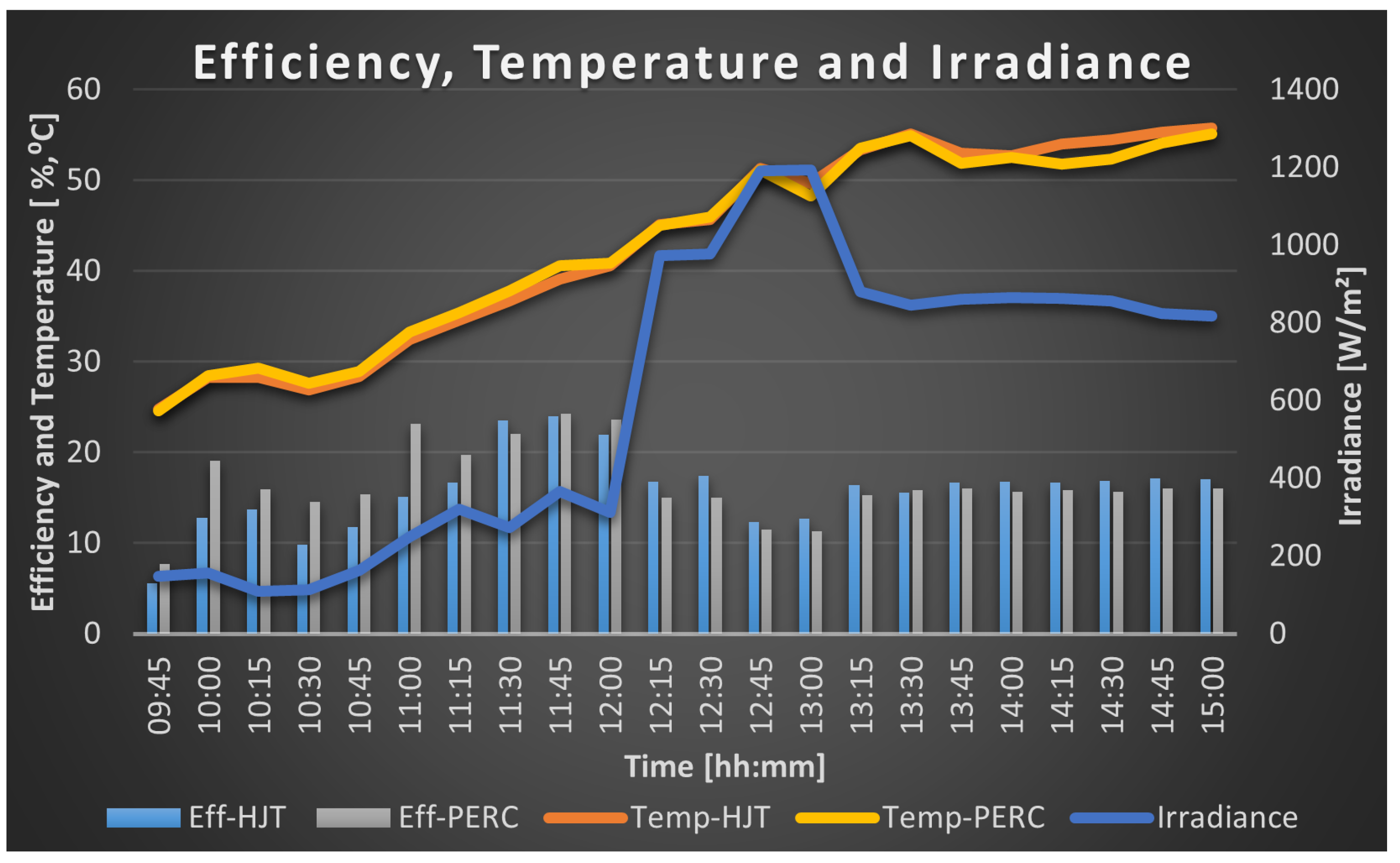
Analysing Table 3 and Figure 18 and Figure 19, it is possible to observe that the HJT panel displayed, on average, 2.21% more efficiency than PERC, during this sunny day.
From 09:15 until 13:15, except for the value read at 12:45, the irradiance slowly rose from 455 to 919.6 W/m2. It was expected that both panel efficiency would follow this trend. However, the maximum efficiency point registered for HJT appeared at 09:45 with a value of 20.68%, a module temperature of 43.7°C, and an irradiance value of 531.6 W/m2. At the same time, PERC obtained a maximum daily value of 16.59% efficiency at 10:45 with a module temperature of 55.7°C and an irradiance value of 719.8 W/m2.
Figure 18.
Module efficiency and temperature for August’s 19th.
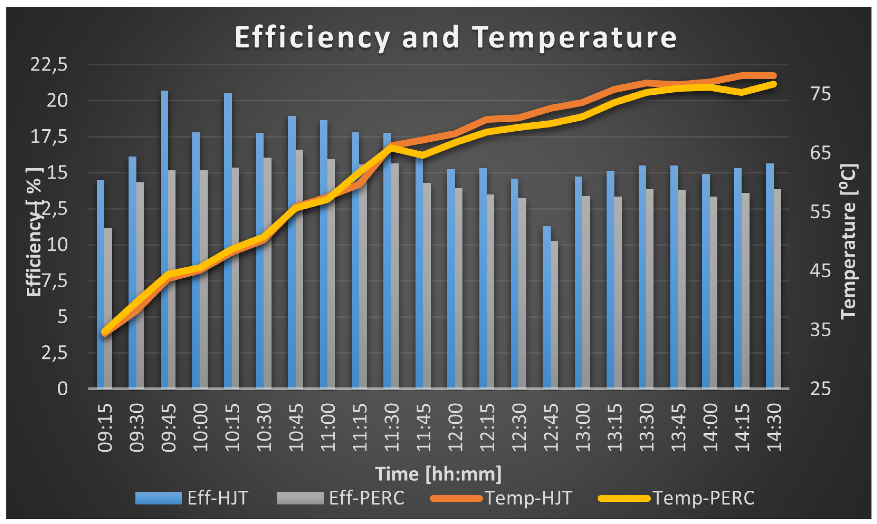
Figure 19.
Irradiance, module efficiency, and module temperature for August’s 19th.
Module temperature continuously raised in both technologies throughout the day. Figure 18 shows that at 11:30, the HJT module and PERC module present 17.75% and 15.64%, respectively. Currently, module temperatures are similar on both technologies, with the HJT presenting 66.2°C and PERC displaying 65.9°C. After this time, both modules’ temperatures kept rising, surpassing 75°C, and efficiency values dropped to around 14/15% on HJT and 13% on PERC.
After noon, except for the measurement taken at 12:45, irradiance values were kept inside the [857.7 W/m2; 919.6 W/m2] range. Although the module temperature has continued to elevate from near 70°C to near 80°C, efficiency values were kept nearly constant.
Note that during the previous day of measurements, on August’s 18th, between 12:15 and 13:00, while the panels were operating under high temperatures (+60°C), an increase in irradiance was reflected in a decrease in efficiency. This situation was again verified at 12:45 on August’s 19th. The HJT panel presented a temperature of 72.6°C, and the PERC module displayed a temperature of 70°C. An increase in irradiance from 908.3 to 1185 W/m2 resulted in a decrease in efficiency of 3.31% in HJT efficiency, while PERC dropped 3.01%.
When irradiance dropped from this day’s highest value to 917.2W/m2, HJT’s efficiency value raised 3.44% while PERC saw his efficiency value climb 3.12%. These results indicate that while performing with high module temperatures, an abrupt increase in irradiance results in a decrease in efficiency, while lowering this significant irradiance value back to the previous values raises efficiency again.
Maximum power was achieved by both modules at 11:30, with the HJT outputting 258.73 W, with a temperature of 66.2°C and an efficiency of 17.75%. The PERC module outputted 248.4 W, with a temperature of 65.9°C and efficiency of 15.64%. The irradiance at this time was 813.1 W/m2.
Performing a similar analysis on the previous day of measurements, the HJT module displays higher efficiency than the PERC panel during the whole day. Despite outperforming PERC with an average of 2,21% efficiency, this value difference is higher while the modules present lower temperatures. As the temperature rises from 66°C, the efficiency difference starts to shorten, and considering the different temperature coefficients, it would have been expected to see a higher efficiency difference benefiting the HJT panel in the presence of higher temperatures.
3.3. 25th of August—Cloudy and Clear Sky Conditions
As can be seen from 09:45 to 12:00 in Table 4 and in Figure 20 and Figure 21, data was collected and low irradiance values were acquired. This reflected the presence of clouds until noon, opening up again and turning into clear sky conditions from 12:15 until 15:30.
Firstly, let’s analyze the data acquired in the presence of clouds. For the first time, it can be seen that, in the ten acquisitions performed between 09:45 and 12:00, the PERC module outperformed the HJT module not only once but eight times. During this time, irradiance values were kept below 370 W/m2, and the modules presented maximum temperatures of 40.6°C for HJT and 40.9°C for PERC. On average, the PERC has outperformed the HJT module by 3.05% in efficiency during this time. This sounds like promising value for the PERC technology to work under cloudy conditions. Between 09:45 and 12:00, the PERC module outputted, on average, 86,71W while the HJT module delivered 69,11W.
Figure 20.
Module efficiency and module temperature for August’s 19th.
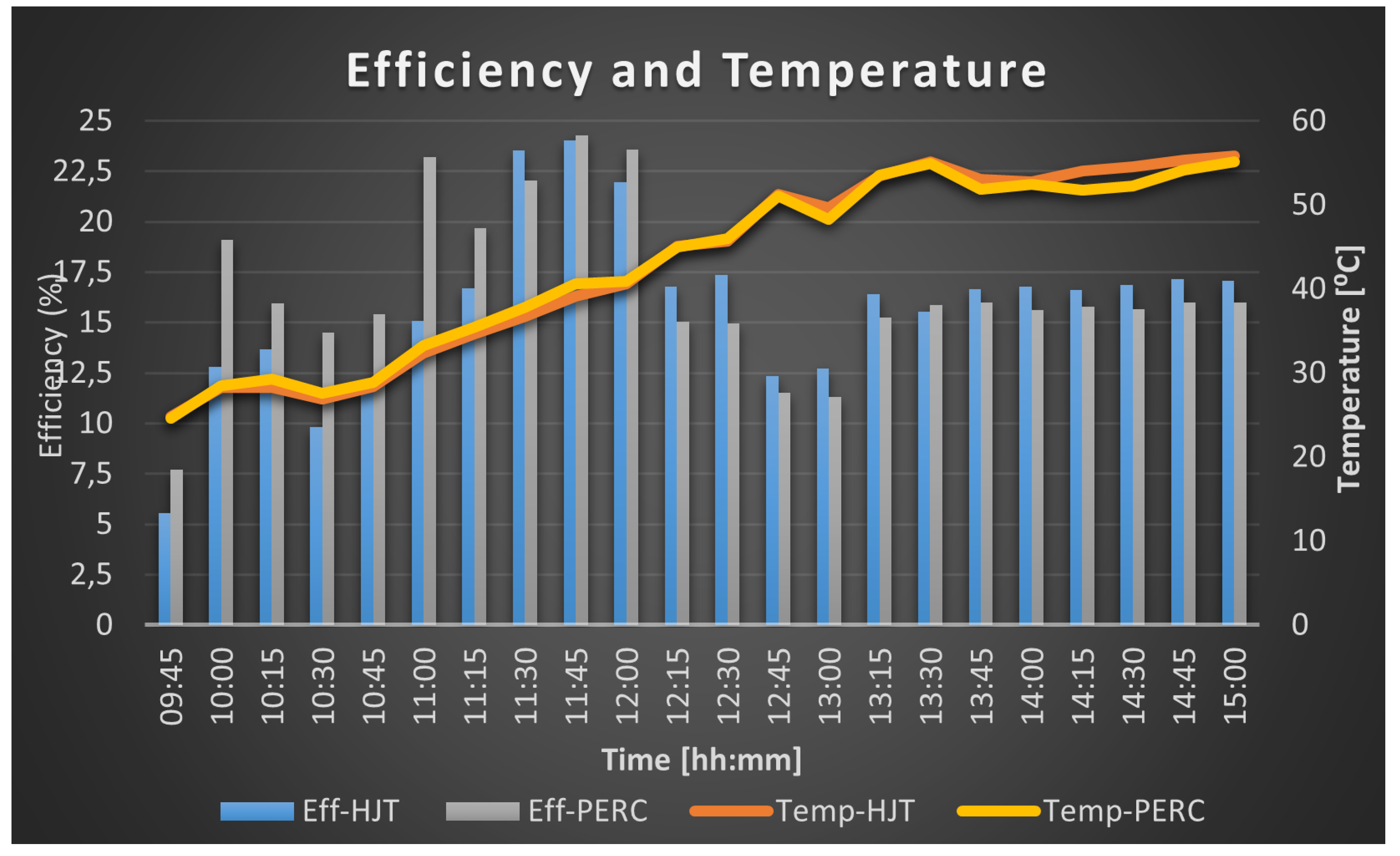
Figure 21.
Irradiance, module efficiency, and module temperature for August’s 19th.
Performing a similar analysis when the sky was free of clouds, from 12:15, it is possible to see that the HJT module outperformed the PERC module until 15:00 regarding module efficiency. On average, the HJT module was 1.11% more efficient than the PERC module. Looking into the irradiance values during this time, it was expected to verify this situation, as this parameter never went below 800 W/m2. Considering the irradiance values, it is possible to divide the analysis into two: one at 12:15 and the other at 13:15. For the first one, it is possible to verify that both modules present better efficiency while the irradiance is below 1000 W/m2. This was verified while module temperature was between 45 and 46°C for both technologies.
The analysis performed for the previous days of data concluded that while modules presented high working temperatures, an increase in irradiance would reduce efficiency. This time, the same situation was verified, but the temperature of the modules did not reach 50°C. It is possible to conclude that a severe increase in irradiance will decrease efficiency independently of the module temperature. This was also verified in the measurements taken at 12:00 and 12:15, where the irradiance values increased from 312.6 W/m2 to 973.3 W/m2, and the efficiency dropped from 21.96% to 16.75% on HJT and from 23.58% to 15.02% on PERC. Despite the drop in efficiency values, the power output in HJT went from 123,08W to 292,4W and from 144W to 285,56W on PERC.
Starting at 13:15, irradiance values decreased and remained under 900 W/m2. This resulted in an increase in efficiency regarding the previous measurement, from 12.7% to 16.4% on HJT and from 11.32% to 15.24% on HJT. Despite the significant increase in efficiency, output power decreased slightly in both modules, reducing approximately 14 W and 2 W on HJT and PERC, respectively.
Maximum power was achieved for the HJT module at 12:30 when the module outputted 304.48 W and displayed an efficiency of 17.37%. The temperature displayed was 45.7°C, and irradiance was 977.6 W/m2. The PERC module achieved maximum power at 12:15 and 12:30, with an output of 285.56 W. Module temperatures were 45°C and 56°C, efficiencies were 15.02% and 14.95%, and irradiance was 973.3 W/m2 and 977.6 W/m2, for the measurements taken at 12:15 and 12:30, respectively.
3.4. 29th of August—Cloudy and Clear Sky Conditions
As can be seen by Table 5, Figure 22 and Figure 23, this day of measurements presented both cloudy, characterized by the low irradiance values from 10:00 to 10:30 and at 11:30, and clear sky situations, characterized by the remaining samples. When performing an analysis when the presence of clouds was confirmed, it is possible to observe that in the four samples taken, the HJT module outperformed the PERC module in terms of efficiency in three of them. Between 10:00 and 10:30, despite being able to display efficiencies in the [31.71%; 33.80%] range for HJT and [29.43%; 36.59%] range for PERC, the power output of the modules did not exceed 83 W. These high-efficiency values were only verified while the irradiance values were kept below 128 W/m2. When irradiance values increase to the [700 W/m2; 900 W/m2] range, power output increases to the [220 W; 301 W] range, and the HJT modules outperform the PERC module, regarding efficiency, in all the measurements taken.
Figure 22.
Module efficiency and module temperature for August’s 29th.
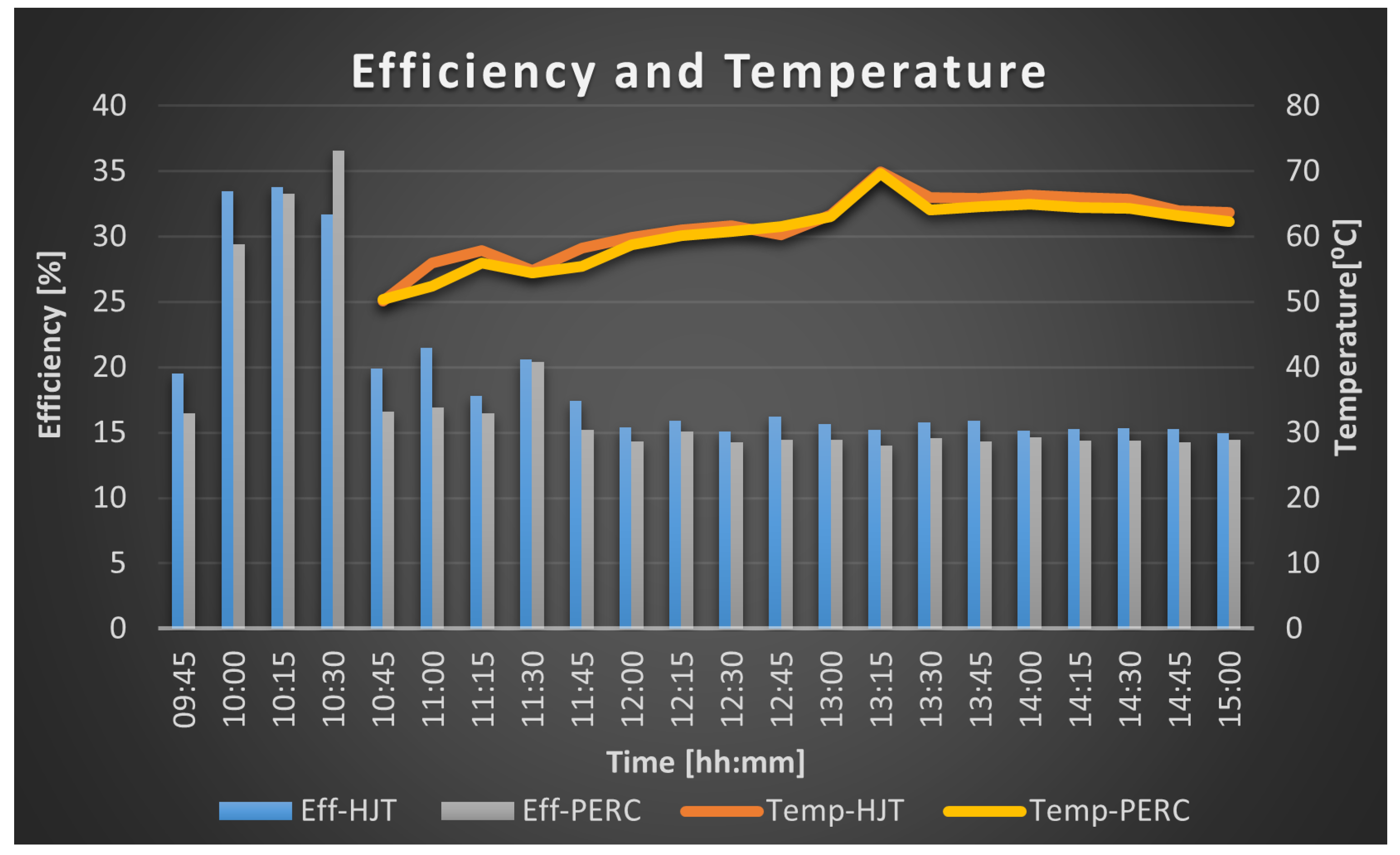
Figure 23.
Irradiance, module efficiency, and module temperature for August’s 29th.
Maximum power was achieved by the HJT module at 11:00, displaying an output of 301.93 W. This daily highest value was obtained with an irradiance of 784.3 W/m2, a temperature of 55.9°C, and the module displayed an efficiency of 21.47%. For the PERC module, the maximum outputted power was achieved at 11:15, with a value of 264.46 W, a module temperature of 56°C, an irradiance value of 821.8 W/m2 and a module efficiency of 16.48%.
It is possible to observe that, from 10:45 until 15:00, except for the measurements taken at 11:30, the irradiance values were kept above 763 W/m2. Regarding efficiency, both modules had their values decreased compared to those obtained in the presence of clouds. The PERC module presented efficiency values in the [13.97%; 16.91%] range, while the HJT module displayed values in the [14.96%; 21.47%]. On average, the HJT module displayed 1.47% more efficiency than the PERC module between 10:45 and 15:00, except for the low irradiance measurement at 11:30.
Compared with the previous measurements, the existence of sudden increases in irradiance was not verified. Instead, at 11:30, a sudden decrease was verified. Irradiance values dropped from 821.8 to 379.9 W/m2. It is possible to observe that efficiencies on both modules increased, from 17.77 to 20.60% on HJT and from 16.48 to 20.38% on PERC. At the next measurement, irradiance increased to values over 800 W/m2 again, and as expected, efficiency values increased.
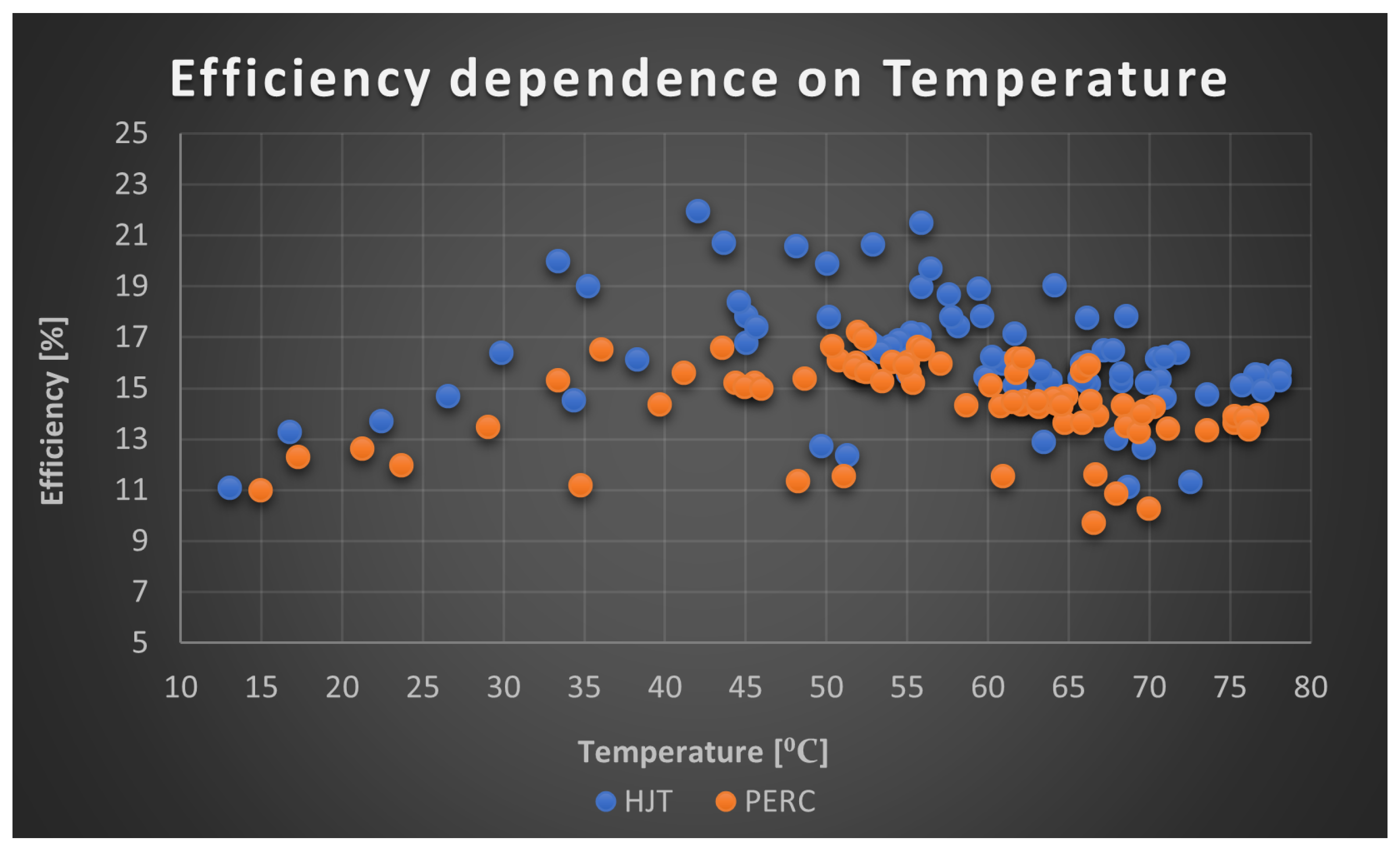
4. Temperature and Irradiance Dependencies on HJT and PERC Efficiencies
After performing several analyses according to each day of meteorological conditions, it is extremely important to compute all the efficiency values on the same graph to obtain a more detailed analysis regarding temperature and irradiance behavior. Only the values under clear sky conditions with irradiance over 250 W/m2 were selected for this section. This can be justified by the extreme performance difference in the presence of clouds, resulting in very high-efficiency values translated to minimal power output due to low irradiance.
It is possible to observe in Figure 24 the behavior of HJT and PERC modules’ efficiency regarding temperature. As expected, it is possible to note the decrease in efficiency of both modules for temperatures above 55°C. This statement aligns with the temperature coefficient definition, in which the modules display less efficiency for increased working temperatures. This data displays the range [35°C; 55°C] of temperature with the best efficiency.
Figure 24.
Efficiency dependence on temperature for HJT and PERC modules.
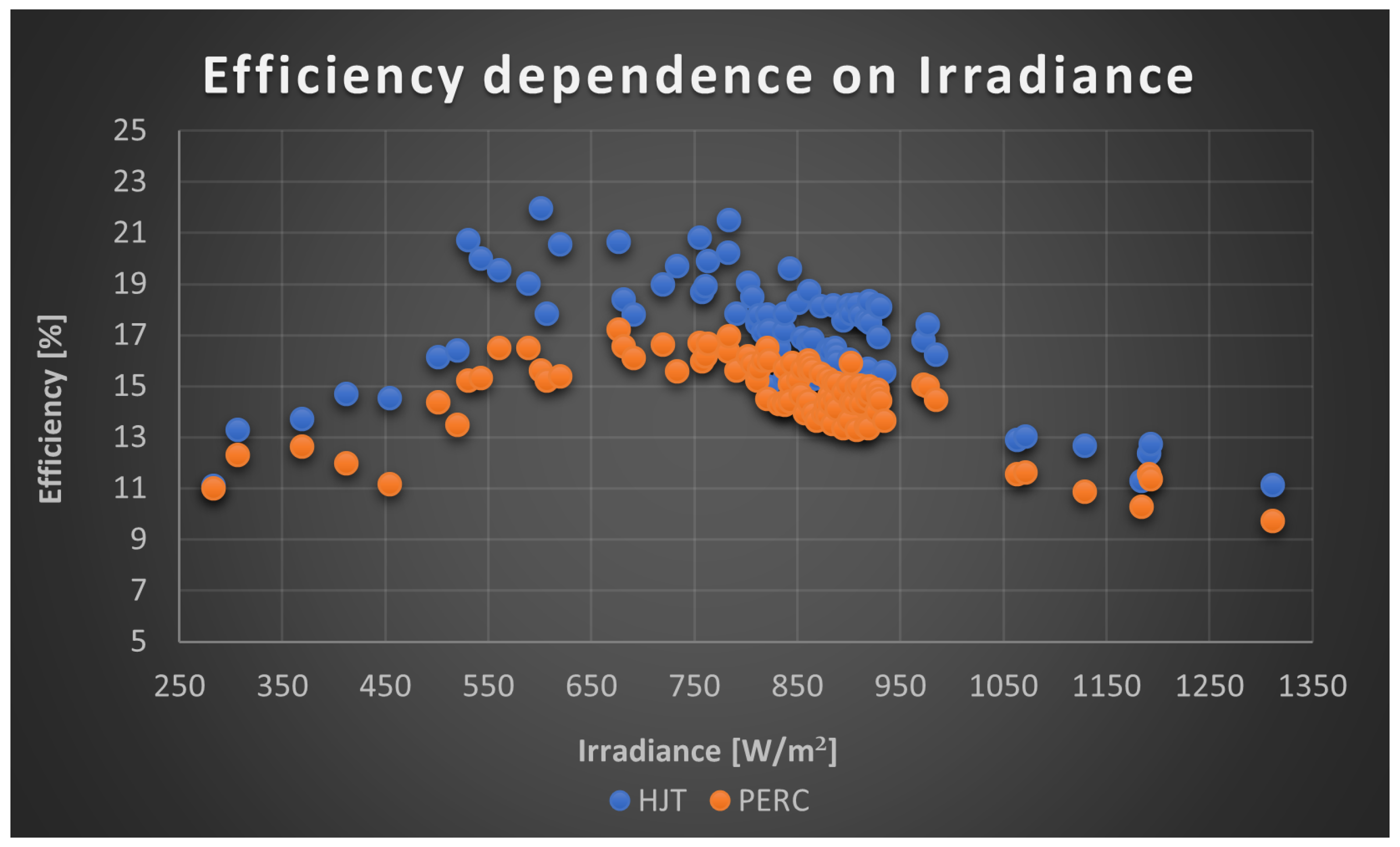
It is shown in Figure 25 the efficiency dependence of irradiance for the HJT and PERC modules. The data gathered in Figure 25 shows an increase in efficiency for both modules until irradiance surpasses 750 W/m2, approximately. For irradiance values above 1000 W/m2, efficiency drops to values close to 10% on both modules. A good irradiance range for modules to work is in [550 W/m2; 975W/m2]. The individual daily analysis stated that the HJT constantly outperformed the PERC module for clear sky conditions, independently of the irradiance shown.
The effect of temperature on module efficiency was analyzed, but no conclusion was drawn that compared the performance of both modules. It was stated in the analysis of Figure 24 that the effect of temperature resulted in an efficiency decrease. This does not compare the different temperature coefficients presented on the datasheets. The PERC module displays a much higher temperature coefficient of -0.350%/°C compared to the -0.259%/°C parameter of the HJT.
Figure 25.
Efficiency dependence on irradiance for HJT and PERC modules.
In Figure 26, the temperature dependence of the modules’ efficiency difference is shown. According to the temperature coefficient values, a bigger difference in efficiency was expected to be seen that would favor the HJT module when entering high temperatures. This was not verified, as the modules present higher differences on temperatures below 50°C.
Figure 26.
Efficiency difference dependence on temperature.
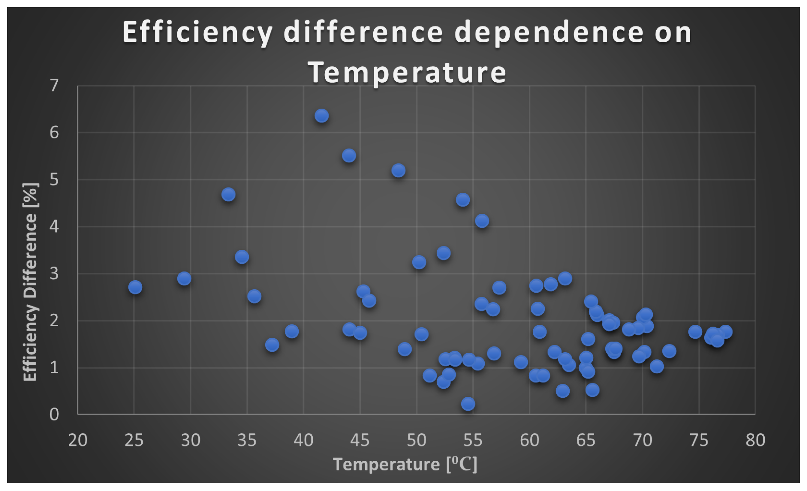
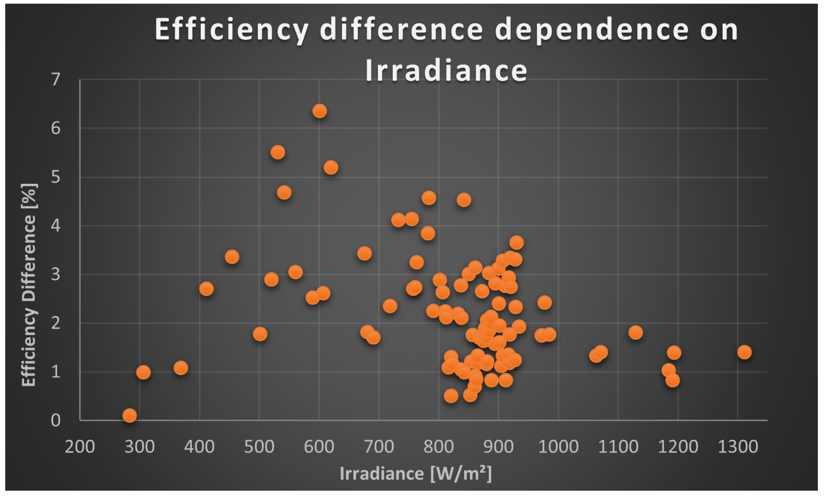
Figure 27.
Efficiency difference dependence on irradiance.
5. Discussion
After analyzing five days of collected data, the most important information is gathered below:
- Under clear sky conditions, regarding efficiency, the HJT constantly outperforms the PERC module;
- Under cloudy conditions, regarding efficiency, the PERC module has displayed higher values than the HJT module in 71,4% of the measurements;
- Despite the PERC module presenting higher power output in STC conditions, experimentally, the HJT module outputs, almost every time, more power than the PERC module;
- A sudden increase in irradiance negatively affects the efficiency, independently of the module temperature. Likewise, a sudden decrease in irradiance will increase module efficiency;
- For the HJT module, maximum power was obtained with an average irradiance of 859.62 W/m2, an average efficiency of 18.78% and an average temperature of 58°C;
- For the PERC module, maximum power was obtained with an average irradiance of 866.26 W/m2, an average efficiency of 15.65%, and an average temperature of 60.03°C;
- Despite the HJT module displaying a better temperature coefficient, the efficiency difference is shortened when the modules present high working temperatures;
- Modules display better efficiency when working under the irradiance range [550 W/m2; 975 W/m2];
- Modules display better efficiency when working under the temperature range [35°C; 55°C].
Case Study and Economical Analysis After analyzing the experimental data, it is possible to compute the average efficiencies of the modules necessary to perform economical analysis and to make conclusions about project feasibility and break-even points.
The modules’ performance under cloudy conditions was not considered for this calculation since they represent much higher efficiency values with low power output. This way, the following averages, according to each measurement day, were computed and displayed in Table 6.
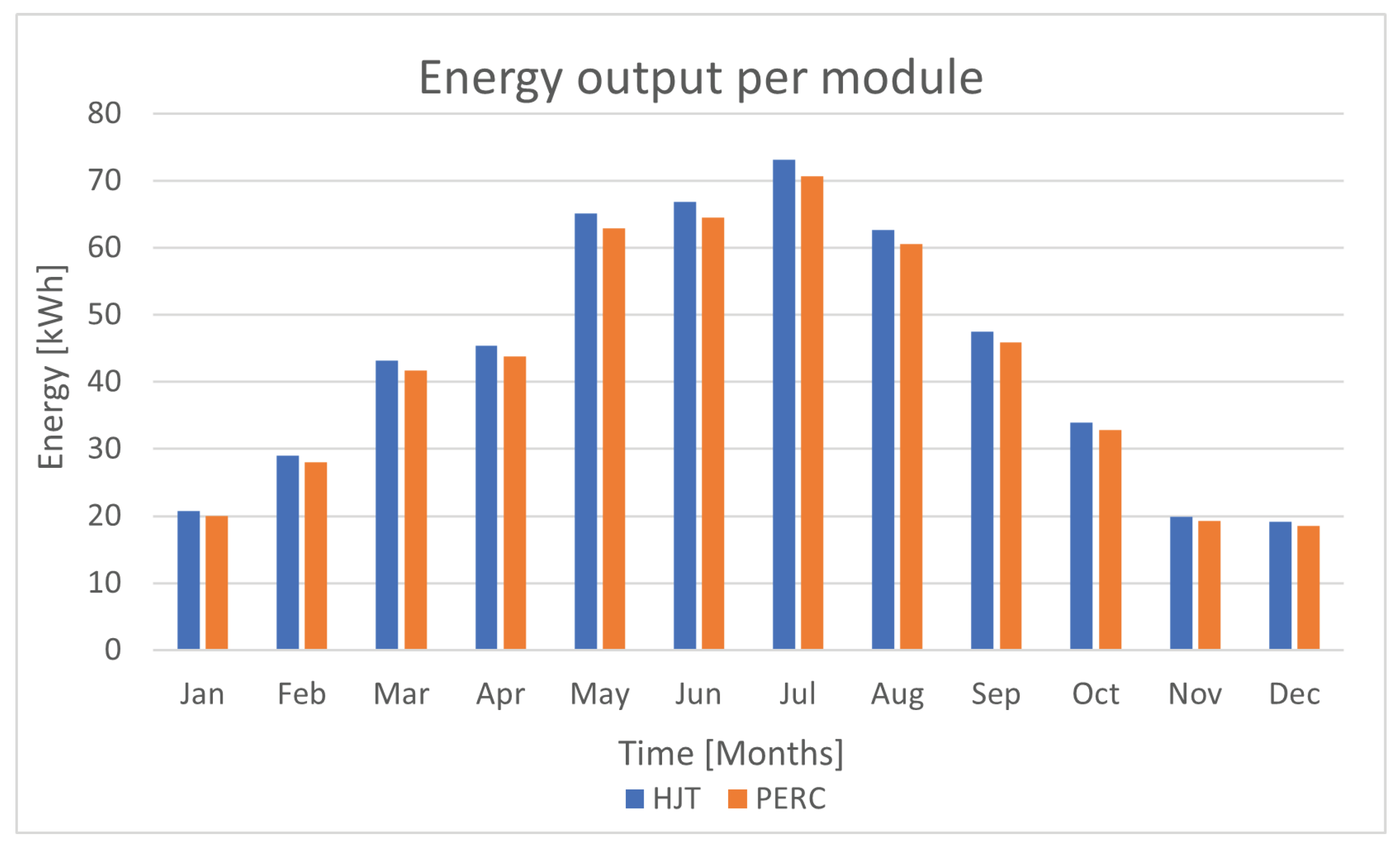
Note that these values represent the efficiency of the system (modules+cable). Using the PVGIS tool [? ], the monthly irradiation, in [kWh/m2], over one year, was computed and is displayed in Figure 28. These values were computed considering the horizontal mounting of the modules on the university location. To compute the module energy output, the equation 2 was used, and values obtained are displayed in Table 7 and in Figure 29.
Figure 28.
Monthly irradiation during the year 2020.
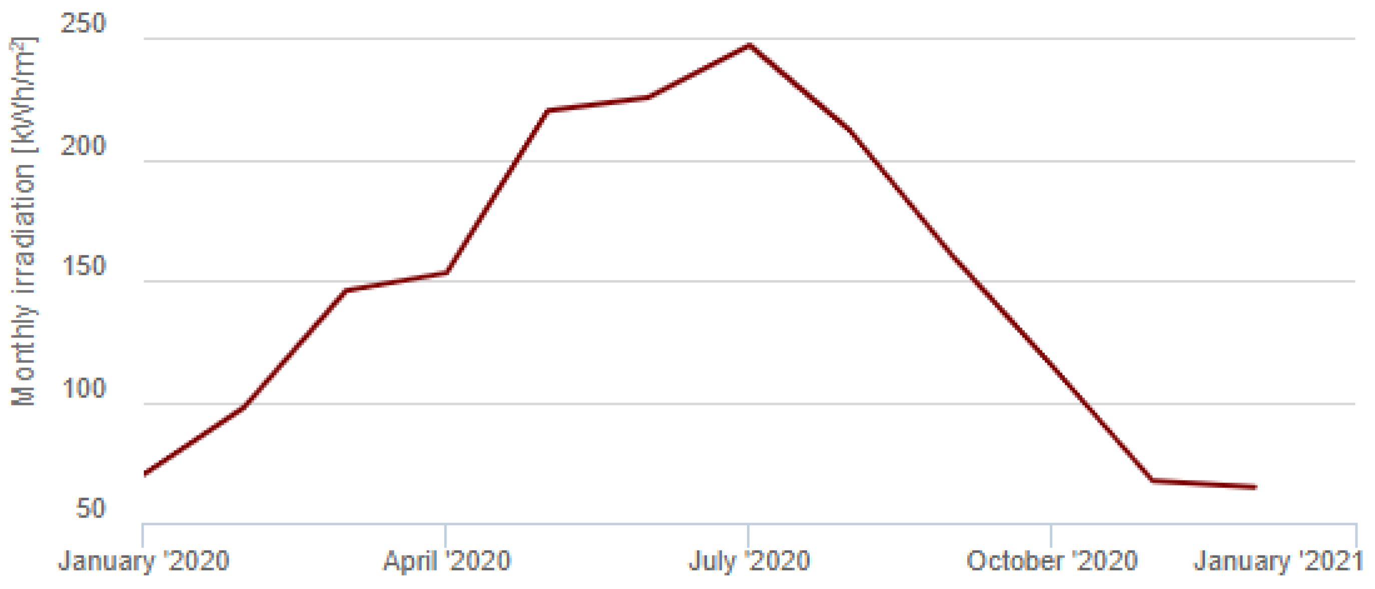
Figure 29.
Energy output per month of 1 module of HJT and 1 module PERC technology.
Searching for different electricity suppliers in Portugal for 2022 and their respective tariffs, Table 8 was computed. As several values are displayed, and there is a substantial difference between the least and the most expensive tariff, the average value of 0.18424 €/kWh was considered to perform a fair analysis.
The values in Table 7 consider the system used in the laboratory experiments. However, five projects will be computed to analyze the economic feasibility of using these different modules. The first three projects will cover fixed power installations. These simulate a situation where the system’s constraint is total power installed. Since both modules present similar nominal power per square meter, 206.40 W/m2 on HJT and 202.28 W/m2 on PERC, the power constraint is equivalent to having an area constraint. Results from these cases will conclude which technology is best suited to implement on installations like house rooftops, factories’ rooftops, and photovoltaic parks.
Two other projects with fixed investment costs will be simulated. The installation constraint is now the system’s cost. Results from these cases will conclude which technology is better suited to implement in situations where the system area is now not considered.
6. Projects with a Fixed Power Installation
6.1. 4.5 kW Project
An installation of 4.5 kW was considered. This case compares 12 PERC modules, with 4740 W in STC, and 13 HJT modules, referenced with 4810 W in STC. This way, the for each of (module + cables) is the same value verified in Table 6, 16.51% for HJT and 14.63% for PERC.
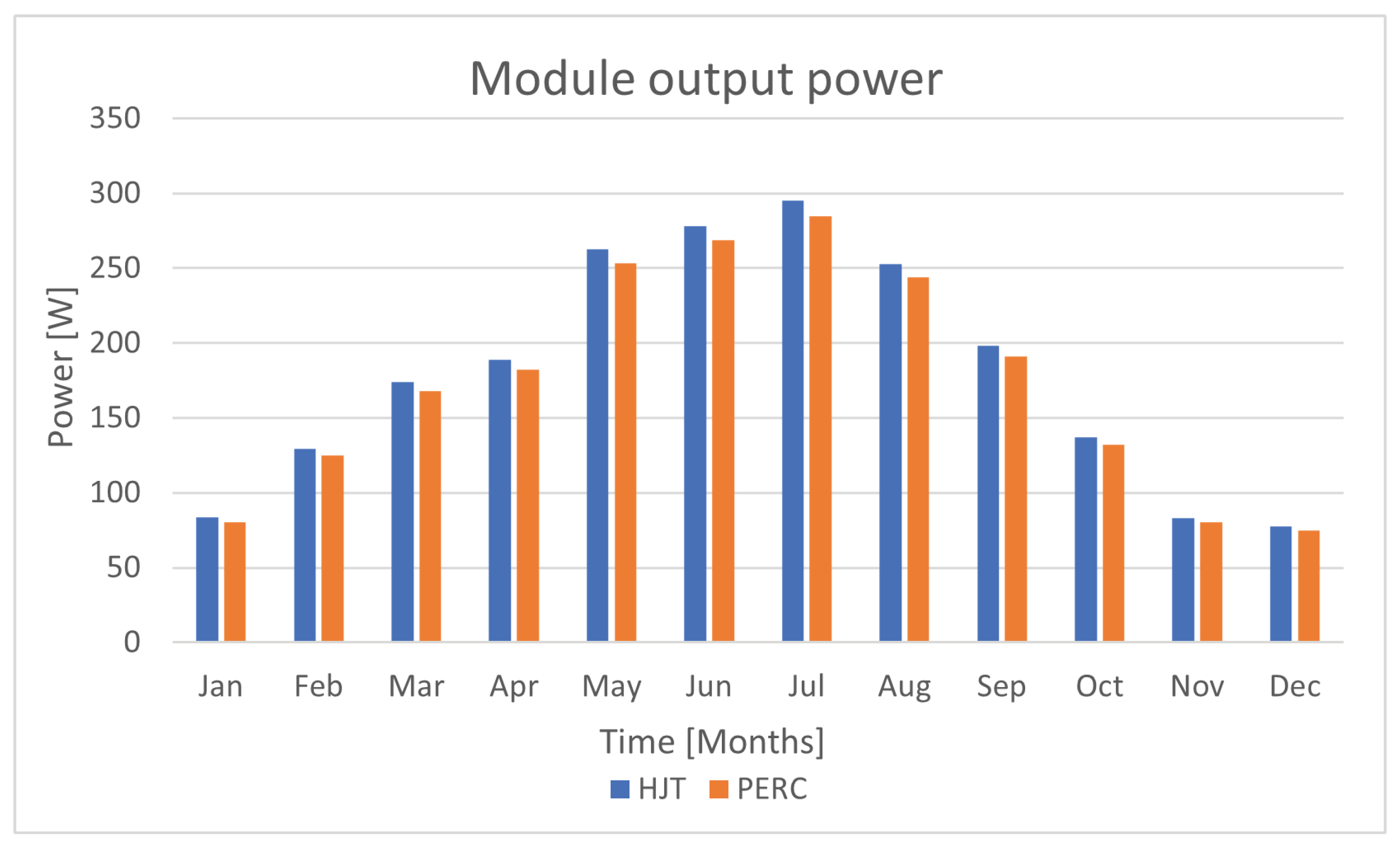
It is mandatory to compute the average power output to choose an inverter that displays higher efficiency with the system power output. Considering that a day has, on average, 8 hours of sun throughout the year and the data presented in Table 7, module power was achieved by dividing the monthly energy output by the total hours of daylight during a month, presented in Table 9 and in Figure 30.
The month with the highest average power production is July, with an average of 295 W delivered on HJT and 284.76 W outputted on PERC. Knowing that the system is composed of 13 HJT modules and 12 PERC modules, the system will output, on average, in July, 3835 W for the HJT system and 3417,12 W for the PERC system. Based on these values and consulting the market, choosing the best inverters for each system is possible. For the HJT system, the PRIMO 4.0-1 with 4000 W nominal power was chosen. The PRIMO 3.5-1 inverter with 3500 W nominal power was then chosen for the PERC system.
Figure 30.
Average power delivered by each module for each month.
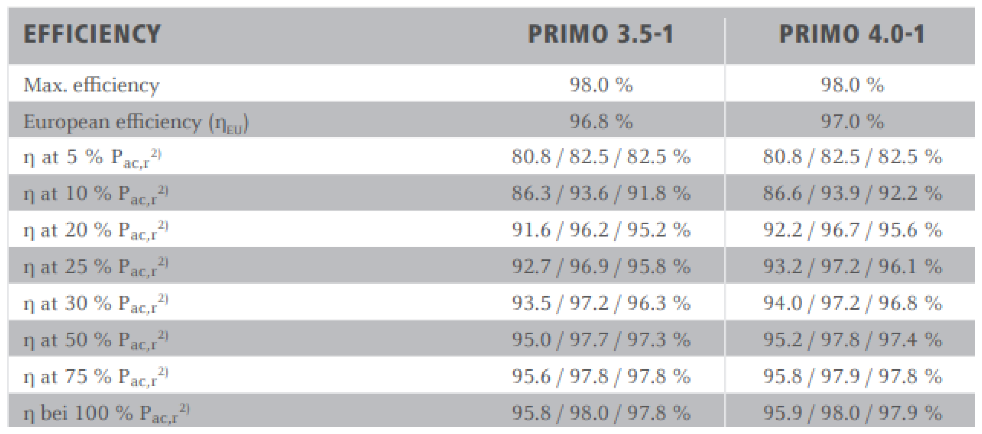
Inverter efficiencies strongly depend on the available power input. This results in a variation of the inverter efficiency during the year that must be considered when calculating this project. As stated in Table 9, 295 W was the average power produced in July for HJT, while 284.76 W corresponded to the PERC module. The Table 10 will display the annual system average output divided by the nominal power of the inverter.
Figure 31 displays the inverter efficiency regarding the input power. It is possible to observe in Figure 31 that there are three displayed efficiencies for each nominal power value. This is verified due to the different behaviors that the inverter displays when different voltage levels are available on the input. As this project case is based on power input/output, an average of these three voltages was performed and is displayed in Table 11. With Table 10, it is possible to display the inverter efficiency for each month of the year, as shown in Table 12.
Figure 31.
Inverter efficiencies regarding power input.
It is now possible to compute the final energy output of each system and compare it. Applying the inverter efficiencies present in Table 12 to the module’s energy output present in Table 7 and multiplying by the number of modules in each system, it is possible to obtain the final energy outputted by each system monthly and annually, as can be seen in Table 13 and in Figure 32.
Figure 32.
Energy produced by HJT and PERC system for a year.
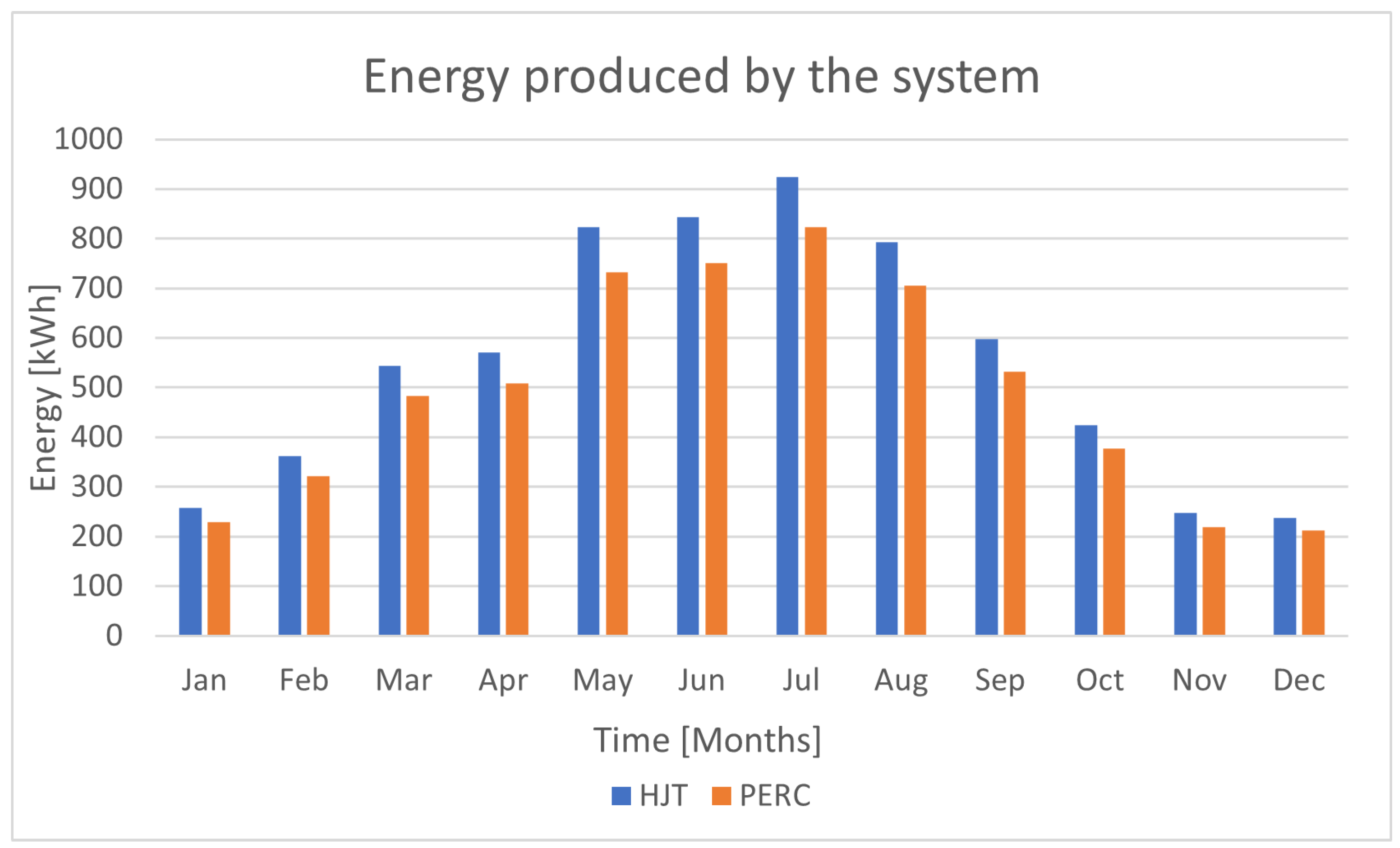
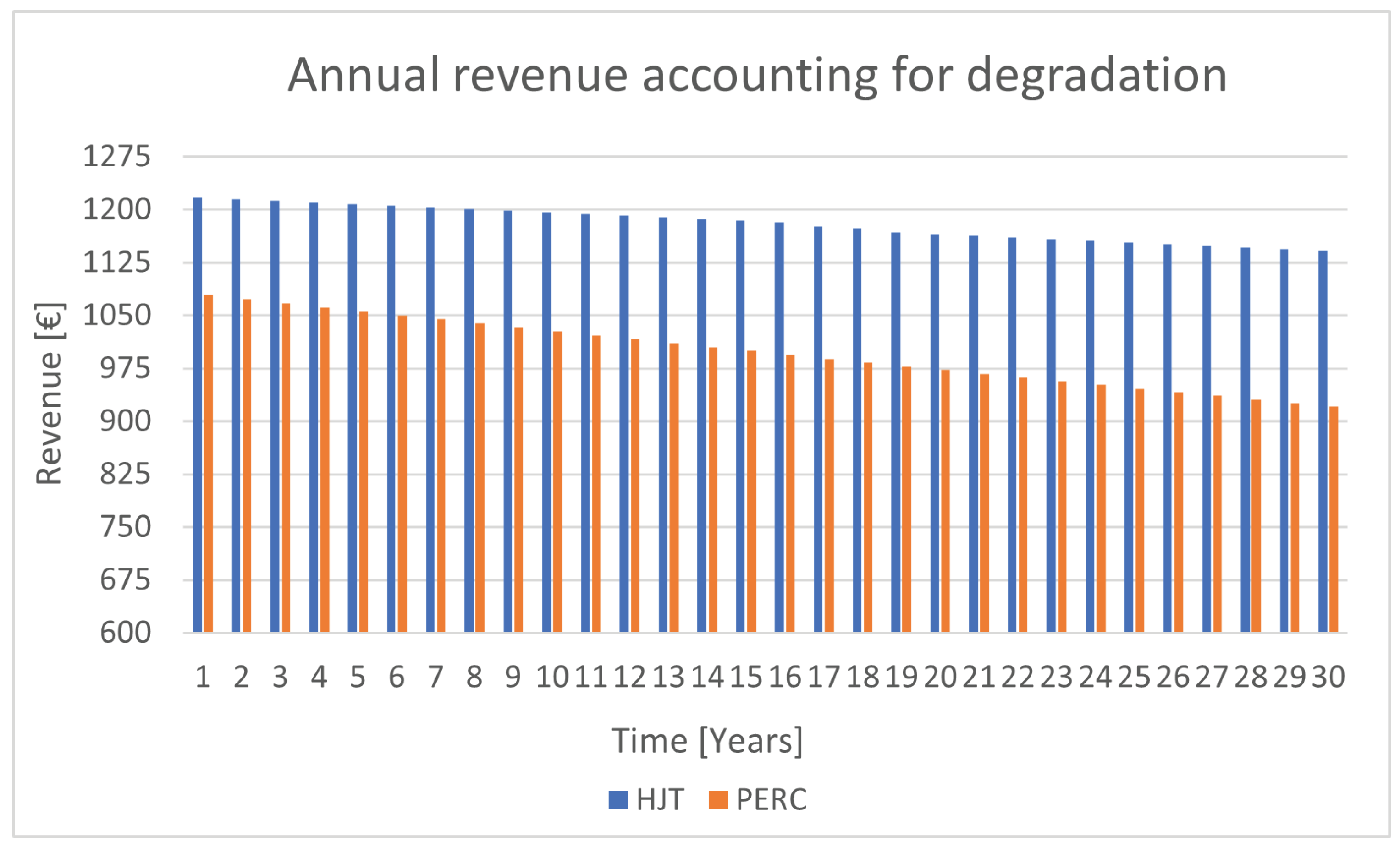
With an annual production of 6622.28 kWh for the HJT system and 5890.55 kWh for the PERC system and considering an average price of 0.18424 €/kWh, it is possible to save annually 1220.09 € and 1085.27 €, respectively, with the HJT and PERC system. There is a maximum degradation of 0.20 % of nominal power per year for the HJT module, and the manufacturer displays both power and product warranty for 30 years. For the PERC module, the manufacturer displays a degradation of 0,55% of nominal power per year while offering a 12-year product and 25-year linear power output warranty. It is then possible to compute the monetary value of the converted energy accounting for degradation during 30 years, as seen in Table 14 and in Figure 33. It is also possible to compute the cumulative production for 12, 15, 20, and 30 years as displayed in Table 15.
Figure 33.
Annual revenue of HJT and PERC system accounting for module degradation for 30 years.
After computing the production of the systems using HJT and PERC technology, it is now required to compute the respective costs. The HJT module was sold for 271.385 € per unit when this research was performed. Hence, 3528€ was the value to pay for 13 modules. Regarding PERC technology, modules had a unitary price of 154.16€. Twelve modules would cost 1849.92€.
Regarding inverters, the PRIMO 4.0-1 had a cost of 1389.00€ [? ] for the HJT system, while the PRIMO 3.5-1 had a cost of 1314.99€ [? ] for the PERC system.
Regarding cables, 100 meters were sold for 140 € [? ]. With an approximation of 200 m of cables being used by each system, 280 € was added to the cost of each system. A horizontal structure that supports more than 10 modules was considered to assemble both systems on horizontal rooftops and cost 781.82 € [? ]. Finally, 1000 € was considered labor to assemble the whole system.
Considering all previous costs, the final system prices can be displayed in Table 16.
With the costs and the production of the systems computed, it is possible to see in Figure 34 the cumulative profits of these systems for 30 years. In Table 17, it is possible to observe the profits for years 12, 15, 20, and 30 as well as the Average Profit per Year (APpY) and the Average Return on investment (AROI) by year. APpY value can be computed by dividing the cumulative profit for a selected year by the number of years since the investment has begun, displayed in equation 3. AROI can be calculated as displayed in equation 4. Note that this equation is similar to the Return on Investment (ROI) equation 5, but instead of considering the annual profit, it considers the cumulative profit until the designated year.
Figure 34.
Cumulative profits of HJT and PERC systems throughout 30 years-4,5 kW installation.
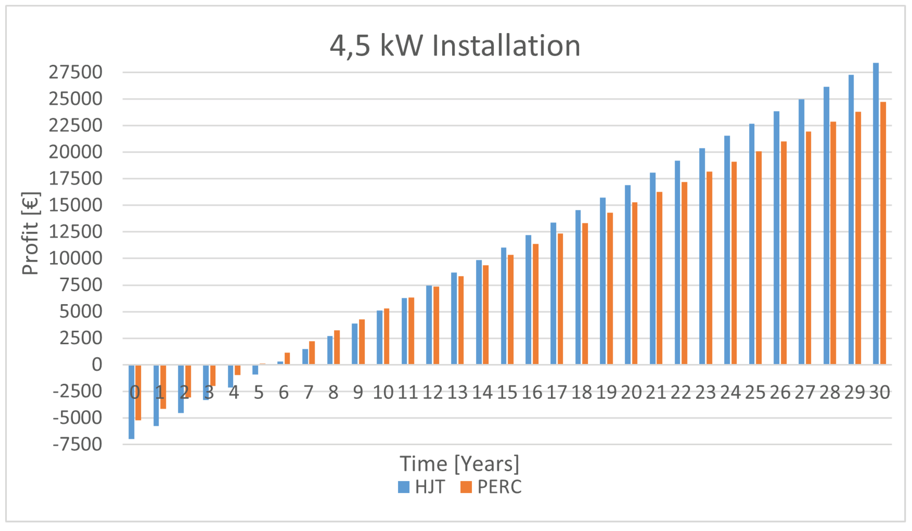
The results obtained indicate that the PERC system would achieve the break-even point, where costs and revenues cancel each other, during the 5th year, while the HJT system would achieve the break-even point during the 6th year. After this time, they will turn into a lucrative investment. It is possible to see in Figure 34 that, despite displaying more costs and therefore lowering the annual return on investment, the HJT system can be considered a better investment and will deliver more profit over the long run. During the 12th year, the HJT system surpasses the revenue of the PERC system and displays better Average Profit per Year over long periods.
6.2. 3.5 kW Project
To simulate a 3.5kW project, ten modules were considered for the HJT system and nine for the PERC system. The remaining costs, such as cables, horizontal structure, inverters, and labor, were assumed to be the same as in the previous case. System costs can be visualized in Table 18. With the costs and the production of the systems computed, it is possible to see in Figure 35 the cumulative profits of these systems for 30 years. In Table 19, it is possible to observe the profits for years 12, 15, 20, and 30 as well as the APpY and AROI.
Figure 35.
Cumulative profits of HJT and PERC systems throughout 30 years-3,5 kW installation.
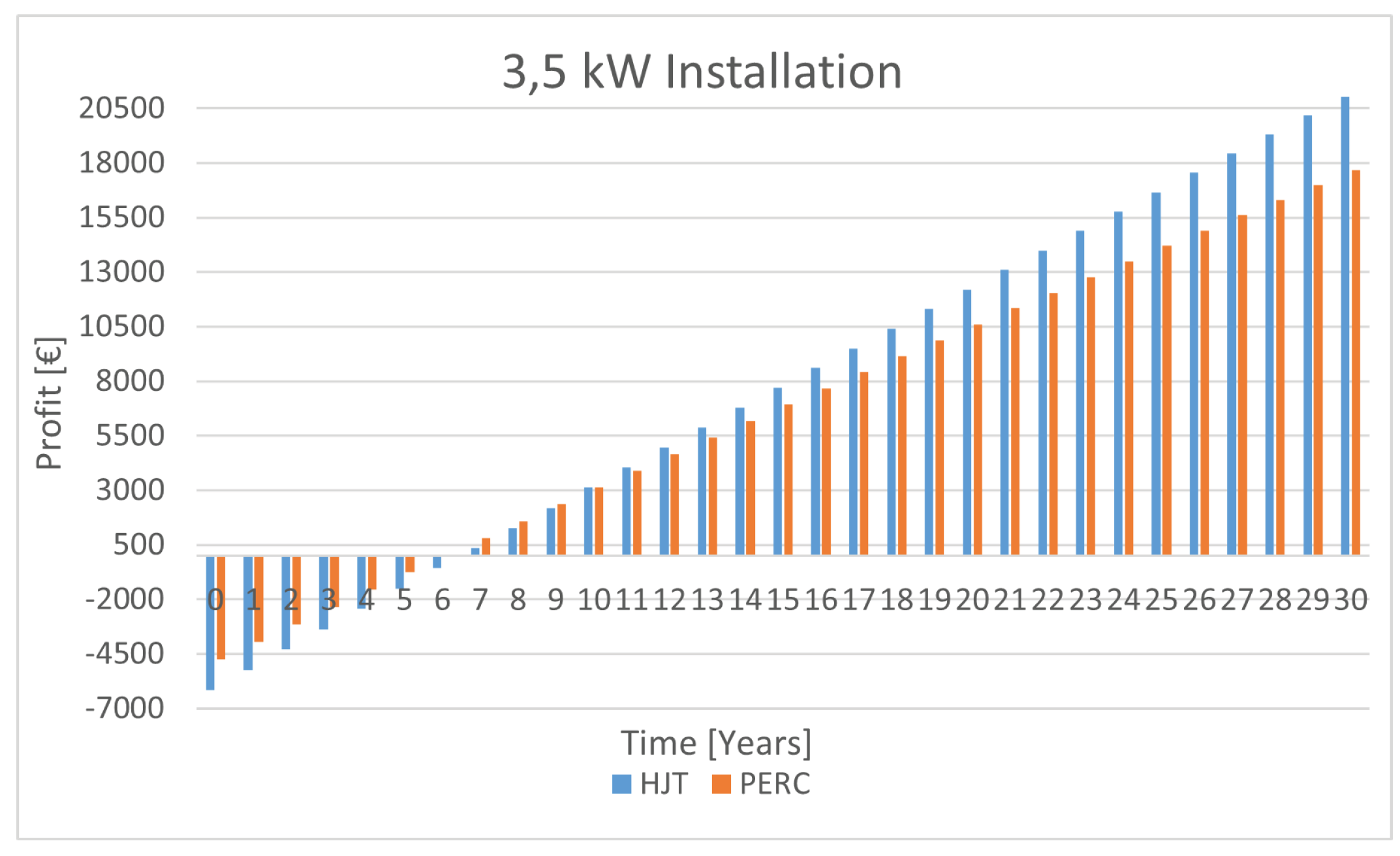
For a 3.5 kw case, the PERC system would achieve the break-even point during the 6th year, while the HJT system would achieve the break-even point during the 7th year. After this time, they will turn into a lucrative investment. Similar to the 4.5 kW installation, in the long run, the HJT system will deliver more profits than the PERC system despite the bigger investment costs and having a lower Annual Return on investment. During the 11th year, the HJT system surpasses the revenue of the PERC system.
6.3. 2.5 kW Project
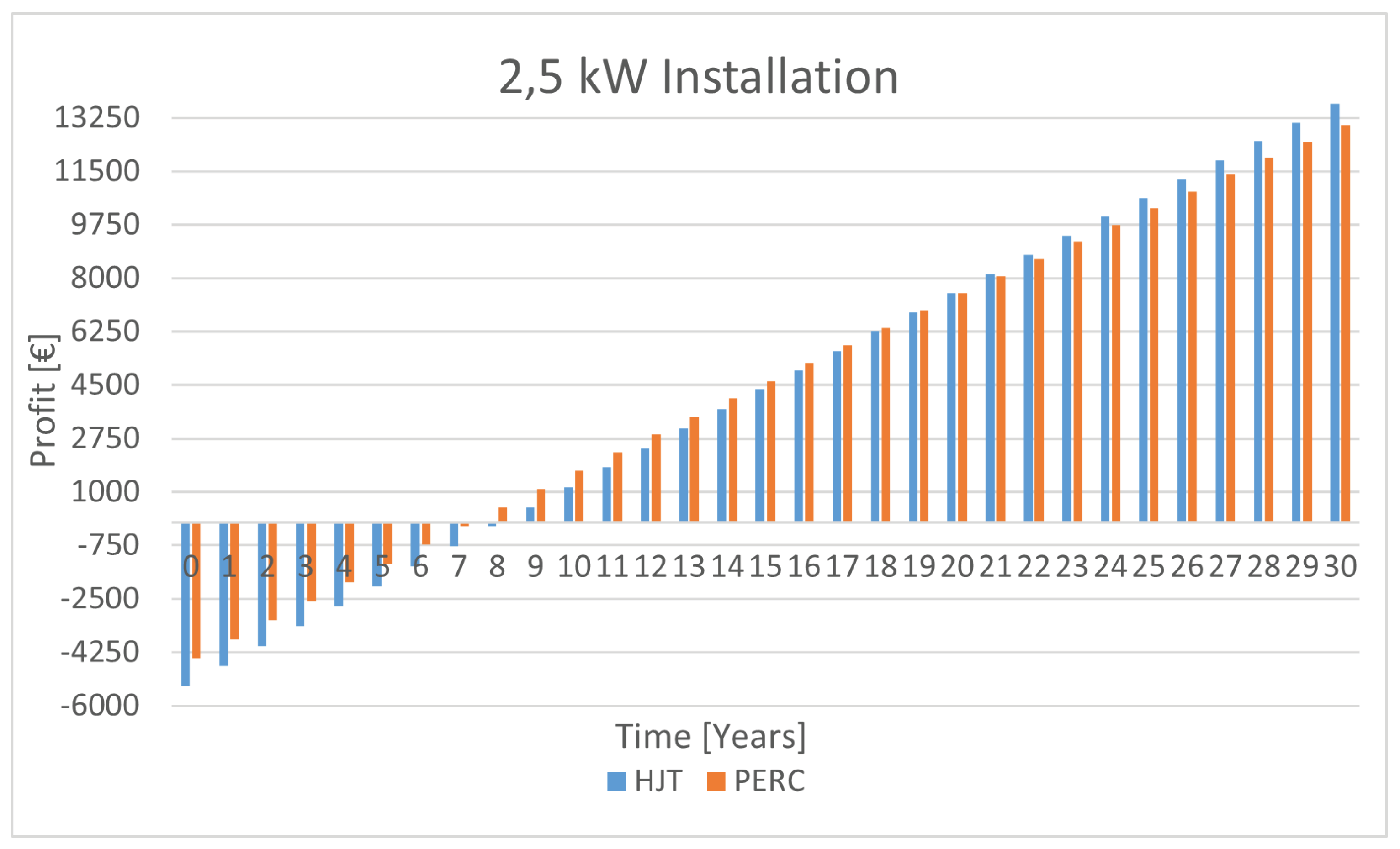
To simulate a 2.5kW project, 7 modules were used for the HJT and PERC systems. The remaining costs, such as cables, horizontal structure, inverters, and labor, were assumed to be the same. System costs can be visualized in Table 20. With the costs and the production of the systems computed, it is possible to see in Figure 36 the cumulative profits of these systems for 30 years. In Table 21, it is possible to observe the profits for years 12, 15, 20, and 30 as well as the APpY and AROI.
For this 2.5 kW case, the PERC system would achieve the break-even point during the 8th, while the HJT system would achieve the break-even point during the 9th year. After this time, they will turn into a lucrative investment. Similar to the 3.5 kW installation, in the long run, the HJT system will deliver more profits than the PERC system again despite the bigger investment costs and lower Annual Return on investment. During the 20th year, the HJT system surpasses the revenue of the PERC system.
Figure 36.
Cumulative profits of HJT and PERC systems for 30 years - 2,5 kW installation.
6.4. Fixed Power Installations—Conclusions
After simulating 4.5 kW, 3.5 kW, and 2.5 kW nominal power installations, it is possible to conclude that:
- When comparing fixed power installations, it is possible to compute that a PERC system displays a better Annual Return on investment than an HJT system. This explains the reduced time that the PERC installation requires to achieve the break-even point;
- Despite displaying lower AROI, the HJT system will deliver more profit over time and will surpass the PERC system in the long run regarding profit.
- As the installed power decreases, the amount of time that the HJT installation requires to surpass the PERC installation profits increases. This happens due to the fixed installation costs. As less power is required, the number of photovoltaic modules decreases, and the costs related to the cables, inverter, labor, and structures are more significant in comparison with the total investment costs;
- Likewise, when the installed power increases, the HJT installation will require less time to surpass the PERC installation profits;
- When there is an installation with power constraints or installation area, choosing a system composed of HJT modules will be more profitable.
6.5. 5000 € Investment Project
After performing three fixed power installations, two projects with fixed investment values were studied. The first one is considered an installation of 5000€. The same costs as the 4.5 kW project for cables, inverters, structures, and labor were considered, as listed in Table 22. With the costs and the production of the systems computed, it is possible to see in Figure 37 the cumulative profits of these systems for 30 years. In Table 23, it is possible to observe the profits for years 12, 15, 20, and 30 as well as the APpY and AROI.
Figure 37.
Cumulative profits of HJT and PERC systems for 30 years- 5000€ installation.
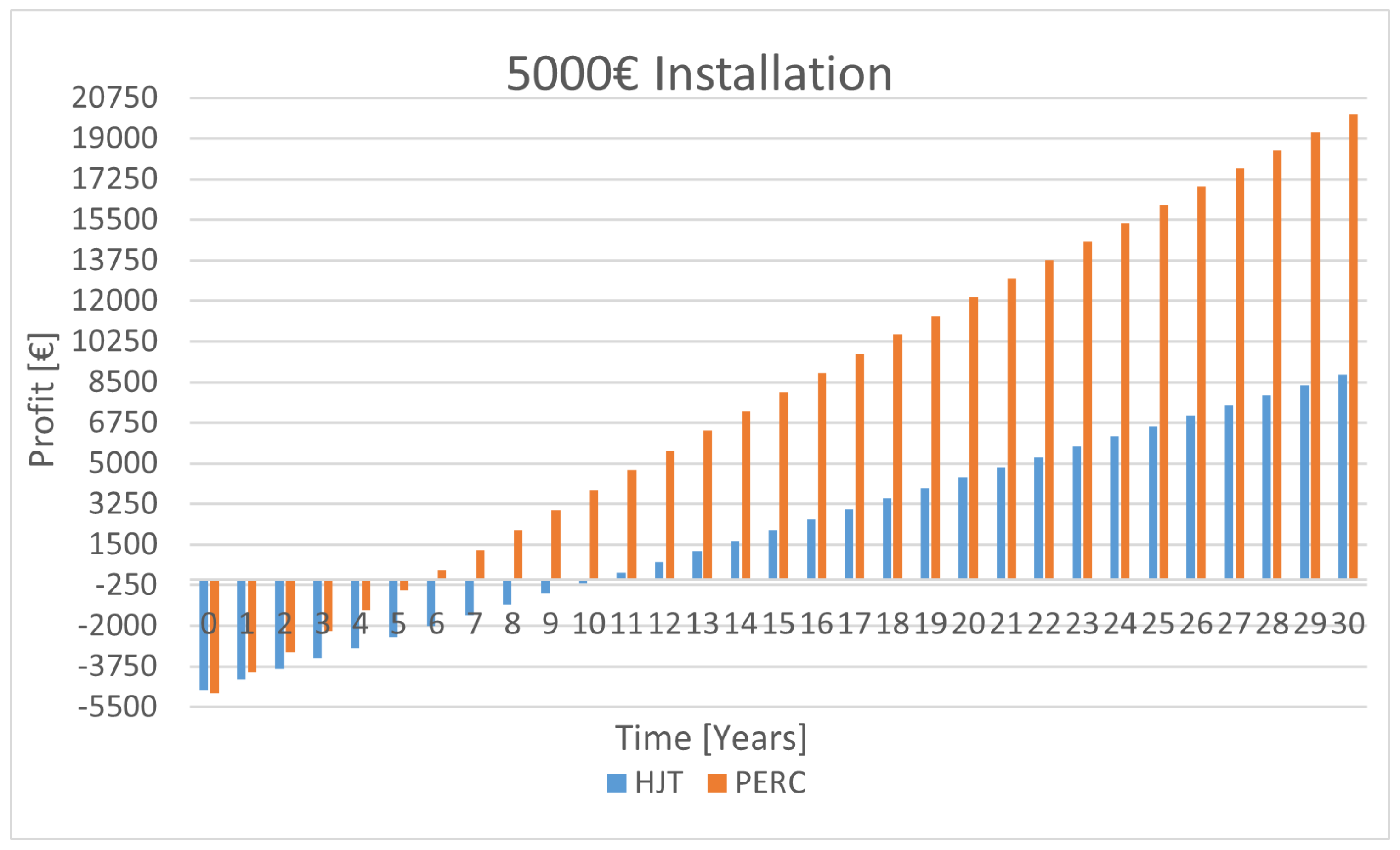
The results indicate that the PERC system would achieve the break-even point during the 6th, while the HJT system would achieve the break-even point during the 11th year. After this time, they will turn into a lucrative investment. Unlike the fixed power installations, the PERC system displays much higher profits than the HJT installation and is never surpassed in profit. Throughout 30 years, the PERC system has displayed a much higher AROI than the HJT system.
6.6. 10000 € Investment Project
One considers now an installation cost of 10000€. Since the number of modules increased to 17 on HJT and 25 on PERC, new inverters are required for the HJT system [? ] and for the PERC system [? ]. The amount of cable increased by 50% on HJT and doubled on the PERC system. Regarding structures, both systems doubled these from the previous example. Labor costs also increased in the same proportion as cables. These new costs are listed in Table 24.
With the costs and the production of the systems computed, it is possible to verify in Figure 38 the cumulative profits of these systems over 30 years. In Table 25, it is possible to observe the profits for years 12, 15, 20, and 30 as well as the APpY and AROI.
Figure 38.
Cumulative profits of HJT and PERC systems for 30 years- 10000€ installation.
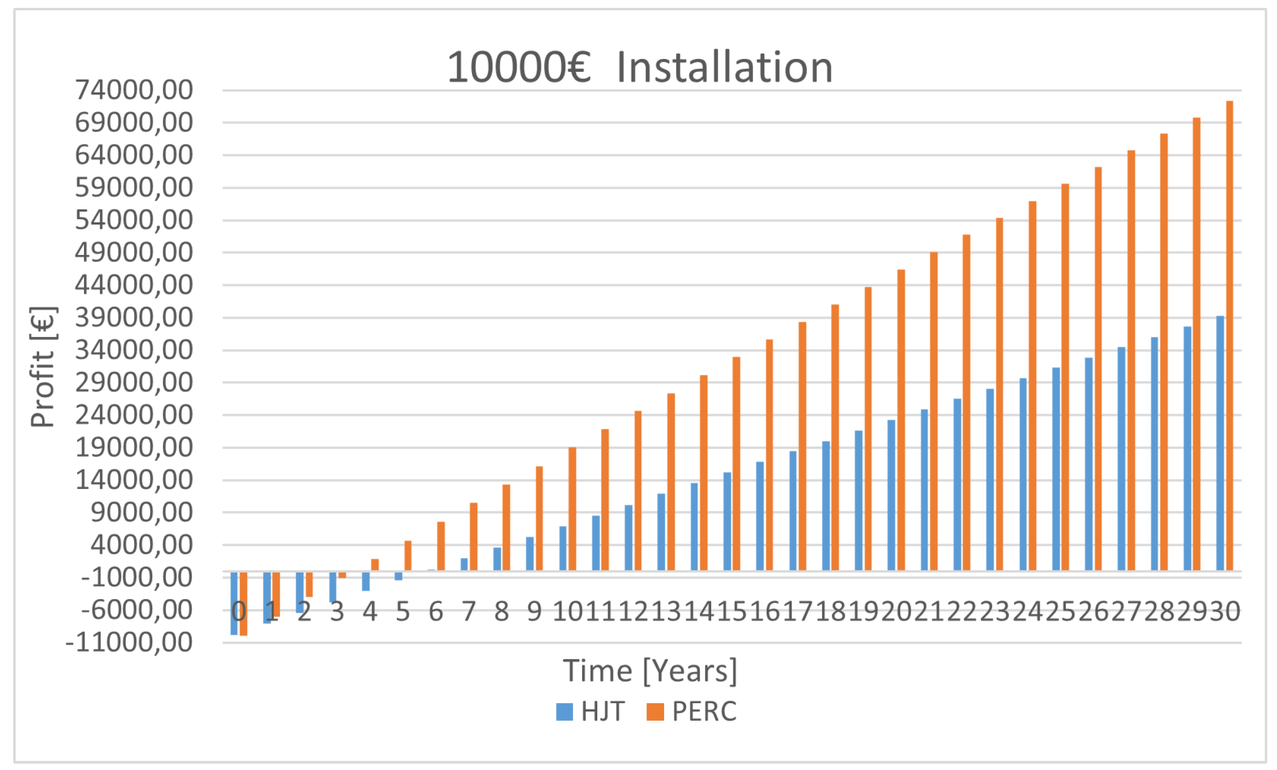
For a 10000 € investment project, the results point to the PERC system achieving the break-even point during the 4th, while the HJT system would achieve the break-even point during the 6th year. After this time, they will turn into a lucrative investment. Similar to the 5000 € installations, a big difference in profit and AROI benefits the PERC installation.
6.7. Fixed Investment Installations - Conclusions
After analyzing the cases of 5000 € and 10000 € installations, it is possible to conclude:
- The PERC system will return more profit in comparison with the HJT installation;
- The PERC system displays much higher AROI than the HJT system;
- When the budget of the installations increased from 5000 € to 10000 €, both installations suffered components updates. Despite this, since the PERC modules are cheaper, an increased budget reflects a bigger increase in the number of modules compared to the HJT system. This way, the remaining system components suffered a bigger intervention on the PERC system. This explains the smaller visual difference in the profits on the 10000 € system, visualized in Figure 38, in comparison to the 5000 € system, visualized in Figure 37.
- When there is an installation with investment constraints, choosing a system composed of PERC modules is a better investment.
6.8. HJT and PERC Modules Malfunction and Replacement
Five projects have already been studied for 30 years. It is important to note that the PERC modules only display 12 years of product warranty. If modules stop working from year 13, will not replace these devices. Since the HJT modules display 30 years of product warranty, it is also important to compute a situation where PERC modules fail outside of the warranty. As HJT modules displayed better economic performance with fixed power installations and the warranty discussion will only influence the PERC modules if there is failure under 30 years, it will be interesting to compare the fixed investment installations to understand if the PERC modules, if replaced, are still a better investment option than the HJT modules.
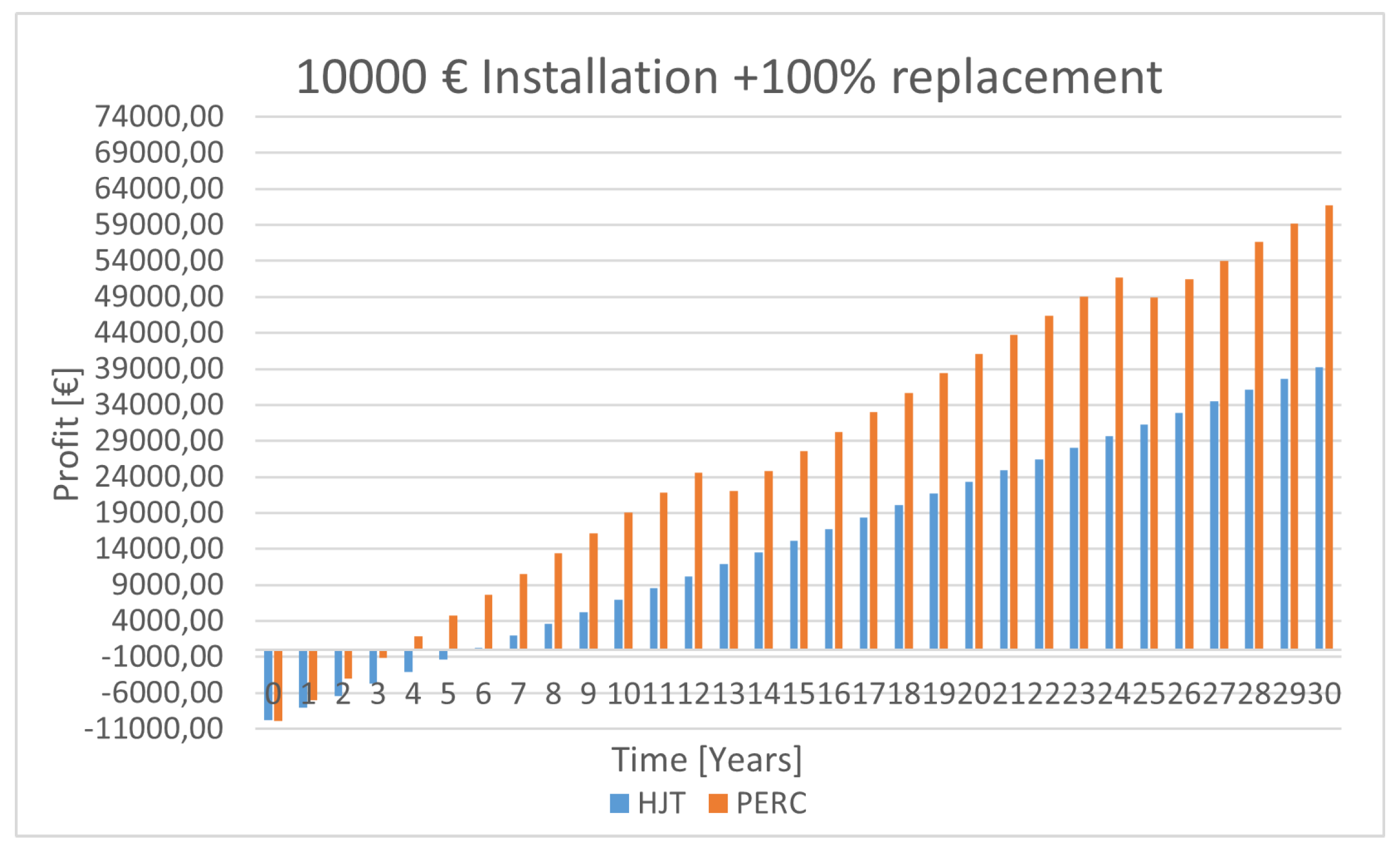
The 10000 € installations will be analyzed in this section. Various simulations were performed, from replacing 10% of the modules to replacing 100% of them. Since there was no displayed major difference until there was a need to replace 100% of the modules, the worst-case scenario will be displayed. The whole number of modules, 25, will need replacement every 12 years. 1500 € of labor was considered for the two necessary replacements in years 13 and 25. Twenty-five modules account for a total of 3854€.
Figure 39 displays the new cumulative profits. It is possible to conclude that even in the worst-case scenario, for a 10000€ installation, PERC is the technology that should be chosen to perform fixed investment installations.
Figure 39.
Cumulative profits of HJT and PERC systems for 30 years- 10000€ installation with module replacements at years 13 and 25.
Figure 39.
Cumulative profits of HJT and PERC systems for 30 years- 10000€ installation with module replacements at years 13 and 25.
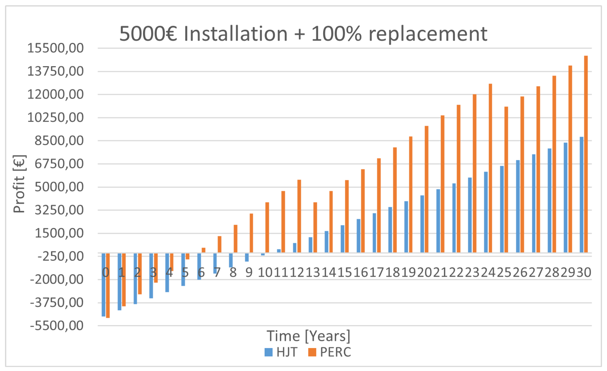
Now, the same situation applies to the 5000 € installations. Ten modules will be replaced in years 13 and 25, costing 1541€ in modules and 1000€ in labor for each intervention. The new cumulative Profits are displayed in Figure 40. It is possible to conclude that even in the worst-case scenario, for a 5000€ installation, PERC is the technology that should be chosen to perform fixed investment installations.
Figure 40.
Cumulative profits of HJT and PERC systems for 30 years- 5000€ installation with module replacements at years 13 and 25.
Figure 40.
Cumulative profits of HJT and PERC systems for 30 years- 5000€ installation with module replacements at years 13 and 25.
7. Conclusions
The HJT module had outperformed the PERC module in conditions where irradiance surpassed the 300 W/m2 value by an average of 1,88%. In the presence of clouds, the PERC module displayed better efficiency, but analyzing that both modules output low power due to the lack of irradiance, this difference could be neglected.
After collecting data that characterizes module behavior, it was possible to simulate the performance of some installations and compare the economic performance. It was concluded that, in the presence of installations with constraints of installed power or installation area, it is better to choose the HJT technology for these projects. As the nominal power will be similar, the more expensive and more efficient HJT modules will turn more profitable in the long run, despite both installations achieving the break-even point considerably fast, making them good investments.
When projects have limited investment, PERC is the technology that should be used in the installations. The lower costs of the modules allow for more modules to be installed, which will compensate for the slightly lower efficiency displayed in the experimental analysis. For this type of installation, even considering the worst-case scenario where the PERC modules need to be replaced as soon as the warranty expires, it was concluded that they were still the viable solution to search for.
Although experimental analysis has been performed and conclusions about the performance of two technologies were taken, there is still some future work that can be carried out:
- Installation of the modules oriented directly to the sun to optimize exposure and increase output power, and the HJT module can receive irradiance from both sides, increasing its efficiency;
- Installation of two modules of each technology in which one of the modules does not receive any cleaning to understand and compare the performance of these effects on the output;
- Compare HJT technology with other technologies that have been raising interest over the last years, such as Interdigitated Back Contact (IBC) cells and tunnel oxide passivated contact (TOPcon) cells;
- Introduce cooling techniques to understand the effect of temperature in a module with the same irradiance and study the economic feasibility of these new projects;
References
- PVPS, I. PHOTOVOLTAIC POWER SYSTEMS PROGRAMME ANNUAL REPORT 2020. Technical report, IEA PVPS, 2020.
- Hezel, R.; Jaeger, K. Low-temperature surface passivation of silicon for solar cells. Journal of the Electrochemical Society 1989, 136, 518. [Google Scholar] [CrossRef]
- Lotsch, H.K.V. High Efficient Low Cost Photvoltaics: Recent Developments; Springer, 2020.
- Jaeger, K.; Hezel, R. A novel thin silicon solar cell with Al2O3 as surface passivation. IEEE photovoltaic specialists conference. 18, 1985, pp. 1752–1753.
- Schmidt, J.; Werner, F.; Veith, B.; Zielke, D.; Steingrube, S.; Altermatt, P.P.; Gatz, S.; Dullweber, T.; Brendel, R. Advances in the surface passivation of silicon solar cells. Energy Procedia 2012, 15, 30–39. [Google Scholar] [CrossRef]
- Kray, D.; Hermle, M.; Glunz, S.W. Theory and experiments on the back side reflectance of silicon wafer solar cells. Progress in Photovoltaics: Research and Applications 2008, 16, 1–15. [Google Scholar] [CrossRef]
- Lotsch, H.K.V. High Efficient Low Cost Photvoltaics: Recent Developments; Springer, 2020; p. 110.
- Mikolášek, M. Silicon Heterojunction Solar Cells: The Key Role of Heterointerfaces and their Impact on the Performance. In Nanostructured Solar Cells; Das, N., Ed.; IntechOpen: Rijeka, 2017; chapter 4. [Google Scholar] [CrossRef]
- Hoex, B.; Heil, S.; Langereis, E.; Van de Sanden, M.; Kessels, W. Ultralow surface recombination of c-Si substrates passivated by plasma-assisted atomic layer deposited Al 2 O 3. Applied physics letters 2006, 89, 042112. [Google Scholar] [CrossRef]
- Söderström, T.; Papet, P.; Ufheil, J. Smart wire connection technology. the 28th European Photovoltaic Solar Energy Conference, 2013, pp. 495–499.
Figure 1.
Rear surface passivation scheme [3].
Figure 1.
Rear surface passivation scheme [3].
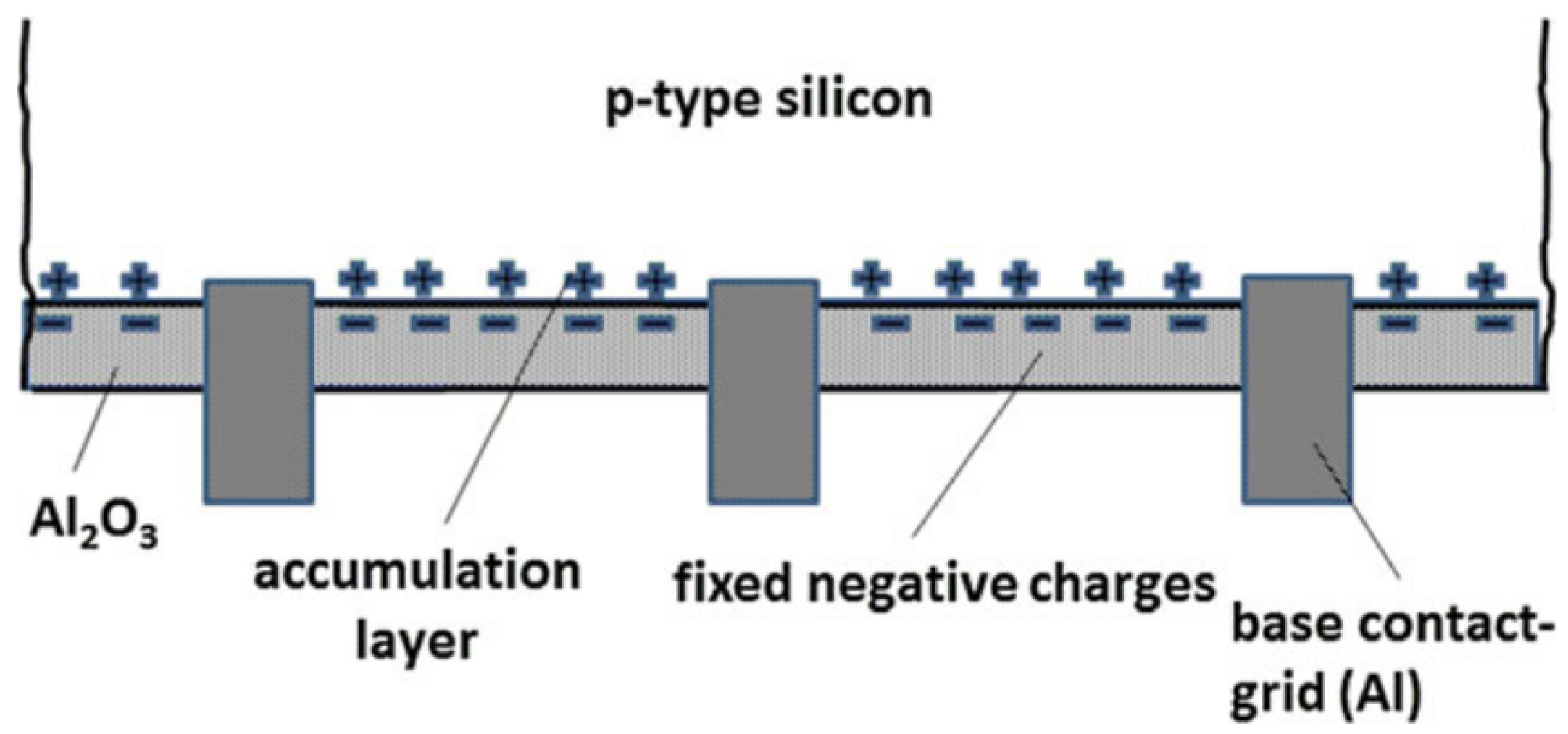
Figure 2.
PERC cell scheme.
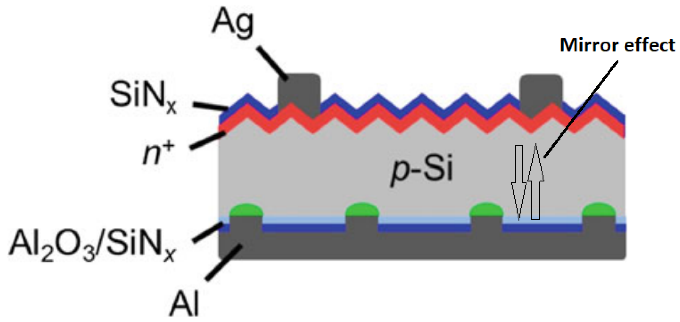
Figure 3.
Efficiency decrease related with LID.
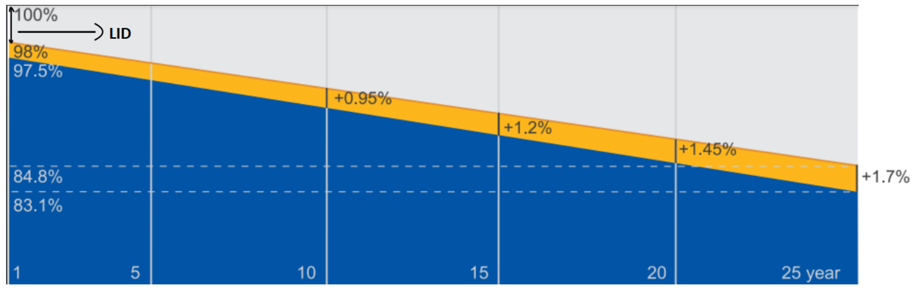
Figure 4.
Cross sectional view of SHJn and SHJp [8].
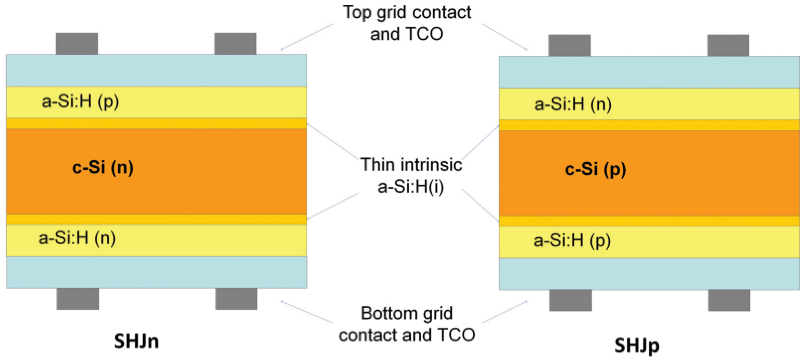
Figure 5.
Busbar vs SWCT [10].
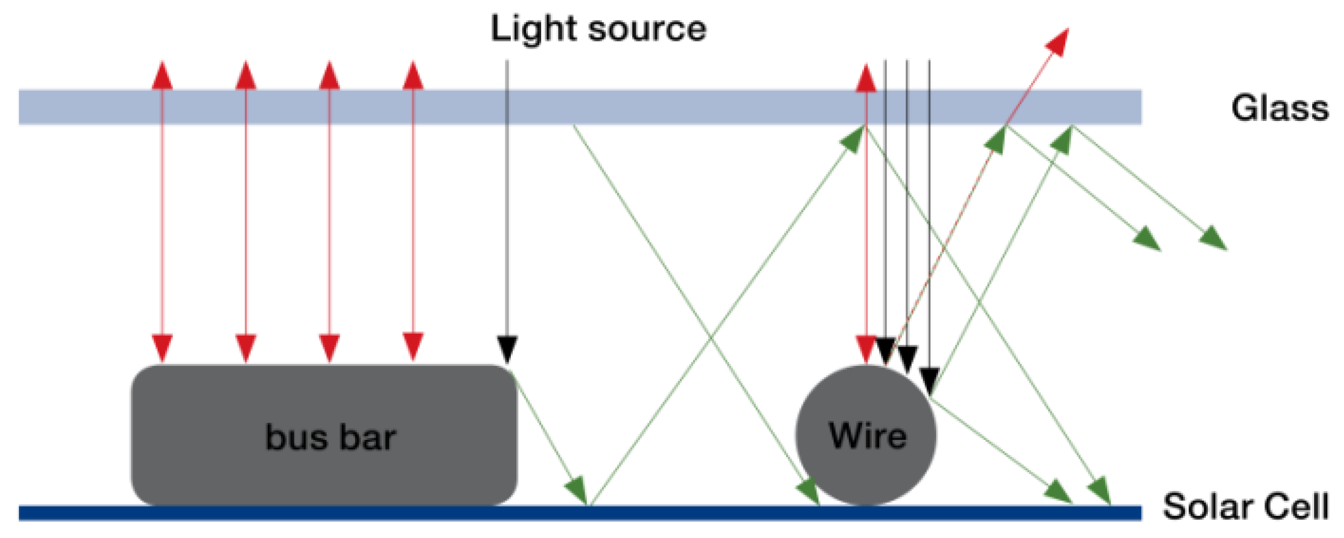
Figure 6.
PERC panel datasheet parameters.
Figure 7.
HJT datasheet parameters - 1.
Figure 8.
HJT datasheet parameters - 2.
Figure 9.
Modules displaced horizontally.
Figure 10.
Rooftop connection - 1.
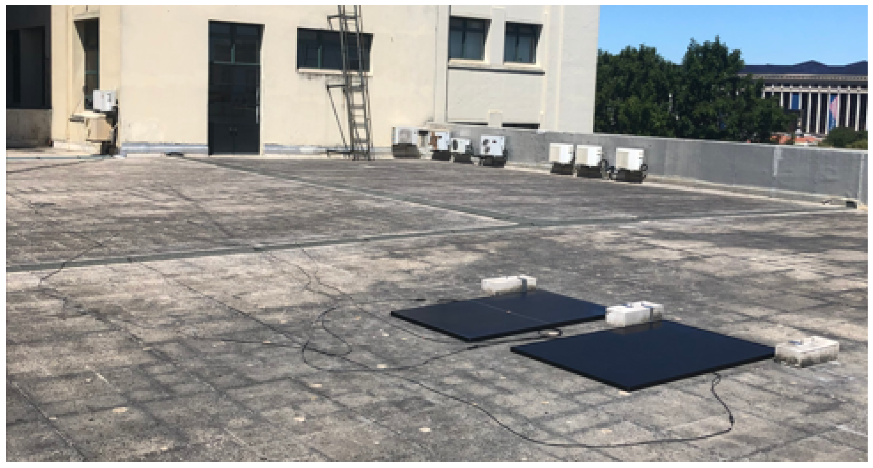
Figure 11.
Laboratory connection - 1.
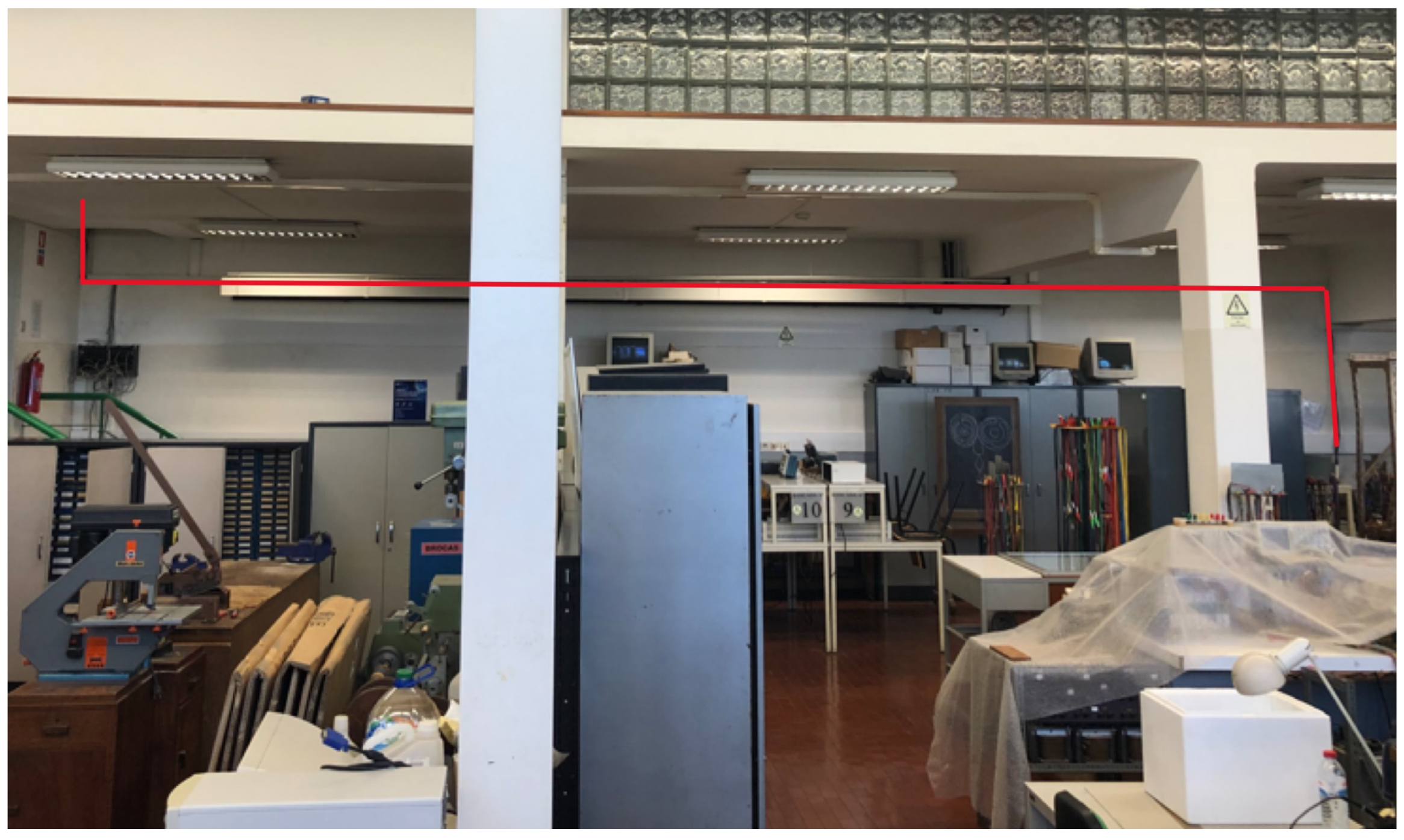
Figure 12.
Final acquisition system used.
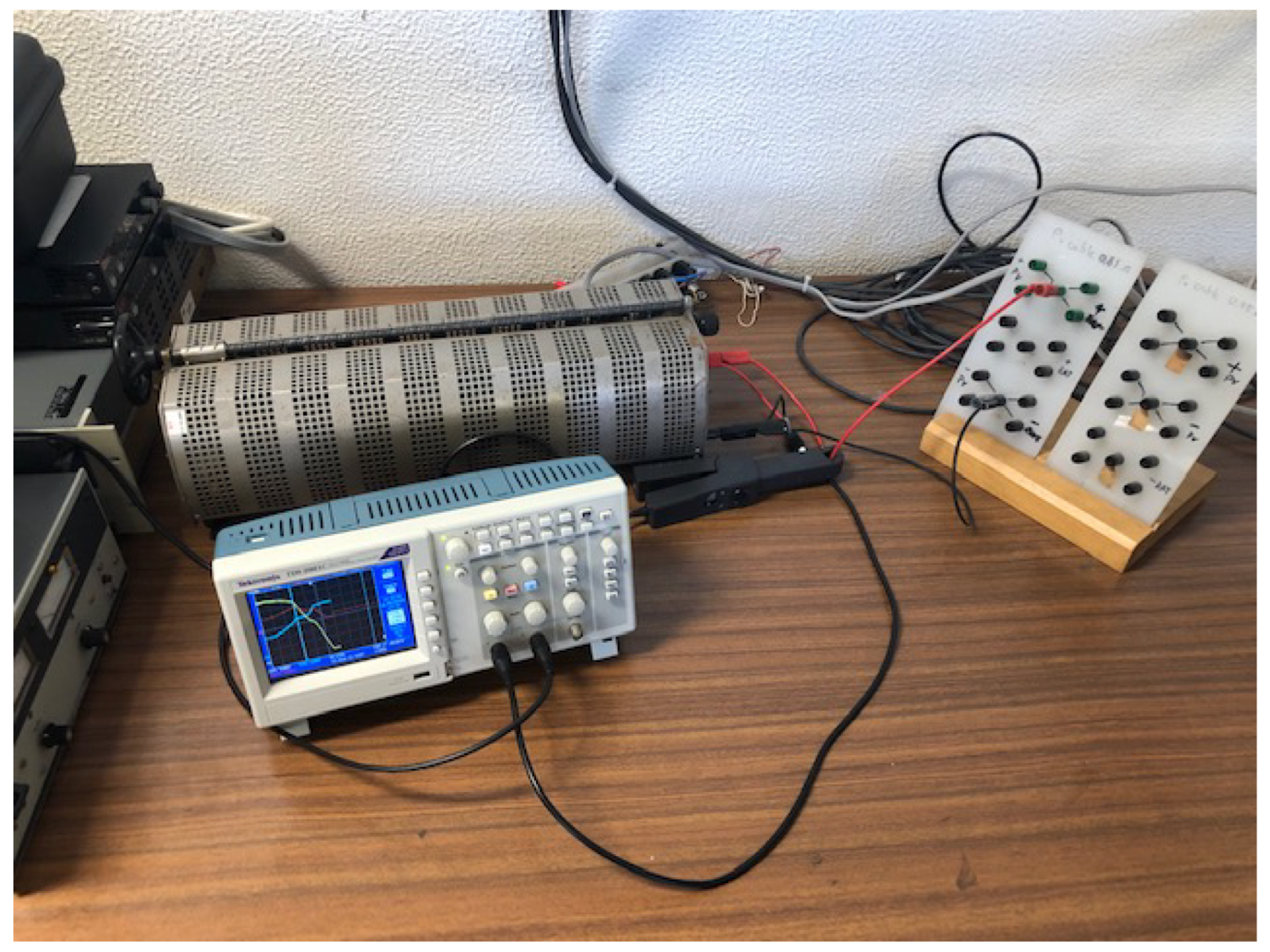
Figure 13.
Visualization of current, voltage, and power signals.


Table 1.
PERC and HJT STC parameters.
| Module | Max Rated Power [W] | Efficiency [%] | Temp. Coeff. [%/°C] |
|---|---|---|---|
| PERC | 395 | 20.2 | -0.350 |
| HJT | 370 | 20.6 | -0.259 |
Table 2.
Irradiance, module efficiency, temperature, and output power for August’s 18th.
| Time | Pout-HJT | Eff-HJT | Temp-HJT | Pout-PERC | Eff-PERC | Temp-PERC | Irradiance |
|---|---|---|---|---|---|---|---|
| 08:30 | 56,28 | 11,05 | 13,1 | 60,8 | 10,96 | 15 | 284 |
| 08:45 | 73,00 | 13,26 | 16,8 | 73,65 | 12,28 | 17,3 | 307 |
| 09:00 | 90,79 | 13,68 | 22,5 | 91,13 | 12,61 | 21,3 | 370 |
| 09:15 | 108,56 | 14,66 | 26,6 | 96,48 | 11,96 | 23,7 | 413 |
| 09:30 | 152,76 | 16,35 | 29,9 | 136,98 | 13,46 | 29,1 | 521 |
| 09:45 | 194,30 | 19,96 | 33,4 | 162,11 | 15,28 | 33,4 | 543 |
| 10:00 | 200,89 | 18,99 | 35,3 | 189,90 | 16,48 | 36,1 | 590 |
| 10:15 | 236,54 | 21,91 | 42,1 | 183,04 | 15,57 | 41,2 | 602 |
| 10:30 | 224,35 | 18,35 | 44,6 | 220,32 | 16,54 | 43,6 | 682 |
| 10:45 | 250,24 | 20,61 | 52,9 | 227,32 | 17,19 | 52 | 677 |
| 11:00 | 258,72 | 19,66 | 56,5 | 222,91 | 15,55 | 55,2 | 733,8 |
| 11:15 | 257,63 | 18,87 | 59,5 | 240,06 | 16,14 | 61,8 | 761,6 |
| 11:30 | 273,80 | 19,02 | 64,2 | 253,08 | 16,14 | 62,2 | 802,8 |
| 11:45 | 256,94 | 17,10 | 61,7 | 234,6 | 14,33 | 62,1 | 838 |
| 12:00 | 245,21 | 12,85 | 63,5 | 239,68 | 11,53 | 61 | 1064 |
| 12:15 | 258,56 | 16,00 | 66,2 | 239,56 | 13,61 | 64,8 | 901,2 |
| 12:30 | 248,86 | 13 | 68 | 241,82 | 11,6 | 66,7 | 1072 |
| 12:45 | 256,22 | 12,64 | 69,7 | 239,4 | 10,84 | 68 | 1130 |
| 13:00 | 261,12 | 11,10 | 68,7 | 248,6 | 9,70 | 66,6 | 1312 |
| 13:15 | 260,38 | 15,53 | 68,3 | 248,64 | 13,61 | 65,9 | 935,2 |
| 13:30 | 262,03 | 16,47 | 67,8 | 250,86 | 14,47 | 66,4 | 887,3 |
| 13:45 | 256,22 | 17,81 | 68,6 | 248,64 | 15,86 | 66,3 | 902,5 |
| 14:00 | 258,56 | 16,35 | 71,8 | 246,24 | 14,29 | 68,4 | 882 |
| 14:15 | 253,79 | 16,12 | 70,5 | 244,2 | 14,24 | 70,3 | 878,3 |
| 14:30 | 257,92 | 16,19 | 71 | 244,08 | 14,07 | 69,7 | 888,5 |
Table 3.
Irradiance, module efficiency, module temperature, and output power for August’s 19th.
| Time | Pout-HJT | Eff-HJT | Temp-HJT | Pout-PERC | Eff-PERC | Temp-PERC | Irradiance |
|---|---|---|---|---|---|---|---|
| 09:15 | 118,27 | 14,50 | 34,4 | 99,07 | 11,15 | 34,8 | 455 |
| 09:30 | 145,00 | 16,10 | 38,3 | 140,65 | 14,33 | 39,7 | 502,3 |
| 09:45 | 197,12 | 20,68 | 43,7 | 157,58 | 15,18 | 44,4 | 531,6 |
| 10:00 | 193,76 | 17,79 | 45,1 | 180,14 | 15,18 | 45,6 | 607,5 |
| 10:15 | 228,41 | 20,53 | 48,2 | 185,92 | 15,34 | 48,7 | 620,5 |
| 10:30 | 220,32 | 17,76 | 50,2 | 217,05 | 16,06 | 50,8 | 691,9 |
| 10:45 | 244,35 | 18,93 | 55,9 | 233,23 | 16,59 | 55,7 | 719,8 |
| 11:00 | 253,44 | 18,64 | 57,6 | 236,16 | 15,95 | 57,1 | 758,2 |
| 11:15 | 252,8 | 17,81 | 59,7 | 240,72 | 15,57 | 61,8 | 791,6 |
| 11:30 | 258,73 | 17,75 | 66,2 | 248,4 | 15,64 | 65,9 | 813,1 |
| 11:45 | 245,76 | 16,46 | 67,2 | 232,22 | 14,28 | 64,6 | 832,7 |
| 12:00 | 236,59 | 15,24 | 68,3 | 235,32 | 13,91 | 66,8 | 865,9 |
| 12:15 | 243,04 | 15,31 | 70,7 | 232,96 | 13,47 | 68,6 | 885,2 |
| 12:30 | 237,63 | 14,59 | 71 | 235,4 | 13,27 | 69,4 | 908,3 |
| 12:45 | 239,61 | 11,28 | 72,6 | 237,44 | 10,26 | 70 | 1185 |
| 13:00 | 242,11 | 14,72 | 73,6 | 239,68 | 13,38 | 71,2 | 917,2 |
| 13:15 | 248,68 | 15,08 | 75,8 | 239,4 | 13,33 | 73,6 | 919,6 |
| 13:30 | 243,2 | 15,49 | 76,9 | 237,12 | 13,86 | 75,3 | 875,5 |
| 13:45 | 244,8 | 15,51 | 76,6 | 237,3 | 13,80 | 76 | 880,3 |
| 14:00 | 239,18 | 14,90 | 77,1 | 233,2 | 13,34 | 76,2 | 895,2 |
| 14:15 | 238,33 | 15,29 | 78,1 | 231 | 13,61 | 75,3 | 869 |
| 14:30 | 240,76 | 15,65 | 78,1 | 232,96 | 13,90 | 76,7 | 857,7 |
Table 4.
Irradiance, module efficiency, temperature, and output power for August’s 25th.
| Time | Pout-HJT | Eff-HJT | Temp-HJT | Pout-PERC | Eff-PERC | Temp-PERC | Irradiance |
|---|---|---|---|---|---|---|---|
| 09:45 | 14,68 | 5,55 | 24,8 | 22,17 | 7,69 | 24,6 | 147,6 |
| 10:00 | 35,85 | 12,80 | 28,3 | 58,20 | 19,08 | 28,5 | 156,2 |
| 10:15 | 26,86 | 13,67 | 28,3 | 34,11 | 15,93 | 29,3 | 109,6 |
| 10:30 | 19,84 | 9,80 | 26,9 | 32 | 14,51 | 27,6 | 112,9 |
| 10:45 | 34,52 | 11,80 | 28,4 | 49,10 | 15,40 | 28,9 | 163,2 |
| 11:00 | 67,39 | 15,08 | 32,4 | 112,89 | 23,19 | 33,3 | 249,3 |
| 11:15 | 96,2 | 16,71 | 34,6 | 123,48 | 19,69 | 35,4 | 321,1 |
| 11:30 | 115,2 | 23,52 | 36,7 | 117,6 | 22,04 | 37,8 | 273,2 |
| 11:45 | 157,52 | 24,015 | 39,1 | 173,6 | 24,296 | 40,6 | 365,9 |
| 12:00 | 123,08 | 21,96 | 40,6 | 144 | 23,58 | 40,9 | 312,6 |
| 12:15 | 292,4 | 16,75 | 45,1 | 285,56 | 15,02 | 45 | 973,3 |
| 12:30 | 304,48 | 17,37 | 45,7 | 285,56 | 14,95 | 46 | 977,6 |
| 12:45 | 264 | 12,35 | 51,3 | 268,4 | 11,53 | 51,1 | 1192 |
| 13:00 | 272 | 12,70 | 49,7 | 264 | 11,32 | 48,3 | 1194 |
| 13:15 | 258,96 | 16,40 | 53,4 | 262,2 | 15,24 | 53,5 | 880,7 |
| 13:30 | 256,88 | 15,55 | 55,1 | 261,96 | 15,86 | 54,9 | 845,7 |
| 13:45 | 257,4 | 16,67 | 53 | 268,8 | 15,98 | 51,9 | 861,3 |
| 14:00 | 260,52 | 16,79 | 52,7 | 264 | 15,62 | 52,5 | 865,5 |
| 14:15 | 257,4 | 16,63 | 54 | 266,2 | 15,79 | 51,8 | 863,3 |
| 14:30 | 258,4 | 16,85 | 54,5 | 261,36 | 15,64 | 52,3 | 855,3 |
| 14:45 | 253,08 | 17,15 | 55,3 | 257,04 | 15,99 | 54,1 | 823,1 |
| 15:00 | 250,12 | 17,07 | 55,8 | 255,2 | 15,99 | 55,1 | 817,3 |
Table 5.
Irradiance, module efficiency, module temperature, and output power for August’s 29th.
| Time | Po-HJT | V-HJT | T-HJT | Po-PERC | V-PERC | T-PERC | Irr |
|---|---|---|---|---|---|---|---|
| 09:45 | 196,5 | 19,5 | / | 180,8 | 16,5 | / | 561,6 |
| 10:00 | 60,9 | 33,4 | / | 58,4 | 29,4 | / | 101,6 |
| 10:15 | 77,3 | 33,8 | / | 82,9 | 33,3 | / | 127,6 |
| 10:30 | 45,8 | 31,7 | / | 57,6 | 36,6 | / | 80,6 |
| 10:45 | 272,1 | 19,9 | 50,1 | 248,1 | 16,6 | 50,4 | 763,9 |
| 11:00 | 301,9 | 21,47 | 55,9 | 259,08 | 16,9 | 52,4 | 784,3 |
| 11:15 | 261,9 | 17,8 | 57,8 | 264,5 | 16,5 | 56 | 821,8 |
| 11:30 | 140,3 | 20,6 | 54,8 | 151,2 | 20,4 | 54,4 | 379,9 |
| 11:45 | 253,4 | 17,4 | 58,2 | 240,7 | 15,2 | 55,4 | 811,7 |
| 12:00 | 250,4 | 15,4 | 59,9 | 253,1 | 14,3 | 58,7 | 905,7 |
| 12:15 | 253,8 | 15,9 | 61 | 262,2 | 15,1 | 60,2 | 889,2 |
| 12:30 | 247,00 | 15,1 | 61,7 | 254,4 | 14,3 | 60,8 | 912,7 |
| 12:45 | 286,0 | 16,2 | 60,3 | 277,8 | 14,4 | 61,6 | 985,3 |
| 13:00 | 257,6 | 15,6 | 63,3 | 259,6 | 14,5 | 63,1 | 918,8 |
| 13:15 | 252,8 | 15,2 | 69,9 | 253,1 | 13,9 | 69,6 | 927,7 |
| 13:30 | 249,3 | 15,8 | 66 | 250,9 | 14,6 | 64,1 | 881,7 |
| 13:45 | 257,6 | 15,9 | 65,9 | 252,5 | 14,3 | 64,6 | 902,3 |
| 14:00 | 232,1 | 15,2 | 66,3 | 244,2 | 14,6 | 64,9 | 853,8 |
| 14:15 | 236,2 | 15,3 | 66 | 242 | 14,4 | 64,5 | 861,5 |
| 14:30 | 232,1 | 15,3 | 65,7 | 236,6 | 14,4 | 64,3 | 843,7 |
| 14:45 | 229,8 | 15,3 | 63,9 | 233,2 | 14,2 | 63,2 | 838,3 |
| 15:00 | 220,4 | 14,9 | 63,7 | 232,1 | 14,5 | 62,3 | 821,7 |
Table 6.
Daily and average efficiencies of the modules.
| Day | HJT Efficiency [%] | PERC Efficiency [%] |
|---|---|---|
| August’s 2th | 18,31 | 15,20 |
| August’s 18th | 16,31 | 13,94 |
| August’s 19th | 16,37 | 14,16 |
| August’s 25th | 16,02 | 14,91 |
| August’s 29th | 16,52 | 14,96 |
| Average | 16,51 | 14,63 |
Table 7.
Total energy conversion performed by the modules during one year.
| Month | Total Irradiance [] | HJT Output [] | PERC Output [] |
|---|---|---|---|
| January | 69,96 | 20,71 | 19,98 |
| February | 97,97 | 29,00 | 27,99 |
| March | 145,81 | 43,15 | 41,66 |
| April | 153,19 | 45,34 | 43,76 |
| May | 220,1 | 65,14 | 62,88 |
| June | 225,65 | 66,78 | 64,47 |
| July | 247,2 | 73,16 | 70,62 |
| August | 211,85 | 62,70 | 60,52 |
| September | 160,63 | 47,54 | 45,89 |
| October | 114,76 | 33,96 | 32,79 |
| November | 67,25 | 19,90 | 19,21 |
| December | 64,78 | 19,17 | 18,51 |
| Total | 1779,15 | 526,56 | 508,28 |
Table 8.
Energy suppliers in Portugal and their tariffs for 2022.
| Suppliers | [€] |
|---|---|
| EDP commercial | 0,2377 |
| Goldenergy | 0,1465 |
| Endesa | 0,1449 |
| Iberdrola | 0,1491 |
| Galp Energia | 0,243 |
Table 9.
Average power delivered by each module for each month.
| Month | Power HJT [W] | Power PERC [W] |
|---|---|---|
| January | 83,49 | 80,59 |
| February | 129,44 | 124,95 |
| March | 174,01 | 167,97 |
| April | 188,90 | 182,35 |
| May | 262,66 | 253,54 |
| June | 278,26 | 268,60 |
| July | 295,00 | 284,76 |
| August | 252,81 | 244,04 |
| September | 198,08 | 191,20 |
| October | 136,95 | 132,19 |
| November | 82,93 | 80,05 |
| December | 77,30 | 74,62 |
Table 10.
Average monthly system power divided by inverter nominal power.
| Month | Power HJT [%] | Power PERC [%] |
|---|---|---|
| January | 27,13 | 27,63 |
| February | 42,07 | 42,84 |
| March | 56,55 | 57,59 |
| April | 61,40 | 62,52 |
| May | 85,37 | 86,93 |
| June | 90,44 | 92,09 |
| July | 95,88 | 97,63 |
| August | 82,17 | 83,67 |
| September | 64,38 | 65,56 |
| October | 44,51 | 45,33 |
| November | 26,95 | 27,45 |
| December | 25,12 | 25,59 |
Table 11.
Inverters efficiencies related to primary power and module technology.
| Efficiency | Efficiency for HJT [%] | Efficiency for PERC [%] |
|---|---|---|
| at 25% of | 95,50 | 95,13 |
| at 30% of | 96,00 | 95,67 |
| at 50% of | 96,80 | 96,67 |
| at 75% of | 97,17 | 97,07 |
Table 12.
Monthly inverter efficiencies.
| Month | HJT Inverter Efficiency [%] | PERC Inverter Efficiency [%] |
|---|---|---|
| January | 95,50 | 95,13 |
| February | 96,00 | 95,67 |
| March | 96,80 | 96,67 |
| April | 96,80 | 96,67 |
| May | 97,17 | 97,07 |
| June | 97,17 | 97,07 |
| July | 97,17 | 97,07 |
| August | 97,17 | 97,07 |
| September | 96,80 | 96,67 |
| October | 96,00 | 95,67 |
| November | 95,50 | 95,13 |
| December | 95,50 | 95,13 |
Table 13.
Monthly and yearly energy produced by 13 HJT and 12 PERC modules.
| Month | Energy Produced HJT [kWh] | Energy Produced PERC [kWh] |
|---|---|---|
| January | 257,06 | 228,17 |
| February | 361,86 | 321,31 |
| March | 543,05 | 483,21 |
| April | 570,53 | 507,67 |
| May | 822,83 | 732,42 |
| June | 843,58 | 750,89 |
| July | 924,14 | 822,60 |
| August | 791,99 | 704,97 |
| September | 598,24 | 532,32 |
| October | 423,87 | 376,38 |
| November | 247,10 | 219,33 |
| December | 238,02 | 211,27 |
| Annual | 6622,28 | 5890,55 |
Table 14.
Annual revenue of HJT and PERC system accounting for module degradation for 30 years.
| Year | HJT [€] | PERC [€] | Year | HJT [€] | PERC [€] | Year | HJT [€] | PERC [€] |
|---|---|---|---|---|---|---|---|---|
| 1 | 1217,65 | 1079,33 | 11 | 1193,57 | 1021,73 | 21 | 1162,98 | 967,20 |
| 2 | 1215,22 | 1073,43 | 12 | 1191,18 | 1016,14 | 22 | 1160,66 | 961,90 |
| 3 | 1212,80 | 1067,56 | 13 | 1188,81 | 1010,58 | 23 | 1158,34 | 956,64 |
| 4 | 1210,38 | 1061,72 | 14 | 1186,43 | 1005,05 | 24 | 1156,03 | 951,41 |
| 5 | 1207,96 | 1055,91 | 15 | 1184,07 | 999,55 | 25 | 1153,72 | 946,21 |
| 6 | 1205,55 | 1050,14 | 16 | 1181,70 | 994,09 | 26 | 1151,42 | 941,03 |
| 7 | 1203,14 | 1044,39 | 17 | 1175,82 | 988,65 | 27 | 1149,12 | 935,88 |
| 8 | 1200,74 | 1038,68 | 18 | 1173,48 | 983,24 | 28 | 1146,83 | 930,76 |
| 9 | 1198,35 | 1033,00 | 19 | 1167,64 | 977,86 | 29 | 1144,54 | 925,67 |
| 10 | 1195,95 | 1027,35 | 20 | 1165,31 | 972,51 | 30 | 1142,26 | 920,61 |
Table 15.
Cumulative revenues of systems using both technologies for 12,15,20 and 30 years.
| Time [years] | Revenues HJT [€] | Revenues PERC [€] | Revenue Difference [€] |
|---|---|---|---|
| 12 years | 14452,50 | 12569,36 | 1883,14 |
| 15 years | 18011,81 | 15584,55 | 2427,26 |
| 20 years | 23875,76 | 20500,91 | 3374,85 |
| 30 years | 35401,68 | 29938,23 | 5463,45 |
Table 16.
HJT and PERC system costs for 4,5 kW system.
| Material | HJT [€] | PERC [€] |
|---|---|---|
| Modules | 3528,01 | 1849.92 |
| Inverters | 1389,00 | 1314,99 |
| Cables | 280 | 280 |
| Structure | 781,82 | 781,82 |
| Labour | 1000 | 1000 |
| Total | 6978,83 | 5226,73 |
Table 17.
Cumulative, APpY and AROI for 10,12,15,20 and 30 years- 4,5 kW installation.
| Years | HJT Revenue [€] | PERC Revenue [€] | APpY HJT [€] | APpY PERC [€] | AROI HJT [%] | AROI PERC [%] |
|---|---|---|---|---|---|---|
| 10 | 5088,97 | 5304,77 | 508,90 | 530,48 | 7,29 | 10,15 |
| 12 | 7473,68 | 7342,64 | 622,81 | 611,89 | 8,92 | 11,7 |
| 15 | 11032,99 | 10357,82 | 735,53 | 690,52 | 10,54 | 13,21 |
| 20 | 16896,94 | 15274,18 | 844,85 | 763,71 | 12,1 | 14,61 |
| 30 | 28422,85 | 24711,51 | 947,43 | 823,72 | 13,58 | 15,76 |
Table 18.
HJT and PERC system costs for 3,5 kW system.
| Material | HJT [€] | PERC [€] |
|---|---|---|
| Modules | 2713,85 | 1387,44 |
| Inverters | 1389,00 | 1314,99 |
| Cables | 280 | 280 |
| Structure | 781,82 | 781,82 |
| Labour | 1000 | 1000 |
| Total | 6164,67 | 4764,25 |
Table 19.
Cumulative, APpY and AROI for 10,12,15,20 and 30 years- 3.5 kW installation.
| Years | HJT Revenue [€] | PERC Revenue [€] | APpY HJT [€] | APpY PERC [€] | AROI HJT [%] | AROI PERC [%] |
|---|---|---|---|---|---|---|
| 10 | 3118,22 | 3134,38 | 311,82 | 313,44 | 5,06 | 6,58 |
| 12 | 4952,64 | 4662,78 | 412,72 | 388,56 | 6,70 | 8,16 |
| 15 | 7690,57 | 6924,17 | 512,71 | 461,61 | 8,32 | 9,69 |
| 20 | 12201,31 | 10611,43 | 610,07 | 530,57 | 9,90 | 11,14 |
| 30 | 21067,39 | 17689,43 | 702,25 | 589,65 | 11,39 | 12,38 |
Table 20.
HJT and PERC system costs for 2.5 kW system.
| Material | HJT [€] | PERC [€] |
|---|---|---|
| Modules | 1899,70 | 1079,12 |
| Inverters | 1389,00 | 1314,99 |
| Cables | 280 | 280 |
| Structure | 781,82 | 781,82 |
| Labour | 1000 | 1000 |
| Total | 5350,52 | 4455,93 |
Table 21.
Cumulative, APpY and AROI for 10,12,15,20 and 30 years- 2.5 kW installation.
| Years | HJT Profit [€] | PERC Profit [€] | APpY HJT [€] | APpY PERC [€] | AROI HJT [%] | AROI PERC [%] |
|---|---|---|---|---|---|---|
| 10 | 1147,51 | 1687,45 | 114,75 | 168,75 | 2,14 | 3,79 |
| 12 | 2431,61 | 2876,20 | 202,63 | 235,6 | 3,79 | 5,29 |
| 15 | 4348,16 | 4635,06 | 289,88 | 309,00 | 5,42 | 6,93 |
| 20 | 7505,67 | 7502,94 | 375,28 | 375,15 | 7,01 | 8,42 |
| 30 | 13711,93 | 13008,04 | 457,06 | 433,60 | 8,54 | 9,73 |
Table 22.
HJT and PERC system costs for 5000 € installations.
| Material | HJT [€] | PERC [€] |
|---|---|---|
| Modules | 1356,93 | 1541,6 |
| Inverters | 1389,00 | 1314,99 |
| Cables | 280 | 280 |
| Structure | 781,82 | 781,82 |
| Labour | 1000 | 1000 |
| Total | 4807,75 | 4918,41 |
Table 23.
Cumulative, APpY and AROI for 10,12,15,20 and 30 years- 5000€ installation.
| Years | HJT Profit [€] | PERC Profit [€] | APpY HJT [€] | APpY PERC [€] | AROI HJT [%] | AROI PERC [%] |
|---|---|---|---|---|---|---|
| 10 | -166,30 | 3857,84 | -16,63 | 385,78 | -0,35 | 7,84 |
| 12 | 750,91 | 5556,06 | 62,58 | 463,00 | 1,30 | 9,41 |
| 15 | 2119,88 | 8068,72 | 141,33 | 537,91 | 2,94 | 10,94 |
| 20 | 4375,24 | 12165,68 | 218,76 | 608,28 | 4,55 | 12,37 |
| 30 | 8808,29 | 20030,12 | 293,61 | 667,67 | 6,11 | 13,57 |
Table 24.
HJT and PERC system costs for 10000€ installations.
| Material | HJT [€] | PERC [€] |
|---|---|---|
| Modules | 4613,55 | 3854 |
| Inverters | 1690 | 1970 |
| Cables | 420 | 560 |
| Structure | 1563,64 | 1563,64 |
| Labour | 1500 | 2000 |
| Total | 9787,19 | 9947,64 |
Table 25.
Cumulative, APpY and AROI for 10, 12, 15, 20 and 30 years- 10000 € installation.
| Years | HJT Profit [€] | PERC Profit [€] | APpY HJT [€] | APpY PERC [€] | AROI HJT [%] | AROI PERC [%] |
|---|---|---|---|---|---|---|
| 10 | 6922,02 | 19013,99 | 692,20 | 1901,40 | 7,07 | 19,11 |
| 12 | 10223,98 | 24618,12 | 852,00 | 2051,51 | 8,71 | 20,62 |
| 15 | 15152,25 | 32909,89 | 1010,15 | 2194,00 | 10,3 | 22,01 |
| 20 | 23271,57 | 46429,87 | 1163,58 | 2321,49 | 11,89 | 23,33 |
| 30 | 39230,53 | 72382,51 | 1307,68 | 2412,75 | 13,36 | 24,25 |
Disclaimer/Publisher’s Note: The statements, opinions and data contained in all publications are solely those of the individual author(s) and contributor(s) and not of MDPI and/or the editor(s). MDPI and/or the editor(s) disclaim responsibility for any injury to people or property resulting from any ideas, methods, instructions or products referred to in the content. |
© 2024 by the authors. Licensee MDPI, Basel, Switzerland. This article is an open access article distributed under the terms and conditions of the Creative Commons Attribution (CC BY) license (https://creativecommons.org/licenses/by/4.0/).
Copyright: This open access article is published under a Creative Commons CC BY 4.0 license, which permit the free download, distribution, and reuse, provided that the author and preprint are cited in any reuse.


