
Submitted:
08 October 2024
Posted:
10 October 2024
You are already at the latest version
Abstract
The new PV technologies, such as bifacial modules, brings the challenge of analyzing the response of numerical models and their fit to actual measurements. Thus, this study explores various models available in the literature for simulating the IV curve behavior of bifacial photovoltaic modules. The analysis contains traditional models, such as single and double-diode models, and empirical or analytical methodologies. Therefore, this paper proposes and implements a model performance assessment framework. This framework aims to establish a common basis for comparison and verify the applicability of each model by contrasting it with experimental data under controlled conditions of irradiance and temperature.
The study utilizes bifacial modules of PERC+, HJT, and n-PERT technologies, tracing IV curves using a high-precision A+A+A+ solar simulator and conducting two sets of laboratory illumination easurements: single-sided and double-sided. In the first case, each face of the module is illuminated separately, while in the latter, the incident frontal illuminating light is reflected on a reflective surface. Experimental data obtained from these measurements are used to evaluate three different approximations for bifacial IV curve models in the case of double-sided illumination. The employed model for single-sided illumination is a single-diode model. The evaluation of various models revealed that shadowing from frames and junction boxes contributes to an increase in the error of modeled IV curves.
However, among the three evaluated bifacial electrical models, one exhibited superior performance, with current errors approaching approximately 20%. To mitigate this discrepancy, a proposed methodology highlighted the significance of accurately estimating Io, suggesting its potential to reduce errors.
Keywords:
n/a
; PV models
; bifacial module
; experimental data
1. Introduction
Bifacial photovoltaic (PV) technology, in contrast to its monofacial counterparts, offers the unique capability of harnessing solar energy from both the front and rear sides of the PV module. This technology increased significance and is projected to capture a substantial 70% market share by 2030 [1]. The advantages of adopting bifacial PV technology over monofacial systems are diverse and compelling. First, the ability to capture light from both sides leads to notable gains in energy production [2,3,4]. Bifacial PV systems exhibit enhanced energy yield by leveraging reflected light from the ground, surrounding surfaces, and even the sky. Second, the deployment of bifacial modules, even with a simple arrangement, contributes to a reduction in the levelized cost of energy. However, this cost reduction can be further optimized by utilizing increased albedo, emphasizing the importance of considering the reflective properties of the installation area [5]. Last, bifacial PV technology demonstrates its value of climate change since it could offer higher power outputs for future irradiance scenarios than monofacial PV, making them a promising choice for sustainable energy generation [6]. In this scenario, it is important to have reliable tools that can accurately predict the energy production of PV modules or arrangements under different environmental conditions. Since different locations have their unique temperature levels, irradiance, humidity, and other factors, it is essential to consider these variables when modeling energy production. For that purpose, several electrical, thermal, and optical models have been developed to represent the behavior of PV devices. Considering that bifacial PV technology is relatively new, it is necessary to conduct more research to determine if current models are good enough to represent its behavior or if new modeling approaches are required to lead to more accurate predictions of energy production.
The electrical output of a PV device can be simulated using diverse models. One commonly employed approach is based on the single diode formulation [7,8,9,10,11,12], which incorporates five parameters: photocurrent (), diode ideality factor (), diode saturation current (), series resistance (), and shunt resistance () [13]. However, as the single-diode model inherently assumes a monofacial setup, adjustments are required to accommodate the contribution of both faces of a bifacial device. The initial approximation to transform the monofacial model into a bifacial representation involves introducing an equivalent . This equivalent current is derived from the combination of front and rear irradiances [14,15,17]. An alternative representation proposed in [13,15] for bifacial devices involves adapting the single diode model by connecting two circuits in parallel. In this configuration, one branch represents the frontal face with its respective parameters. In contrast, the other branch represents the rear. The addition of the currents generated in both branches yields . Studies have indicated that the configuration utilizing the equivalent current source exhibits superior performance compared to the parallel configuration [15]. In certain cases, the single-diode model has been further simplified by disregarding resistive effects and eliminating series and shunt resistances [18]. Another formulation extensively used for monofacial PV devices is the double diode model [19,20], which has also been adapted to analyze of bifacial PV devices. This model has demonstrated remarkable accuracy under standard test conditions (STC) and in various temperature and irradiance conditions [21,22]. The topology of the model closely resembles that of the single-diode model, with an additional diode included in parallel. Incorporating an additional diode into the two-diode model introduces two new parameters, resulting in a formulation with seven parameters. These parameters include photocurrent (), diode ideality factors (, ), diode saturation currents (, ), series resistance (), and shunt resistance (). Some authors have applied this formulation to bifacial PV devices [14,15]. Other formulations beyond the single and double diode models have been proposed. In [16], two monofacial electrical models are utilized. The first is an analytical model proposed by Eduardo et al. [26], while the second is an empirical model proposed by King et al. [27]. Both models demonstrated effective performance for non-real-time monitoring, particularly in clear sky conditions, with the analytical model exhibiting greater accuracy compared to the empirical model.
In fact, several electrical models have been proposed to represent the behavior of bifacial PV modules. Table 1 offers a comprehensive overview of how these models have been validated. Outdoor measurements emerge as the primary method utilized. However, some studies employ simulations to delve into specific aspects or scenarios. While validation methods predominantly rely on energy output and power to compare model and experimental results, the analysis of the IV curve is equally crucial. It provides valuable insights into the fit of the selected parameters and reveals any disparities between experimental data and the proposed model. In summary, the validation of the proposed electrical model to represent bifacial technology have relied on outdoor data or simulations, which may lack the control necessary for robust analysis. The limitations of outdoor measurements, such as less control over irradiance distribution and module temperature, underscore the necessity for alternative validation methods.
This article assesses existing electrical models for bifacial PV technology by utilizing high-quality data obtained in an indoor solar simulator. By conducting evaluations in a controlled environment, this research seeks to provide a comprehensive understanding of the performance of various electrical models for bifacial PV modules based on an accurate and reliable assessments. The high-quality experimental data consists in a set of IV curve of several PV modules of different manufacturers and technologies under controlled irradiance and temperature conditions, which are obtained in a A+A+A+ Eternalsun sun simulator. Controlled conditions of irradiance are very important since the PV modules are sensitive to spectral distribution of solar irradiance [7], and specifically, the presence of clouds difficult its prediction [8]. Having a controlled ambient helps to avoid the errors coming from the optical model and the different noise sources related to clouds, reflections, and shadowing.

Table 1.
Proposed validation methods.
| Validation method |
Ref | Proposed model |
Evaluation method |
PV device | Technology | Measurement conditions |
|---|---|---|---|---|---|---|
| Outdoor measurement |
[13] | Parallel single diode |
IV curve | Cell | Not reported | Temperature: 25-55°C. Irradiance: 1000 W/m2. |
| Module | Not reported | Albedo: 0.16. Irradiance: 900 ± 20 W/m2. |
||||
| Outdoor measurement |
[14] | Double diode | Annual bifacial gain and energy output |
Cell | N-type | Vertical east-west orientation. Two different albedo. |
| Outdoor measurement |
[15] | Single and double diode |
IV curve | Module | N-type | Frontal irradiance at 1000 W/m2 while rear irradiance varies between 0% and 30%. |
| Outdoor measurement |
[15] | Single diode traditional and parallel configuration |
Power and cumulative energy |
Module | Not reported | Daily performance estimation, considering summer and winter days. |
| Outdoor measurement |
[16] | Analytical and empirical |
DC power | Monofacial and bifacial PV array |
PERC | Variation in albedo levels Different levels of temperature and irradiance depending on weather conditions. |
| Simulation | [17] | Single diode | Energy yield | Module | Not reported | Daily and yearly performance estimation, considering sunny and cloudy days. |
| Simulation | [18] | Single diode | IV curves for monofacial and bifacial module |
Module | Not reported | STC condition: 25°C and 1000 W/m2. 20°C and 800 W/m2. |
This research seeks to identify the most accurate electrical model for bifacial PV technology. By comparing the simulated results of different models against meticulously collected indoor data, the research aims to discern which model best captures the complex behavior of bifacial modules. Additionally, the study aims to assess the sensitivity of the best electrical models to variations in electrical parameters, providing insights into the factors that significantly impact model accuracy. This study is structured into several key sections. It begins with a concise review of the indoor characterization of bifacial PV devices, followed by an examination of proposed bifacial models found in existing literature. The methodology section provides a detailed exposition of the experimental setup and the associated data processing methodologies. Subsequent sections present the results obtained from both single-sided and double-sided measurements. Finally, the study culminates with comprehensive conclusions drawn from the synthesis of gathered data and the analyses conducted throughout the investigation.
2. Characterization of Bifacial PV Devices
Characterization of PV devices provides relevant information regarding their performance, including max power rating, efficiency, estimation of annual energy yield, sizing of system components, and determination of product value [9]. Standard IEC 60904-1-2 [10] provides recommended electrical parameters for reporting and the corresponding measurement methods for bifacial PV devices. This overview will center on two types of illumination: single and double-sided. Specifically, the emphasis will be on indoor measurements, focusing on laboratory tests.
2.1. Single-Sided Illumination
When measuring IV curves on bifacial devices, one consideration is to illuminate only one side. The standard IEC 60904-1-2 specifies that the limit of irradiance on the non-illuminated side should be less than 3 Wm−2. There are multiple methods available to achieve this requirement:
- Use a non-reflective material behind the non-illuminate side.
- Limit the exposure of the module illuminating with a source of the size of the module.
- Cover the non-illuminated side with a black surface.
Liang et al. [11] investigated the considerations outlined in the standard and devised an experimental setup comprising two distinct darkrooms. They aimed to generate varying background reflections to examine their impact on characterization results. Their findings revealed that the non-uniformity of irradiance influences two parameters: fill factor and maximum power. Moreover, irradiances exceeding 3 Wm−2 were found to introduce uncertainties to the maximum power measurements. It is important to carefully consider the conditions under which the rear surface is exposed during single-sided characterization to minimize the effects of reflections and non-uniform irradiance. Implementing the recommended methods from the standard is crucial in addressing these issues. Razongles et al. [12] examined parasitic reflections occurring when the bifacial module is positioned away from the black screen surface to mitigate the effects above. They suggested placing a black screen directly on the back of the module to minimize reflections.
2.2. Double-Sided Illumination
In the case of double-sided illumination, it is crucial to accurately measure both frontal and rear irradiances and develop a method to illuminate both faces consistently. There are various arrangements and measurement techniques. For instance, Lagunas et al. [19] utilized a 10ms pulse class-A flash simulator to illuminate the device, with two glasses and mirrors positioned at a 45° tilt from the direction of the light pulse. A mesh was employed to control rear face light. Irradiance was measured using a reference cell, while current and voltage were gauged using probes. This setup enabled distinct irradiance levels on each side of the PV device. Different scenarios were examined to compare the IV curve behavior when the device was illuminated separately from each side or simultaneously. Results revealed that simultaneous illumination from both sides led to a lower maximum power point than the sum of currents obtained under separate illumination conditions.
Zhang et al. [20] comprehensively compared one-sided and two-sided illumination. Their experimental setup involved a light source directed towards a bifacial cell, and a white smooth plate capable of reflecting incident light. The same configuration was used for single-sided measurements, albeit with adjustments made to the distance between the laminates and the light source. They evaluated three different types of bifacial cells: n-type, p-type, and HJT. In contrast to the findings of Lagunas et al., they observed that two-sided illumination resulted in higher levels of maximum power points than to one-sided illumination.
Finally, Razongles et al. [12] implemented two indoor setups. The first is implemented for large modules, where two identical Eternal Sun sun simulators were ubicated at each device surface. With this configuration the irradiance can be totally controlled for both surfaces. The second setup utilized an aluminum-mirror arrangement specifically designed for 4-cell modules. This setup is very similar to the proposal of Lagunas et al., using a mesh as a filter to control the irradiance on the rear face.
Across the various presented setups, several commonalities emerge. Firstly, each setup utilizes reference cells to measure irradiances accurately. Additionally, there is a consistent practice of attenuating incident light on the rear face of the setup, emulating the albedo effect. These methodological consistencies serve as foundational pillars for the forthcoming exposition of our proposed setup, to be detailed in the Methodology section.
3. Bifacial Electrical Models
Previously, various models were discussed to elucidate the approaches adopted by different authors representing the electrical characteristics of bifacial PV modules. Among these models, the single-diode model (SDM) stands as a conventional choice. It is depicted in Equation(1), where the current sources symbolize both the frontal and rear sides of the bifacial module. Figure 1 shows a schematic representation of this model.
An alternative representation of the single diode model employs two parallel branches, each corresponding to one side of the module. This configuration is illustrated in Figure 2. The resultant current, denotated by in Equation (2) is the sum of Equation (3) and Equation (4).
Another commonly employed model is the double-diode model (DDM), as depicted in Equation (5). This formulation introduces an additional diode-current, necessitating the inclusion of two additional terms for and n. A visual representation is found in Figure 3.
3.1. The Bifacial Representation
As previously discussed, various models derive the IV curve and energy production for bifacial PV devices. Regardless of the specific model used, a crucial consideration lies in how these models effectively represent the bifacial nature of the device. Following parameter estimation, decisions must be made regarding each element in the circuit. In the work of [14], for instance, they proposed rescaling the parameters , , , and for both the front and rear faces while neglecting . This rescaling process is accomplished by incorporating the respective frontal and rear irradiances, as shown in Equations (6) and (7).
Where the term X represents , , and . It is important to note that is not a parameter found in datasheets. Furthermore, calculating , , and requires data for the rear face, which can be obtained from measurements.
In [15], both single and double-diode models were implemented. For parameter calculation, they conducted a two-stage optimization process. The current source is determined using the bifaciality factor (), as shown in Equation (8):
Subsequently, a new series resistance, denoted as , is introduced to , resulting in a combined series term of . The mathematical representation of the single-diode model is depicted in Equation (9). To incorporate the double-diode model, it simply needs to add the term corresponding to the second diode.
In other studies, such as [17], a single-diode model is implemented by considering only the frontal face parameters. As given by Equation (10), the adjustments for bifacial representation involve rescaling the irradiances for the term when parameter extraction is performed under non-STC conditions.
Here, is the equivalent irradiance obtained from Equation (11).
The subscript “ref” refers to standard test conditions (STC), represents the temperature coefficient for , and denotes the bifaciality factor.
In the case of [16], the bifacial behavior is quantified by the “bifacial gain of irradiance”, defined in Equation (12).
Notably, the authors applied the model to outdoor experimental data, hence the usage of , representing the irradiance in the plane of the array, and , indicating the loss of power due to non-homogeneity in the rear irradiance.
3.2. Models Evaluation
After reviewing the presented models and their respective validations, three have been chosen for a comprehensive evaluation of their performance using experimental data under controlled irradiance and stable temperature conditions. The selection criteria are based on their replicability and the diverse modeling approaches employed. The chosen models are as follows:
- Guet al. [17] The single-diode model requires 5 parameters. The estimation method the authors proposed for these parameters is implemented as described by Equations (13)–(17).Once the 5 parameters are calculated, they are adjusted to their actual irradiance and temperature conditions. The photocurrent () is defined in Equation (10), while the remaining parameters are computed using equations Equations (18)–(21):
- Janssenet al. [14] Utilizes a double-diode model, where initially 7 parameters have to be estimated. However, based on the author’s considerations, 3 parameters are assumed: , and . Then, to obtain the first diode saturation current, the formulation proposed by [21] is employed, given by Equation (22).On the other hand, the second diode saturation current is calculated by Equation (23).Finally, the series resistance is calculated by Equation (19) and are transformed to its original ambient conditions, the first is done by applying Equation (6), and the second is accomplished by the application of Equation (24).
- Bhanget al. [13] Proposed a single-diode model with a parallel configuration, resulting in the estimation of 10 parameters, 5 for the frontal face and the other 5 for the rear. A W-Lambert parameter estimation is employed to obtain it, utilizing the measured values at STC for both faces. Finally, the parameters are corrected utilizing Equation (10),Equation (18),Equation (19),Equation (20).
4. Methodology
4.1. Setup
This section describes the equipment utilized for measurements, beginning with PV bifacial modules and then proceeding to the sun simulator.
4.1.1. Bifacial Modules
Table 2 displays the various modules subjected to measurement. Different technologies were employed, with a predominant use of PERC+ and HJT. The last column indicates the specific test to be conducted, which will be elucidated in the subsequent sections. It is worth mentioning that GOPV PSDA6, HET GO 25 and n-PERT modules are frameless, whereas Risen, Trina, and SunPower modules are equipped with frames.
4.1.2. Solar Simulator
The Eternalsun sun simulator (A+A+A+ class) is employed to illuminate and trace IV curves for the selected modules. The sun simulator utilizes a single long-pulse filtered xenon tube lamp in the bottom chamber. Consequently, the module and reference cell must be oriented towards the bottom to receive the light. The irradiance levels can be controlled within 100 to 1200 Wm−2.
The upper chamber is mobile, allowing it to be lowered to cover the module completely, preventing the entry of external light. The interior of the upper chamber is black, eliminating any reflection of the emitted light. Once the upper chamber is lowered, temperature control is possible within a range of 10 to 75°C.
A reference cell is connected to measure irradiance, and within the interior of the bottom chamber, there is another cell named the “monitor cell”, which measures both irradiance and temperature.
Temperature measurement employs two instruments: the first utilizes four T-type thermocouples, primarily when tracing IV curves at different temperatures, as it allows temperatures above 100°C. The second is an IR thermal sensor, allowing temperature measurements up to approximately 49°C.
4.2. Measurement
The following sections describe the two tests conducted, the first one using single-sided illumination and the second one with double-sided illumination.
4.2.1. Single-Sided Illumination (SS)
4.2.2. Double-Sided Illumination (DS)
For this measurement, a 90% reflective film is employed to cover the surface of the upper chamber. This arrangement allows for the light emitted from the bottom to be partially reflected by this surface, thereby illuminating the rear face of the bifacial module.
As the reflected light onto the rear surface is not uniform, it becomes crucial to measure the irradiance across the surface of the modules. The modules were virtually divided into nine sections, marked by the red X symbols in Figure 6. The resulting irradiance distributions are named “irradiance matrix”. Irradiance measurements were conducted with a reference cell positioned in each section. Additionally, an extra point is included below position 2C, which is the reference cell’s position after irradiance measurement. This adjustment helps prevent shadowing on the rear face during IV curve tracing.
With this configuration, the upper chamber remains lifted to maintain reflection onto the surface. In this case, temperature cannot be controlled. However, frontal irradiance can also be regulated, affecting the rear irradiance. The module is exposed to irradiances ranging from 100 to 1000 Wm−2, in 100 Wm−2 increments. For every data point, the rear irradiance is measured in the position below 2C.
4.3. Data Processing and Model Approach
The processing will be divided into two parts, each corresponding to a different test. Among the seven models listed in Table 1, three have been chosen for their replicability, a selection process that will be detailed further below.
4.3.1. Single-Sided Illumination Measurement (SS)
In this measurement, the frontal and rear faces are tested to obtain their respective IV curves for STC conditions. It is important to note that the bifacial models previously discussed cannot be applied here, as two IV curves are traced separately. The primary objective of this test is to examine the behavior of each module face independently and to observe any potential differences between them.
In this scenario, the single-diode model is applied to analyze each IV curve. The standard test condition (STC) measured points (, , , and ) are employed for both the frontal and rear faces. Subsequently, these data points are inputted into the 5-parameter model for each face of the module. Following parameter acquisition, the models are used to simulate the IV curves. The comparison between the simulated and experimental IV curves involves calculating percent errors for voltage values, considering for current and for power. Figure 7 summarizes every step of this measurement.
4.3.2. Double-Sided Illumination Measurement (DS)
In this case the measured irradiances in Figure 6 are used to determine the minimum irradiance value under the assumption that this value limits the short-circuit current, given that each cell operates as a miniature current source [22]. This minimum value, along with the STC measured points, serves as input for evaluating the proposed models by [13,14,17].
Once the irradiances are measured, the reference cell is located under the 2C position, and IV curves are traced in the range from 100 to 1000 Wm−2 for the frontal side. The data used for evaluating the models is the STC data corresponding to , , , and , previously obtained by the single-sided illumination measurement.
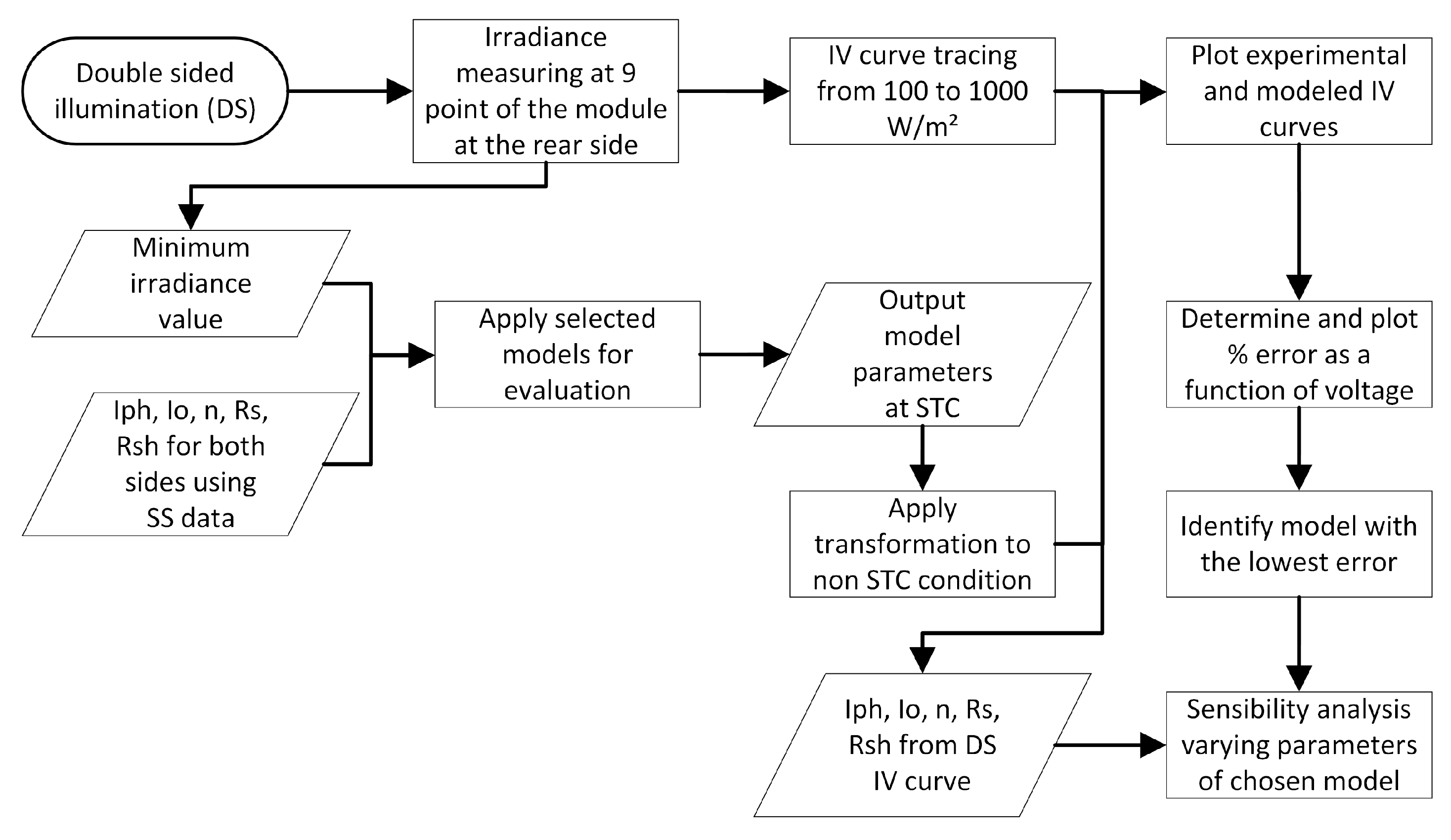
Figure 8.
Double-sided illumination measurement explanation scheme.
Analogous to SS measurements, percent errors are calculated by comparing experimental and modeled data to ascertain the model with the best performance. Once this model is identified, it undergoes comparison with direct parameter extraction using IV curves under DS illumination. Subsequently, a sensitivity evaluation is conducted to determine which parameters have the most significant impact on IV curve tracing.
5. Results and Discussion
The results are divided into two sections: single-sided and double-sided measurements. The best model from the double-sided measurements is then chosen for further parameter evaluation.
5.1. Single-Sided Illumination Measurement
IV curves for the five modules under STC conditions are modeled with SDM and contrasted with experimental data. Figure 9a, Figure 10a, Figure 11a, Figure 12a, Figure 13a display both frontal and rear IV curves for each module, while Figure 9b, Figure 10b, Figure 11b, Figure 12b, Figure 13b illustrate the differences between the estimated and measured values across the complete IV curve. These differences are particularly pronounced near the maximum power point. The module which presents the most appreciable differences between estimated and modeled current is SunPower, reaching a percentage error close to on the rear side, while the smaller differences are found in HET GO 25, with a maximum error in its rear side slightly superior to .
When the rear side is illuminated at 1000 Wm−2, the shadowing effect caused by the frames becomes apparent. This effect manifests as steps in the IV curve, leading to corresponding steps in the difference between the model and experimental data. In certain instances, such as with the SunPower module, additional shadowing occurs due to the connection box, leading to more pronounced steps along the IV curve and a significant disparity near the maximum power point. This effect could explain the behavior detailed previously, when the rear side reached the maximum differences. While this behavior may not significantly affect maximum power estimation in tilted configurations, it could pose challenges in vertical east-west orientations since the sun illuminates directly both sides.
In cases where shadowing effects are minimal, such as HET GO25, HJT GOPV PSDA 6 and nPERT modules, both frontal and rear face IV curves exhibit smaller errors, and the error plots behave very similar along the curve. Errors in current do not exceed at the maximum difference point, indicating a high level of agreement between the experimental data and the model.
It is evident when comparing IV curve for frame or frameless modules, where the most affected was the SunPower, whose rear side was affected to the level of reaching errors close to . For frameless modules, the higher error levels were reached in the maximum power point. Finally, when shadowing effects are minimal for frontal and rear sides are very close, like modules HET GO 25 or HJT GOPV PSDA 6, while clear differences appears in the modules SunPower, Risen and n-PERT.
5.2. Double-Sided Illumination Measurement
For this dataset, the three models (Gu et al., Janssen et al. and Bhang et al.) are evaluated and compared with experimental data. IV and PV curves are traced, as seen in Figure 14a, Figure 15a, Figure 16a, and their respective differences are plotted to identify which one exhibits the minimum and maximum deviations from the experimental data, shown in Figure 14b, Figure 15b, Figure 16b.
SunPower and Risen modules’ frontal and rear faces were separately tested in the SS measurement. Although both exhibited a gap due to the shadowing effect, their IV curves aligned well in the and regions, with the most significant deviations observed near the maximum power point, which can be seen in the error plots. However, in the bifacial IV and PV curves, while the estimation of closely matched the actual data, deviations appeared as the curves approached the maximum power point and Voc region. Power and current differences between experimental and modeled data were evident for the two mentioned modules, and depending on the evaluated model, this differences can reach values near , which is the case of Bhang et al. model.
When comparing the current and power differences, it was observed that the single-diode model proposed by Gu et al. provided the closest representation of the complete IV curve, which can be seen from the error plots, where the maximum difference is close to . It was followed by Janssen et al.’s double diode model with parameter escalation by irradiances, which tends to have more differences while approaching to maximum power point and region. Finally, the parallel single diode model showed poor performance as it tended to underestimate and , generating the higher differences at the end of the IV curve caused by the poor voltage estimation.
From the analyzed behavior when the frontal face is illuminated at 1000 Wm−2, it is noted that the maximum power point and Voc are the two critical points for comparing each model and its fitting with experimental data. To observe what happens at other irradiance points, the difference between modeled and experimental Pmax, and the difference between the current in the last data point of the plot, is calculated, showed in Figure 17, Figure 18, Figure 19. The results showed that the best fit for the remaining points is still the proposed model by Gu et al.
5.2.1. Parameters Evaluation
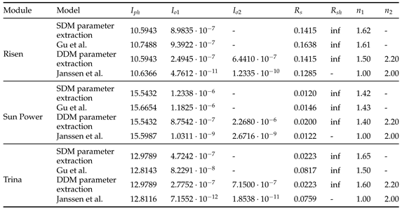
Finally, for a comparison with the parameters calculated from each employed model and the actual IV curve, direct parameter extraction is conducted using experimental data obtained from DS measurements. The obtained parameters are shown in Table 3. Since Bhang et al. model utilizes each set of parameters directly estimated, it will not be analyzed in this section.
Gu et al. and Janssen et al. use SDM and DDM respectively, each obtained parameter is compared with the corresponding model parameter estimation. Each parameter obtained from direct extraction is evaluated in the IV curve and its respective error when compared with experimental data is calculated and presented in Figure 20, Figure 21, Figure 22. It is evident that the errors for both models decreased considerably, considering that Gu et al.’s model reached percent errors above and with direct parameter extraction does not exceed . In the case of Janssen et al.’s model, using their approximations to obtain the DDM parameters they reached error higher than in the worst case, while the direct DDM extraction, as well as the SDM extraction, does not exceed .
Gu et al. and Janssen et al. used different methods, SDM and DDM respectively, to get certain parameters. Each parameter obtained was compared with what the models predicted. Then, these parameters are used to trace the modeled IV curve. Then, the percent error for modeled and experimental IV curves are calculated, shown in Figure 20, Figure 21, Figure 22. When direct extraction is applied errors decreased significantly compared to the models’ predictions, considering that Gu et al.’s model reached percent errors above and with direct parameter extraction does not exceed . In the case of Janssen et al.’s model, using their approximations to obtain the DDM parameters they reached error higher than in the worst case, while the direct DDM extraction, as well as the SDM extraction, does not exceed .
From the comparison, it seems that the principal problem associated at Janssen et al.’s model is their parameter estimation for and , since they are assumed instead of being calculated. Another difference is the value of and , with 4 magnitude orders of difference. The photocurrent also shows differences, however, they are minimal compared to the effects caused by the use of the other parameters.
On the other hand, since Gu et al.’s model is the one that presents the best performance, it will be subjected to a sensibility analysis of its parameters to identify which one has the greatest impact on its error.
Figure 23, Figure 24, Figure 25 illustrate various scenarios wherein each parameter, as derived through the method delineated by Gu, is contrasted with those acquired via SDM parameter extraction from experimental IV curve analysis. The designation “Gu” denotes parameters obtained without any alterations, while “Iph” signifies parameters obtained with the substitution of photocurrent values sourced directly from parameter extraction. Similar designations, namely “Io”, “Rs”, “Rsh”, and “n” denote scenarios wherein all parameters remain consistent with those obtained through Gu’s method, except for the specific parameter indicated in the legend, which is substituted with its SDM-extracted counterpart. Notably, the designation “Est” denotes the error observed when all parameters are derived exclusively through SDM parameter estimation.
The figures presented in Figure 23, Figure 24 highlight that the most accurate results were achieved through SDM parameter estimation using experimental IV curves. The influence of variations is most pronounced at the onset of the IV curve, which accounts for the near-zero errors observed in the “Iph” and “Est” cases. Conversely, the “Gu” and “Rsh” scenarios exhibit similar behavior, as they both utilize identical parameters due to resulting in ∞. Subsequently, the most effective substitution leading to minimized errors post SDM parameter estimation involves replacing .
The case obtained in Figure 25 behaves differently compared to the previous ones since the replacement of and n generated errors that resulted higher than for the case of n and even higher than for the case of . Those differences can be caused principally for the impact that those two parameters have in the shape of IV curve, which can be generate differences in .
6. Conclusions
The evaluation conducted with SS illumination highlights the significant impact of shadowing induced by frames or junction boxes, not only resulting in elevated errors in current but also manifesting as disparities in when comparing frontal and rear IV curves.
Among the array of models scrutinized in existing literature, the assessment focused on three proposals aimed at determining the optimal fit for IV and PV curves of bifacial PV modules: a single-diode model, a parallel single-diode model, and a double-diode model. Chosen primarily for their replicability, these models were subjected to a meticulous methodology encompassing parameter treatment advocated by each respective author, spanning both frontal and rear sides of the modules to derive the final IV curve. Our evaluation unveiled that the model proposed by Gu et al. yielded the lowest errors, approximately in the worst case. However, efforts to mitigate these errors through direct parameter extraction with SDM revealed notable disparities between estimations. Notably, the parameter with the most pronounced impact was Io, which demonstrated the potential to reduce errors if accurately calculated, as evidenced in the case of SunPower modules, where errors decreased from approximately to . Conversely, inaccurate determination of Io, as observed in the case of Trina modules, resulted in errors exceeding when directly extracted was replaced.
This research significantly contributes to the literature by offering an evaluation of existing models using data collected under controlled conditions, thereby reducing uncertainty in irradiance and temperature. Furthermore, this analysis identifies the parameters and their respective effects, shedding light on the parameter with the most substantial impact on the curve.
This study suggests two potential avenues for future research. Firstly, there is a need for the evaluation of the same models under outdoor conditions, encompassing diverse temperatures and non-uniform irradiance patterns. Such research would provide insights into model performance under real-world environmental variations. Secondly, there is an opportunity for the development of a novel approach to accurately estimate the requisite parameters, with the aim of minimizing errors in model predictions. This endeavor would contribute to advancing the accuracy and reliability of PV module modeling techniques.
Acknowledgments
The authors express their gratitude for the financial support from ANID-Fondecyt-11220697. Also, there is financial support from the Scientific Research Initiation Program (PIIC) of the Universidad Técnica Federico Santa María.
References
- Mouhib, E.; Micheli, L.; Almonacid, F.M.; Fernández, E.F. Overview of the Fundamentals and Applications of Bifacial Photovoltaic Technology: Agrivoltaics and Aquavoltaics. Energies 2022, 15. [Google Scholar] [CrossRef]
- Cuevas, A.; Luque, A.; Eguren, J.; del Alamo, J. 50 Per cent more output power from an albedo-collecting flat panel using bifacial solar cells. Solar Energy 1982, 29, 419–420. [Google Scholar] [CrossRef]
- Eisenberg, N.P.; Drori, A.; Karsenty, A.; Bordin, N.; Kreinin, L.B. Experimental Analysis of the Increases in Energy Generation of Bifacial Over Mono-Facial PV Modules. 2011.
- Tina, G.M.; Bontempo Scavo, F.; Merlo, L.; Bizzarri, F. Comparative analysis of monofacial and bifacial photovoltaic modules for floating power plants. Applied Energy 2021, 281, 116084. [Google Scholar] [CrossRef]
- Rodríguez-Gallegos, C.D.; Bieri, M.; Gandhi, O.; Singh, J.P.; Reindl, T.; Panda, S. Monofacial vs bifacial Si-based PV modules: Which one is more cost-effective? Solar Energy 2018, 176, 412–438. [Google Scholar] [CrossRef]
- Tahir, F.; Baloch, A.A.; Al-Ghamdi, S.G. Impact of climate change on solar monofacial and bifacial Photovoltaics (PV) potential in Qatar. Energy Reports 2022, 8, 518–522. [Google Scholar] [CrossRef]
- Lindsay, N.; Libois, Q.; Badosa, J.; Migan-Dubois, A.; Bourdin, V. Errors in PV power modelling due to the lack of spectral and angular details of solar irradiance inputs. Solar Energy 2020, 197, 266–278. [Google Scholar] [CrossRef]
- Antonanzas, J.; Osorio, N.; Escobar, R.; Urraca, R.; de Pison, F.M.; Antonanzas-Torres, F. Review of photovoltaic power forecasting. Solar Energy 2016, 136, 78–111. [Google Scholar] [CrossRef]
- Liang, T.S.; Pravettoni, M.; Deline, C.; Stein, J.S.; Kopecek, R.; Singh, J.P.; Luo, W.; Wang, Y.; Aberle, A.G.; Khoo, Y.S. A review of crystalline silicon bifacial photovoltaic performance characterisation and simulation. Energy Environ. Sci. 2019, 12, 116–148. [Google Scholar] [CrossRef]
- Photovoltaic devices - Part 1-2: Measurement of current-voltage characteristics of bifacial photovoltaic (PV) devices. Technical specification, International Electrotechnical Commision, 2019.
- Liang, T.S.; Poh, D.; Pravettoni, M. Challenges in the pre-normative characterization of bifacial photovoltaic modules. Energy Procedia 2018, 150, 66–73. [Google Scholar] [CrossRef]
- Razongles, G.; Sicot, L.; Joanny, M.; Gerritsen, E.; Lefillastre, P.; Schroder, S.; Lay, P. Bifacial Photovoltaic Modules: Measurement Challenges. Energy Procedia 2016, 92, 188–198. [Google Scholar] [CrossRef]
- Bhang, B.G.; Lee, W.; Kim, G.G.; Choi, J.H.; Park, S.Y.; Ahn, H.K. Power Performance of Bifacial c-Si PV Modules With Different Shading Ratios. IEEE Journal of Photovoltaics 2019, 9, 1413–1420. [Google Scholar] [CrossRef]
- Janssen, G.; Van Aken, B.; Carr, A.; Mewe, A. Outdoor Performance of Bifacial Modules by Measurements and Modelling. Energy Procedia 2015, 77, 364–373. [Google Scholar] [CrossRef]
- Ahmed, E.M.; Aly, M.; Mostafa, M.; Rezk, H.; Alnuman, H.; Alhosaini, W. An Accurate Model for Bifacial Photovoltaic Panels. Sustainability 2023, 15. [Google Scholar] [CrossRef]
- Bouchakour, S.; Valencia-Caballero, D.; Luna, A.; Roman, E.; Boudjelthia, E.A.K.; Rodríguez, P. Modelling and Simulation of Bifacial PV Production Using Monofacial Electrical Models. Energies 2021, 14. [Google Scholar] [CrossRef]
- Gu, W.; Ma, T.; Li, M.; Shen, L.; Zhang, Y. A coupled optical-electrical-thermal model of the bifacial photovoltaic module. Applied Energy 2020, 258, 114075. [Google Scholar] [CrossRef]
- Vergura, S. Simulink model of a bifacial PV module based on the manufacturer datasheet. Renewable Energy and Power Quality Journal 2020, 18, 637–641. [Google Scholar] [CrossRef]
- Lagunas, A.; Cuadra, J.; Petrina, I.; Mayo, M.E. Design of a Special Set-Up for the I-V Characterization of Bifacial Photovoltaic Solar Cells. 2008. [CrossRef]
- Zhang, Y.; Gao, Q.; Yu, Y.; Liu, Z. Comparison of Double-Side and Equivalent Single-Side Illumination Methods for Measuring the I–V Characteristics of Bifacial Photovoltaic Devices. IEEE Journal of Photovoltaics 2018, 8, 1–7. [Google Scholar] [CrossRef]
- Babu, B.C.; Gurjar, S. A Novel Simplified Two-Diode Model of Photovoltaic (PV) Module. IEEE Journal of Photovoltaics 2014, 4, 1156–1161. [Google Scholar] [CrossRef]
- Raina, G.; Sinha, S. A comprehensive assessment of electrical performance and mismatch losses in bifacial PV module under different front and rear side shading scenarios. Energy Conversion and Management 2022, 261, 115668. [Google Scholar] [CrossRef]
Figure 1.
Single diode model adapted for bifacial PV devices.
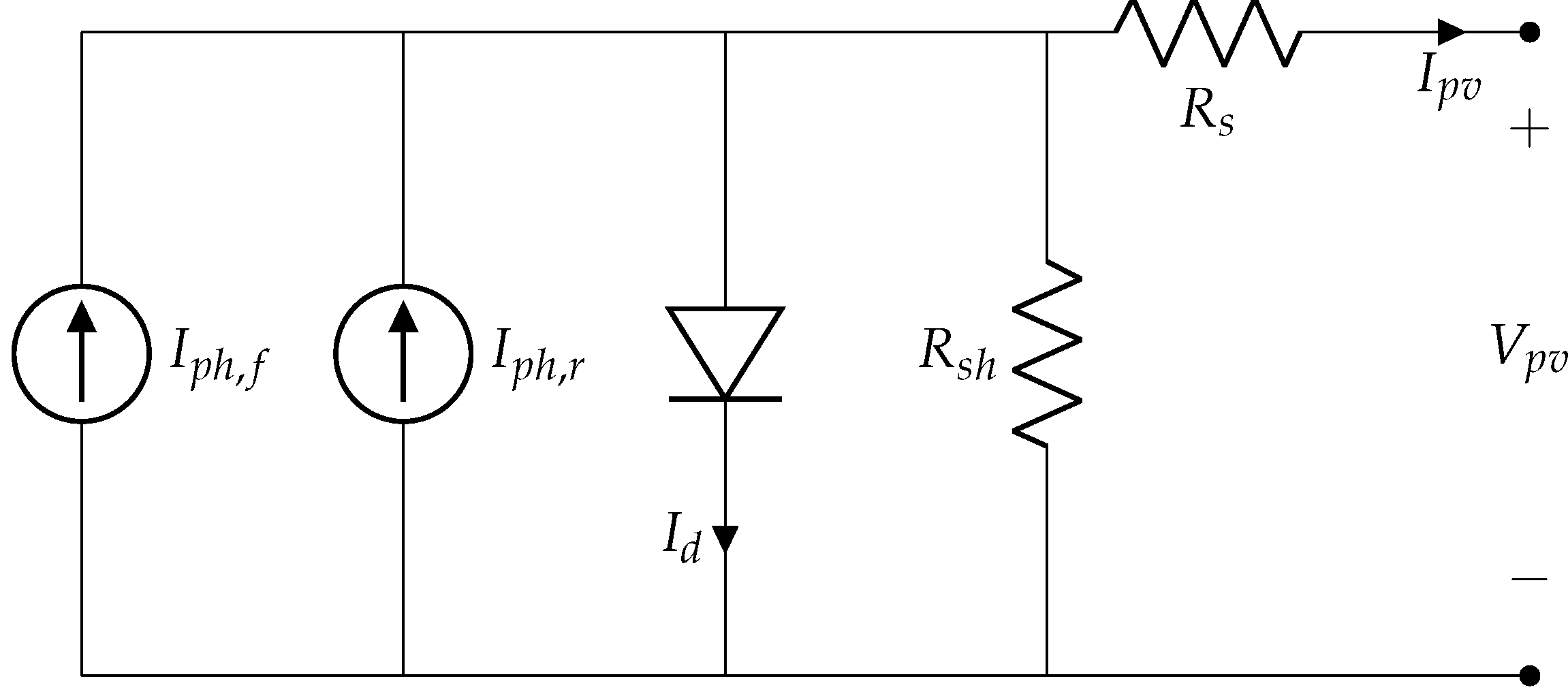
Figure 2.
Paralell configuration of the single diode model for bifacial PV devices.
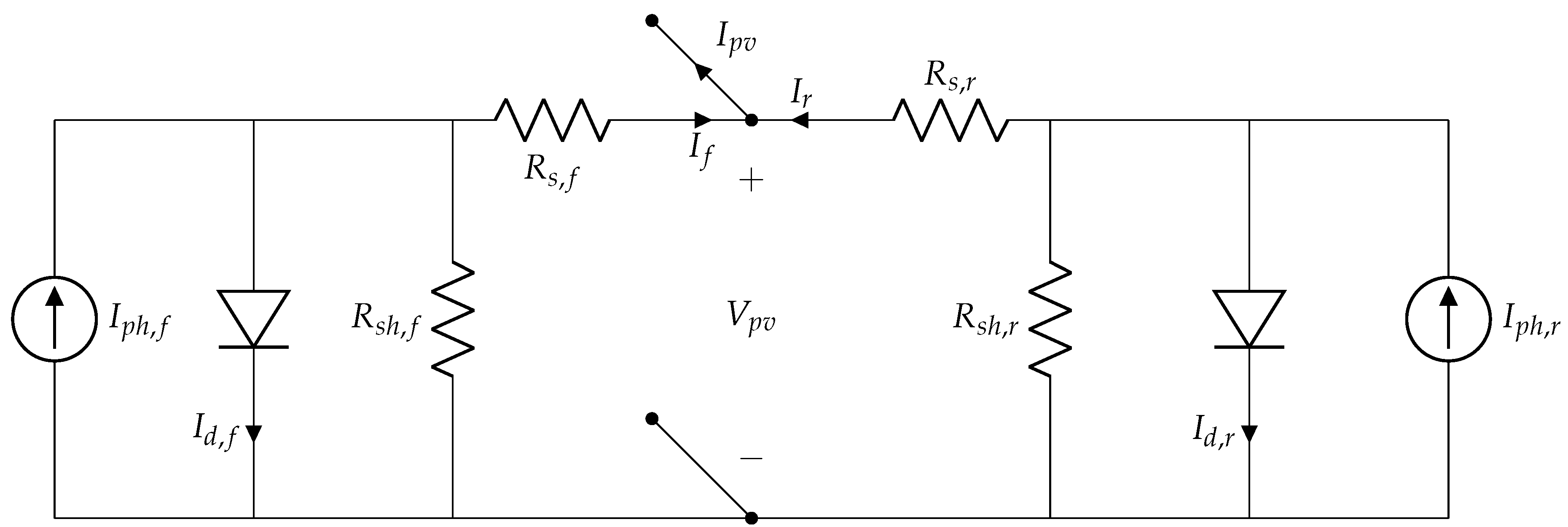
Figure 3.
Double diode model adapted for bifacial PV devices.
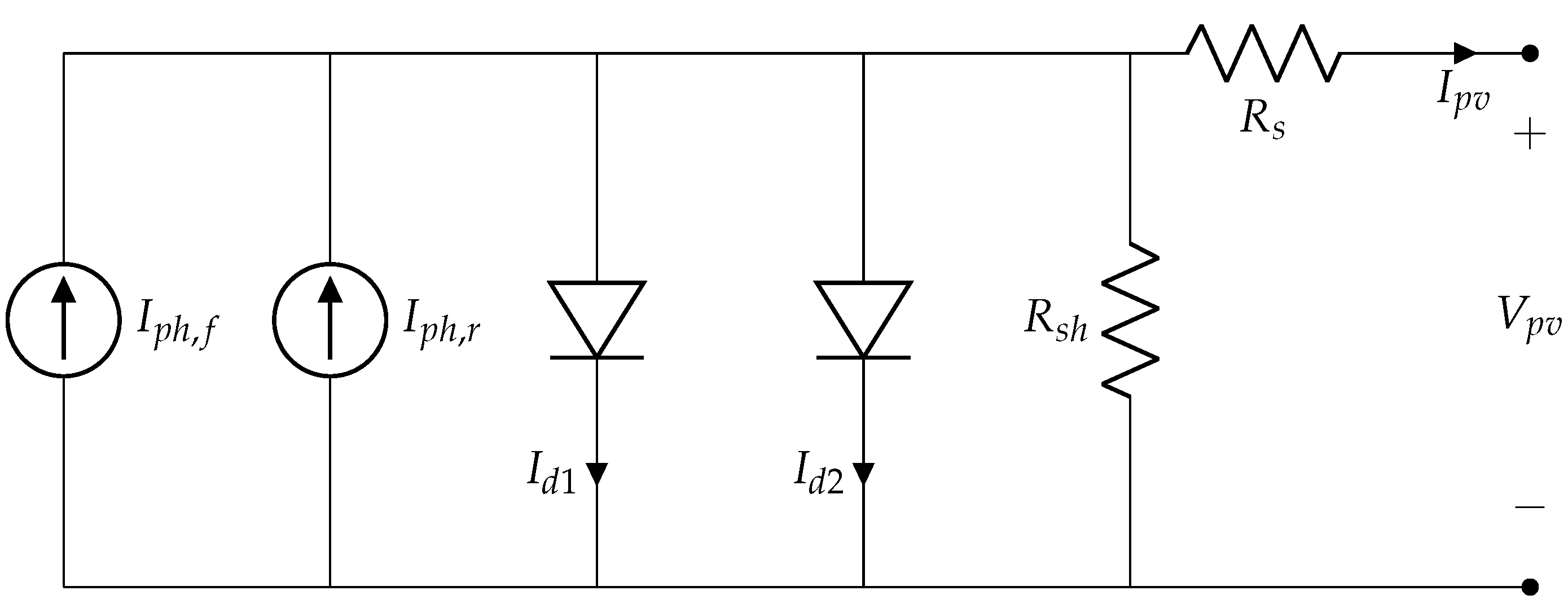
Figure 4.
Solar simulator setup for single-sided measurement.
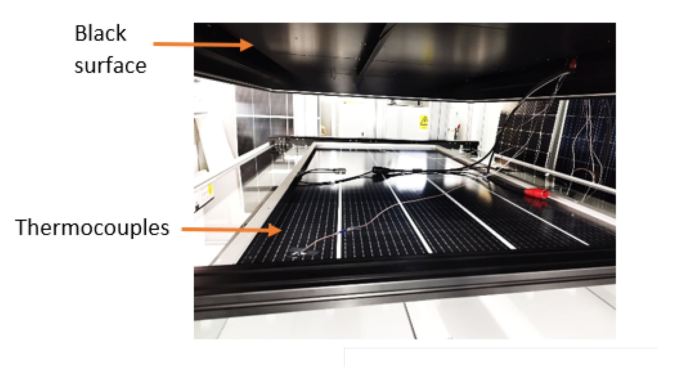
Figure 5.
Solar simulator setup for double-sided measurement.
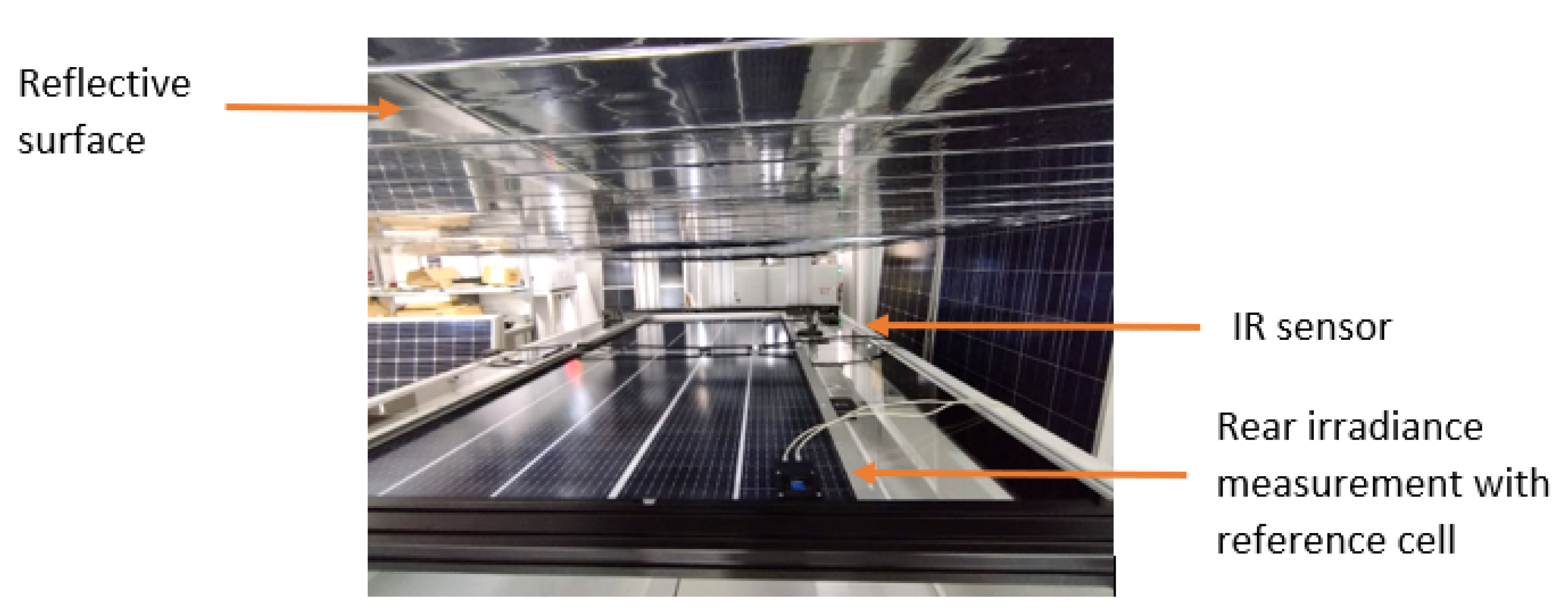
Figure 6.
Rear irradiance measuring points to evaluate uniformity in the surface of the module.
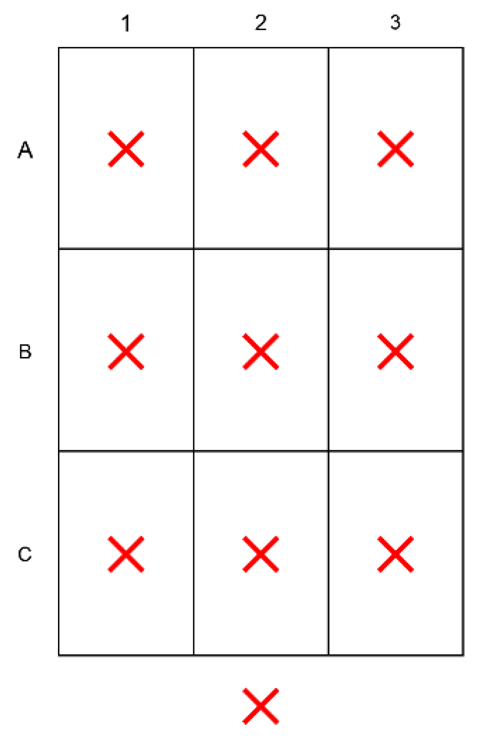
Figure 7.
Single-sided illumination measurement explanation scheme.
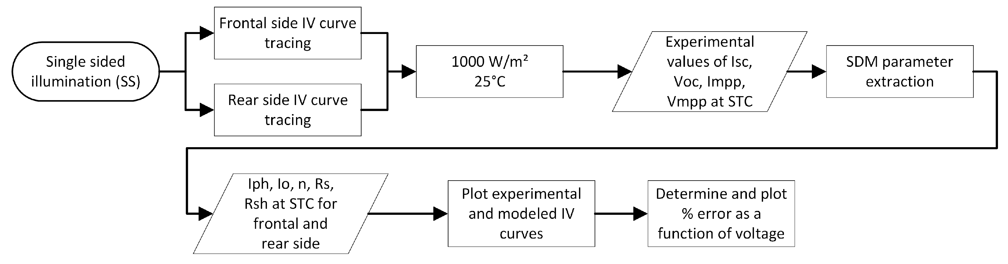
Figure 9.
(a) IV curves for frontal and rear faces of Risen RSM72-6-370BMDG and (b) current difference between experimental data and model results.
Figure 9.
(a) IV curves for frontal and rear faces of Risen RSM72-6-370BMDG and (b) current difference between experimental data and model results.
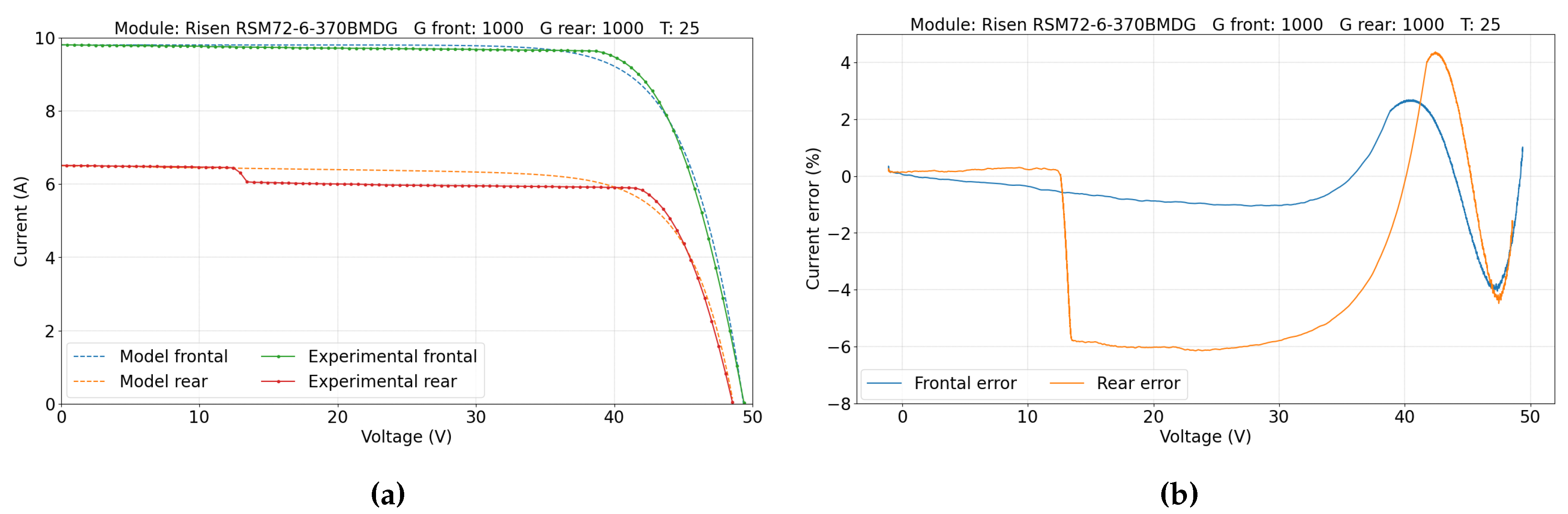
Figure 10.
(a) IV curves for frontal and rear faces of SunPower SPR-P6-500-COM-S-BF and (b) current difference between experimental data and model results.
Figure 10.
(a) IV curves for frontal and rear faces of SunPower SPR-P6-500-COM-S-BF and (b) current difference between experimental data and model results.
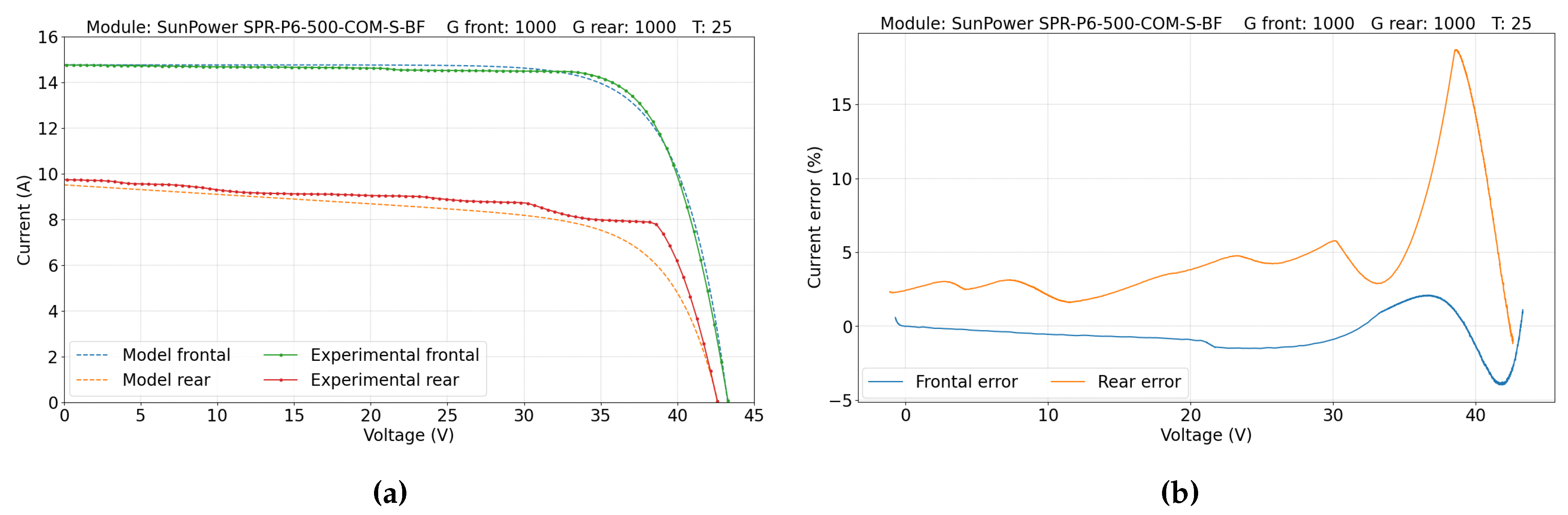
Figure 11.
(a) IV curves for frontal and rear faces of HET GO25 and (b) current difference between experimental data and model results.
Figure 11.
(a) IV curves for frontal and rear faces of HET GO25 and (b) current difference between experimental data and model results.
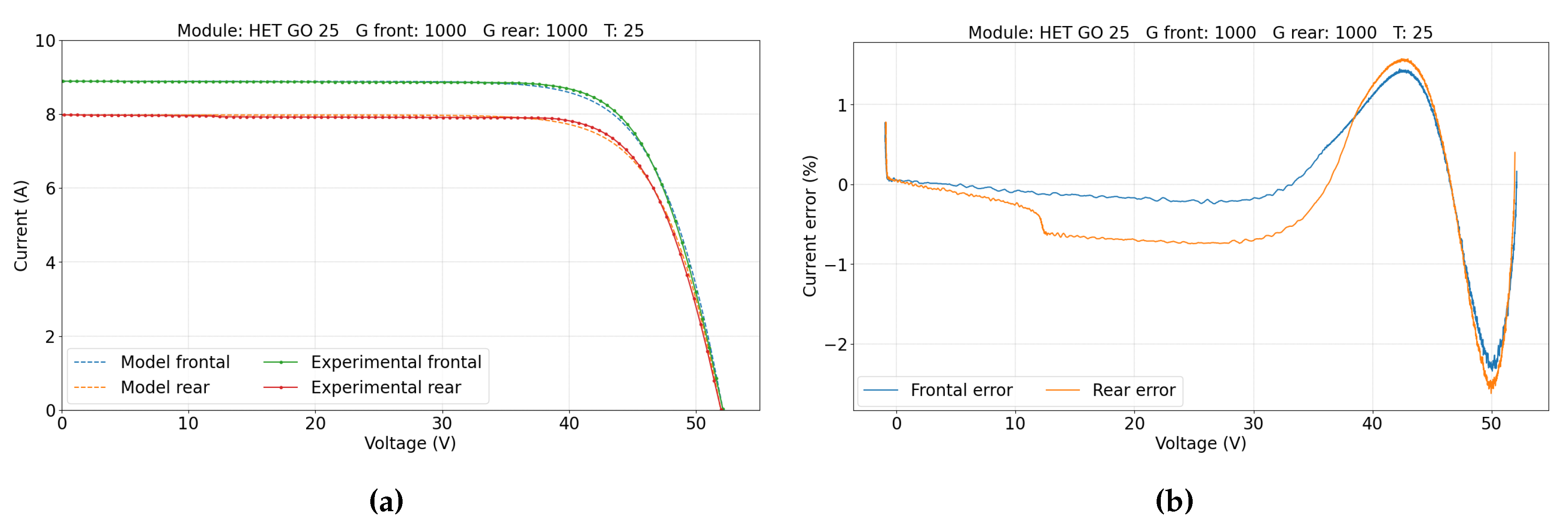
Figure 12.
(a) IV curves for frontal and rear faces of HJT GOPV PSDA 6 and (b) current difference between experimental data and model results.
Figure 12.
(a) IV curves for frontal and rear faces of HJT GOPV PSDA 6 and (b) current difference between experimental data and model results.
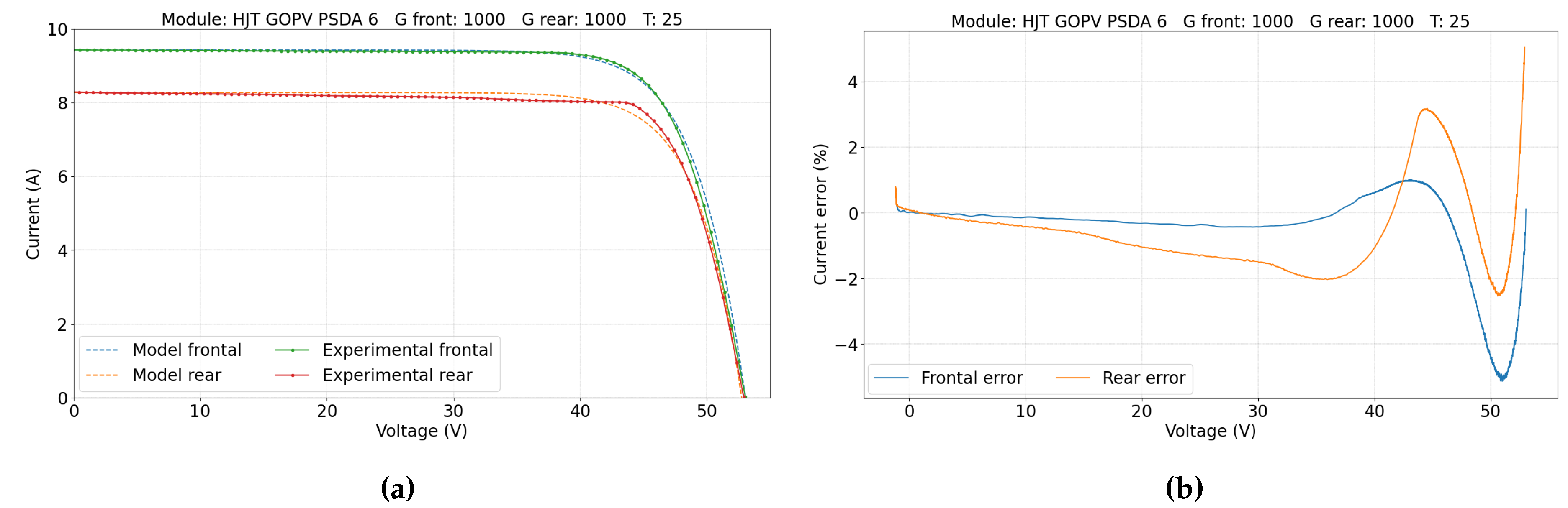
Figure 13.
(a) IV curves for frontal and rear faces of n-PERT and (b) current difference between experimental data and model results.
Figure 13.
(a) IV curves for frontal and rear faces of n-PERT and (b) current difference between experimental data and model results.
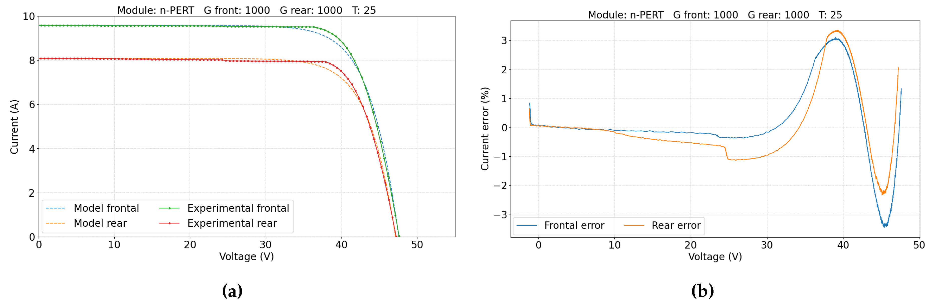
Figure 14.
(a) IV and PV curves for experimental and modeled data, an (b) current and power differences between each model and experimental data, illustrated for module Risen RSM72-6-370BMDG.
Figure 14.
(a) IV and PV curves for experimental and modeled data, an (b) current and power differences between each model and experimental data, illustrated for module Risen RSM72-6-370BMDG.
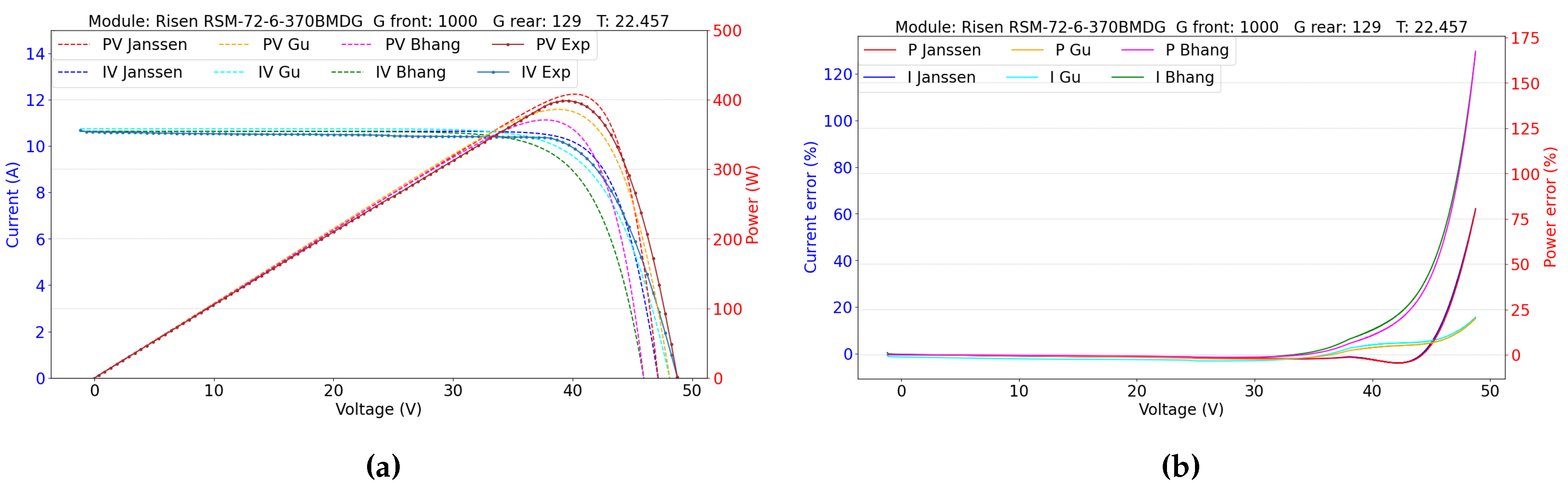
Figure 15.
(a) IV and PV curves for experimental and modeled data, an (b) current and power differences between each model and experimental data, illustrated for module SunPower SPR-P6-500-COM-S-BF.
Figure 15.
(a) IV and PV curves for experimental and modeled data, an (b) current and power differences between each model and experimental data, illustrated for module SunPower SPR-P6-500-COM-S-BF.
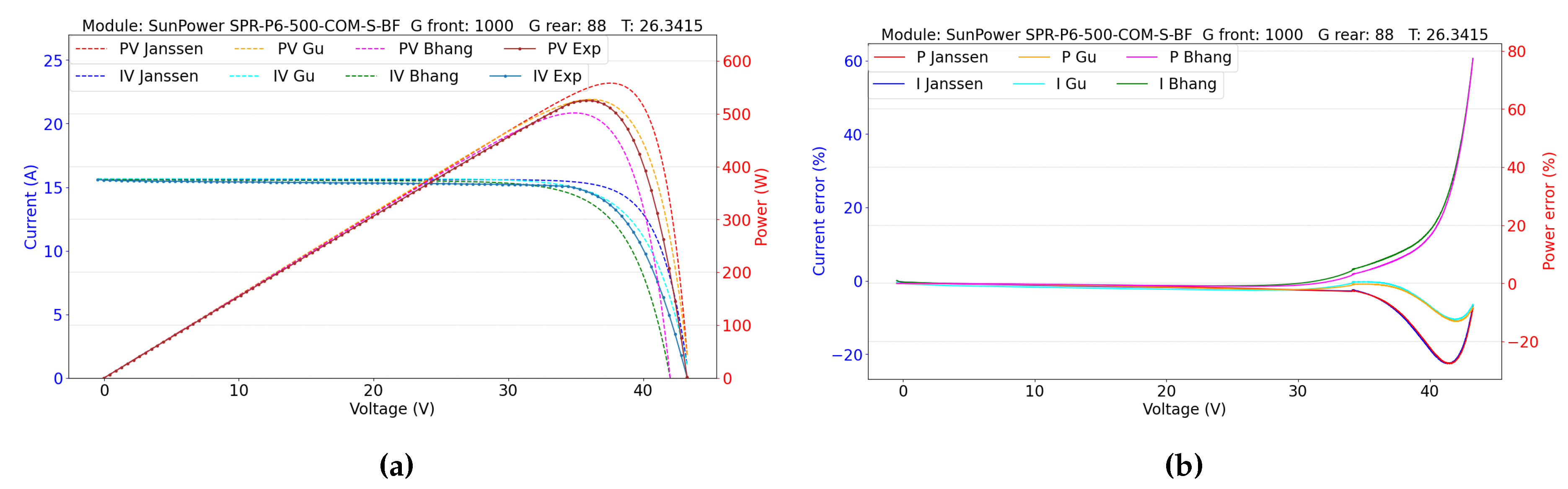
Figure 16.
(a) IV and PV curves for experimental and modeled data, an (b) current and power differences between each model and experimental data, illustrated for module Trina TSM-DE18M(II).
Figure 16.
(a) IV and PV curves for experimental and modeled data, an (b) current and power differences between each model and experimental data, illustrated for module Trina TSM-DE18M(II).
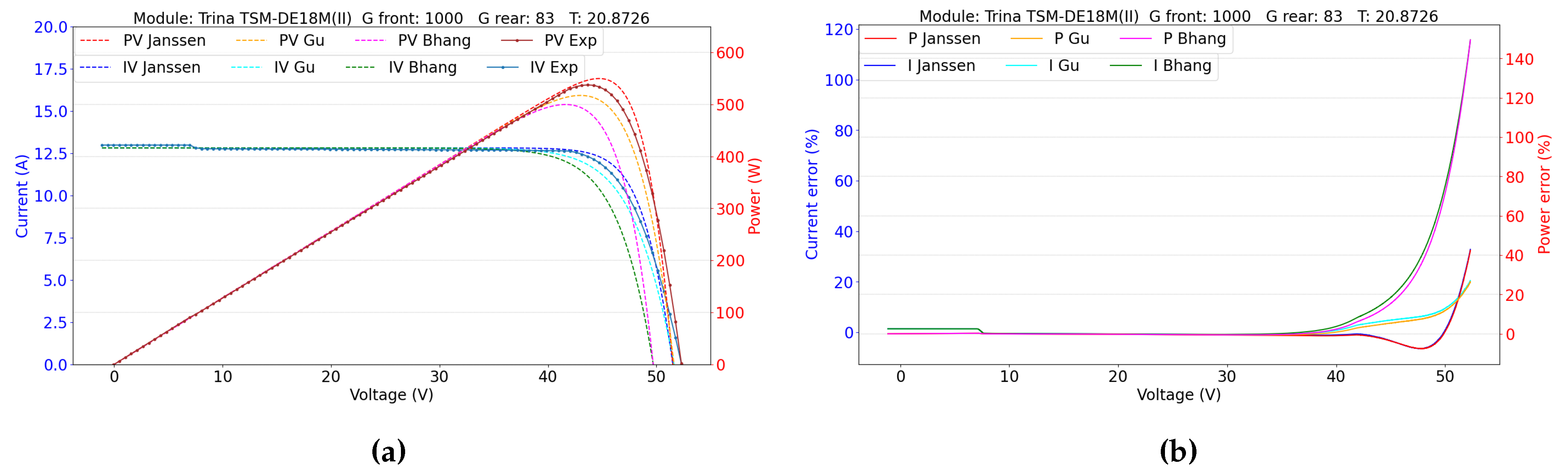
Figure 17.
Difference between (a) Pmax and (b) current at the last data series point for experimental and modeled data for the Risen RSM-72-6-370BMDG module.
Figure 17.
Difference between (a) Pmax and (b) current at the last data series point for experimental and modeled data for the Risen RSM-72-6-370BMDG module.
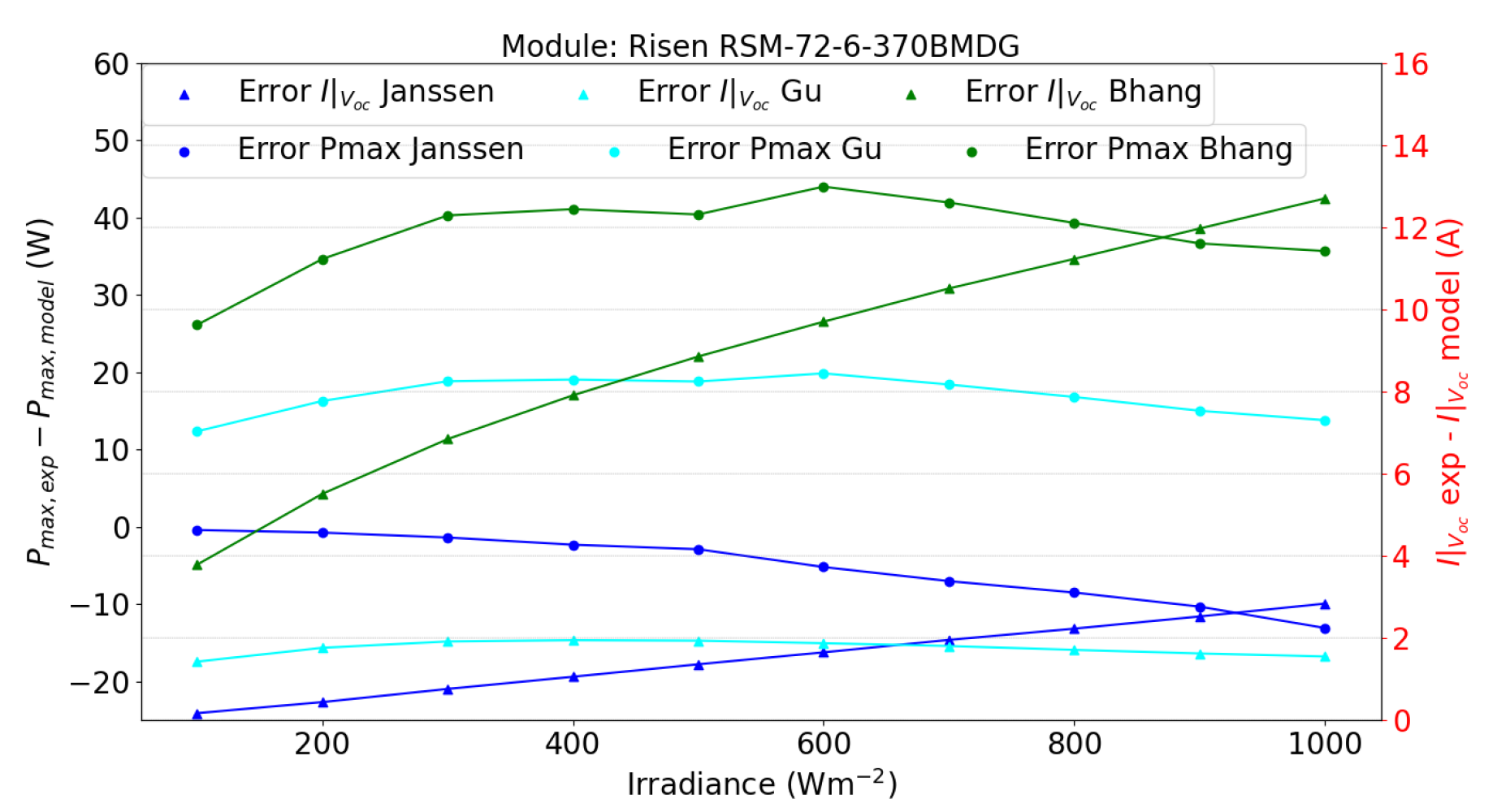
Figure 18.
Difference between (a) Pmax and (b) current at the last data series point for experimental and modeled data for the SunPower SPR-P6-500-COM-S-BF module.
Figure 18.
Difference between (a) Pmax and (b) current at the last data series point for experimental and modeled data for the SunPower SPR-P6-500-COM-S-BF module.
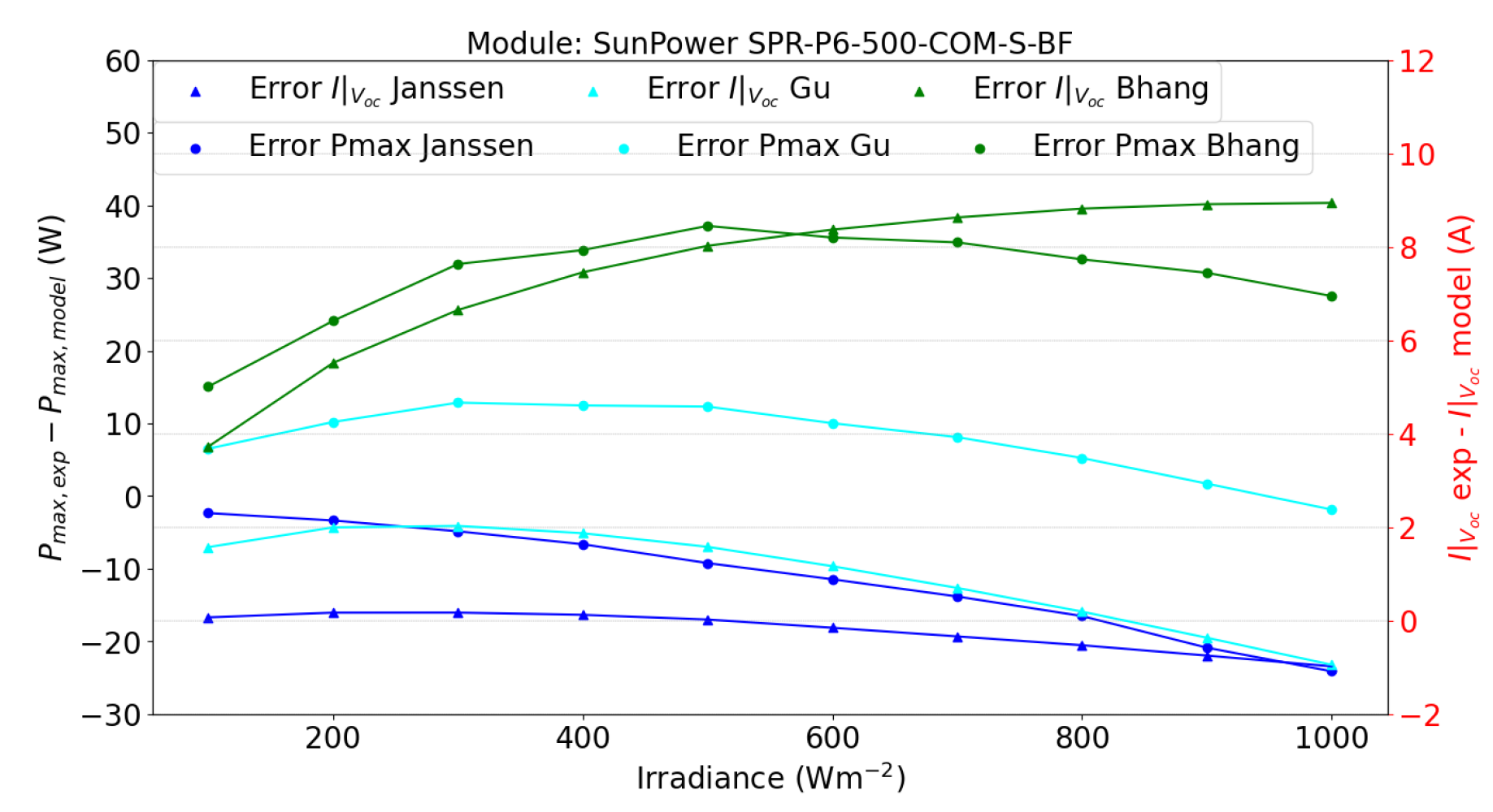
Figure 19.
Difference between (a) Pmax and (b) current at the last data series point for experimental and modeled data for the Trina TSM-DE 18M(II) module.
Figure 19.
Difference between (a) Pmax and (b) current at the last data series point for experimental and modeled data for the Trina TSM-DE 18M(II) module.
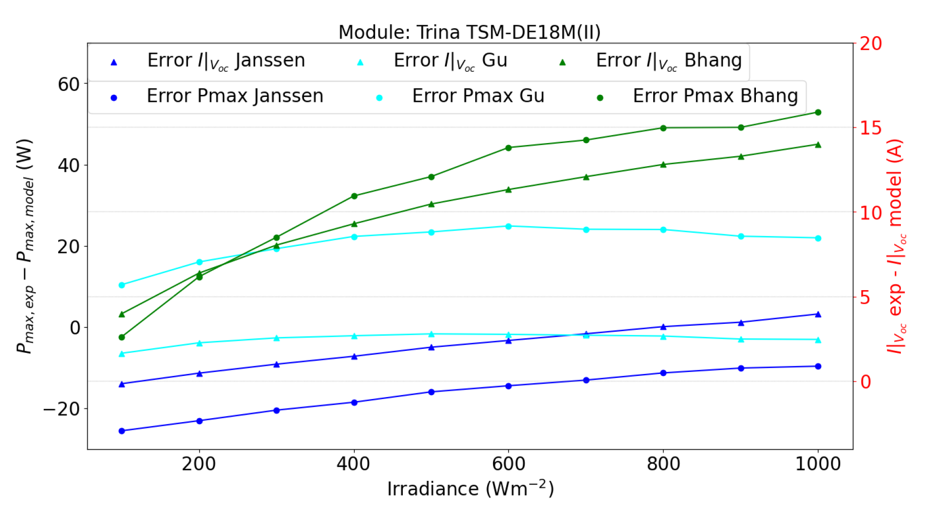
Figure 20.
IV and PV curves percent error for direct parameter extraction for (a) SDM (b) DDM for module Risen RSM72-6-370BMDG, considering parameters showed in Table 3.
Figure 20.
IV and PV curves percent error for direct parameter extraction for (a) SDM (b) DDM for module Risen RSM72-6-370BMDG, considering parameters showed in Table 3.
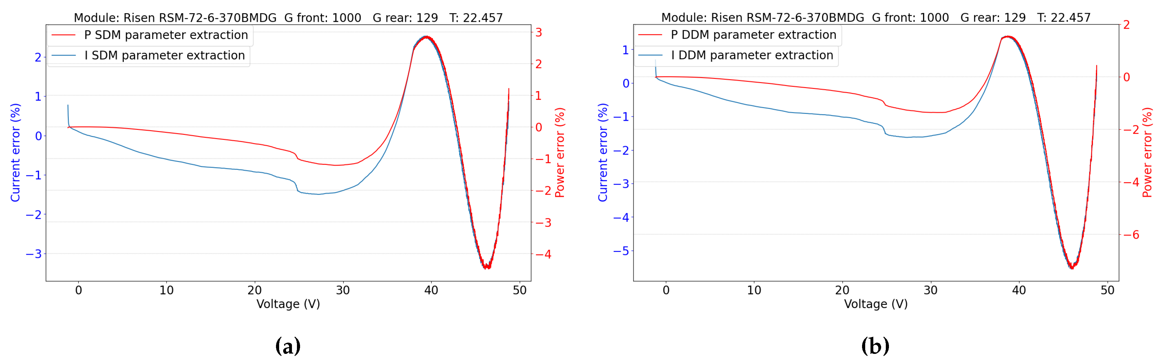
Figure 21.
IV and PV curves percent error for direct parameter extraction for (a) SDM (b) DDM for module SunPower SPR-P6-500-COM-S-BF, considering parameters showed in Table 3.
Figure 21.
IV and PV curves percent error for direct parameter extraction for (a) SDM (b) DDM for module SunPower SPR-P6-500-COM-S-BF, considering parameters showed in Table 3.
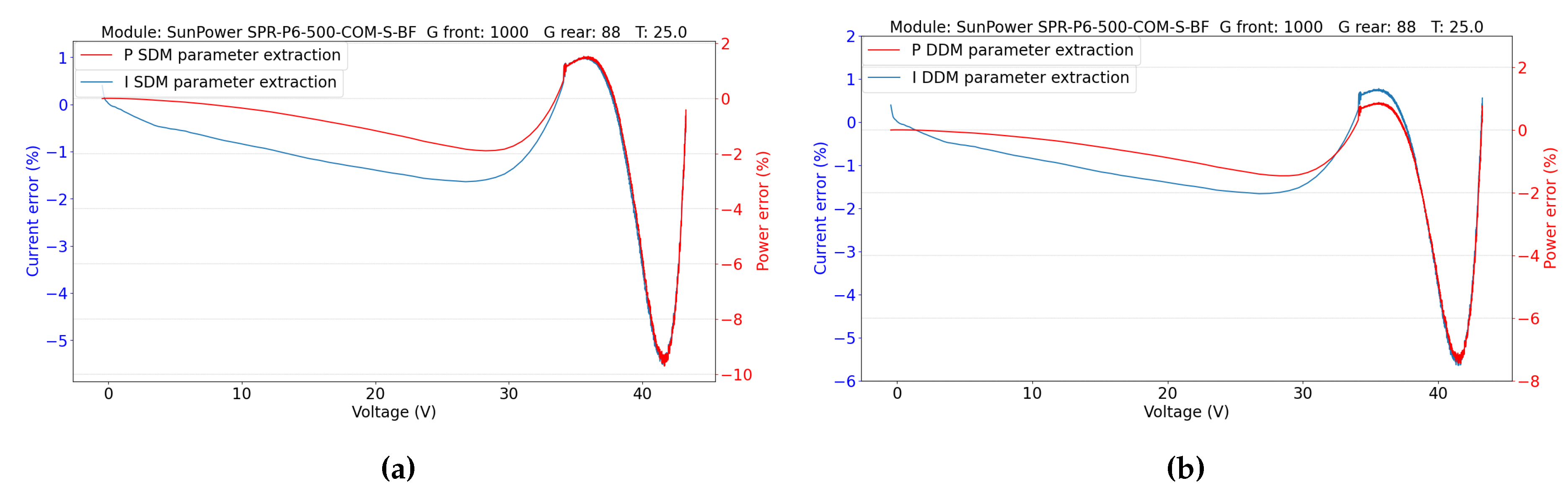
Figure 22.
IV and PV curves percent error for direct parameter extraction for (a) SDM (b) DDM for module Trina TSM-DE18M(II), considering parameters showed in Table 3.
Figure 22.
IV and PV curves percent error for direct parameter extraction for (a) SDM (b) DDM for module Trina TSM-DE18M(II), considering parameters showed in Table 3.
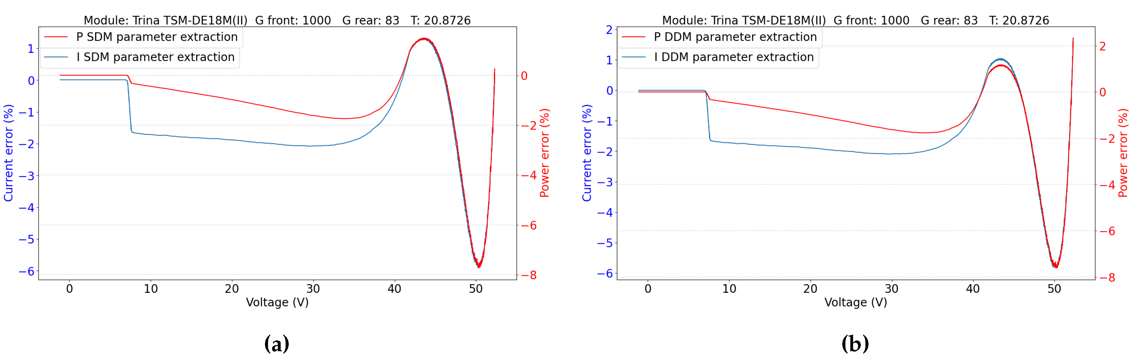
Figure 23.
Current error when obtained parameters are changed for the estimated SDM parameters for module Risen RSM-72-6-370BMDG.
Figure 23.
Current error when obtained parameters are changed for the estimated SDM parameters for module Risen RSM-72-6-370BMDG.
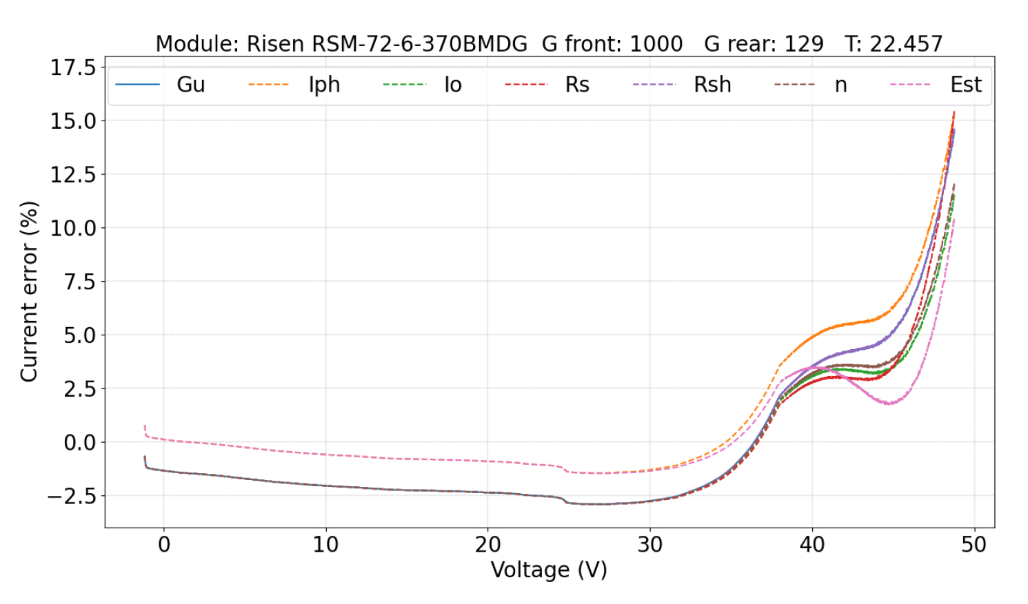
Figure 24.
Current error when obtained parameters are changed for the estimated SDM parameters for module SunPower SPR-P6-500-COM-S-BF.
Figure 24.
Current error when obtained parameters are changed for the estimated SDM parameters for module SunPower SPR-P6-500-COM-S-BF.
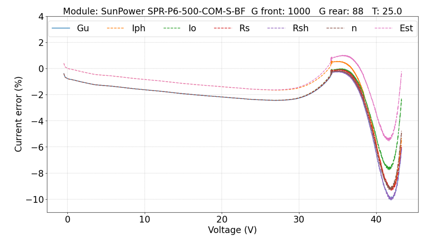
Figure 25.
Current error when obtained parameters are changed for the estimated SDM parameters for module Trina TSM-DE18M(II).
Figure 25.
Current error when obtained parameters are changed for the estimated SDM parameters for module Trina TSM-DE18M(II).
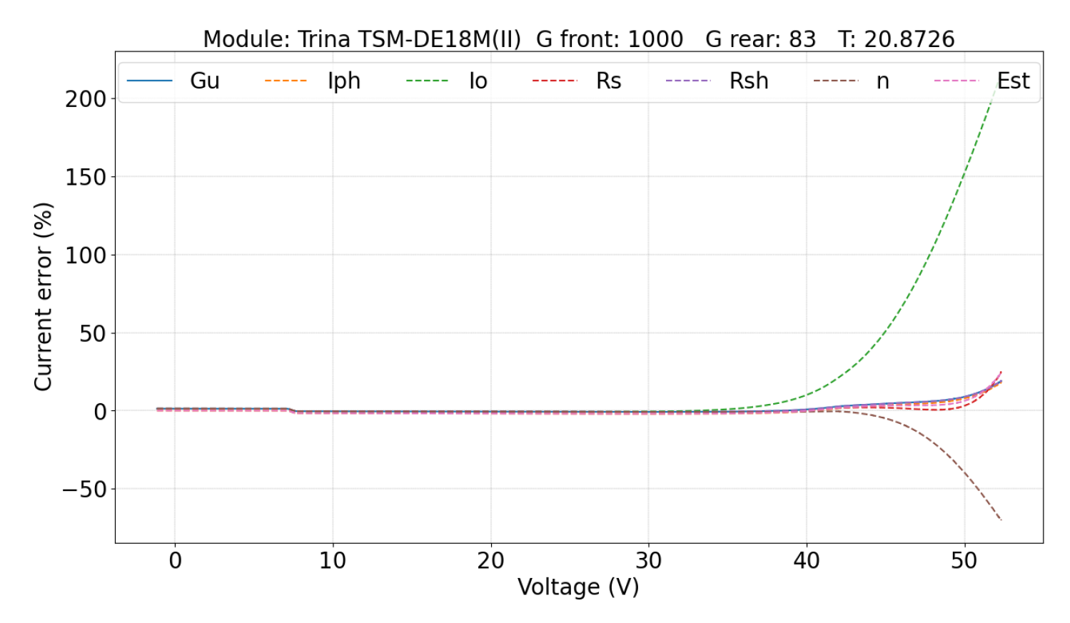
Table 2.
Modules utilized for IV curve tracing with the sun simulator.
| Module | Pmax (W) | Technology | Test |
|---|---|---|---|
| Risen RSM72-6-370BMDG | 370 | PERC+ | SS, DS |
| GOPV PSDA 6 | 393 | HJT | SS |
| HET GO 25 | 355 | HJT | SS |
| n-PERT | 348 | n-PERT | SS |
| Trina TSM-490DEG18MC.20(II) | 490 | PERC+ | DS |
| SunPower SPR-P6-500-COM-S-BF | 500 | PERC+ | SS, DS |
Table 3.
Parameters obtained from every bifacial model employed and compared with direct extraction using SDM and DDM.
Table 3.
Parameters obtained from every bifacial model employed and compared with direct extraction using SDM and DDM.
 |
Disclaimer/Publisher’s Note: The statements, opinions and data contained in all publications are solely those of the individual author(s) and contributor(s) and not of MDPI and/or the editor(s). MDPI and/or the editor(s) disclaim responsibility for any injury to people or property resulting from any ideas, methods, instructions or products referred to in the content. |
© 2024 by the authors. Licensee MDPI, Basel, Switzerland. This article is an open access article distributed under the terms and conditions of the Creative Commons Attribution (CC BY) license (http://creativecommons.org/licenses/by/4.0/).
Copyright: This open access article is published under a Creative Commons CC BY 4.0 license, which permit the free download, distribution, and reuse, provided that the author and preprint are cited in any reuse.


