Submitted:
18 November 2024
Posted:
19 November 2024
You are already at the latest version
Abstract
Transformers are essential machines in electrical energy distribution systems, which is why more efficient technologies for power transformers have been developed for decades. This has not been the case for mall transformers used in low voltage circuits, in literature there is little knowledge about his efficiency. This work seek to determine the efficiency of conventional transformers used in low voltage through a methodology that includes an analytical method and experimental tests. Three transformers in the Dominican Republic market are selected, two of 900 VA and one of 1500 VA, all step-downs of approximately 120 V/25 V. The initial load is a resistive load of 18.4 Ω. The results indicate that the efficiencies are in the range of 47 to 86.5%, considering variations in the load. The highest efficiency of the transformers was in the demand range of 12 to 24% of the nominal demand. In general, losses in the excitation branch in the core represent at least 90% of the losses, while losses in the windings represent the remaining part. Based on the results, a more exhaustive evaluation of the efficiency of small transformers is suggested, as well as economically evaluating the replacement of transformers with more efficient ones.
Keywords:
small autotransformers
; efficiency
; energy demand
; low voltage installations
1. Introduction
Since the type of current used for the transmission of electric power from generating plants to consumption points is based on alternating current, electrical transformers are indispensable devices in electric power distribution systems. Any improvement in the efficiency or efficient use of these devices can result in great economic savings, considering that they can last for decades in operation [1].
For transmission and distribution systems, electronic power transformers have been developed in the last decade, which provide greater efficiency than conventional transformers [2]. Losses in distribution transformers directly harm distribution and transmission companies, which has motivated interest in reducing losses in medium and high voltage transformers [3]. The efficiency of distribution transformers currently in use is commonly above 96%.
The search for greater efficiency has also been seen in other applications, such as railway vehicles, achieving 4.7% greater efficiency and reducing its size by 7% compared to a conventional transformer. [4].
At a low voltage distribution scale, there has also been interest in determining the associated losses in residential condominiums and low voltage circuits. However, there are few studies on the efficiency of small transformers in low voltage applications (power <10 kVA). A very common case of the use of small conventional transformers (without power electronics) is in DC to AC inverters, in energy backup applications with battery storage [5] in developing countries, commonly. In this application, transformers represent a permanent load to consider, so knowing their efficiency would help to estimate the losses involved in the use of these devices, which would motivate the search for innovations that make their use more efficient. In addition, knowing the parameters of the transformers can help to determine the efficiency analytically. El-Dabah & Agwa et al [6] conducted a study to determine the electrical parameters of transformers, which is important in transformer design and efficiency prediction.
This paper aims to determine the electrical parameters of equivalent circuits of small transformers, as well as their efficiency based on these parameters. The lack of information in the literature on small low voltage transformers hides potential savings at residential and commercial levels, both for customers and for distribution companies.
The specific objectives of the research are:
1. To determine the parameters of conventional small transformers: magnetizing resistance, magnetizing reactance, equivalent series resistance and equivalent series reactance.
2. To apply a methodology to determine and study the efficiency of conventional small transformers.
The work is distributed as follows. In unit 2, the procedure to determine the parameters of electrical transformers is presented, as well as structural details of said devices, the equations used and the research methodology. In unit 3, the open circuit and short circuit test are performed, with which the parameters of the equivalent circuits are calculated; the efficiency of the transformers is determined from said parameters and also by means of an experimental method; the efficiency curve vs. the variation of a resistive load is estimated. In unit 4, the results are discussed, and in unit 5, the main conclusions are presented and recommendations are provided for an extension of the subject.
2. Materials and Methods
2.1. Operating principle
The electrical transformer is a passive component that transforms alternating voltage and current levels from one level to another. This device works according to Faraday's law, which states that the voltage induced in a coil of conducting wire is proportional to the rate of change of the magnetic flux through it [7], [8], as shown in Equation (1).
A typical diagram of a transformer is shown in Figure 1. In a transformer, the variable magnetic flux is produced by applying a sinusoidal voltage of effective value to the primary winding, which has turns. By means of the transformer core, the flux passes through the secondary winding of turns and a sinusoidal voltage of effective value is induced. Since the flux passes almost entirely from one winding to the other by means of the core, by applying Equation (2) to both windings, Equation (2) is obtained, which is known as the transformation ratio.
The number of turns per volt of applied alternating current corresponds to the frequency of the sinusoidal voltage and the amplitude of the saturation magnetic flux density of the transformer core. [9].
2.2. Approximate equivalent circuit and parameters of a transformer
A transformer can be modeled by means of approximate circuits that facilitate its analysis. Figure 2 shows two approximate equivalent circuits of a transformer. Figure 2A shows the circuit referred to the primary and Figure 2B shows the circuit referred to the secondary. For more details on equivalent transformer circuits, it is recommended to consult Chapter 2 of Chapman [10]. In Figure 2 (B), the equivalent series resistance referred to the secondary is determined by Req S =ReqP/a2 and the equivalent series reactance referred to the secondary by Xeq S = XeqP /a2.
As is known in the literature, the parameters of the transformer model in Figure 2 can be approximated by two tests: the open circuit test and the short circuit test.
In the open circuit test, the magnetizing resistance of the core and the magnetizing reactance are determined. To do this, the primary winding of the transformer is connected to the nominal voltage and the secondary winding is left open, as shown in Figure 3. In this test, a voltmeter is connected to measure the applied voltage, an ammeter to measure the current in the primary and a wattmeter to measure the potential in the primary.
From this information the power factor of the input current is determined and hence the magnitude and angle of the excitation impedance. The magnitude of the excitation admittance referred to the primary can be determined by means of the open circuit current () and the open circuit voltage () as shown in Equation (3). The open circuit power factor can be determined by means of Equation (4) and consequently the open circuit angle () is determined by Equation (5). Since the current lags the voltage in a real transformer, the excitation admittance is determined by Equation (6).
and are obtained by stating from Eq.uation (6), that the resistance is the reciprocal of the conductance and that the reactance is the reciprocal of the susceptance, obtaining equations (7) and (8).
In the short-circuit test, the equivalent series resistance and the equivalent series reactance ) are determined. In this test, a short circuit is made in the secondary winding and the terminals in the primary winding are connected to a voltage source much lower than the nominal voltage. The voltage in the primary is adjusted until the current flowing in the short-circuited windings is equal to its nominal value, taking care not to burn the transformer windings. The connection diagram for this test is shown in Figure 4.
The magnitude of the series impedance (referred to the primary side) is determined with Equation (9), the PF with Equation (10) and the corresponding angle () with Equation (11).
Since the magnitude of and the angle between the voltage and the current are known, can be determined by Equation (12), in turn from this equation equations (13) and (14) are obtained, which allow determining the sought parameters.
2.2. Efficiency by transformer parameters
This method seeks to evaluate the efficiency of a transformer by knowing the load, which requires an analytical procedure. In this work, a resistive load is considered, so the current in the secondary of the transformer is determined by Equation (15), where the total resistance is the sum of the resistance of the secondary winding () of the transformer and the load resistance ().
The power loss in copper () is determined from Equation (16), which depends on which is determined with Equation (15) and which is an already mentioned parameter of the transformer.
is the copper loss power determined by Equation (16) and the core power loss () is determined by Equation (17). In Equation (17), represents the magnitude of the primary voltage referred to the secondary , whose phasor expression is shown in Equation (18). This equation is obtained by applying the Kirchhoff voltage ratio in the approximate circuit model of a transformer, shown in Figure 2B; is taken as a reference for the phasor analysis. The magnitude of the phasor is obtained with Equation (19), provided that and are in phase with PF =1, which is fulfilled for a resistive load.
By definition, efficiency is the ratio between output power and input power. In the case of an electrical transformer, the efficiency in % can be determined by means of Equation (21).
To make η dependent on in each term, from Equation (19) is substituted into Equation (17),
Substituting this expression for as well as that for from Equation (17) into Equattion (20), we obtain Equation (21), which is the expression required to relate the efficiency to the current in the secondary.
2.3. Efficiency through measurement of input and output power
In this case, the transformer input power is measured, as well as the output power, then Equation (22) is used. In this case, there is only one wattmeter, so an ammeter and a voltmeter will be connected to the secondary. In order to determine the active power in the secondary, a resistive load is connected, such that PF=1.
2.4. Caso de estudio, selección de las muestras y desarrollo experimental
The case study is carried out in the Dominican Republic, a country in energy development where small transformers are used in residential applications, mainly in electrical inverters for energy backup during power outages. They are also used in electrical control circuits in the commercial and industrial sector.
In the selection criteria for small transformers, it was considered appropriate to choose transformers with low quality control and also with a more professional finish. With this, the implications of poor manufacturing practices and the reduction in efficiency would be considered. Three transformers were selected, one confessed by students from the Instituto Politécnico Loya (IPL) (called T1), one from a university project (T2) and another extracted from an inverter (called T3). Figure 5 shows the three transformers with their names. Table 1 shows the characteristics of each of the transformers for the case study. In Table 1, dP is the approximate diameter of the primary conductor and dS is the diameter of the secondary conductor; the conductor sizes [11] and their ampacity are indicated in correspondence with the diameter measured with a caliper (approximate measurement due to the inconvenience of taking the measurement). Also in Table 1: A is the cross-sectional area of the core, S is the nominal power according to the area A, Bm is the saturation magnetic flux density commonly used to determine the number of turns per volt applied to the transformer, Vp is the voltage applied to the primary of the transformer, a is the transformation ratio (Vp/VS).
Figure 6 shows the instruments used in the tests. Figure 6A shows a variable autotransformer to adjust the voltage applied to the primary, both for the open circuit test and for the short circuit test. Figure 6B shows a wattmeter [12] to measure the active power, this model also measures the current, the effective voltage and the power factor, only that it measures from 42 V, which is its minimum operating voltage. Although this model of wattmeter measures the power factor, this will be calculated with Equation (10) in order to obtain more significant figures. Figure 6C shows a clamp ammeter and a multimeter used as a voltmeter, the first one was used to measure the short circuit current in the secondary and the second one to measure the voltage applied to the primary during the short circuit test and to the secondary during the efficiency test.
For the efficiency test, a toaster as shown in Figure 6D will be used as a load, which constitutes a resistive load. The fact that it is a resistive load makes the calculation easier, since the PF is 1, and the effective power is simply the product of the measured voltage by the measured current.
2.5. Obtaining the efficiency curve vs. the load coefficient
Since the efficiency of transformers varies with the load, it is necessary to determine it for different loads. The variation of the efficiency of transformers with other loads is done by a prediction or estimation, which consists of theoretically varying the load resistance, calculating the secondary current with Equation (15) and then the results of these quantities are substituted in Equation (21) to determine the efficiency. The resistance is varied from its real value to zero, thus evaluating the efficiency up to a load close to the nominal power of the transformer (). The demanded power is calculated by Equation (23) and the percentage load coefficient (α) by Equation (24). In Equation (24), is the demanded power for .
2.6. Research Methodology
The methodology of this research is summarized in the flow chart in Figure 7. First, transformers are selected based on different applications and constructions. Then, open circuit and short circuit tests are performed for each transformer. With the data obtained, the parallel parameters of the excitation branch (RC y XM) and the series parameters (Req S y Xeq S) are calculated. Once the parameters are determined, the transformers are connected to a resistive load, the required parameters are measured and Equation (23) as well as Equation (21) are used for verification purposes between the estimated and actual efficiency. Then, from Equation (21) the efficiency curves are obtained for different values of the load resistance and the results are discussed. Finally, conclusions and recommendations are presented.
3. Resultados
3.1. Open circuit and short circuit test
Table 2 shows the data measured by the two tests. Figure 8 shows, as an illustration, the images of the actual connections for the two tests on T1. Figure 8B) shows an rms voltage of 30.6 V applied to the primary, which is not sufficient for the wattmeter to operate. It is when the applied voltage reaches 42 V that the wattmeter can measure, as shown in Figure 8C). Figure 9 and Figure 10 show the images for the connections of the two tests, for transformers T2 and T3 respectively.
Table 3 shows the values of the parameters calculated with equations 7, 8, 13 and 1
3.2. Determining efficiency from parameters and a resistive load
For the following calculations, a resistive load of 18.4 Ω was used on the secondary, however each secondary winding has its own resistance, which increases the resistance in the circuit. In this situation, the total series resistance is determined for each case.
Calculations for transformer T1
Calculations for transformer T2
Calculations for transformer T3
In the case of T3, there was a problem with the short-circuit test; T3 exceeded the power of the Variac and the current became very large, 10 A in the primary and 50 A in the secondary. However, this does not prevent estimating the parameters in the excitation branch. In addition, it has been seen that the power losses in the copper have been less than 10% of the power losses in the core in the other transformers. In this case, it is assumed that , so and are not considered.
Figure 6 Approximate circuit model referring to the secondary for transformer T1. Source: own elaboration.
3.3. Determining efficiency from input and output power
In this case, the circuit is built, the diagram of which is shown in Figure 11. The input power is measured with a wattmeter, and the voltage and current are measured with a voltmeter and ammeter on the secondary to calculate the output power. Table 4 shows the input and output powers for each transformer, as well as the results of the efficiencies for each transformer. Figure 12 shows the images of the connections for each transformer.
Estimation of efficiency curves with increasing load
Since transformer efficiency is low with small demands, it is necessary to study the efficiency behavior for various demands. To do this, the load is increased by theoretically reducing the load resistance in Equation (17) until a current is produced that demands the nominal power.
Table 5 shows 20 RL values for the case of T1, from its real value to a value of 0, since the nominal power of 900 VA was not reached, power calculated according to the area of the core. It should be noted that the caliber of the secondary winding of this transformer is much smaller than it would be if the power for which the core gives were demanded, consequently the electrical resistance of the secondary winding (0.8 Ω) prevents the maximum power that the core of T1 can provide from being reached.
For T2, Table 6 shows that if the rated power was reached with RL = 0.24 Ω, in this case the resistance of the secondary winding is 0.5 Ω. For neither of these two transformers, the secondary winding is calibrated for the rated power. The appropriate gauge for both transformers in the secondary is AWG #6, and the maximum current demanded in the secondary is 900 VA/25V= 36 A.
Table 7 shows the efficiency of T3. This case is different from that of transformers T1 and T2, because the variable voltage source did not have enough power for the demand of T3 in the short-circuit test. In addition, the wattmeter used in the tests works at a minimum rms voltage of 42 V, but already at 15 A the current in the secondary reached the maximum demand. Due to these limitations, the equivalent series resistance referred to the secondary cannot be determined. As an alternative, it was decided to give values of 0, 0.1, 0.2 and 0.3 Ω to ReqS, and thus be able to interpret the efficiency behavior, despite the limitations. From Equation (17) it was determined that the value of the equivalent series reactance referred to the secondary does not influence significantly as ReqS does, so its value at 0 Ω is ignored.
4. Discussion
Table 8 shows the efficiencies of the two methods for the resistive load of 18.4 Ω. The relative percentage error with reference to the efficiencies with the experimental method is shown in the penultimate column. In the case of T1 the error is 0% for the use of three significant figures and 0.129% for T2. In these cases the difference is insignificant. In the case of T3, the largest error was presented, a small but notable error compared to the other transformers; this was due to the limitation of not being able to determine the equivalent series impedance and having neglected it. For the short circuit test, a variable alternating voltage source had to be used, whose power is not exceeded by transformer T3.
In general, at least 90% of the losses are associated with the excitation branch, i.e. the power loss in the core. In the case of transformer T1, in relation to the total loss, the loss in the core was 93.6%, and for T2 it was 91.8%. This means that, from the open circuit test, the efficiency of the transformer can be estimated by means of the transformer parameters, with an error of approximately 10%.
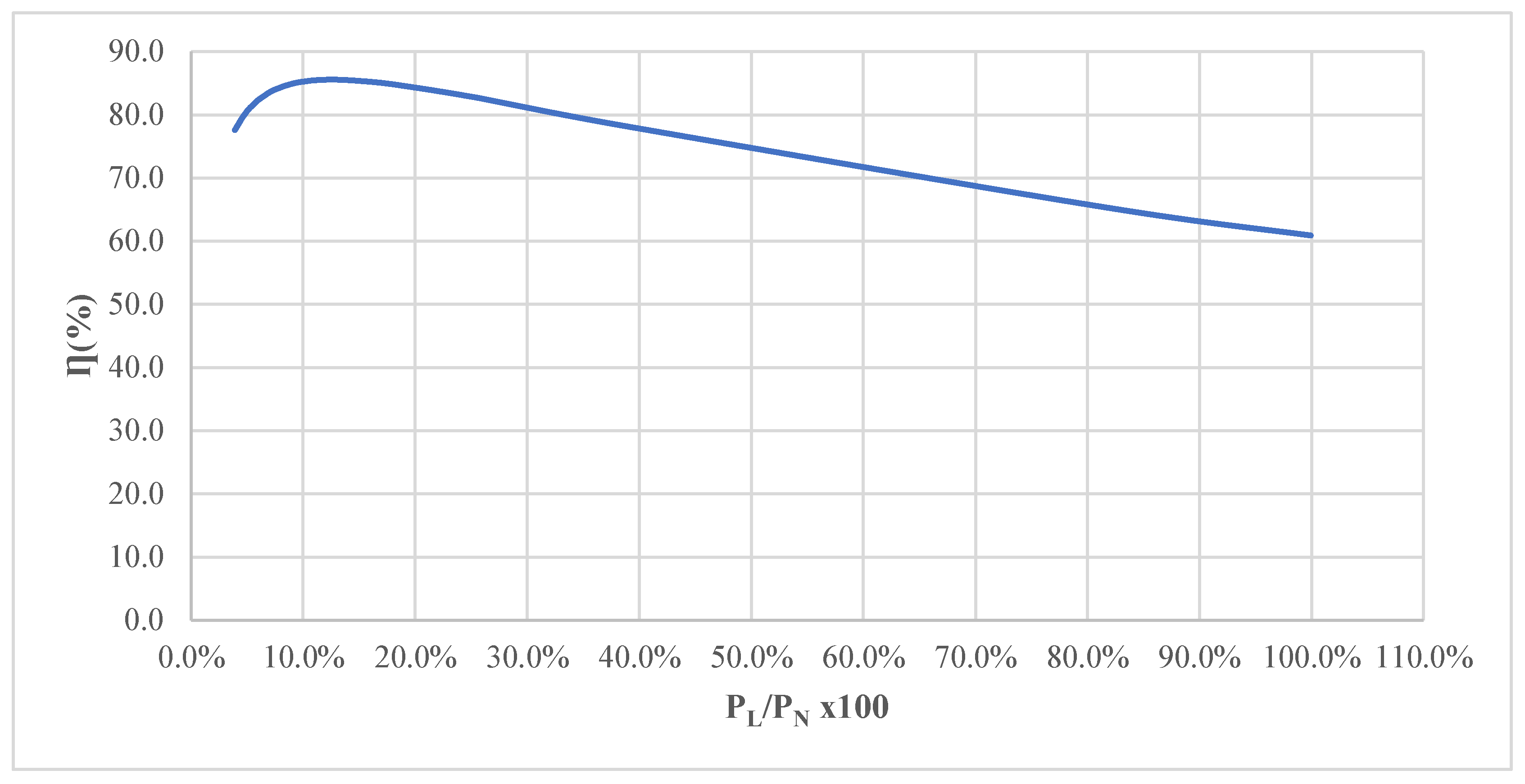
Table 5, Table 6 and Table 7 show the efficiency forecast for the transformers. From Table 5, the efficiency curve for T1 is constructed, as shown in Figure 8. Transformer T1 is forecast to have a maximum efficiency of 75% for a demand of 13.4% and 62% for a demand of approximately 50%. From a demand of 13.4%, the efficiency decreases as it approaches the nominal demand.
Figure 9 shows the efficiency curve for T2. In this case, a maximum efficiency of 85.6% occurs around a demand of 12.5%, while the minimum is estimated at a demand coefficient of 100%.
Figure 9.
Transformer efficiency curve vs demand coefficient for T2.
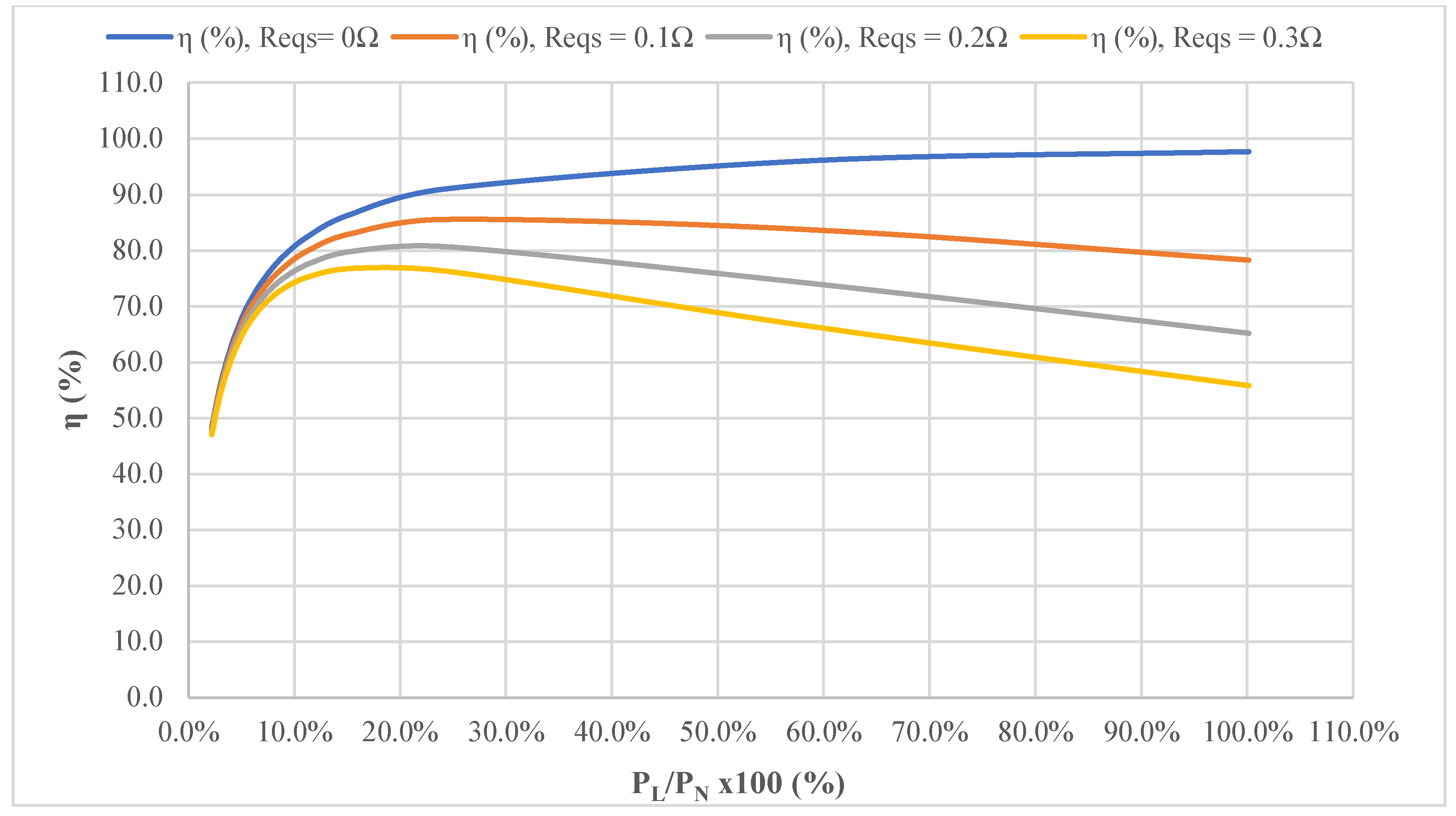
The windings of transformer T3 are of a larger gauge than those of transformers T1 and T3, so their series resistance referred to the secondary must be lower. Figure 10 shows several curves for different values of ReqS for the case of transformer T3, from a value of 0 to a value of 0.3 Ω. A high sensitivity is observed from a demand of 10% of the nominal demand. The ReqS = 0 Ω case shows an efficiency tending to 98% as the maximum demand is reached, which is not common for transformers T1 and T2, furthermore ReqS = 0 Ω is an ideal case, but it serves as a reference. For the ReqS = 0.1 Ω case, the maximum efficiency is 86.5% for a demand of 24.5%; for ReqS = 0.2 Ω, the maximum efficiency is 80.7% for a demand of 24.5%; for ReqS = 0.3 Ω, the maximum efficiency is 76.8% for a demand of 15.4%.
Figure 10.
Transformer efficiency curve vs demand coefficient for T3.
During the investigation, several limitations were presented. These limitations are related to the lack of necessary instruments and equipment. Below is a summary of the main limitations during the investigation.
- The wattmeter used does not have an independent power source, so it only measures power if the load to be measured operates in the range of 42 to 260 V. This limited the scope of the short-circuit test
- The variable alternating current source did not have sufficient capacity to feed the 1500 VA transformer, which prevented determining two of its parameters, the equivalent series resistance referred to the secondary and the equivalent series reactance referred to the secondary
- The efficiency of a transformer depends to a certain extent on the power factor, but in this work only a resistive load was used.
- The sample of transformers in terms of materials and construction, mainly represents the small autotransformers in the Dominican Republic market.
5. Conclusions and recommendations
In this work, a detailed methodology was presented to evaluate and predict the efficiency of small transformers, which are used in low voltage applications, such as inverters, battery chargers, projects, etc. In this case, transformers were used to reduce the power from 120 to 25 Vrms. The methodology included determining the parameters of the trans formers, to subsequently analytically determine the efficiency for a resistive load. These results were then compared with the actual efficiencies of each transformer for the same load. After validating the results obtained, the analytical method was used to predict the efficiency of the transformers for different resistive loads. The main results of the research are presented below.
- In the evaluation of the transformers, two of 900 VA and one of 1500 VA, efficiencies were determined in the range of 47 to 86.5%. These efficiency values are well below those of power transformers in distribution circuits, which can reach up to 98% efficiency.
- The highest efficiency of the transformers was in the demand range of 12 to 24% of the nominal demand. While the lowest efficiency was for the lowest demand.
- In general, the losses in the excitation branch or resistance in the core represent at least 90% of the losses, while the losses in the windings represent the remaining part.
Based on the results and the need for more efficient use of electrical energy in low voltage circuits in the face of growing demand worldwide, the following actions are suggested:
- Evaluate in a more exhaustive way the efficiency of low voltage transformers, for example, transformers that are in operation in different residential, commercial and industrial facilities.
- Evaluate the energy cost involved in the use of inefficient electrical transformers and economically evaluate the replacement with more efficient ones.
Funding
This rearch was funded by the financial support by the Fondo Nacional de Innovación Científico y Tecnol ógico (FONDOCYT) of the Dominican Republic, grant number 2022-3A9-140.
Acknowledgments
The author appreciates the help of engineer Carlos José Heredia, for providing part of the equipment to develop the research.
Conflicts of Interest
The author declare no conflicts of interest.
References
- Baggini, A.; Bua, F. Power transformers energy efficiency programs: A critical review. In 2015 IEEE 15th International Conference on Environment and Electrical Engineering (EEEIC), Jun. 2015, pp. 1961–1965. [CrossRef]
- Dannier and, R. Rizzo, ‘An overview of Power Electronic Transformer: Control strategies and topologies’, in Automation and Motion International Symposium on Power Electronics Power Electronics, Electrical Drives, Jun. 2012, pp. 1552–1557. [CrossRef]
- Abdullayevich, Q.N.; Qizi, Q.M.S.; O’g’li, T.A.I. Ways to Reduce Losses in Power Transformers. Tex. J. Eng. Technol. 2023, 20, 36–37. Available online: https://zienjournals.com/index.php/tjet/article/view/3955 (accessed on 5 November 2024).
- Lee, E.S.; Park, J.H.; Kim, M.Y.; Lee, J.S. High Efficiency Integrated Transformer Design in DAB Converters for Solid-State Transformers. IEEE Trans. Veh. Technol. 2022, 71, 7147–7160. [Google Scholar] [CrossRef]
- M. Alramlawi, A. M. Alramlawi, A. Gabash, and P. Li, ‘Optimal operation strategy of a hybrid PV-battery system under grid scheduled blackouts’, in 2017 IEEE International Conference on Environment and Electrical Engineering and 2017 IEEE Industrial and Commercial Power Systems Europe (EEEIC / I CPS Europe), Jun. 2017, pp. 1–5. [CrossRef]
- El-Dabah, M.A.; Agwa, A.M. Identification of Transformer Parameters Using Dandelion Algorithm. Applied System Innovation 2024, 7, 5. [Google Scholar] [CrossRef]
- chased, ‘Electromagnetism’, Smithsonian Institution Archives. Available online: https://siarchives.si.edu/history/featured-topics/henry/electromagnetism (accessed on 6 November 2024).
- Guarnieri, M. Who Invented the Transformer? IEEE Industrial Electronics Magazine 2013, 7, 56–59. [Google Scholar] [CrossRef]
- Maurice George Say, Alternating Current Machines. Pitman Publishing; 5th Revised edition (January 1, 1984), 1984.
- S. J. Chapman, Máquinas eléctricas, 4th ed. México: McGraw Hill, 2005.
- CarvalElectronics, ‘CALIBRES DE ALAMBRE DE COBRE | CarvalElectronics’. Available online: https://www.carvalelectronics.com/producto/calibres-de-alambre-de-cobre (accessed on 6 November 2024).
- wattmeter, ‘AC 80-260V 100A LCD Digital Display Multi-Function Power Monitor Voltage Current Frequency Power Factor Energy Meter Ammeter Voltmeter with Split Core Current Transformer: Amazon.com: Tools & Home Improvement’. Available online: https://www.amazon.com/80-260V-Multi-Function-Frequency-Voltmeter-Transformer/dp/B0CC51H1B8?pd_rd_w=7wkHT&content-id=amzn1.sym.c388ca75-4c14-4d9d-947d-5dcde63263f5&pf_rd_p=c388ca75-4c14-4d9d-947d-5dcde63263f5&pf_rd_r=MTSCGJKF27RVWNKMWJ5A&pd_rd_wg=McVgL&pd_rd_r=07ee69ef-6a3a-4d16-a101-252994b016e8&pd_rd_i=B0CC51H1B8&psc=1&ref_=pd_bap_d_csi_prsubs_1_i (accessed on 6 November 2024).
Figure 1.
Basic diagram of an ideal electrical transformer. Source: own elaboration.
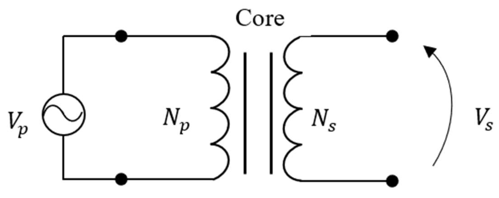
Figure 2.
Approximate models of transformers. (A) Referring to the primary side; (B) Referring to the secondary side. Source: Own elaboration.
Figure 2.
Approximate models of transformers. (A) Referring to the primary side; (B) Referring to the secondary side. Source: Own elaboration.
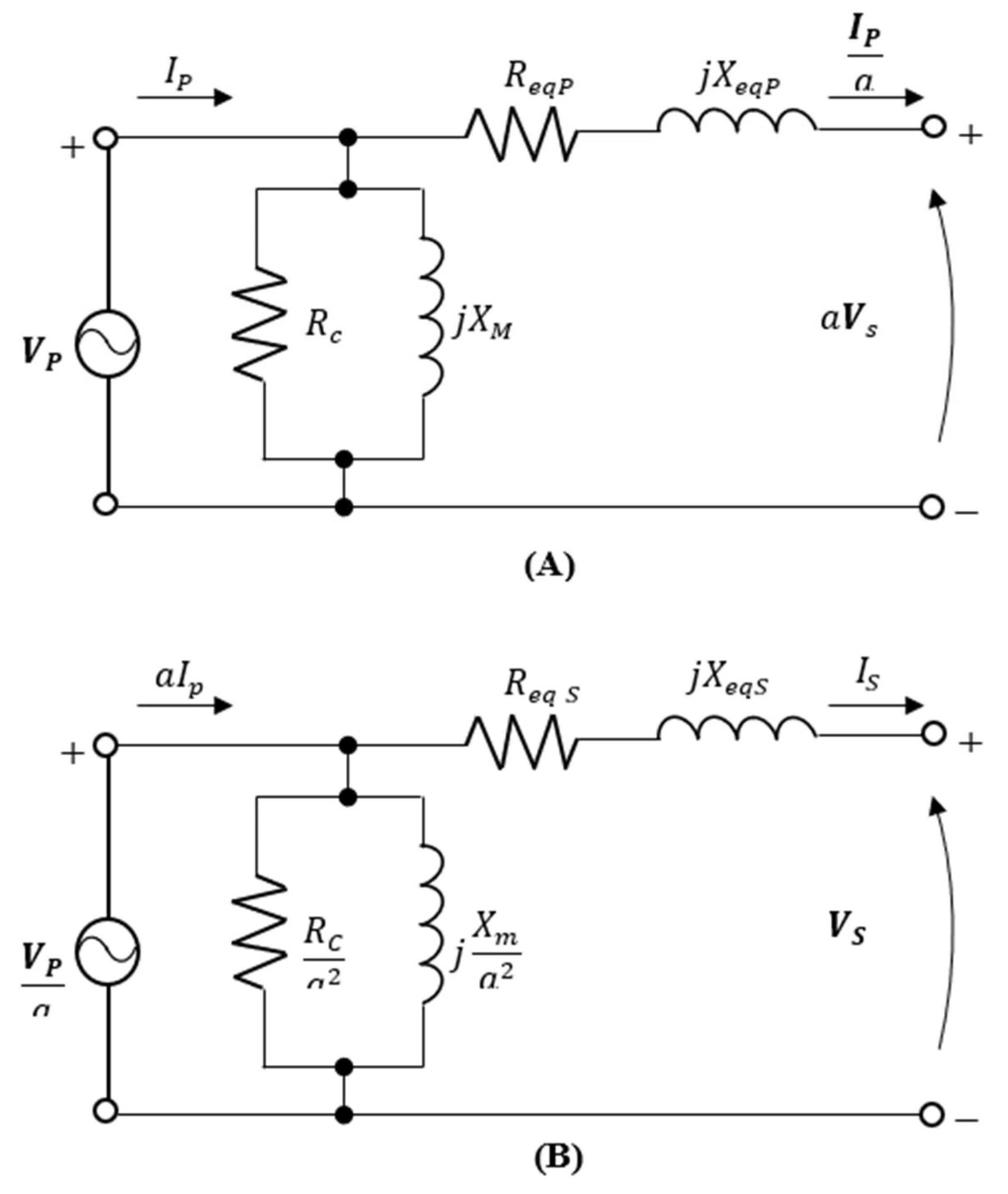
Figure 3.
Connection diagram for open circuit test.
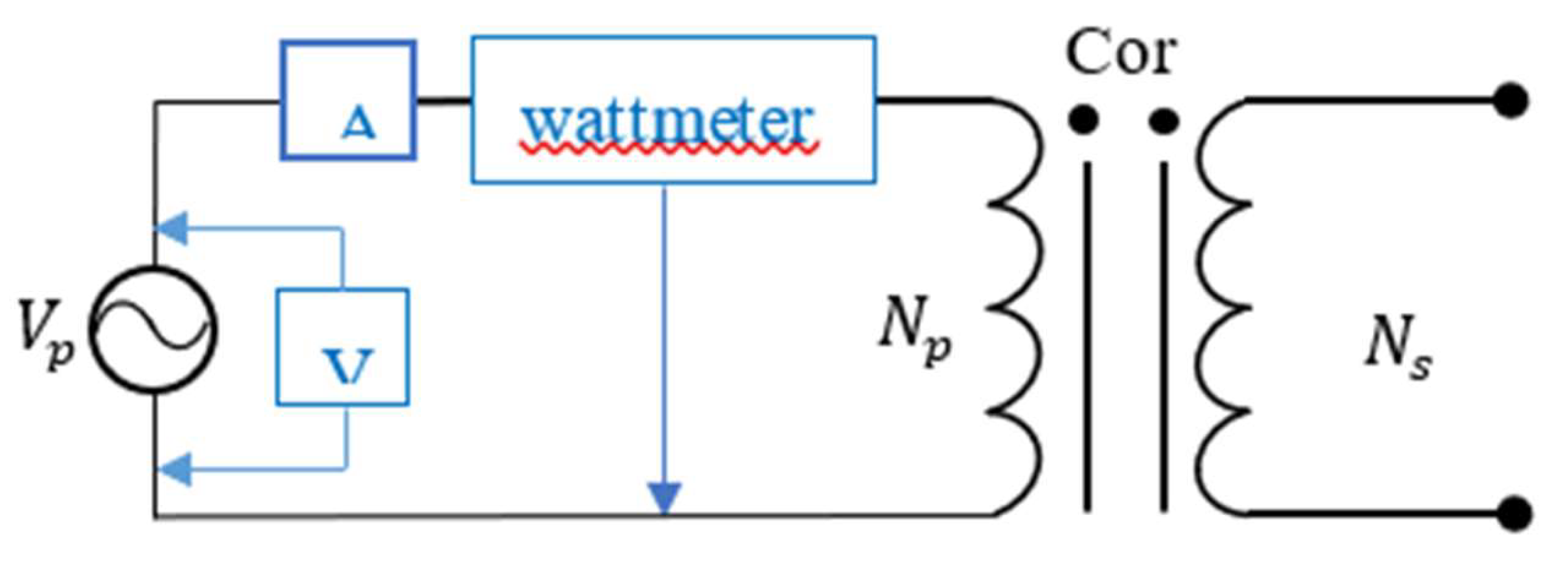
Figure 4.
Esquema de conexión para la prueba de cortocircuito.
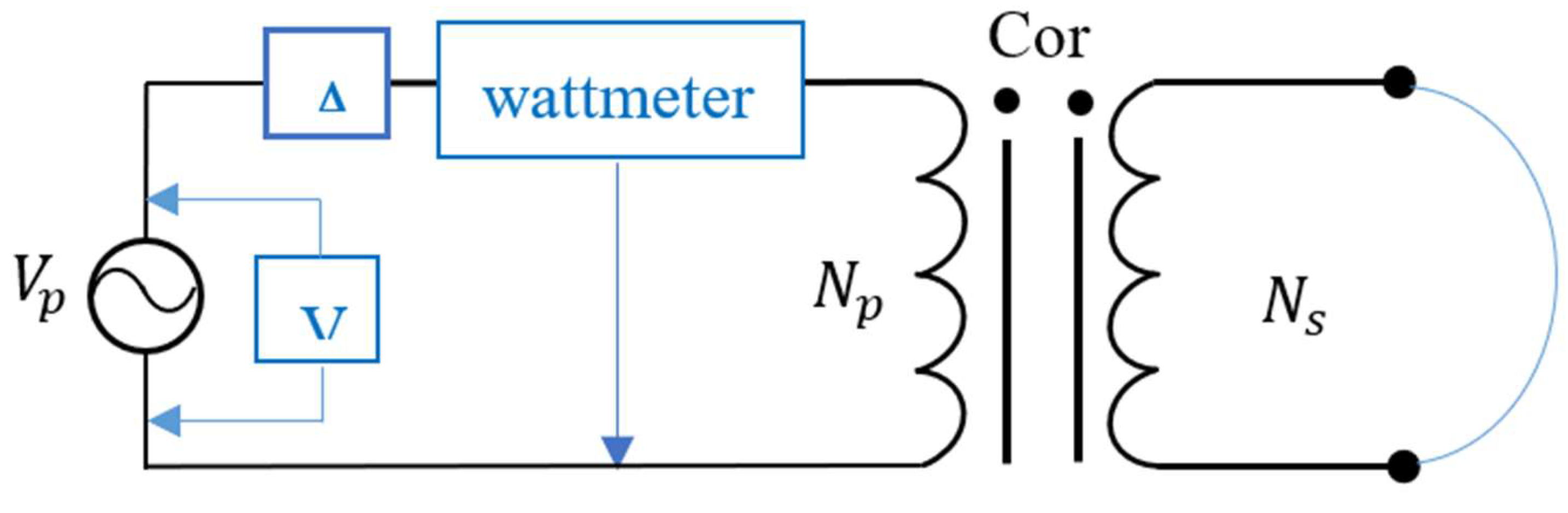
Figure 5.
The three small transformers for the case study. T1): transformer made by students in a technical high school; T2: transformer of a project; T3: transformer of an electrical inverter.
Figure 5.
The three small transformers for the case study. T1): transformer made by students in a technical high school; T2: transformer of a project; T3: transformer of an electrical inverter.
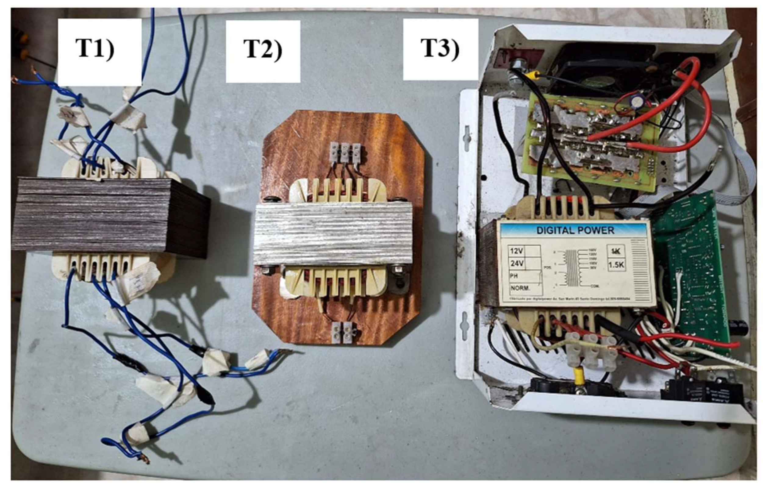
Figure 6.
Instruments and apparatus used in the tests: A) Variable AC source; B) AC wattmeter; C) AC ammeter and voltmeter; D) electrical load.
Figure 6.
Instruments and apparatus used in the tests: A) Variable AC source; B) AC wattmeter; C) AC ammeter and voltmeter; D) electrical load.
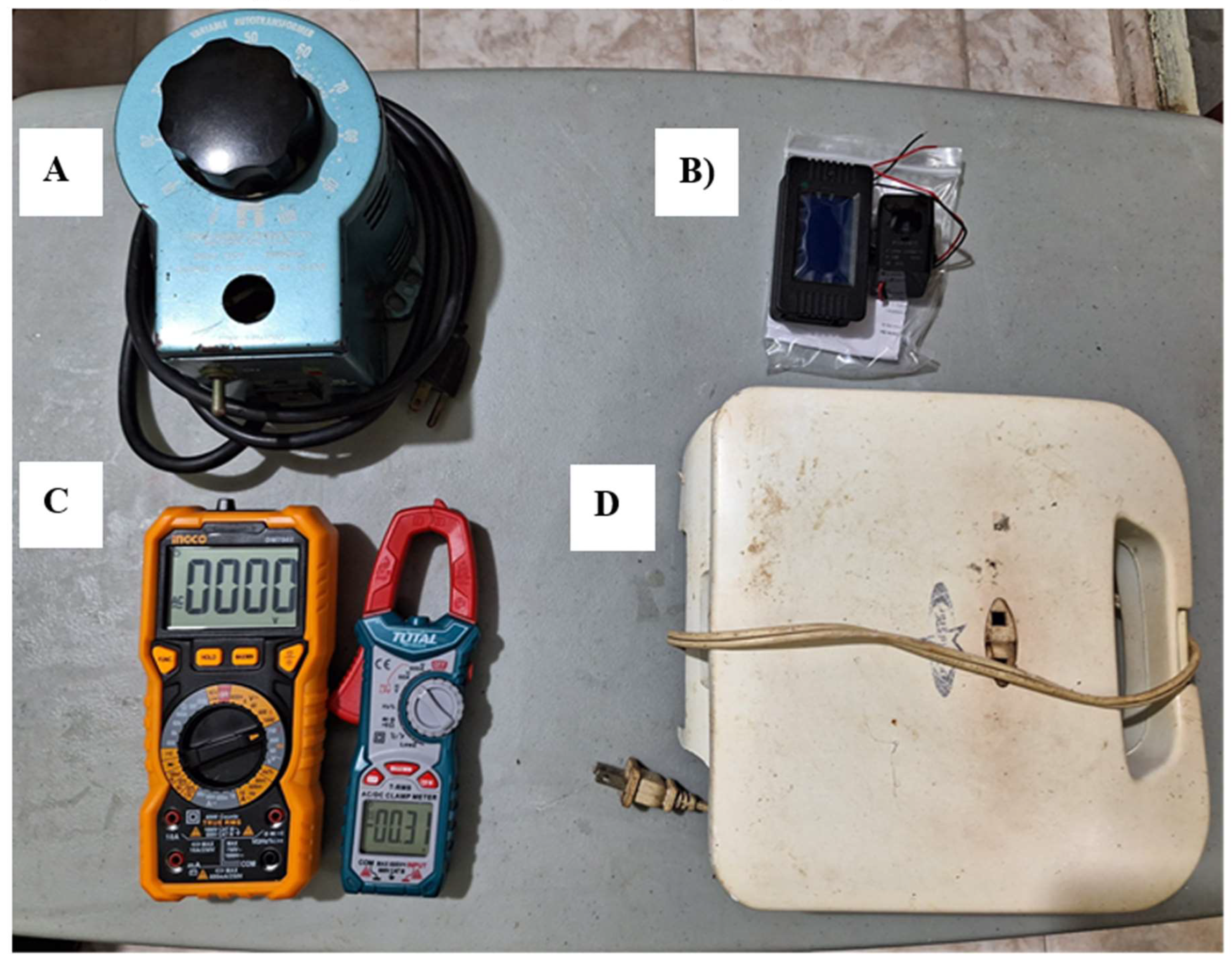
Figure 7.
Figure 7. Flowchart of the methodology used to develop the research
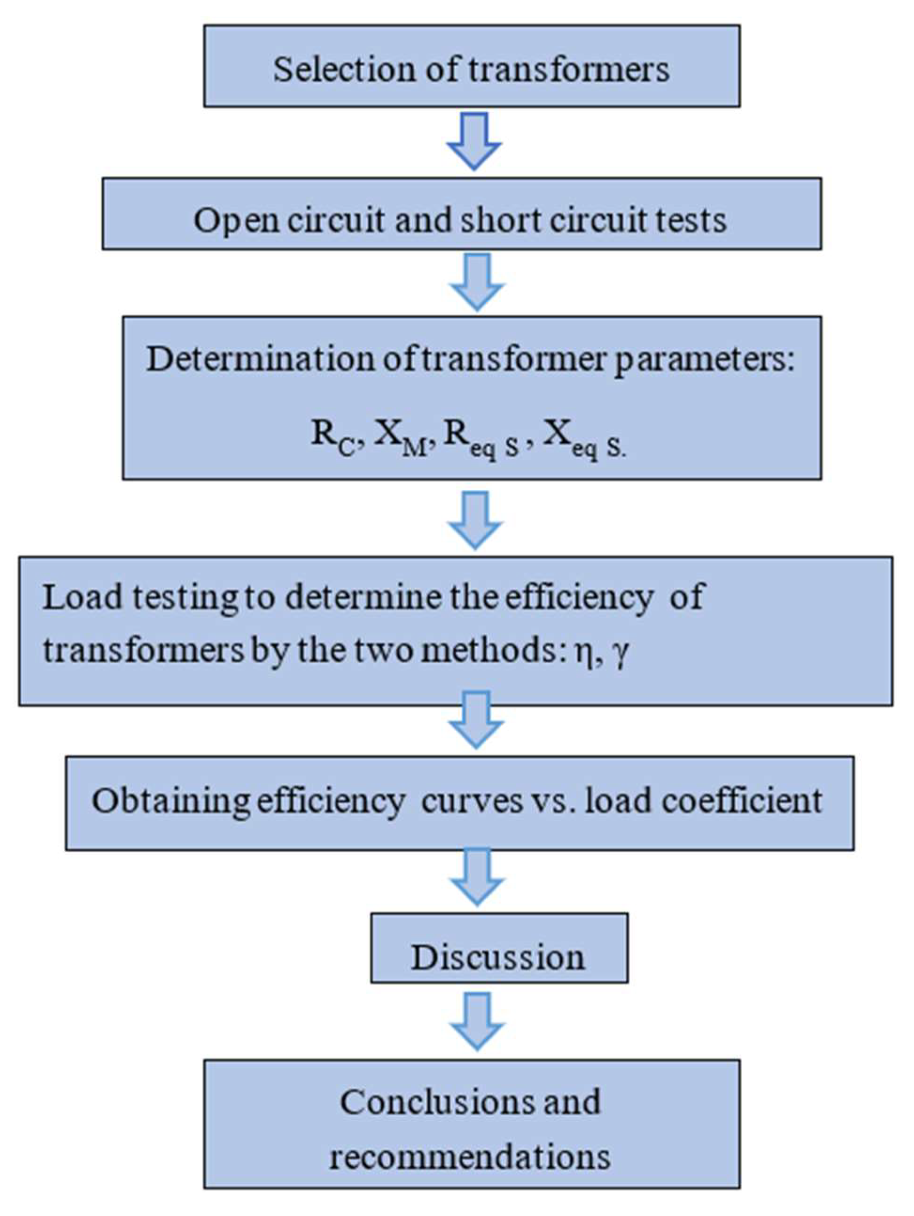
Figure 8.
Connection images for the two tests on transformer T1: A) open circuit test; B) short circuit test when the operating voltage range of the wattmeter has not been reached; C) short circuit test with the wattmeter measuring.
Figure 8.
Connection images for the two tests on transformer T1: A) open circuit test; B) short circuit test when the operating voltage range of the wattmeter has not been reached; C) short circuit test with the wattmeter measuring.
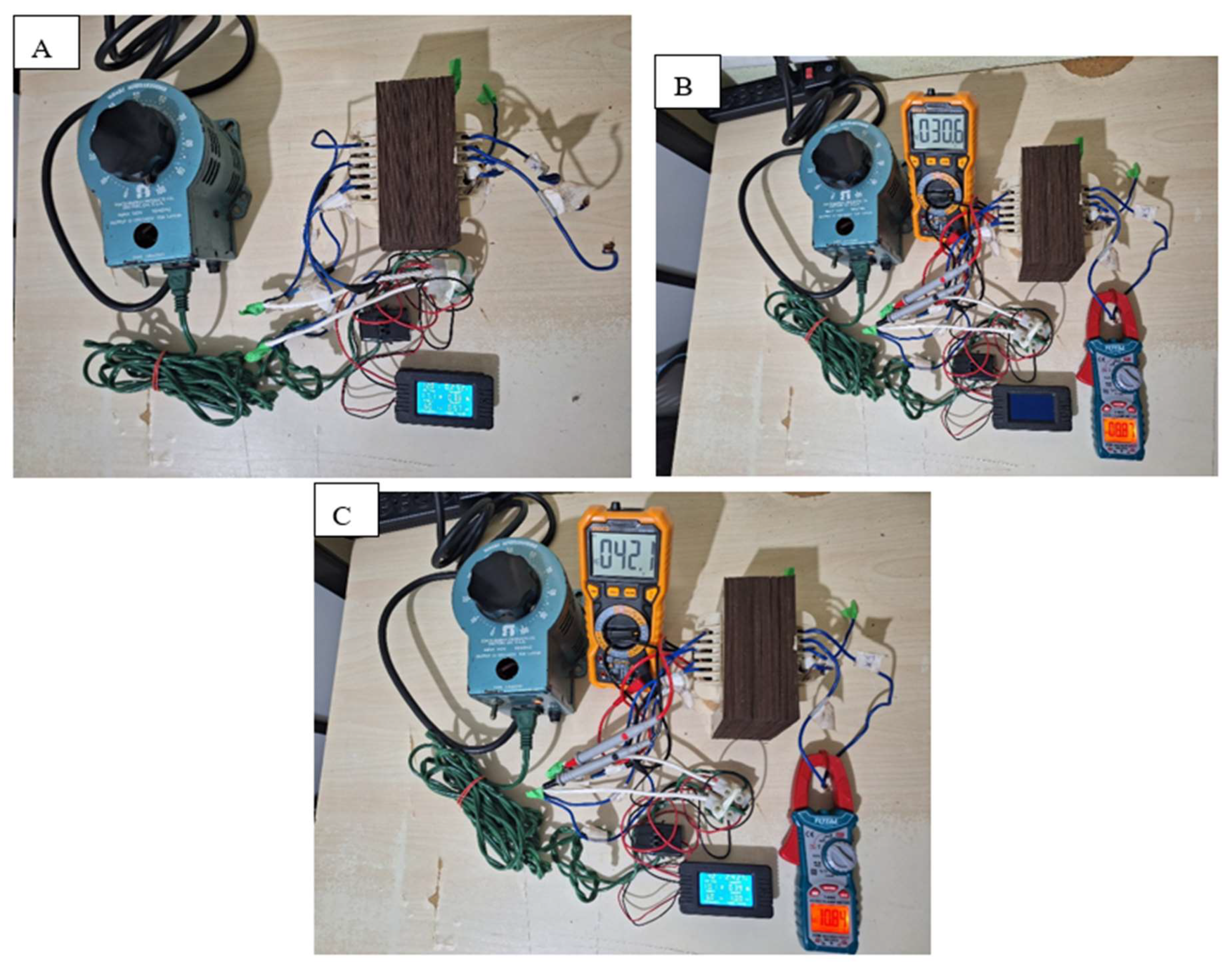
Figure 9.
Connection images for the two tests on transformer T2: A) open circuit test; B) short circuit test.
Figure 9.
Connection images for the two tests on transformer T2: A) open circuit test; B) short circuit test.
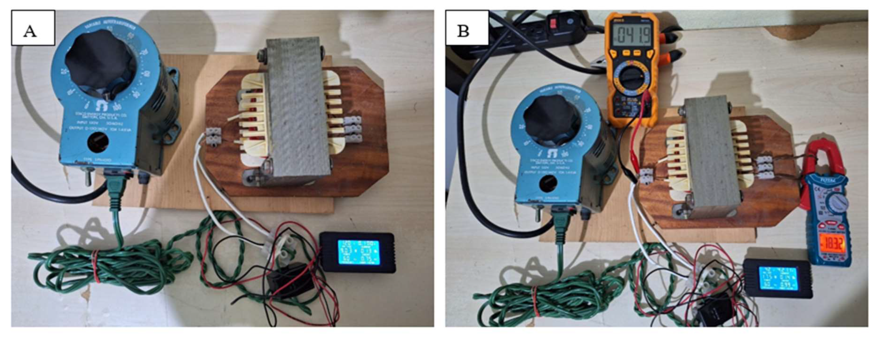
Figure 10.
Connection images for the two tests on transformer T3: A) open circuit test; B) short circuit test.
Figure 10.
Connection images for the two tests on transformer T3: A) open circuit test; B) short circuit test.
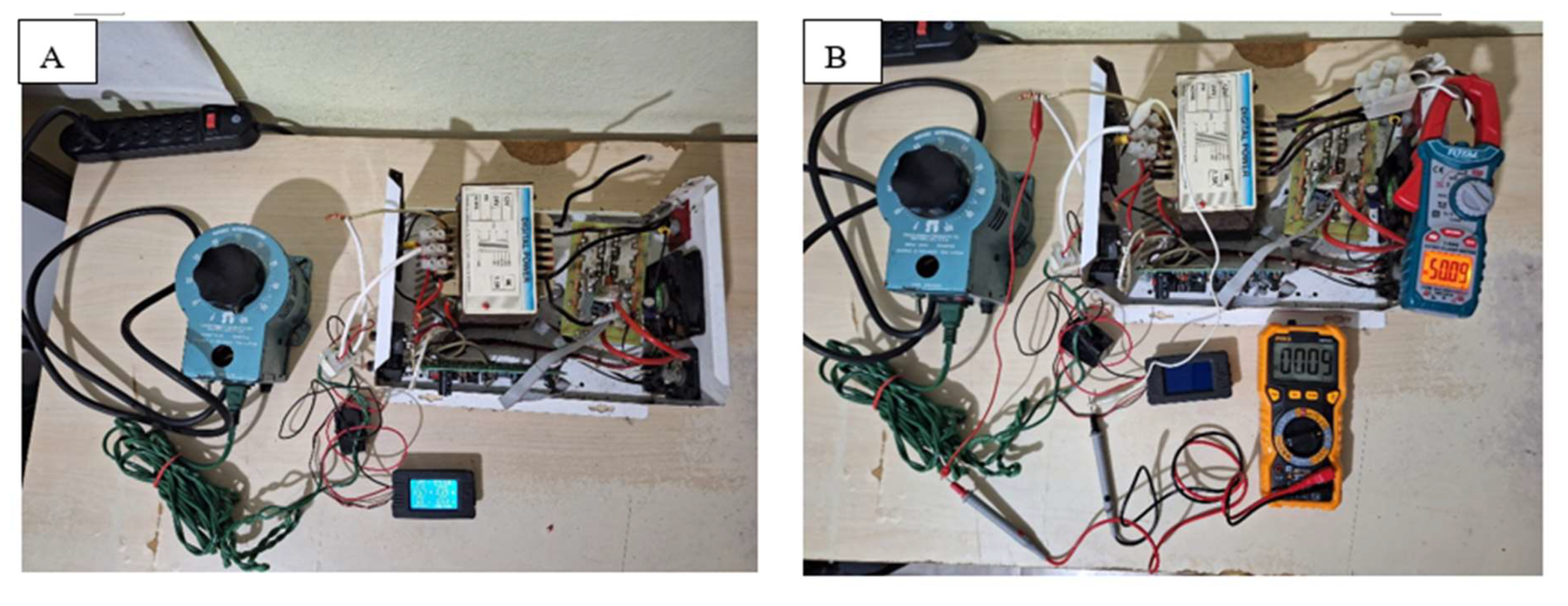
Figure 11.
Approximate circuit model referring to the secondary for T1. Source: own elaboration.
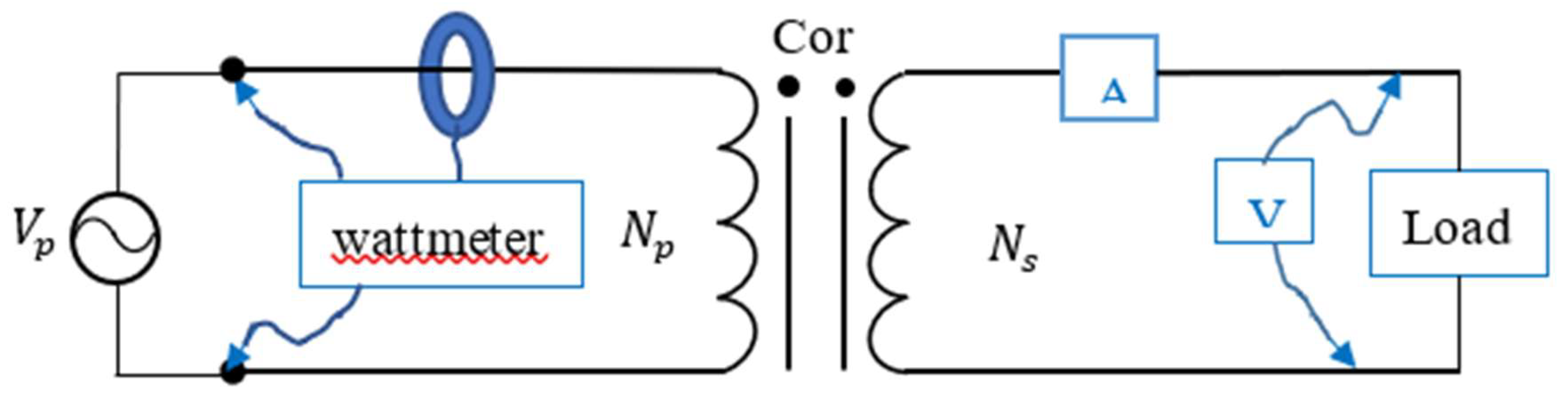
Figure 12.
Connections to determine efficiency under load. A) connection for T1; B) connection for T2; connection for T3.
Figure 12.
Connections to determine efficiency under load. A) connection for T1; B) connection for T2; connection for T3.
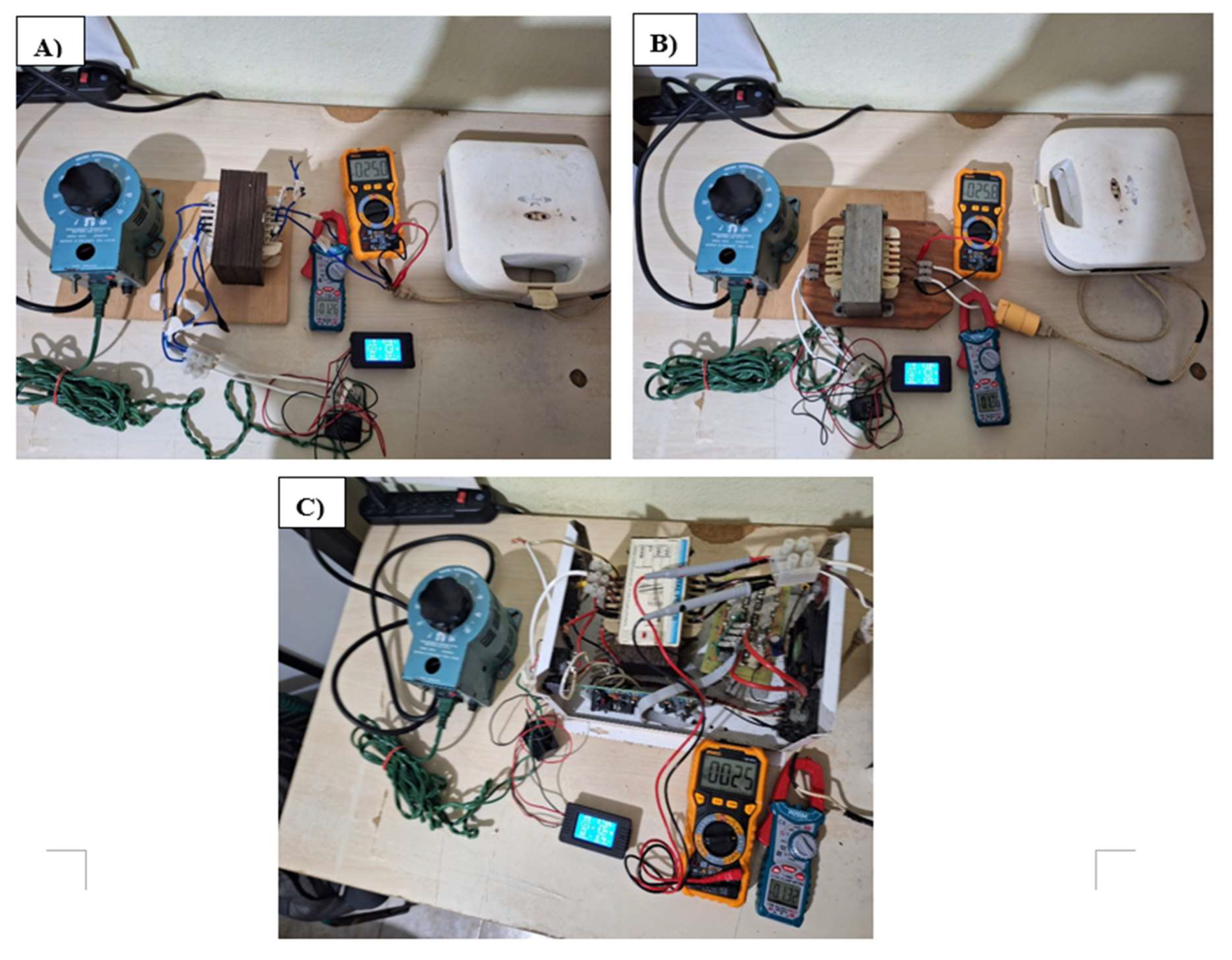
Figure 8.
Transformer efficiency curve vs demand coefficient for T1.
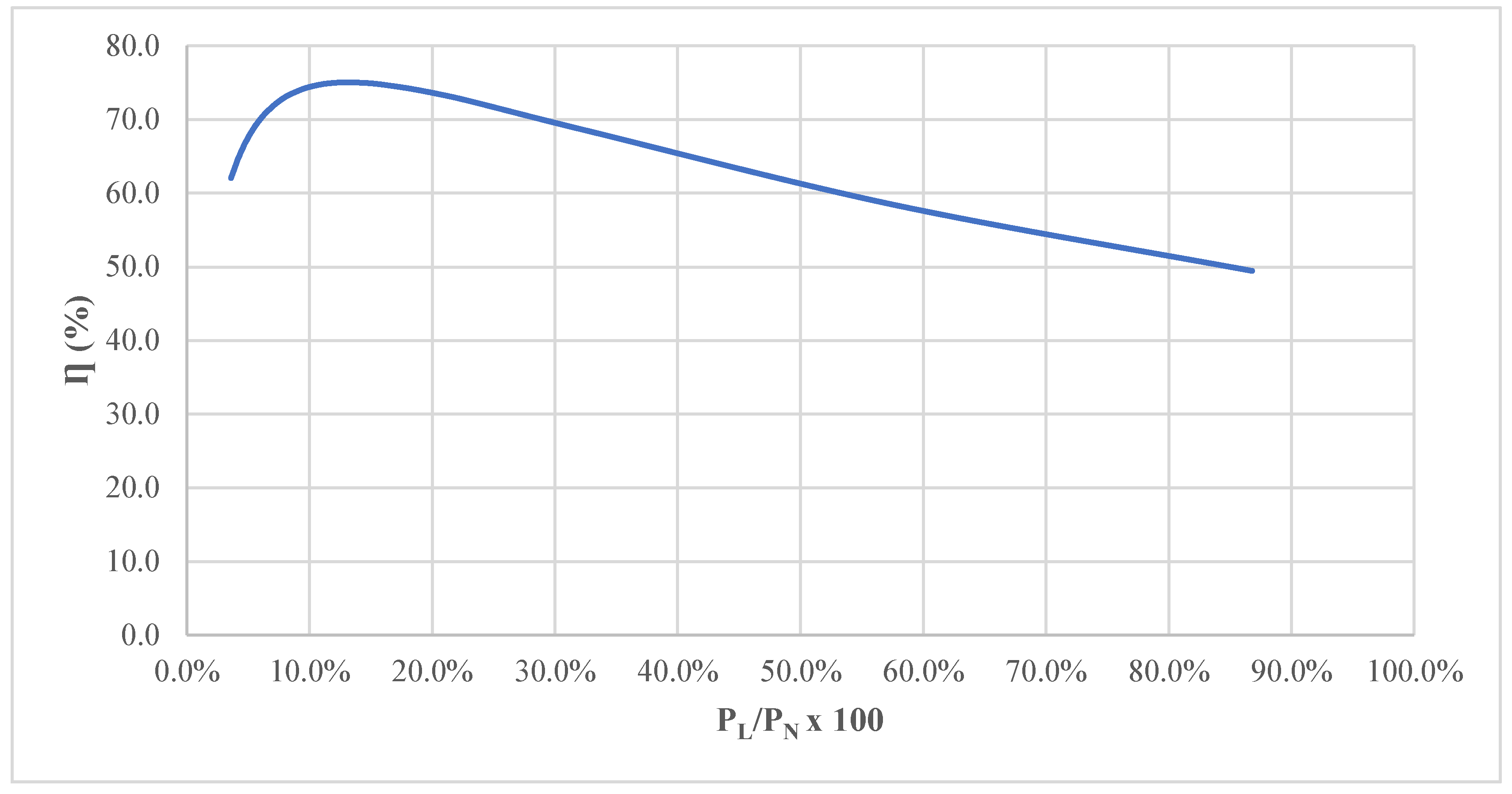

Table 1.
Data from the three selected transformers.
| Data | Transformers | ||
|---|---|---|---|
| T1 | T2 | T3 | |
| A (cm2) | 30.0 | 30.0 | 39 |
| S (VA) | 900 | 900 | 1500 |
| Bm (Gauss) | 9500 | 9500 | 9500 |
| Vp (V) | 120 | 120 | 120 |
| a | 4.80 | 4.65 | 4.80 |
| dP (mm), wire #, Amapacity (A) | 1.44, 15, 6.60 | 1.58, 14, 8.30 | 1.80, 13, 10.50 |
| dS (mm), wire #, Amapacity (A) | 0.72, 21, 1.62 | 1.58, 14, 8.30 | 4.32, 6, 53.16 |
Table 2.
Open circuit and short circuit test results.
| Measured data | |||
|---|---|---|---|
| Open circuit test | T1 | T2 | T3 |
| IA (A) | 0.252 | 0.100 | 0.569 |
| VA (V) | 120 | 120 | 120 |
| PA (W) | 17.1 | 9.03 | 35.8 |
| PF= PA/ VAIA | 0.570 | 0.752 | 0.524 |
| Short circuit test | |||
| ISC (A) | 2.427 | 4.211 | -- |
| VSC (V) | 42.1 | 42.0 | -- |
| PSC (W) | 101 | 175 | -- |
| PF= PC/ VCIC | 1.00 | 1.00 | - - |
| Additional data | |||
| Short circuit current in the secondary: ISC s (A) | 10.84 | 18.32 | -- |
Table 3.
Calculated parameters, referring to the primary and secondary of each transformer.
| Calculated parameters referred to the primary | T1 | T2 | T3 |
|---|---|---|---|
| RC (Ω) | 835 | 1.60 x10³ | 402 |
| XM (Ω) | 580 | 1.82 x10³ | 248 |
| Req P (Ω) | 17.3 | 9.87 | -- |
| Xeq P (Ω) | 0.00 | 1.26 | -- |
| Calculated parameters referred to the secondary | |||
| RC S= RC /a2 (Ω) | 36.2 | 74.0 | 17.4 |
| XM /a2 (Ω) | 25.2 | 84.2 | 10.7 |
| Req S=Req P/a2 (Ω) | 0.751 | 0.456 | -- |
| Xeq S = XeqP /a2 (Ω) | 0.000 | 0.0583 | -- |
Table 4.
Load test results to determine efficiency.
| Required parameters | T1 | T2 | T3 |
|---|---|---|---|
| PP (W) | 52.0 | 45.4 | 72.5 |
| IS (A) | 1.29 | 1.36 | 1.32 |
| VS (V) | 25.0 | 25.8 | 25.0 |
| PS (W)= VS x IS | 32.2 | 35.1 | 33.0 |
| γ (%) = PS / PP x100 | 61.9 | 77.3 | 45.5 |
Table 5.
Efficiency vs. T1 demand coefficient.
| RL (Ω) | IS (A) | PL | PL/PN | η (%) |
|---|---|---|---|---|
| 18.4 | 1.30 | 32.6 | 3.6% | 62.0 |
| 17.4 | 1.37 | 34.3 | 3.8% | 63.0 |
| 16.4 | 1.45 | 36.3 | 4.0% | 64.1 |
| 15.4 | 1.54 | 38.6 | 4.3% | 65.1 |
| 14.4 | 1.64 | 41.1 | 4.6% | 66.1 |
| 13.4 | 1.76 | 44.0 | 4.9% | 67.2 |
| 12.4 | 1.89 | 47.3 | 5.3% | 68.3 |
| 11.4 | 2.05 | 51.2 | 5.7% | 69.4 |
| 10.4 | 2.23 | 55.8 | 6.2% | 70.5 |
| 9.4 | 2.45 | 61.3 | 6.8% | 71.5 |
| 8.4 | 2.72 | 67.9 | 7.5% | 72.5 |
| 7.4 | 3.05 | 76.2 | 8.5% | 73.4 |
| 6.4 | 3.47 | 86.8 | 9.6% | 74.2 |
| 5.4 | 4.03 | 100.8 | 11.2% | 74.8 |
| 4.4 | 4.81 | 120.2 | 13.4% | 75.0 |
| 3.4 | 5.95 | 148.8 | 16.5% | 74.6 |
| 2.4 | 7.81 | 195.3 | 21.7% | 73.0 |
| 1.4 | 11.4 | 284.1 | 31.6% | 68.9 |
| 0.4 | 20.8 | 520.8 | 57.9% | 58.4 |
| 0 | 31.3 | 781.3 | 86.8% | 49.5 |
Table 6.
Efficiency vs T1 demand coefficient.
| RL (Ω) | Is (A) | PL | PL/PN | η (%) |
|---|---|---|---|---|
| 18.4 | 1.37 | 35.2 | 3.9% | 77.6 |
| 17.4 | 1.44 | 37.2 | 4.1% | 78.3 |
| 16.4 | 1.53 | 39.4 | 4.4% | 79.0 |
| 15.4 | 1.62 | 41.9 | 4.7% | 79.8 |
| 14.4 | 1.73 | 44.7 | 5.0% | 80.5 |
| 13.4 | 1.86 | 47.9 | 5.3% | 81.2 |
| 12.4 | 2.00 | 51.6 | 5.7% | 82.0 |
| 11.4 | 2.17 | 55.9 | 6.2% | 82.7 |
| 10.4 | 2.37 | 61.1 | 6.8% | 83.3 |
| 9.4 | 2.61 | 67.2 | 7.5% | 84.0 |
| 8.4 | 2.90 | 74.8 | 8.3% | 84.6 |
| 7.4 | 3.27 | 84.3 | 9.4% | 85.0 |
| 6.4 | 3.74 | 96.5 | 10.7% | 85.4 |
| 5.4 | 4.37 | 112.8 | 12.5% | 85.6 |
| 4.4 | 5.27 | 135.8 | 15.1% | 85.4 |
| 3.4 | 6.62 | 170.7 | 19.0% | 84.6 |
| 2.4 | 8.90 | 229.5 | 25.5% | 82.7 |
| 1.4 | 13.6 | 350.3 | 38.9% | 78.2 |
| 0.4 | 28.7 | 739.6 | 82.2% | 65.2 |
| 0.24 | 34.9 | 899.5 | 99.9% | 60.9 |
Table 7.
Efficiency vs. demand coefficient of T3. Since ReqS could not be determined, several curves are made for the values 0, 0.1, 0.2 and 0.3 of ReqS.
Table 7.
Efficiency vs. demand coefficient of T3. Since ReqS could not be determined, several curves are made for the values 0, 0.1, 0.2 and 0.3 of ReqS.
| PL (W) | PL/PN | η (%), ReqS = 0 Ω | η (%), ReqS = 0.1 Ω | η (%), ReqS = 0.2 Ω | η (%), ReqS = 0.3 Ω |
|---|---|---|---|---|---|
| 33.4 | 2.2% | 48.2 | 47.8 | 47.4 | 47.0 |
| 35.3 | 2.4% | 49.6 | 49.2 | 48.7 | 48.3 |
| 37.4 | 2.5% | 51.0 | 50.6 | 50.1 | 49.7 |
| 39.8 | 2.7% | 52.6 | 52.1 | 51.6 | 51.1 |
| 42.5 | 2.8% | 54.2 | 53.7 | 53.1 | 52.6 |
| 45.6 | 3.0% | 55.9 | 55.4 | 54.8 | 54.2 |
| 49.2 | 3.3% | 57.8 | 57.2 | 56.5 | 55.9 |
| 53.4 | 3.6% | 59.8 | 59.1 | 58.4 | 57.7 |
| 58.4 | 3.9% | 61.9 | 61.1 | 60.4 | 59.6 |
| 64.4 | 4.3% | 64.2 | 63.3 | 62.4 | 61.6 |
| 71.8 | 4.8% | 66.7 | 65.7 | 64.7 | 63.7 |
| 81.2 | 5.4% | 69.3 | 68.2 | 67.0 | 65.9 |
| 93.3 | 6.2% | 72.2 | 70.8 | 69.5 | 68.3 |
| 109.6 | 7.3% | 75.3 | 73.7 | 72.1 | 70.6 |
| 133.0 | 8.9% | 78.7 | 76.7 | 74.8 | 73.0 |
| 168.9 | 11.3% | 82.5 | 79.9 | 77.5 | 75.2 |
| 231.5 | 15.4% | 86.6 | 83.1 | 79.8 | 76.8 |
| 367.6 | 24.5% | 91.1 | 85.6 | 80.7 | 76.2 |
| 892.9 | 59.5% | 96.1 | 83.7 | 74.0 | 66.2 |
| 2083.3 | 100.2% | 97.7 | 78.3 | 65.2 | 55.8 |
Table 8.
Percentage error between the analytical method and the experimental method.
| Transformer | γ (%) | ƞ (%) | Er = (ƞ- γ)x100/ γ |
|---|---|---|---|
| T1 | 61.9 | 61.9 | 0 % |
| T2 | 77.3 | 77.4 | 0.129 % |
| T3 | 45.5 | 48.3 | 6.15 % |
Disclaimer/Publisher’s Note: The statements, opinions and data contained in all publications are solely those of the individual author(s) and contributor(s) and not of MDPI and/or the editor(s). MDPI and/or the editor(s) disclaim responsibility for any injury to people or property resulting from any ideas, methods, instructions or products referred to in the content. |
© 2024 by the authors. Licensee MDPI, Basel, Switzerland. This article is an open access article distributed under the terms and conditions of the Creative Commons Attribution (CC BY) license (http://creativecommons.org/licenses/by/4.0/).
Copyright: This open access article is published under a Creative Commons CC BY 4.0 license, which permit the free download, distribution, and reuse, provided that the author and preprint are cited in any reuse.


