Submitted:
18 November 2024
Posted:
19 November 2024
You are already at the latest version
Abstract
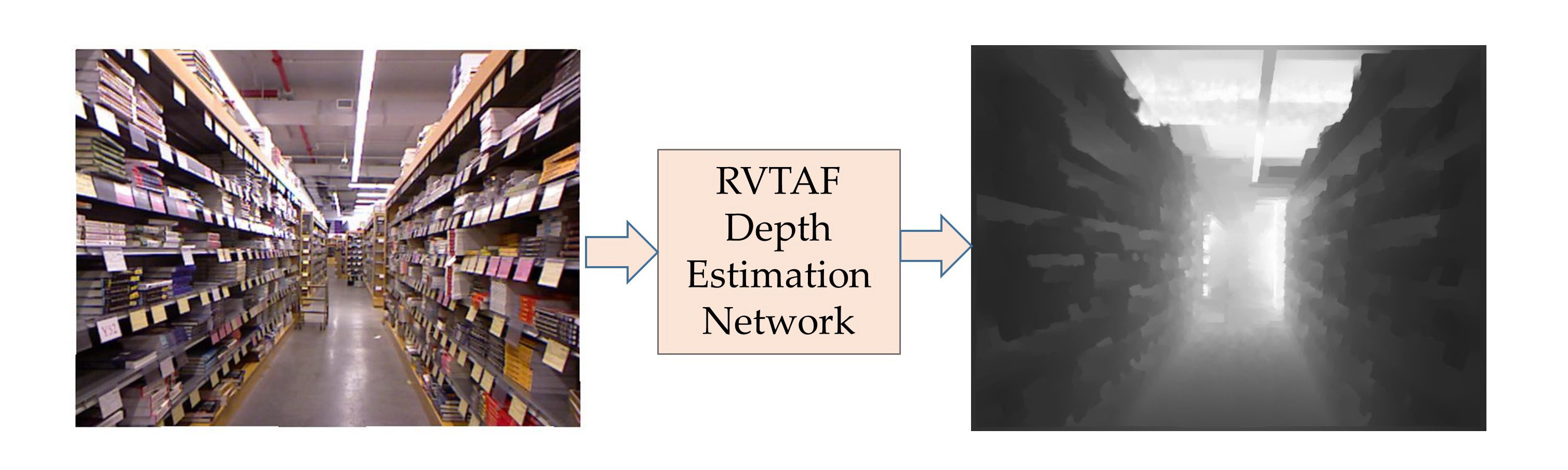
Precision depth estimation plays a key role in many applications, including 3D scene reconstruction, virtual reality, autonomous driving and human-computer interaction. Recent advancements in deep learning technologies, the monocular depth estimation has surpassed the traditional stereo camera systems, bringing new possibilities in 3D sensing. In this paper, by using single camera, we propose an end-to-end supervised monocular depth estimation autoencoder which contains a CNN-ViT encoder and an adaptive fusion decoder, to obtain high-precision depth maps. In the CNN-ViT encoder, we construct a multi-scale feature extractor by mixing residual configurations of vision transformers to enhance both local and global information. In the adaptive fusion decoder, we introduce adaptive fusion modules to effectively merge features of the encoder and decoder together. Lastly, the model is trained using a loss function that aligns with human perception to enable it to focus on the depth values of foreground objects. Experimental results demonstrate the effective prediction of the depth map from a single-view color image by the proposed RVTAF autoencoder.
Keywords:
monocular depth estimation
; convolutional neural networks
; residual vision transformer
; adaptive fusion
; autoencoder
1. Introduction
The purpose of depth estimation is to accurately predict the distance between objects and the camera lens. Depth information finds wide application across various fields, including household robots [1], autonomous driving [2], 3D movie production [3], etc. The depth information could be also the input data for other computer vision tasks such as face recognition [4], object detection [5] and semantic segmentation [6]. A high-quality depth map is mostly characterized by accurate depth values specified along the well-defined object boundaries.
Depth estimation was originally started from stereo matching techniques [7,8,9,10] in uses of two or more cameras. If we try to use a single view image to predict the depth, it becomes a challenging task due to its ill-posed condition. When humans try to understand the spatial relationship of the objects in a view single image, they consider both local cues and global context. Local cues refer to the details as the texture appearance and the perspective of objects, the relative sizes, etc. On the other hand, global context referring to occlusion issues, could be exhibited from the layout of the scene. By assessing these factors, humans can make good sense of the geometric configuration from a single image.
For deep learning networks, various feature extractors, which have been proposed to retrieve the detailed image features, employ a series of convolutional neural and down-sampling blocks to gradually extract the detailed to overall feature layer-by-layer. For instance, VGG [11] achieves this by applying multiple 3×3 convolution layers and pooling operations to encode the image. For better convergence, ResNet [12] utilizes residual blocks with skip connections to learn residual information and extract image features. For both VGG and ResNet, the features in the shallow layers possess more detailed information while those in deeper layers hold more global information. In recent years, vision transformers [13] have gained a lot of attention because of achieving good performance in computer vision tasks. Many researchers attribute this success to the self-attention mechanism [14], which enables the input features to capture abundant global information and significantly expand their receptive fields. However, the amounts of parameters and calculations of the vision transformer are very large. In addition to the final extracted features, we must efficiently utilize the detailed features from lower layers by the co-called skip connections [15]. How to perfectly fuse the decoded feature and the skip connection feature is crucial in the decoder.
2. Related Work
Monocular depth estimation (MDE) [16], which is accomplished by using just a single color image, can significantly minimize the requirement for multiple cameras and greatly reduce hardware resources. Since monocular depth estimation methods only take a single color image as the input, they are more difficult than the stereo matching approaches to estimate the precision depth map. The monocular depth estimation methods with deep learning structures can be divided into supervised and unsupervised learning approaches. Supervised networks apply ground truth depth maps to train a neural network as a regression model. Eigen et al. [17] were the pioneers to approach monocular depth estimation using deep learning method, where the CNN-based network comprises two stacked deep networks, a coarse depth network and a refinement network. As to the unsupervised monocular depth estimation, Godard et al. [18] introduced a network system that takes a single view image as the input to generate depth map without ground truth depth. During the training period, however, it needs both the left and right views. The input left and right view images with the estimated depth maps by the MDE networks are respectively warped to the other synthesized view images. The reconstruction loss subsequently utilizes the closeness of the synthesized and the input images to facilitate unsupervised learning. Considering consecutive multiple single view frames, Yang et al. [19] suggested video-based depth estimation autoencoder to further improve the performances.
2.1. Vision Transformer
Dosovitskiy et al. [13] are the pioneers for developing structure related to transformer in image classification task. Vision transformer (ViT) [13], which is a new type of neural network for computer vision, extends the success of transformers originally developed for natural language processing [14]. The ViT and its variations have gained significant attentions and achieved state-of-the-art results in various computer vision tasks such as image classification [20], semantic segmentation [21] and depth estimation [22] with higher computation. Unlike traditional convolutional neural networks (CNNs) that rely on spatial convolutions and pooling layers, vision transformers utilize the self-attention mechanism to calculate global dependencies and long-range relationships within an image.
In vision transformers, the input image is segmented into patches, which are then flattened to vectors. Linear projection or 1×1 convolution is used for adjusting the length of the flattened vectors as “patch embeddings” or “tokens”. These tokens are then passed through transformer blocks to capture global information. The basic architecture of vision transformer block is shown in Figure 1. The vision transformer consisted layer normalization, multi-head self-attention, channel MLP and residual connections.
2.2. Atrous Spatial Pyramid Pooling
For expanding the receptive field, a common solution is to increase the kernel size of standard convolutions. However, the computation might become larger while using a bigger convolutional kernel size. Dilated convolution is similar to standard convolution by introducing gaps between each kernel pixel based on the specific dilation rate. This allows the kernel receptive field to be expanded without increasing computations. For instance, in a standard 3×3 convolution with dilation rate 2, its receptive field is expanded to achieve the same receptive field as a standard 5×5 standard convolution kernel. The 3×3 convolution with dilation rate 2 utilizes only 9 kernel parameters.
2.3. Selective Feature Fusion
To effective fuse the skip connection features, GLPDepth [16] utilizes selective feature fusion (SFF) modules to achieve high quality depth as shown in Figure 3. Instead of element-wise summation of skip connection and decoder features, the SFF module offers improved fusion capabilities. It is noted that the skip connection feature FSC and the decoder feature FD are with the size of C×H×W. They are first concatenated along the channel dimension and then passed through two layers of 3×3 convolution, batch normalization, and ReLU and finally gone through a 3×3 convolution layer to reduce the number of channels to 2, and undergo sigmoid activation function to obtain two attention maps, ASC and AD. By performing element-wise multiplications of FSC to ASC and FD to AD, these weighted features are element-wise added together to construct the final fused feature FF.
3. Proposed Methods
For monocular depth estimation, effectively combining the local information and the global features is an important challenge to estimate the depth map with exceptional quality. As shown in Figure 4, the basic framework of the proposed residual vision transformer and adaptive fusion (RVTAF) depth estimation network consists of a CNN-ViT encoder and an adaptive fusion decoder. The CNN-ViT encoder is further composed of an CNN feature extractor mixed with several ViT modules to extract local and global features, while the multiple level features are skip connected to fuse the feature of the decoder to achieve high quality depth estimation. In the RVTAF depth estimation network, we need to identify a better residual configuration of vision transformers to successfully expand the receptive field of the bottleneck feature. We also need to design an effective adaptive fusion module (AFM) to further enhance the precision of the estimation. The detailed explanation of the CNN-ViT encoder and adaptive fusion decoder are present in the following two subsections.
3.1. CNN-ViT Encoder
The detailed structure of the final CNN-ViT encoder, which is shown in Figure 5, mainly contains subsampled residual blocks (SRBs) and residual blocks (RBs) to extract 3 mid-level features and the bottleneck feature with the size of 512xH/16xW/16. By experiments, the proposed CNN-ViT encoder incorporated vision transformers (ViTs), which are marked in yellow color, of course, should be further discussed later. Inspired by ResNet50 [12], the backbone is constructed by two different building blocks to become the CNN feature extractor. The detailed structures of subsampled residual block (SRB) and residual block (RB) are shown as follows.
3.1.1. Subsampled Residual Block
As shown in Figure 6, the subsampled residual block (SRB) is with two branches, where the lower branch first projects the input feature to a lower dimension space by 1×1 convolution by half. Then the spatial information will be further down-sampled through a 3×3 convolution with stride 2, and finally the features will be projected to twice dimension of the input feature with 1×1 convolution. The upper branch first uses a max-pooling operation to achieve down-sampling the spatial information by half and follows by a 1×1 convolution to obtain the originally down-sampled feature. Finally, the features from these two branches are combined through element-wise summation to obtain the output feature. The height and width of the input feature (CxHxW) is reduced to half while the channel number is increased twice for the output feature (2CxH/2xW/2).
3.1.2. Residual Block
As shown in Figure 7, the residual block (RB) employs a 1×1 convolution to reduce the dimension of the input feature by half. Once the feature is projected into the low-dimensional space, we utilize a 3×3 convolution with a stride of 1 to capture spatial information. Following that, a 1×1 convolution is used to adjust the dimension to match that of the input feature. Finally, we combine the learned feature with the input feature through element-wise summation. The output feature of the residual block (RB) maintains the same feature size as the input feature.
3.1.3. Vision Transformer
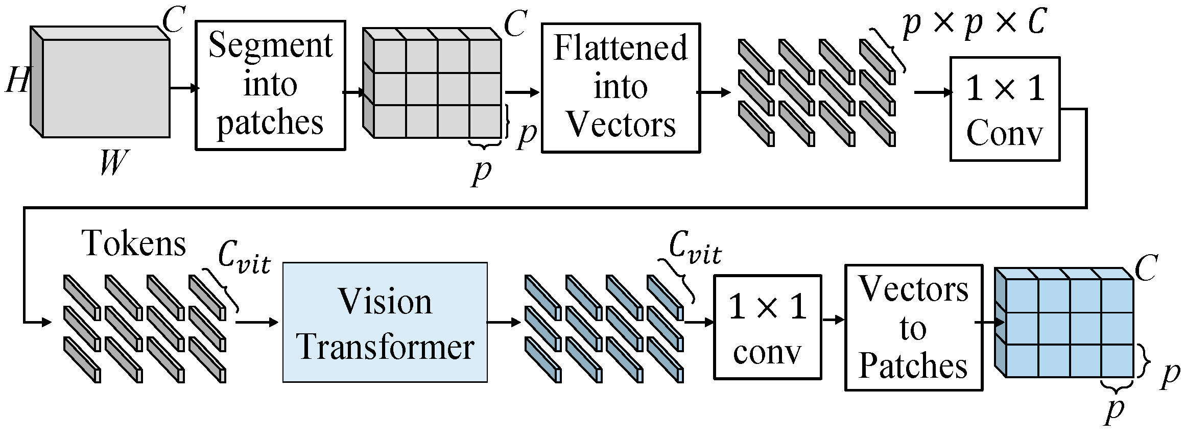
The flow chart of the realized vision transformer is shown in Figure 8. The input feature map is segmented into patches with size of p×p, where we set p = 5. These patches are flattened into vectors then followed by a 1×1 convolution to adjust the length of vectors to Cvit. We call these adjusted vectors “patch embeddings”, which have the size of Cvit×1×1. After the preparation of the inputs for vision transformer, these patch embeddings are sent into the vision transformer, which is shown in Figure 1(b), to learn global information. After vision transformer, the patch embeddings, which have the size of Cvit×1×1, learn a lot of global information. we deploy a 1×1 convolution to adjust the lengths of learned patch embeddings from Cvit to p×p×C. Then, as the flattened procedure, we reverse the process and restore the learned patch embeddings back to their original size. Follow the procedure we designed, we can obtain a feature, which has rich global information, learned by vision transformer. The feature with global information has the same size as the input feature.
Figure 9.
Flow chart of the realized vision transformer.
There are many ways to insert vision transformers (ViTs) into the CNN encoder. Initially, we attempted to add vision transformers to each feature extraction stage in a sequential manner, however it does not refine details of depth quality. To mitigate the impact of vision transformer on the shallow layers, we proposed a residual layout of the vision transformers into each feature extraction stage as shown in Figure 10, where we mark five positions (Position 1, Position 2, …., Position 5) for adding (n1, n2…., n5) ViTs, respectively. With the limited 5 ViTs, i.e., n1+n2+n3+n4+n5 = 5 for reasonable computation complexity, we will determine the best configurations of these five ViTs in the CNN network by experiments in Section 4.
3.2. Adaptive Fusion Decoder
To achieve a good decoder, we believe that feature fusion of skip connections will be the crucial design to achieve an effective autoencoder. The decoder layer could refer the detailed information of the encoder, which progressively extracts layer features with a global scope. Consequently, effectively integrating the skip connection feature extracted from the encoder with the decoded feature returned by the decoder becomes an indispensable concern. The structure of the adaptive fusion decoder as shown in Figure 11 is composed of up-conversion (Upconv) blocks, fusion modules (FMs) and a Deep ASSP module. We will explain the in the following subsections.
There are many ways to fuse two features together. To improve the SFF module [16], we suggest three variants of the fusion module (FM), namely separate enhancement addition fusion module (SEAFM), separate enhancement concatenation fusion module (SECFM) and adaptive fusion module (AFM). We believe that the skip connection feature and the decoded feature have their distinct feature characteristics, which implies that the attention maps ASC and AD cannot be generated using the same set of weights and need to be extracted separately. The detailed explanations of these three fusion modules are present as follows.
3.2.1. Separate Enhancement Addition Fusion Module
As shown in Figure 12, the separate enhancement addition fusion module (SEAFM) independently enhances the two input features. The skip connection feature branch and the decoded feature branch undergo two sequential 3×3 convolution-batch normalization-ReLU layers, reducing the number of channels to one-fourth of the original. Subsequently, a 3×3 convolution operation further decreases the channel to 1. Finally, the attention map ASC for the skip connection feature branch and the attention map AD for the decoded feature branch are obtained through a Sigmoid operation. By element-wise multiplication of ASC with the feature of the skip connection branch (FSC) and AD with the feature of the decoded branch (FD), the resulting weighted feature is obtained. The two weighted features are then combined through element-wise summation to yield the final hybrid fused feature (FF).
3.2.2. Separate Enhancement Concatenation Fusion Module
As shown in Figure 13, the separate enhancement concatenation fusion module (SECFM), which is a modified version of the SEAFM, is modified the addition operation of the SEAFM with the concatenation operation of two weighted features, which are then further processed by a 3×3 convolution-batch normalization-ReLU operation. Of course, the element-wise summation in the SEAFM is slightly more efficient and requires fewer parameters than the concatenation in the SECFM.
3.2.3. Adaptive Fusion Module
As shown in Figure 14, the adaptive fusion module (AFM) first concatenates the skip connection feature and the decoded feature before being split into two branches for attention map generations. This approach ensures that both branches have accessed the information from two features, thereby enhancing the generation process with more comprehensive and integrated information. By incorporating this strategy, the attention maps SAC and AD can effectively prioritize crucial information from both features, leading to improved performance. In contrast, the generation process of the two attention maps in SEAFM is independent, lacking knowledge of the information present in the other map. The adaptive fusion module with the observation of two inputs to generate attention maps through two different branches. These two attention maps will be adaptively generated for the two distinct features.
3.2.4. Up Convolution Module
We deploy up-convolution (Upconv) blocks to increase the width and height of the decoded feature and fused features while reducing the number of channels. This step ensures that the feature not only matches the input size of the subsequent AFM but also enhances the precision of spatial information in the up-sampled feature. The architecture of the up-convolution block is shown in Figure 15. The input feature of the up-convolution block will first up-sampling to double their width and height, then pass through a layer of 3×3 convolution-batch normalization-ReLU for enhancing the spatial information.
3.2.5. Deep ASPP Module
When the dilation rate exceeds the width and height of the feature, dilated convolution behaves similarly to a 1×1 convolution. Consequently, the output of certain branches in the ASPP module will not extend to the receptive field. To improve the Atrous spatial pyramid pooling (ASPP) [23,24], we deploy the Deep ASPP [25], which was used for segmentation task, to help the model to expand its receptive field of the feature. Unlike the original ASPP, the Deep ASPP possesses a much wider receptive field, and prevents the degradation of Atrous convolution kernels with high dilated rates into 1×1 convolution. We put Deep ASPP module after the first fusion module (FM) as shown in Figure 14. Because the feature at here is far from the output head, in other words, it is in the deep location in the autoencoder. The architecture of Deep ASPP module is shown in Figure 16
3.3. Training Loss Function
In order to calculate the distance between predicted depth map and ground truth depth map D, we use a scale-invariant log loss [17] to train the proposed network. The training loss function is given as:
with
where and represent the ground truth depth map and predicted depth map of the ith pixel, respectively. In (1), the loss function is calculated with square-mean minus mean-square, as known as the variance when α=1. When α = 0, the loss function becomes an L2 loss. Here, we set α =0.5 to train our network as suggested in [17].
During the network training process, we normalize the ground truth depth values to a range between 0 and 1. This normalization allows the network to predict depth values within the same range during regression. By applying the logarithm function as shown in Figure 16 to the difference between two values ranging from 0 to 1, the error is effectively amplified specially for low values. This amplification has a stronger impact on smaller ground truth depth values. As a result, our predicted depth map prioritizes the accurate prediction of foreground depth values. This amplification helps in improving the accuracy of our predicted depth values. It is important to highlight that during the training process with the KITTI dataset, we exclusively consider pixels where and for calculating the loss function. This approach is adopted because logarithms of depth values cannot be defined when the depth is 0. By focusing on non-zero depth values, we prevent difficulties that may arise during training.
4. Experimental Results
The proposed RVTAF depth estimation network is implemented by using Python 3.6 with Pytorch [27] 1.10.2. For hardware systems, we used a personal computer with Intel Core i7-7700K CPU and NVIDIA GeForce RTX 3070Ti 8G GPU. To validate the effectiveness of our approach, we present several experimental results on challenging benchmarks that encompass diverse settings. Specifically, we provide experimental results on two famous benchmarks, which encompass both indoor and outdoor environments.
The NYU Depth V2 dataset [24] consists of 120K image-depth pairs obtained from video sequences captured using a Microsoft Kinect. The images have a size of 480×640 and are collected from 464 indoor scenes. For training our network, we utilize approximately 50K training pairs obtained from random crops of size 416×544. We evaluate the performance of our approach on 654 testing pairs at full resolution. The depth maps have an upper bound of 10 meters. The two selected image-depth pairs in the NYU Depth V2 dataset are shown in Figure 17.
Speaking of outdoor scene, the KITTI dataset [28] is a widely recognized in the field of depth estimation. The KITTI dataset comprises 61 scenes from various categories such as “city”, “residential”, “road”, and “campus”. To ensure fair comparisons with existing methods, we adopt the split proposed by Eigen et al. [17] for the training and testing. Therefore, we evaluate our approach on a subset of 652 images across 29 scenes, while the remaining 32 scenes consisting of 23,488 images are used for training purposes. The RGB images have a resolution of approximately 376×1241, whereas the corresponding depth maps exhibit low density and contains numerous missing data points. Therefore, we calculate the loss function only for those of the depth map that have valid values. Two selected image-depth pairs in the KITTI dataset are shown in Figure 18. The images will be uniformly cropped to a fixed size of 352×1216 at a specific position. Afterwards, we train our network using a random crop of size 352×704. During evaluation, we utilize the full resolution with the size of 352×1216.
To prevent overfitting during network training, we employ several data augmentation techniques. For both the KITTI dataset and NYU Depth v2 dataset, we utilize random cropping. For the NYU Depth v2 dataset, we crop the images to a size of 416×544 during training and perform inference with the full-size images, which are 480×640. For the KITTI dataset, we crop the images to a size of 352×704 and perform inference with a size of 352×1216. Additionally, each image has a 50% chance of being horizontally flipped. We also apply random adjustments to the brightness, saturation, and hue of each image. These data augmentation methods introduce variability into the training set, effectively reducing the risk of overfitting.
For training, we utilize the Adam optimizer [29] with cosine decay. We adopt the 1-cycle policy for the learning rate, where max_lr is set to 1e-4. We apply linear warm-up from max_lr/10 to max_lr for the first 10% of iterations followed by cosine decay to 3e-5. The total number of epochs is set to 150, with a batch size 6, except for the ablation study, which is trained for approximately 70 epochs.
4.1. CNN-ViT Encoder with Various ViT Configurations
First, we conducted extensive experiments to determine the optimal positioning of vision transformers (ViTs) combined into the CNN encoder, the most reasonable configurations are enlisted in Table 1. To reduce the computation, we only test the patterns with more ViTs for the deeper-level features, which could achieve better results and less computation. Each configuration is denoted by five digits, n1 n2 n3 n4 n5, which represent the specific numbers of ViTs used in Positions 1, 2, 3, 4, 5, respectively as illustrated in Figure 10. For “00000” case, it is noted that the no ViT module are used, of course, the computation becomes the least. For “00131”, it indicates that there are no ViTs in Positions 1 and 2, one ViT in Position 3, three ViTs in Position 4, and one ViT in Position 5. The simulation results show that the position indices, “01121” has the best estimation performance. However, we prefer to choose the position indices “00023”, which has near quality as “01121”, due to low complexity consideration. Thus, as shown in Figure 5, we should choose 2 ViTs in Position 4 and 3 ViTs in Position 5 to achieve the overall best performance.
4.2. Adaptive Fusion Decoder with Various Fusion Modules
In the previous chapter, we provided a detailed introduction to the baseline method SFF [16] as well as three fusion modules we suggested. Now, we conducted comparative analyses of the baseline and the proposed fusion modules as the subsequent ablation study. To ensure a fair comparison of their performance, we utilized the same model architecture for all four fusion modules, only replacing the specific fusion component. The results in Table 2 clearly demonstrate that adaptive fusion module (AFM), which concatenates the skip connection feature and the decoded feature and generates attention maps through two separate branches, consistently outperforms the other fusion modules across all evaluation metrics. Of course, the AFM with concatenated data and separate branches requires higher number of parameters.
4.3. Comparisons on NYU Depth V2 Dataset
In this experiment, we utilized the NYU Depth V2 test set, specifically 654 samples, to evaluate the performance of the three models. Table 3 clearly demonstrates that our proposed RVTAF depth estimation network outperforms the other two methods across all evaluation metrics. Figure 20 shows two test images and their ground truth depth maps while Figure 21 shows the visualization comparisons of depth estimation results comparing with the existing approaches. The proposed RVTAF depth estimation network in figures all achieves better depth results than the BTS [26] and GLPdepth [16] methods in NYU Depth V2 dataset.
4.4. Comparisons on KITTI Dataset
In this experiment, we utilized the KITTI dataset Eigen split, which contains 652 testing images. In Table 5, it is evident that our proposed RVTAF network surpasses GLPDepth in all metrics, particularly in the δ1 metric, where the proposed RVTAF network demonstrates similar performance, with a slight edge over the BTS.
Figure 22 shows visualization comparisons of depth estimation results achieved by the proposed and the existing approaches in KITTI dataset. The proposed RVTAF network in figures also exhibits better depth results than the BTS and GLPDepth methods.
5. Conclusions
In this paper, we proposed a residual vision transformer and adaptive fusion (RVTAF) depth estimation network that is based on an autoencoder with skip connection architecture. In the proposed encoder, we suggest a residual configuration of CNN-based feature extractor to effectively integrate vision transformers (ViTs) to achieve better performance. As for the proposed decoder, we introduce the adaptive fusion module (AFM) to effectively fuse the skip connection feature from the encoder with the decoded feature, where the AFM generates two attention maps, allowing each feature to concentrate on specific spatial information. Additionally, we enhanced the decoder portion by incorporating a deep ASPP module to expand the effective receptive field of deep features. Ultimately, the proposed RVTAF depth estimation network is capable of accurately predicting depth maps from single image. We conducted multiple ablation studies to determine a configuration that uses less parameters and maintains better performance for the vision transformer (ViT) and evaluate the effectiveness of our proposed adaptive fusion module (AFM). Subsequently, we compared our final network with existing methods for both indoor scenes on NYU Depth V2 dataset and outdoor scenes on KITTI dataset Eigen split. In the case of indoor scenes, our method achieves sharper boundaries and more accurate depth values. Additionally, our network successfully captures depth information from traffic signs and vehicles in the KITTI dataset. Overall, the experimental results demonstrate that our method is competitive with current methods.
Author Contributions
Conceptualization, W.Y. C.W. and J.Y; methodology, W.Y.; software, C.W.; validation, W.Y. C.W. and J.Y.; formal analysis, W.Y..; investigation, W.Y.; resources, W.Y.; data curation, W.Y. and C.W.; writing—original draft preparation, C.W. and W.Y.; writing—review and editing, W.Y. and J.Y.; visualization, W.Y.; supervision, W.Y.; project administration, W.Y.; funding acquisition, W.Y. All authors have read and agreed to the published version of the manuscript.
Funding
This research was funded by the National Science and Technology Council, Taiwan under Grant: NSC 111-2222-E-167 -005.
Institutional Review Board Statement
Not applicable.
Informed Consent Statement
Not applicable.
Conflicts of Interest
The authors declare no conflicts of interest.
References
- F. Fabrizio and A. De Luca, "Real-time computation of distance to dynamic obstacles with multiple depth sensors," IEEE Robotics and Automation Letters, vol. 2, no. 1, pp. 56-63, Jan. 2017, doi: 10.1109/LRA.2016.2535859. [CrossRef]
- O. Natan and J. Miura, "End-to-end autonomous driving with semantic depth cloud mapping and multi-agent," IEEE Trans. on Intelligent Vehicles, vol. 8, no. 1, pp. 557-571, Jan. 2023, doi: 10.1109/TIV.2022.3185303. [CrossRef]
- P. Kauff, N. Atzpadin, C. Fehn, M. Müller, O. Schreer, A. Smolic and R. Tanger, “Depth map creation and image-based rendering for advanced 3DTV services providing interoperability and scalability,” Signal Processing: Image Communication, vol. 22, no. 2, February 2007, pp.217-234. [CrossRef]
- Gaile G. Gordon, "Face recognition based on depth maps and surface curvature," Proc. SPIE 1570, Geometric Methods in Computer Vision, September 1991, https://doi.org/10.1117/12.48428. [CrossRef]
- M. Ding, Y. Huo, H. Yi, Z. Wang, J. Shi, Z. Lu, P. Luo, “Learning depth-guided convolutions for monocular 3D object detection,” Proc. of the IEEE/CVF Conference on Computer Vision and Pattern Recognition (CVPR) Workshops, 2020, pp. 1000-1001.
- Zhang, C., Wang, L., Yang, R., “Semantic segmentation of urban scenes using dense depth maps,” ECCV 2010. Lecture Notes in Computer Science, vol. 6314. Springer, https://doi.org/10.1007/978-3-642-15561-1_51. [CrossRef]
- J. Zbontar and Y. LeCun, “Stereo matching by training a convolutional neural network to compare image patches,” Journal of Machine Learning Research, vol.17, no. 1. Pp.1-32, 2016.
- J. Pang, W. Sun, J. S. Ren, C. Yang and Q. Yan, "Cascade residual learning: A two-stage convolutional neural network for stereo matching," Proc. of IEEE International Conference on Computer Vision Workshops, Venice, pp. 878-886, 2017. [CrossRef]
- J. Chang and Y. Chen, "Pyramid stereo matching network," Proc. of IEEE Conference on Computer Vision and Pattern Recognition, Salt Lake City, UT, pp. 5410-5418, 2018.
- H. Hirschmuller, “Stereo processing by semiglobal matching and mutual information,” IEEE Trans. on Pattern Analysis and Machine Intelligence, vol. 30, no. 2, pp. 328-341, 2007. [CrossRef]
- K. Simonyan and A. Zisserman, “Very deep convolutional networks for large-scale image recognition,” arXiv:1409.1556 [cs.CV], 2014.
- K. He, X. Zhang, S. Ren and J. Sun, “Deep residual learning for image recognition” in Proceedings of the IEEE Conference On Computer Vision and Pattern Recognition, pp. 770-778, 2016.
- A. Dosovitskiy, L. Beyer, A. Kolesnikov, D. Weissenborn, X. Zhai, T. Unterthiner, M. Dehghani, M. Minderer, G. Heigold, S. Gelly, J. Uszkoreit, and N. Houlsby, “An image is worth 16x16 words: Transformers for image recognition at scale,” arXiv preprint arXiv:2010.11929, 2020.
- A. Vaswani, N. Shazeer, N. Parmar, J. Uszkoreit, L. Jones, A. N. Gomez, L. Kaiser, and I. Polosukhin, “Attention is all you need,” Advances in Neural Information Processing Systems, vol. 30, 2017.
- Z. Zhou, M. M. R. Siddiquee, N. Tajbakhsh and J. Liang, "UNet++: Redesigning Skip Connections to Exploit Multiscale Features in Image Segmentation," IEEE Trans. on Medical Imaging, vol. 39, no. 6, pp. 1856-1867, June 2020, doi: 10.1109/TMI.2019.2959609. [CrossRef]
- D. Kim, W. Ka, P. Ahn, D. Joo, S. Chun, and J. Kim, “Global-local path networks for monocular depth estimation with vertical cutdepth,” arXiv preprint arXiv:2201.07436, 2022.
- D. Eigen, C. Puhrsch, and R. Fergus. “Depth map prediction from a single image using a multi-scale deep network,” Proc. of Advances in Neural Information Processing Systems, vol. 27, 2014.
- C. Godard, O. Aodha, and G. Brostow, “Unsupervised monocular depth estimation with left-right consistency,” Proc. of the IEEE Conference on Computer Vision and Pattern Recognition, 2017.
- W. J. Yang, W. N. Tsung and P. C. Chung, "Video-based depth estimation autoencoder with weighted temporal feature and spatial edge guided modules," IEEE Transactions on Artificial Intelligence, vol. 5, no. 2, pp. 613-623, Feb. 2024, doi: 10.1109/TAI.2023.3324624. [CrossRef]
- Y. Bazi, L. Bashmal, M.M.A. Rahhal, R.A. Dayil, N.A. Ajlan, “Vision transformers for remote sensing image classification,”. Remote Sensing, 13, 516. 2021. https://doi.org/10.3390/rs13030516. [CrossRef]
- R. Strudel, R. Garcia, I. Laptev, C. Schmid, “Segmenter: Transformer for semantic segmentation,” Proc. of the IEEE/CVF International Conference on Computer Vision (ICCV), 2021, pp. 7262-7272.
- J. Yang, L. An, A. Dixit, J. Koo, S. I. Park, “Depth estimation with simplified transformer,” Proc. of Computer Vision and Pattern Recognition (CVPR), 2022, https://arxiv.org/abs/2204.13791v3.
- L. -C. Chen, G. Papandreou, I. Kokkinos, K. Murphy and A. L. Yuille, “DeepLab: semantic image segmentation with deep convolutional nets, Atrous convolution, and fully connected CRFs,” IEEE Trans. on Pattern Analysis and Machine Intelligence, vol. 40, no. 4, pp. 834-848, 1 April 2018.
- N. Silberman, D. Hoiem, P. Kohli, and R. Fergus, “Indoor segmentation and support inference from RGBD images,” in Proc. of European Conference on Computer Vision, 2012, pp. 746-760, Springer.
- M. Yang, K. Yu, C. Zhang, Z. Li, and K. Yang, “Denseaspp for semantic segmentation in street scenes,” Proceedings of IEEE Conference on Computer Vision and Pattern Recognition, pp. 3684-3692, 2018.
- J. H. Lee, M. K. Han, D. W. Ko, and I. H. Suh, “From big to small: Multi-scale local planar guidance for monocular depth estimation,” arXiv preprint arXiv:1907.10326, 2019.
- A. Paszke, S. Gross, F. Massa, A. Lerer, J. Bradbury, G. Chanan, T. Killeen, Z. Lin, N. Gimelshein, L. Antiga, A. Desmaison, A. Kopf, E. Yang, M. DeVito, M. Raison, A. Tejani, S. Chilamkurthy, B. Steiner, L. Fang, J. Bai, and S. Chintala, “PyTorch: An imperative style, high-performance deep learning library,” in Advances in Neural Information Processing Systems, vol. 32, 2019.
- A. Geiger, P. Lenz, and R. Urtasun, “Are we ready for autonomous driving? The KITTI vision benchmark suite,” in 2012 IEEE Conference on Computer Vision and Pattern Recognition, pp. 3354-3361, June 2012.
- D. P. Kingma and J. Ba, “Adam: A method for stochastic optimization,” arXiv preprint arXiv:1412.6980.
- W. Yu, M. Luo, P. Zhou, C. Si, Y. Zhou, X. Wang, ... & S. Yan, "Metaformer is actually what you need for vision," in Proceedings of the IEEE/CVF conference on computer vision and pattern recognition,.
Figure 1.
The structure of the vision transformer suggested in [13].
Figure 1.
The structure of the vision transformer suggested in [13].
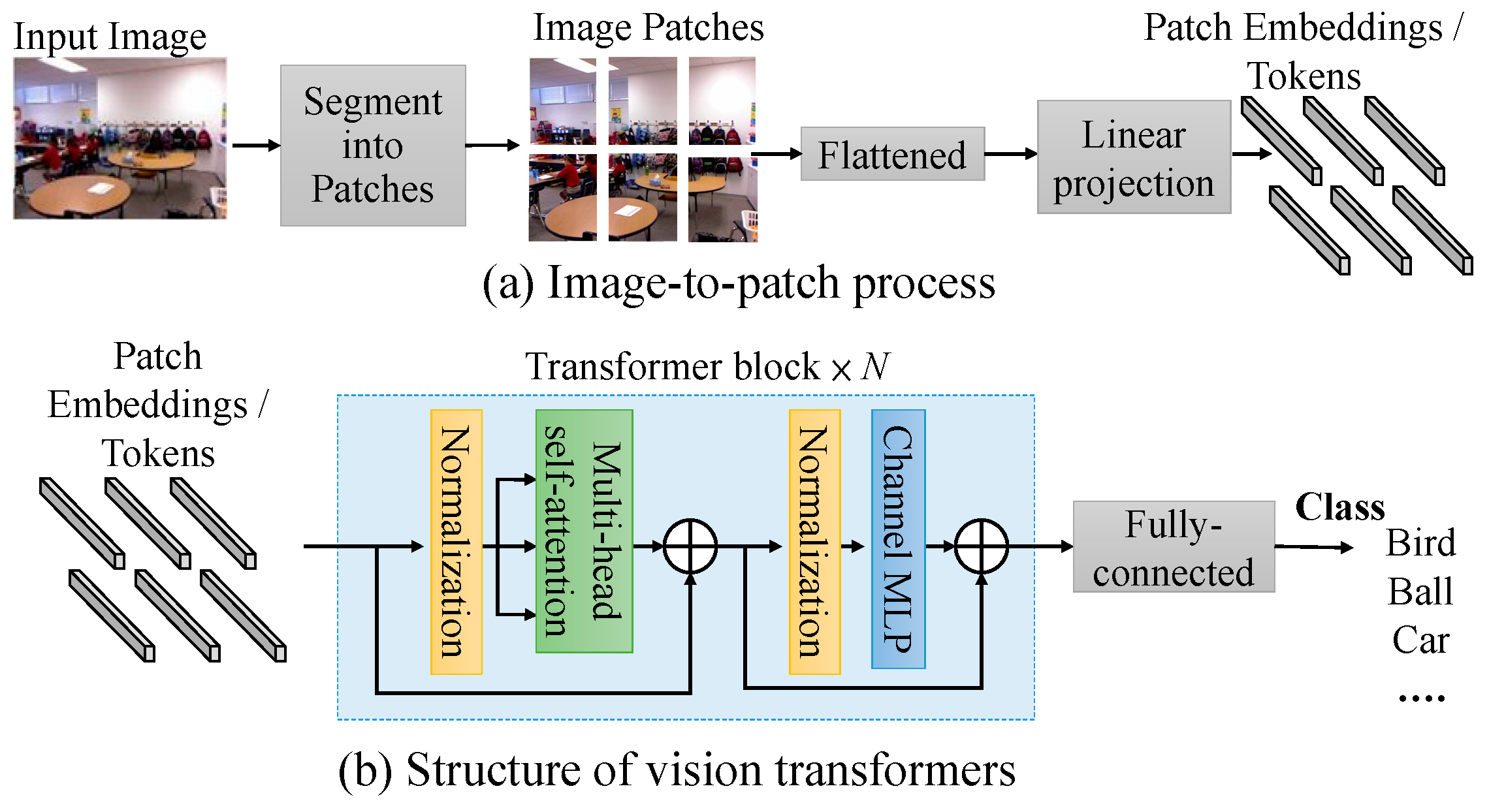
Figure 2.
Architecture of Atrous spatial pyramid pooling.
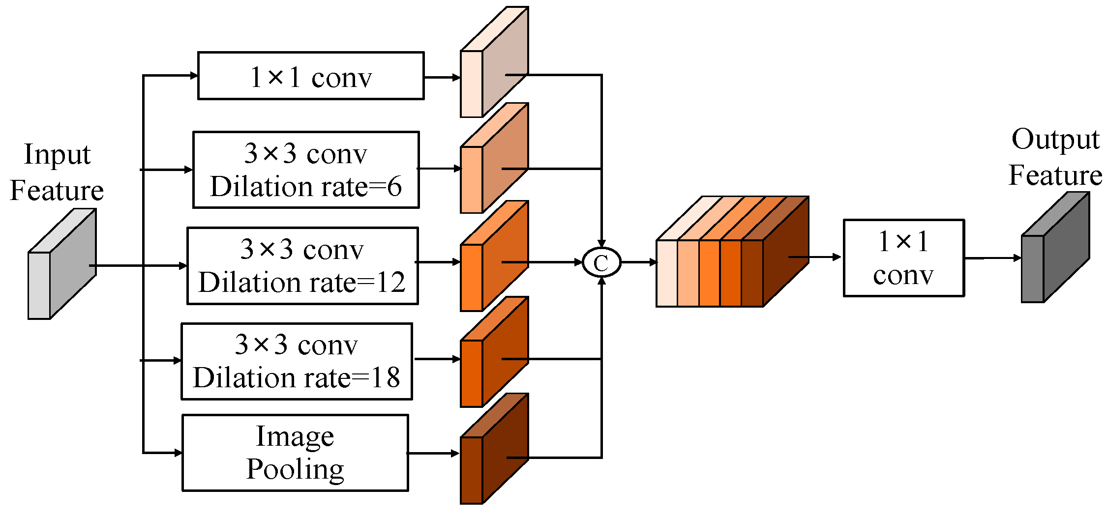
Figure 3.
Structure of selective feature fusion (SFF) module [16].
Figure 3.
Structure of selective feature fusion (SFF) module [16].
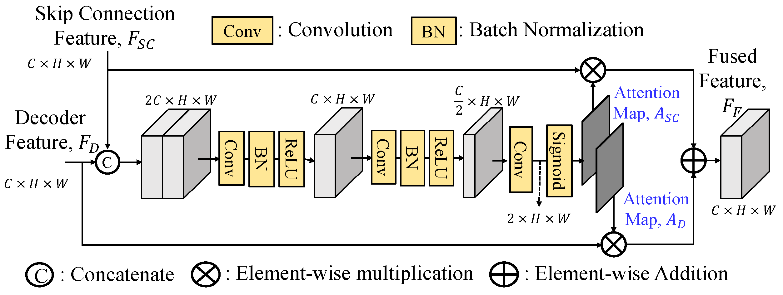
Figure 4.
Basic framework of the proposed RVTAF depth estimation network.
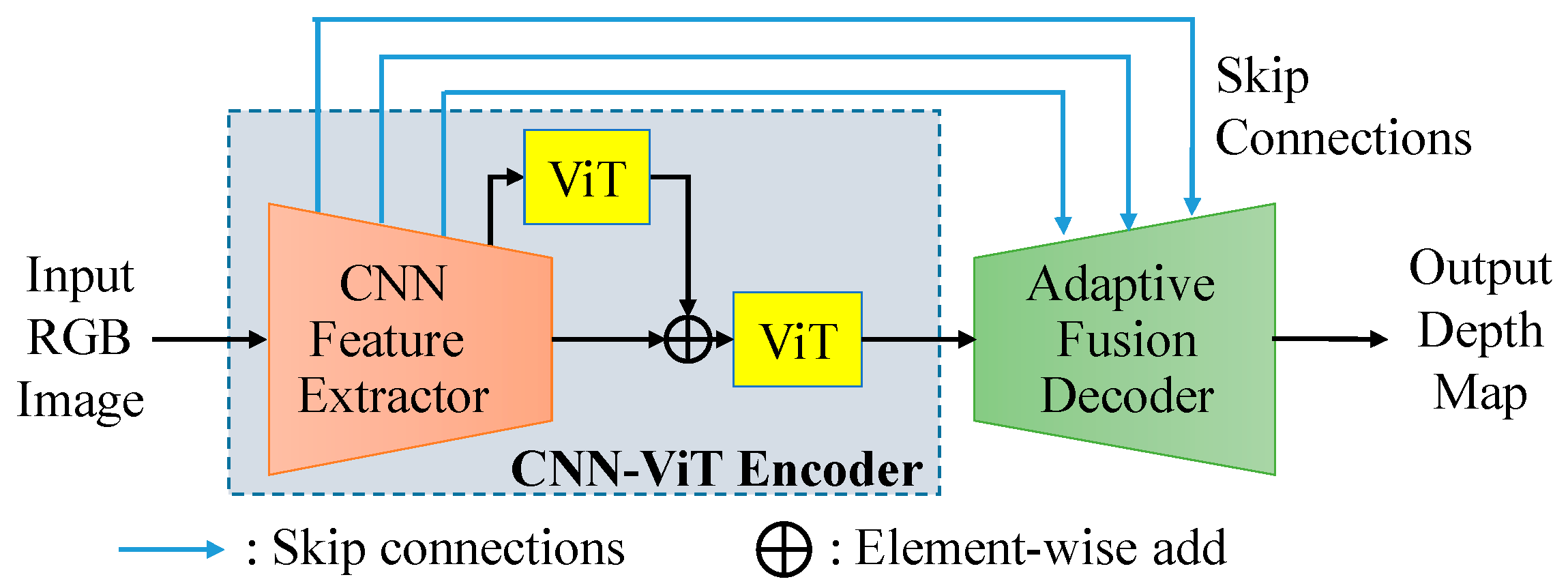
Figure 5.
Detailed structure of the final CNN-ViT encoder.
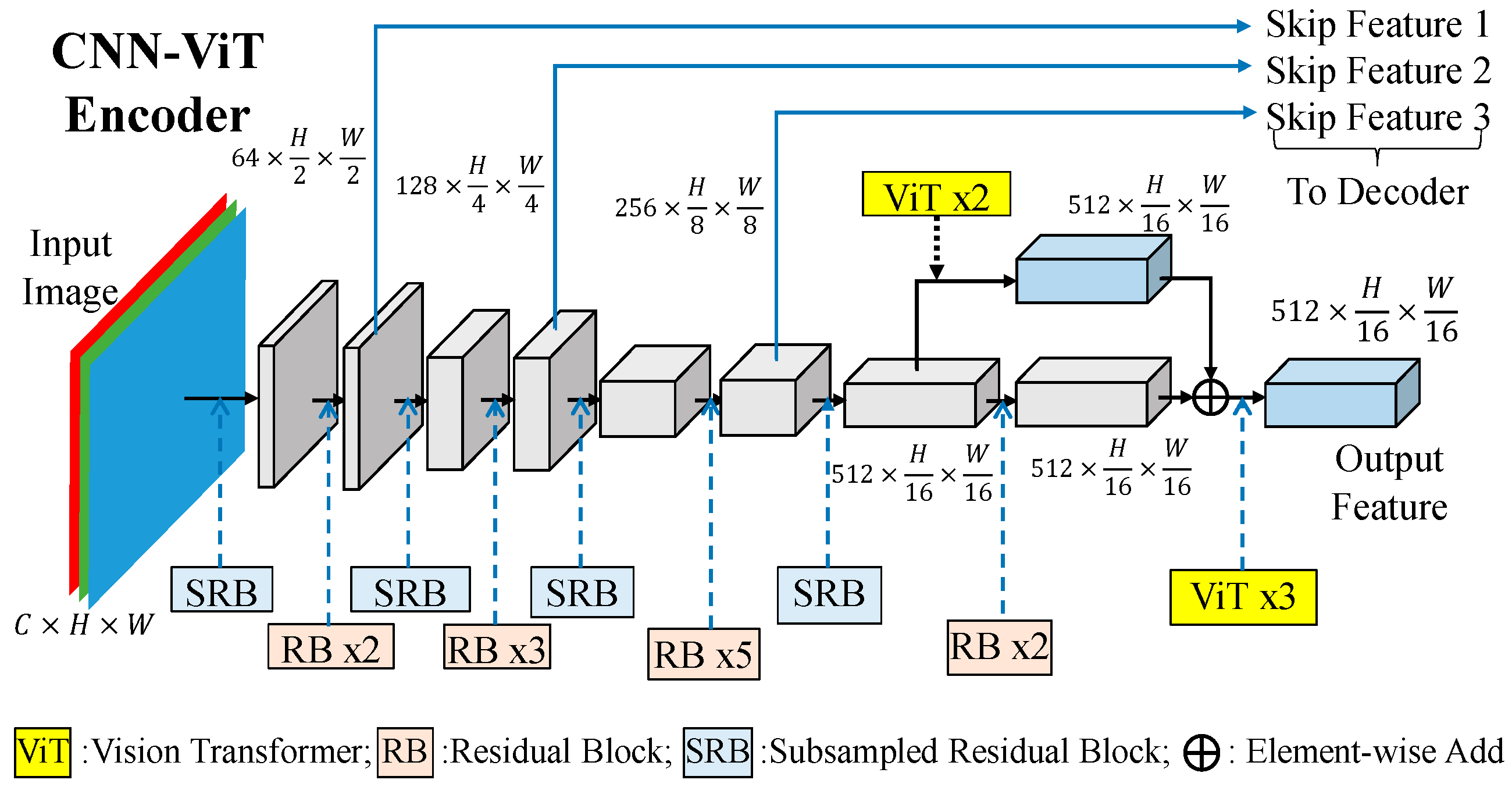
Figure 6.
The structure of subsampled residual block (SRB).
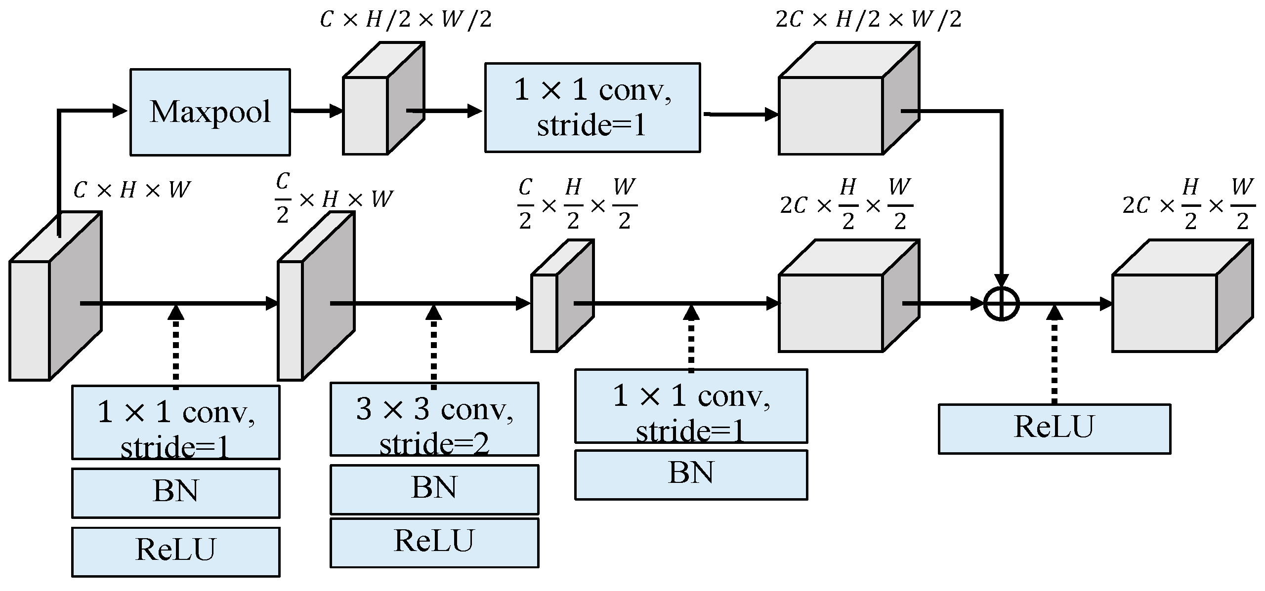
Figure 7.
The structure of residual block (RB).
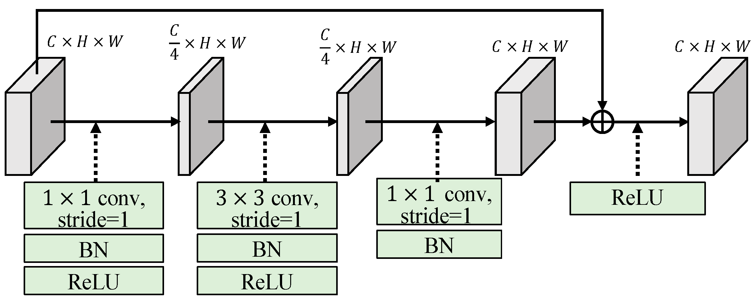
Figure 10.
The depicted positions for inserting the vision transformers.
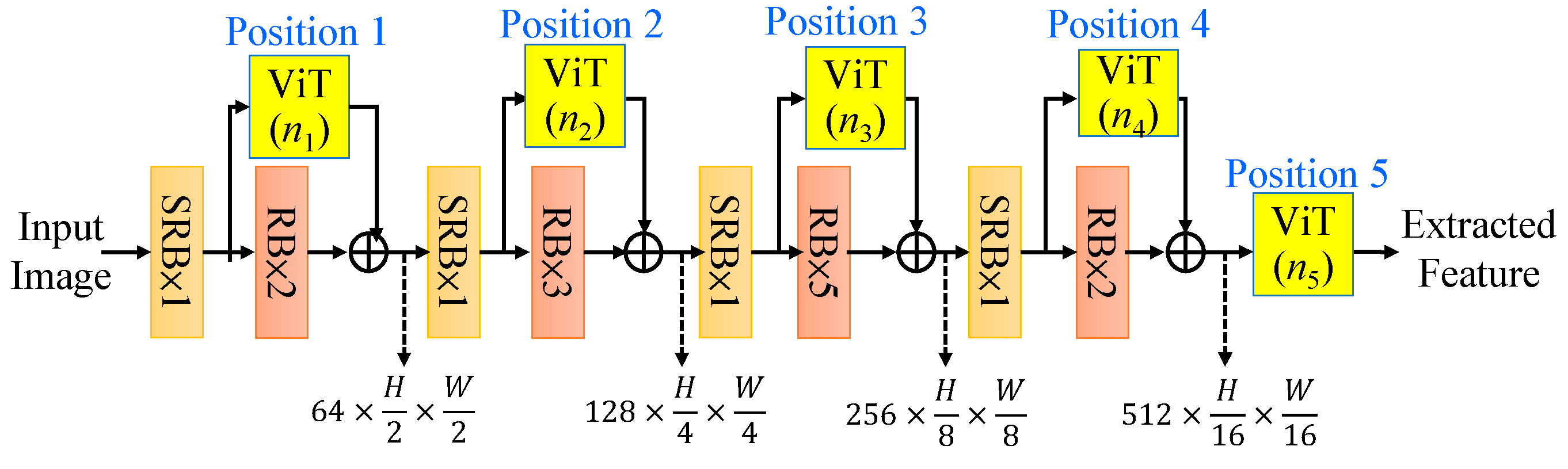
Figure 11.
The structure of the proposed adaptive fusion decoder in the proposed RVTAF depth estimation network.
Figure 11.
The structure of the proposed adaptive fusion decoder in the proposed RVTAF depth estimation network.
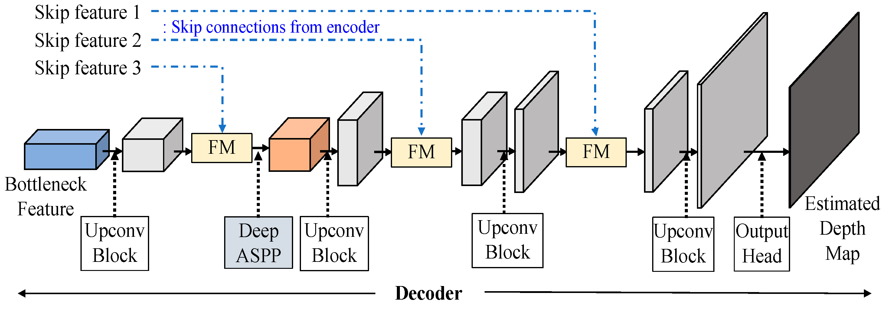
Figure 12.
Structure of separate enhancement addition fusion module (SEAFM).
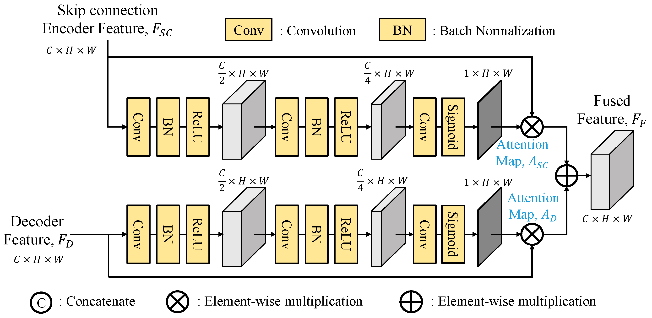
Figure 13.
Architecture of separate enhancement concatenation fusion module (SECFM).
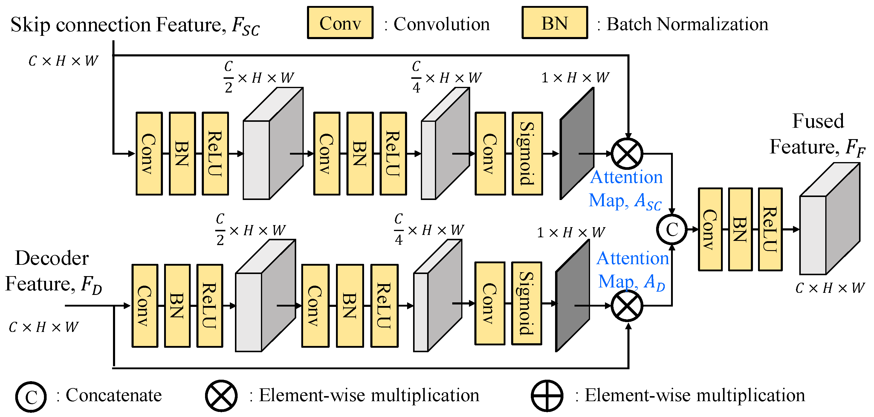
Figure 14.
Architecture of adaptive fusion module (AFM).
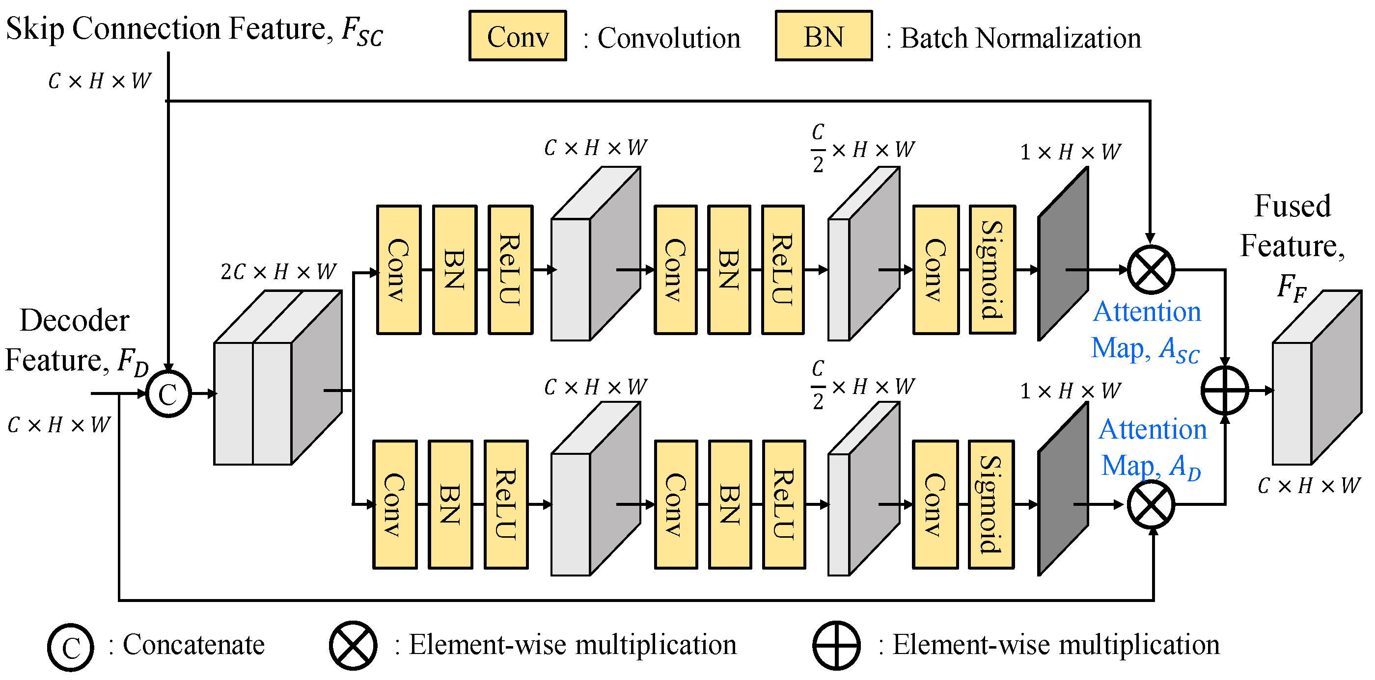
Figure 15.
Architecture of up-convolution block.
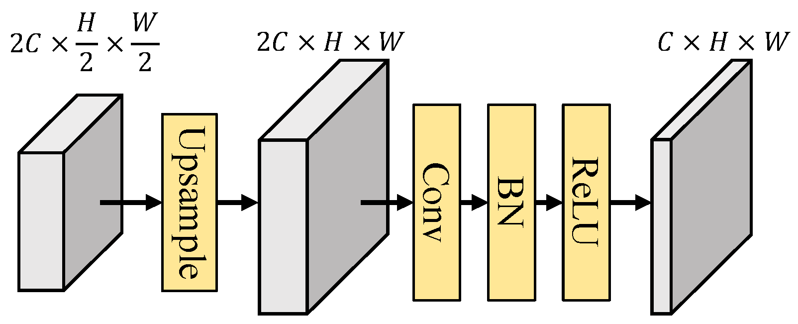
Figure 16.
The architecture of the Deep ASPP.
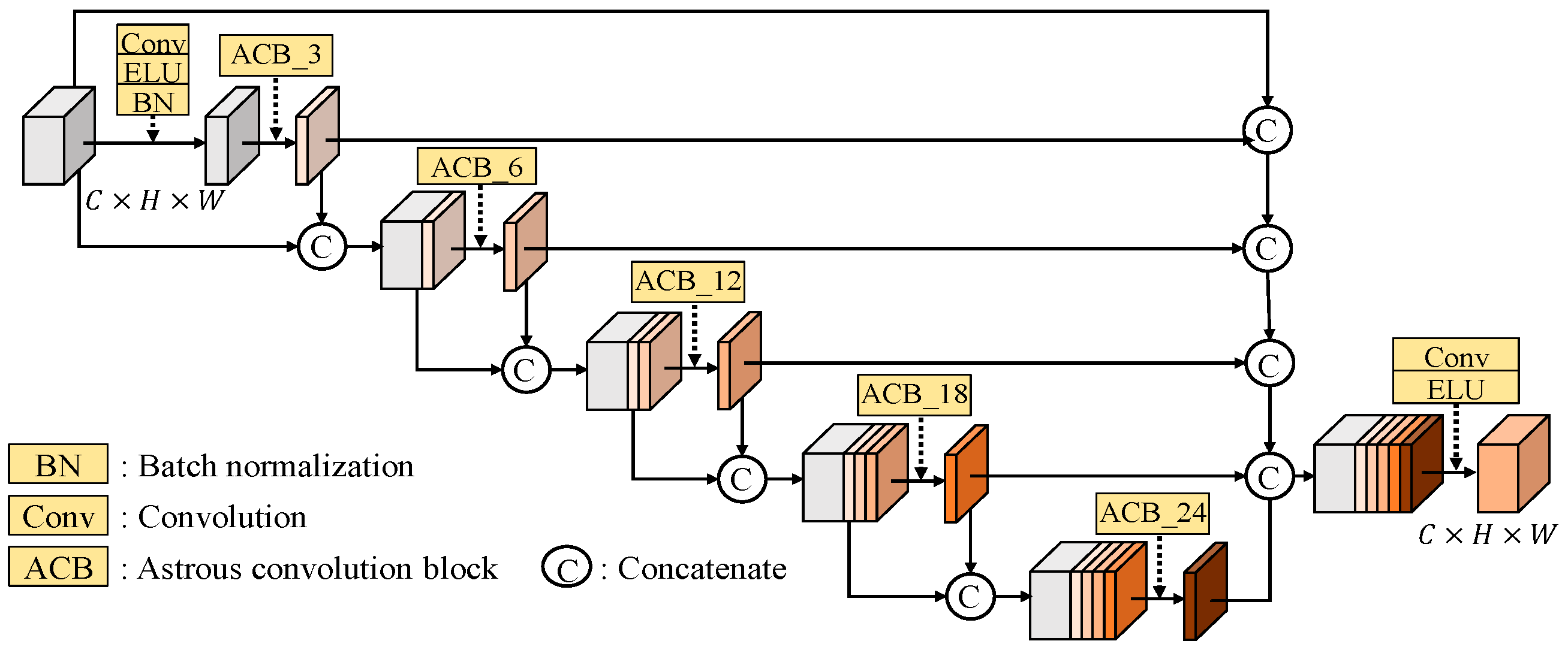
Figure 17.
Two seleced RGB color images and their corresponding depth maps in the NYU Depth V2 dataset.
Figure 17.
Two seleced RGB color images and their corresponding depth maps in the NYU Depth V2 dataset.
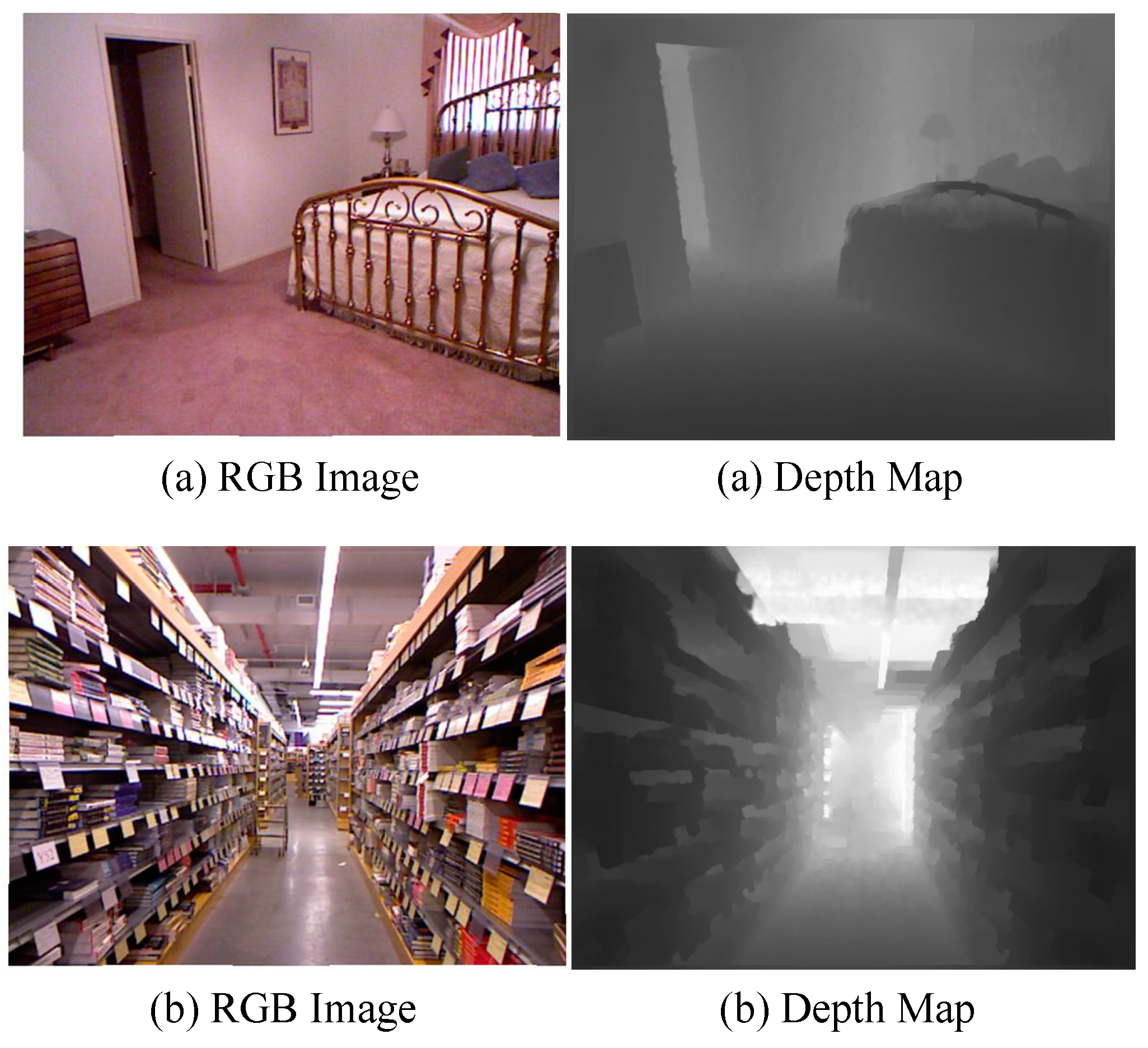
Figure 18.
Two selected RGB color images and their corresponding depth maps in the KITTI dataset.
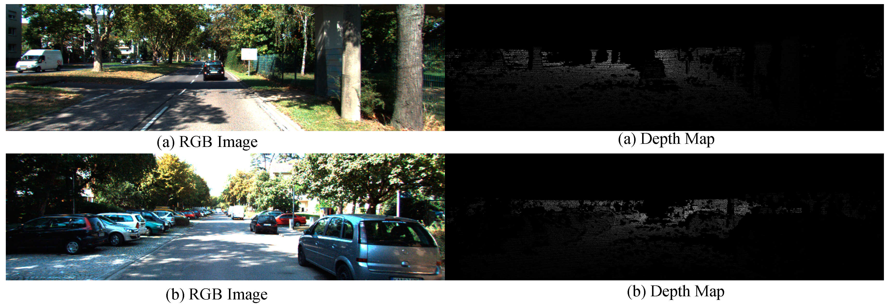
Figure 20.
Two selected images and their corresponding goundtruth depth maps on the NYU Depth V2 dataset.
Figure 20.
Two selected images and their corresponding goundtruth depth maps on the NYU Depth V2 dataset.
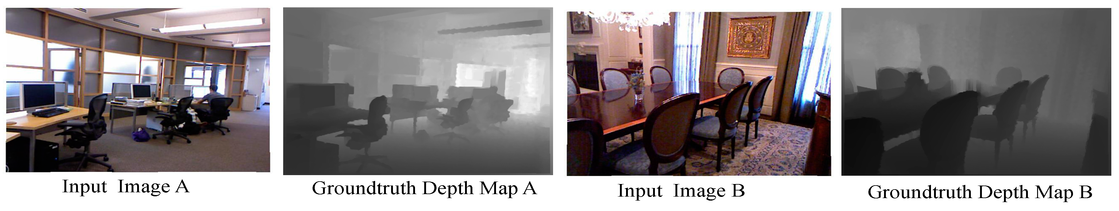
Figure 21.
Visualizations of depth estimation results obtained with the proposed RVTAF network and the existing approaches.
Figure 21.
Visualizations of depth estimation results obtained with the proposed RVTAF network and the existing approaches.
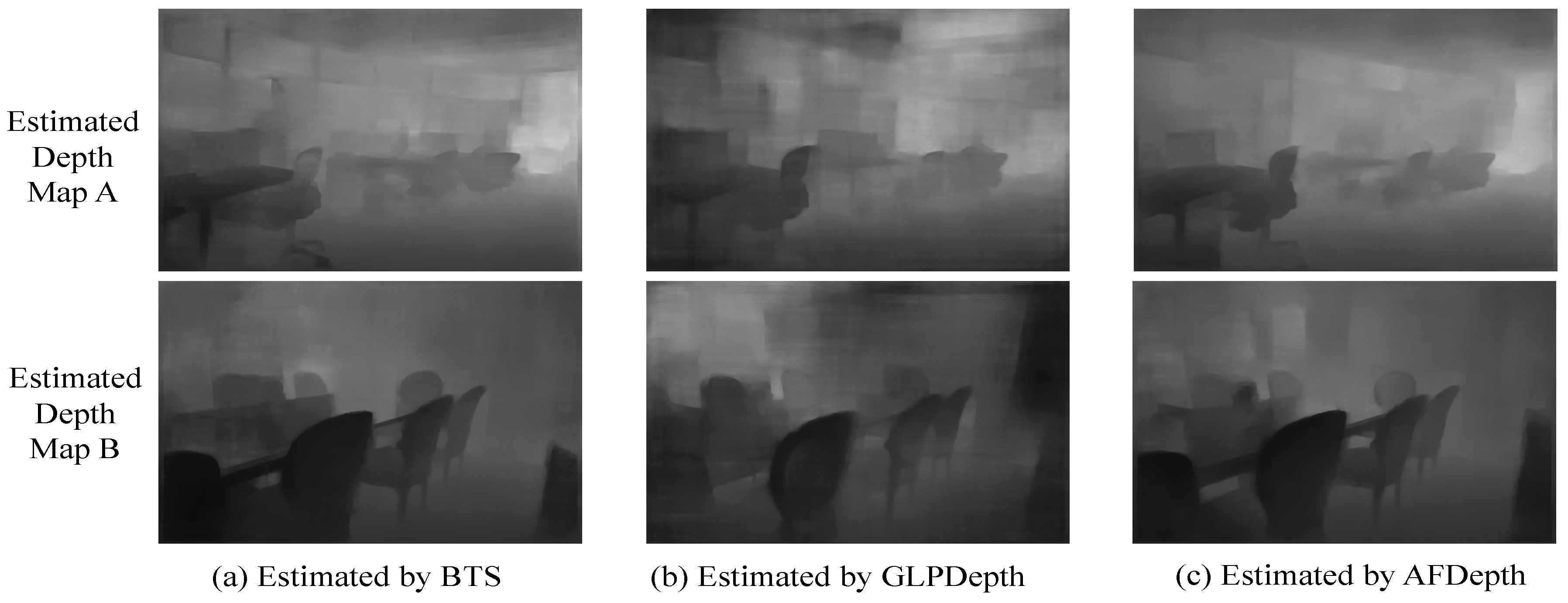
Figure 22.
Visualization comparisons of the depth estimation achieved by the proposed RVTAF depth estimation network and the existing approaches on the KITTI dataset.
Figure 22.
Visualization comparisons of the depth estimation achieved by the proposed RVTAF depth estimation network and the existing approaches on the KITTI dataset.
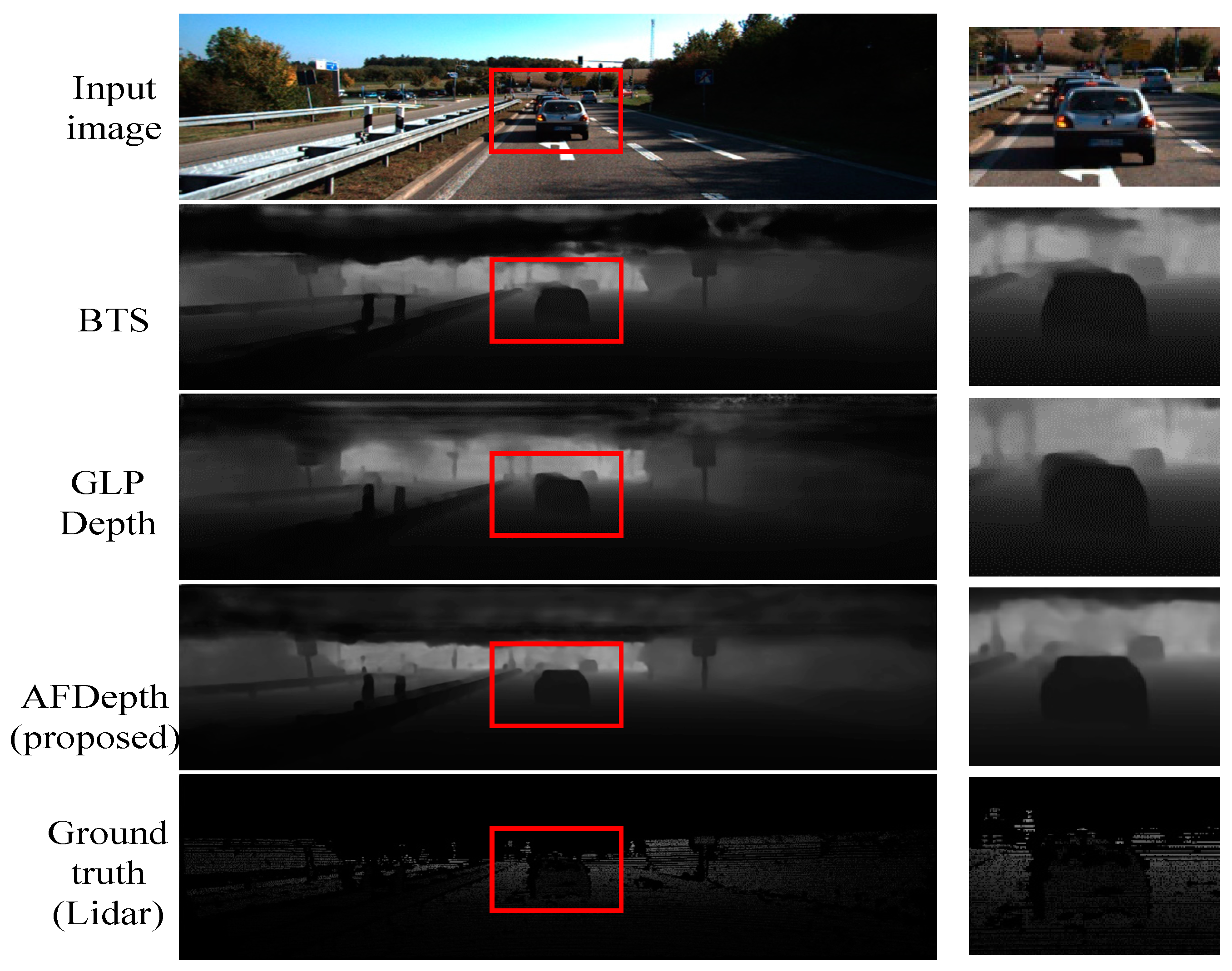

Table 1.
Experiments of various arrangements of ViTs evaluated on NYU V2 dataset Test 1449.
| ViT Positions n1 n2 n3 n4 n5 |
Flops (G) |
Params (MB) |
δ1↑ | δ2↑ | δ3↑ | RMS↓ | AbsRel↓ |
|---|---|---|---|---|---|---|---|
| 00000 (no ViTs) | 6.367 | 1.696 | 0.622 | 0.881 | 0.966 | 0.453 | 0.225 |
| 00005 | 13.229 | 64.815 | 0.875 | 0.967 | 0.991 | 0.371 | 0.105 |
| 00014 | 13.522 | 89.828 | 0.879 | 0.968 | 0.991 | 0.366 | 0.106 |
| 00023 | 13.522 | 89.828 | 0.880 | 0.971 | 0.992 | 0.360 | 0.101 |
| 00032 | 13.522 | 89.828 | 0.881 | 0.969 | 0.991 | 0.360 | 0.102 |
| 00041 | 13.522 | 89.828 | 0.878 | 0.969 | 0.992 | 0.365 | 0.102 |
| 00113 | 14.357 | 102.33 | 0.879 | 0.968 | 0.991 | 0.365 | 0.106 |
| 00122 | 14.357 | 102.33 | 0.881 | 0.968 | 0.990 | 0.361 | 0.105 |
| 00131 | 14.357 | 102.33 | 0.876 | 0.968 | 0.990 | 0.370 | 0.109 |
| 00212 | 14.603 | 102.33 | 0.878 | 0.969 | 0.991 | 0.363 | 0.101 |
| 00221 | 14.603 | 102.33 | 0.880 | 0.968 | 0.991 | 0.362 | 0.103 |
| 00311 | 14.849 | 102.33 | 0.879 | 0.970 | 0.992 | 0.363 | 0.104 |
| 01112 | 16.797 | 108.62 | 0.878 | 0.968 | 0.991 | 0.361 | 0.103 |
| 01121 | 16.797 | 108.62 | 0.882 | 0.970 | 0.992 | 0.357 | 0.100 |
| 01211 | 17.043 | 108.62 | 0.874 | 0.967 | 0.990 | 0.364 | 0.104 |
| 02111 | 18.030 | 108.62 | 0.880 | 0.968 | 0.991 | 0.358 | 0.105 |
| 11111 | 24.317 | 112.31 | 0.878 | 0.967 | 0.991 | 0.364 | 0.103 |
Table 2.
Experimental results with variations of fusion modules on NYU V2 testset 654.
| Fusion Modules |
Params (MB) | δ1↑ | δ2↑ | δ3↑ | RMS↓ | AbsRel↓ |
|---|---|---|---|---|---|---|
| SFF (baseline) | 1.665 | 0.696 | 0.907 | 0.971 | 0.651 | 0.206 |
| SEAFM | 0.836 | 0.718 | 0.919 | 0.975 | 0.615 | 0.192 |
| SECFM | 2.159 | 0.717 | 0.917 | 0.973 | 0.626 | 0.195 |
| AFM | 3.320 | 0.747 | 0.930 | 0.978 | 0.589 | 0.181 |
Table 3.
Comparison with existing approaches on NYU Depth V2 testset 654.
| Network | δ1↑ | δ2↑ | δ3↑ | RMS↓ | AbsRel↓ |
|---|---|---|---|---|---|
| BTS [26] | 0.762 | 0.940 | 0.984 | 0.565 | 0.167 |
| GLPDepth [16] | 0.605 | 0.872 | 0.962 | 0.769 | 0.235 |
| RVTAF Net* | 0.773 | 0.942 | 0.984 | 0.560 | 0.162 |
Table 5.
Comparisons the proposed RVTAF depth network and the existing approaches on KITTI dataset Eigen split.
Disclaimer/Publisher’s Note: The statements, opinions and data contained in all publications are solely those of the individual author(s) and contributor(s) and not of MDPI and/or the editor(s). MDPI and/or the editor(s) disclaim responsibility for any injury to people or property resulting from any ideas, methods, instructions or products referred to in the content. |
© 2024 by the authors. Licensee MDPI, Basel, Switzerland. This article is an open access article distributed under the terms and conditions of the Creative Commons Attribution (CC BY) license (http://creativecommons.org/licenses/by/4.0/).
Copyright: This open access article is published under a Creative Commons CC BY 4.0 license, which permit the free download, distribution, and reuse, provided that the author and preprint are cited in any reuse.


