
Submitted:
17 November 2024
Posted:
19 November 2024
You are already at the latest version
Abstract
The NIEP (National Institute of Earth Physics) monitors and analyzes seismicity in Romania. Over time, the monitoring stations equipped with seismic equipment have become multifunctional with new devices for measuring gas emissions, the magnetic field, the telluric field, solar radiation, etc. This made it possible to introduce a seismic forecasting system, which is intended to extend the alert time of the warning system based solely on seismic data. The realization of an OEF (Operational Earthquake Forecasting) aims to extend the warning time from 25-30 seconds before an earthquake manifests its effects with a magnitude of more than 4.8R to several hours or even days. The AFROS project (PCE119/4.01.2021) introduced fundamental research studies in the development of the OEF system. The results are now public in the form of real-time analysis of radon and CO2 emissions on the page http://afros.infp.ro/AFROS.php?link=dategeofizice. The monitored area is Vrancea because it generates the most destructive earthquakes in Romania, with effects in neighboring countries (Bulgaria, Ukraine, and Moldova). The structure of the monitoring network and the methods used can be adapted to other seismic zones depending on their particularities. The data acquisition includes analog signals (e.g., magnetic field, well temperature), digital data (e.g., radon, CO2, well water level), and from other sources (e.g., VLF receivers, Kp geomagnetic factor from NOAA). All data ends up in a database that can be accessed through an API and the result will be in JSON format (https://data.mendeley.com/datasets/28kv3gsgcz/2). The methods used include the detection of events by exceeding certain thresholds, STA/LTA type data analysis, and analysis of seismic bulletins (parameters a, b from the Gutenberg Richter law). In each case, the application of these methods involves particularities that make the monitoring network a novelty in activities of this type. The experimental results indicate the possibility of using the parameter b from the Gutenberg Richter law and the emission of gases in the real-time seismic forecast. This was known from previous analyses carried out on data series on the periods in which earthquakes with a magnitude greater than 4.5R occurred. The novelty is that currently this is done continuously and the results are public.
Keywords:
OEF (Operational Earthquake Forecasting)
; multidisciplinary monitoring network
; seismic pre-cursor phenomena
; radon
; CO2 emission
1. Introduction
This article presents the evolution of the seismic forecasting system the OEF of NIEP. Its theoretical approaches began several years ago, but its development depended on funding sources. The last important project was AFROS (Analysis and Forecasting of Romanian Seismicity, 2021 - 2023) based on fundamental research (http://afros.infp.ro/proiect_en.php). We went through a year of checking the Vrancea seismicity assessment methods and the real-time monitoring network. Previous articles have described the structure and evolution of the data network, including the type of equipment [1,2,3,4]. We expanded the monitoring area, number, and type of equipment with applications in the field of climate effects. The main goal of creating an automated seismic forecasting system (OEF) was partially achieved because the detection algorithms were not fully implemented and not all seismic precursors were used. In the article, we will present the way of implementation, and the results obtained, and we will compare the detection methods used. In many cases, OEF systems are based only on the current earthquake activity and use the ETAS, ETES, STEP, Omori–Utsu, and Gutenberg–Richter laws as basic models (e.g. [5,6,7]). These methods have not been verified for our area of interest, Vrancea. It is characterized by crustal and intermediate earthquakes and there are not necessarily aftershocks after a main shock. A particularity that is confirmed for the Vrancea area is the decrease in the value of the "b" parameter from the Gutenberg-Richter law (GR_b) for more than 18 days [5] before the occurrence of an earthquake with a greater magnitude than 5R. In this case, we use the seismic bulletins that NIEP produces after each earthquake and to which we have access before they are public. These are retrieved by the ISC after review, but not in real-time. The analysis of the 'b' parameter using data from seismic catalogs shows that its variation depends on the specifics of the analyzed area [8]. The b-values in New Zealand initially increase and then return to normal [9], unlike Vrancea which decreases and returns to normal after the earthquake. A complete OEF also includes precursor parameters (radon in the air, water, soil, CO2, electromagnetic field, thermal anomalies in the soil, water, acoustic noise, infrasound, soil deformation, etc.). In [10], multidisciplinary monitoring networks in China, Greece, Italy, Japan, Russia, and the USA are described as part of an OEF structure for short-term earthquake forecasting. An important problem highlighted in the article is how information is communicated by scientists to the public in order not to cause confusion and panic. For this reason, the operational forecast of earthquakes is not made public, and many results are presented only in scientific papers. For this reason, we have limited ourselves to a concise presentation within the AFROS project platform where real-time information is presented regarding gas emissions (radon and CO2) correlated with seismicity (http://afros.infp.ro/AFROS.php?link=dategeofizice). The data we use are accessible on http://geobs.infp.ro through an API with a result in JSON format.
The project TURNkey (Towards more Earthquake-resilient Urban Societies through a Multi-sensor-based Information System enabling Earthquake Forecasting, Early Warning, and Rapid Response actions), grant agreement No 821046, includes an OEF system in addition to seismic methods. This complex project makes a cost-benefit analysis to assess the potential of an OEF system before a seismic event in Europe. The paper [11] assesses whether an evacuation of the population would have been cost–beneficial in cases of high seismic event probability. In our case, there are rules for the transmission of messages that could cause panic, as in the case of a strong earthquake in the Vrancea region. Similarly, the NIEP Rapid Earthquake Early Warning System (REWS) transmits information in real-time to specialized organizations for emergencies. Earthquake forecasts can also be transmitted via the same data channels. They are currently displayed in the form of a graphic on the AFROS website. The choice of the Vrancea area is optimal from a cost-benefit point of view, it is characterized by deep earthquakes that can reach a magnitude of 7.5R, the effects being devastating in large areas including Bucharest.
In this paper, we analyze two detection methods used in NIEP’s OEF. One is based on acquisition software that provides a triggering–detriggering facility. This method is used in all seismic digitizers. The second method is STA/ LTA (Short-Term Averages/ Long-Term Averages) detection algorithm type Allen [12,13,14] applied on signal integration and described in [1,2,3,4]. We followed the behavior of the detection algorithms for one year to go through the situations of seasonal variations in gas emissions (radon and CO2). The first method is based on the detection of events in the monitoring stations, which corresponds to a decentralized structure. This allows a local decision (activating an engine, opening a valve, etc.) useful in extreme situations where response time matters. The STA/LTA algorithm requires a large amount of data, which implies larger resources. In this case, a data server is necessary to analyze the information transmitted from the monitoring stations. The real-time solution implemented in the AFROS platform uses the trigger information from the multidisciplinary stations and a central server that gathers all the messages in a decision matrix that evaluates the possibility of producing a seismic event. The STA/LTA method is tested separately to evaluate if the results are closer to reality. The OEF structure must be flexible and allow the introduction of new algorithms that work in parallel. The first method based on the trigger in the stations is the simplest and easy to implement with low costs. At this moment the trigger thresholds are fixed with the possibility for an operator to modify them. They can be adaptive depending on the time or season because the gas emission is dependent on these factors. The data analysis shows a dependence of radon and CO2 depending on the temperature, which has unexpected variations under the conditions of climate change. In this case, the level trigger method is not the safest. Until now, the results of its application have been unexpectedly good for radon and CO2 monitored in the Vrancea area. The AFROS project (gttp://afros.infp.ro) presented many forecasting methods, but their real-time implementation requires additional resources.
2. New Equipment in the Multidisciplinary Monitoring Network
The multidisciplinary network was developed with new equipment for measuring radon, thoron, and CH4. They were installed in the Vrancea area as part of the OEF and will soon be operational (Table 1).
Two RTM 1688-2 equipment that measures radon (222Rn) and thoron (220Rn) are now in Vrancioaia and Plostina locations (Table 1, Table 2). The novelty is not only the thoron but also the alpha spectrum of radon. We have previous radon data at the 2 locations, but not as detailed. The equipment involves higher costs than the previous ones, and we must analyze whether the results are better. Both radon (222Rn) and thoron (220Rn) are seismic precursors [15,16].
Table 2 shows what data offered by RTM1688-2 and Table 3 shows the Radon Scout Plus used in the same location. One Radon Scout equipment is still in Plostina installed in a pit (Table 4).
The difference between the equipment used can be seen in Table 2, Table 3, and Table 4. Radon Scout has less memory than Radon Scout Plus, no atmospheric pressure, and older firmware. The RTM1688-2 is more efficient with an air pump but less reliable and noisy. Its use brings more information about radon, which allows the creation of an alpha spectrum and, in addition, thoron. In its case, we have two values for radon (‘Radon’ and ‘Radon* fast’), four regions of interes (ROI1 – ROI4), and 38 channels alpfa spectrum (Table 2). To better understand the functions of RTM16988-2, we refer to Figure 1 [17], where the radon decay chain appears. According to Manual_RTM1688-2_EN_24-01-2024 (SARAD), the alpha particles emitted by Polonium 218 are recorded in a semiconductor detector resulting in a number of ions proportional to the radon gas concentration. ‘RTM1688-2 offers two calculation modes for the Radon concentration, one (Slow) includes both, Po-218 and Po-214 decays and the other one includes Po-218 only (Fast). Each Po-218 decay causes one more detectable decay by the Po-214 which is delayed about 3 hours because of the superposed half-life times of those nuclides’, according to Manual_RTM1688-2_EN_24-01-2024 (SARAD). For this reason, we chose a time of 3 hours for the radon measurement which we redistribute to one minute for compatibility with the other data.
RTM1688-2 measures Thoron (220Rn), too. Figure 2 present the Thorium (232 Th) decay chain where 220Rn, 216Po, 212Bi, and 212Po apare. Both Figure 1 and Figure 2 are usefull to understand the measurements of RTM1688-2.
Figure 3, Figure 4 and Figure 5 and Figure 7, Figure 8, Figure 9, Figure 10 and Figure 11 are the results of using Radon Vision (SARAD) software. The earthquake with magnitude 5.4R is our case study and is marked in the figures.
Figure 3 and Figure 4, which show radon*(fast) and radon in the same location and time interval, it follows that there are no big differences between the two quantities. The Alpha Spectrum diagram for the Plostina site (Figure 5, the same time interval) includes information from Figure 1 and Figure 2. The determination of the Alpha Spectrum from RTM1688-2 data is possible with channels 1 – 38 from Table 2 (representation in Figure 6). The same graphics are for the Vrancioaia location (Figure 7, Figure 8, Figure 9). And in this case, there are no big differences between radon*fast and radon.
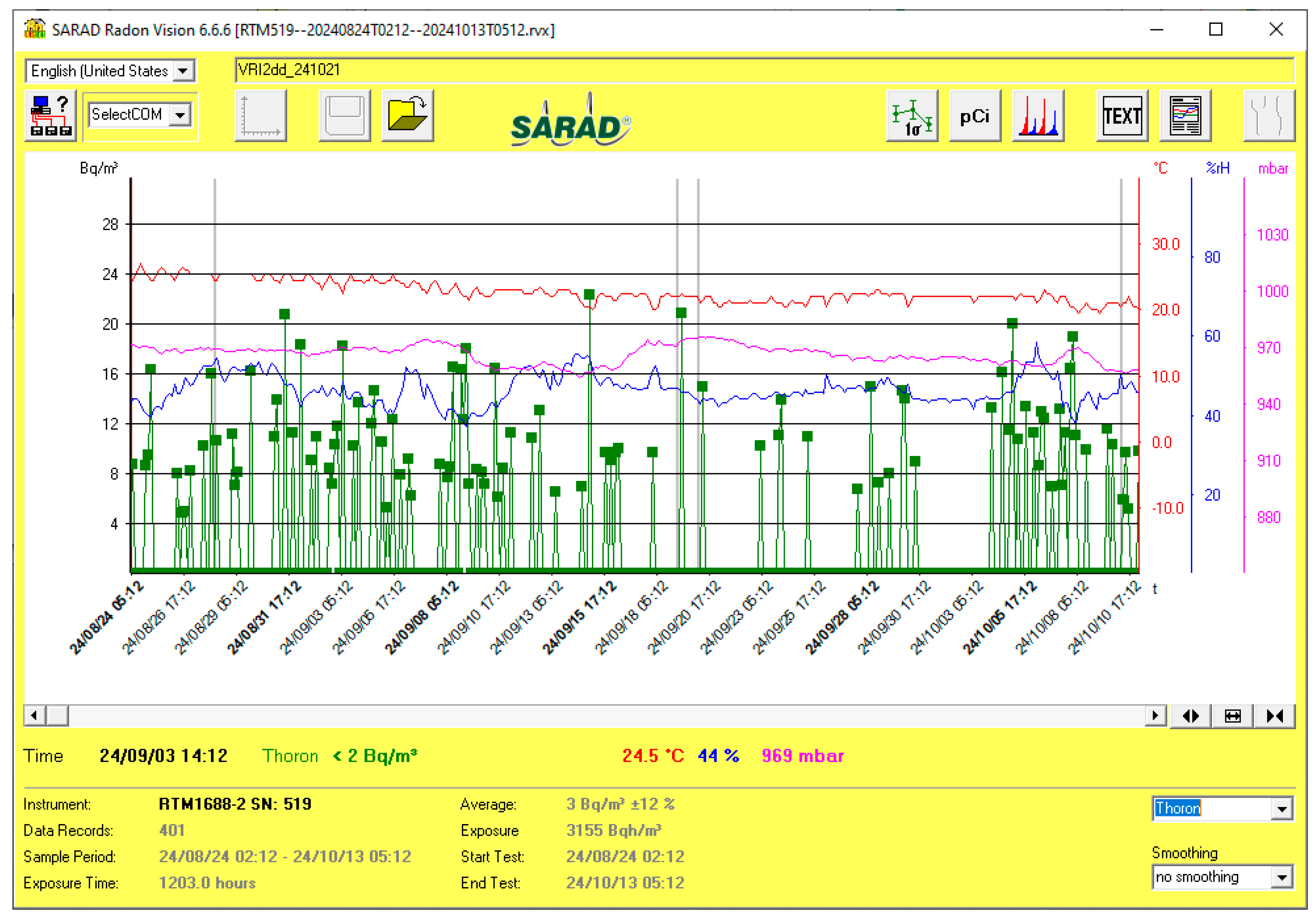
Thoron is presented with the same Raon Vision software in Figure 10 and Figure 11. On the same graphs, there are represented temperature, humidity, and atmospheric pressure.
Figure 3.
Radon* (fast) evolution in Plostina site, RTM1688 data (Radon Vision software).
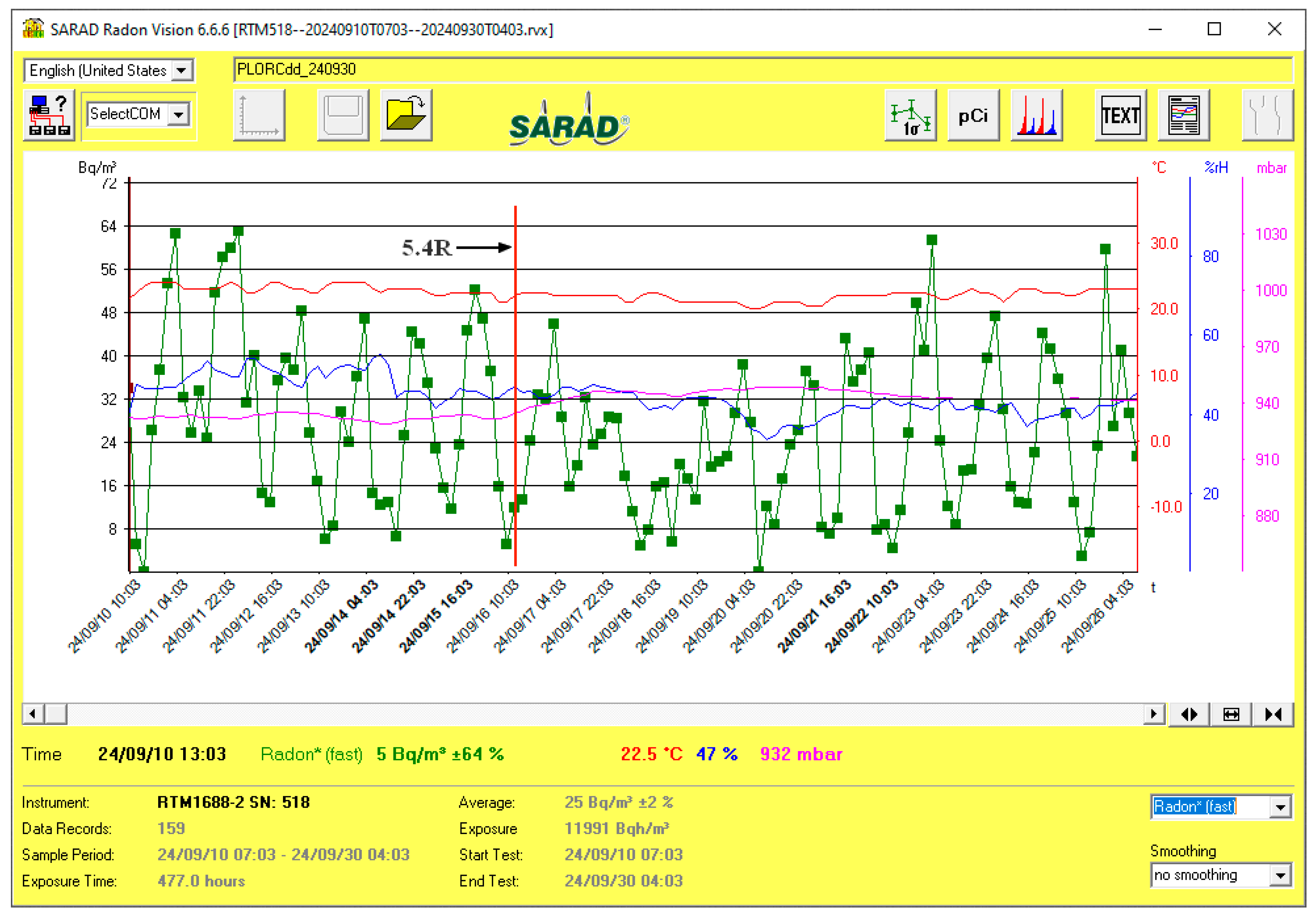
Figure 4.
Radon in Plostina location, RTM1688 data (Radon Vision software).
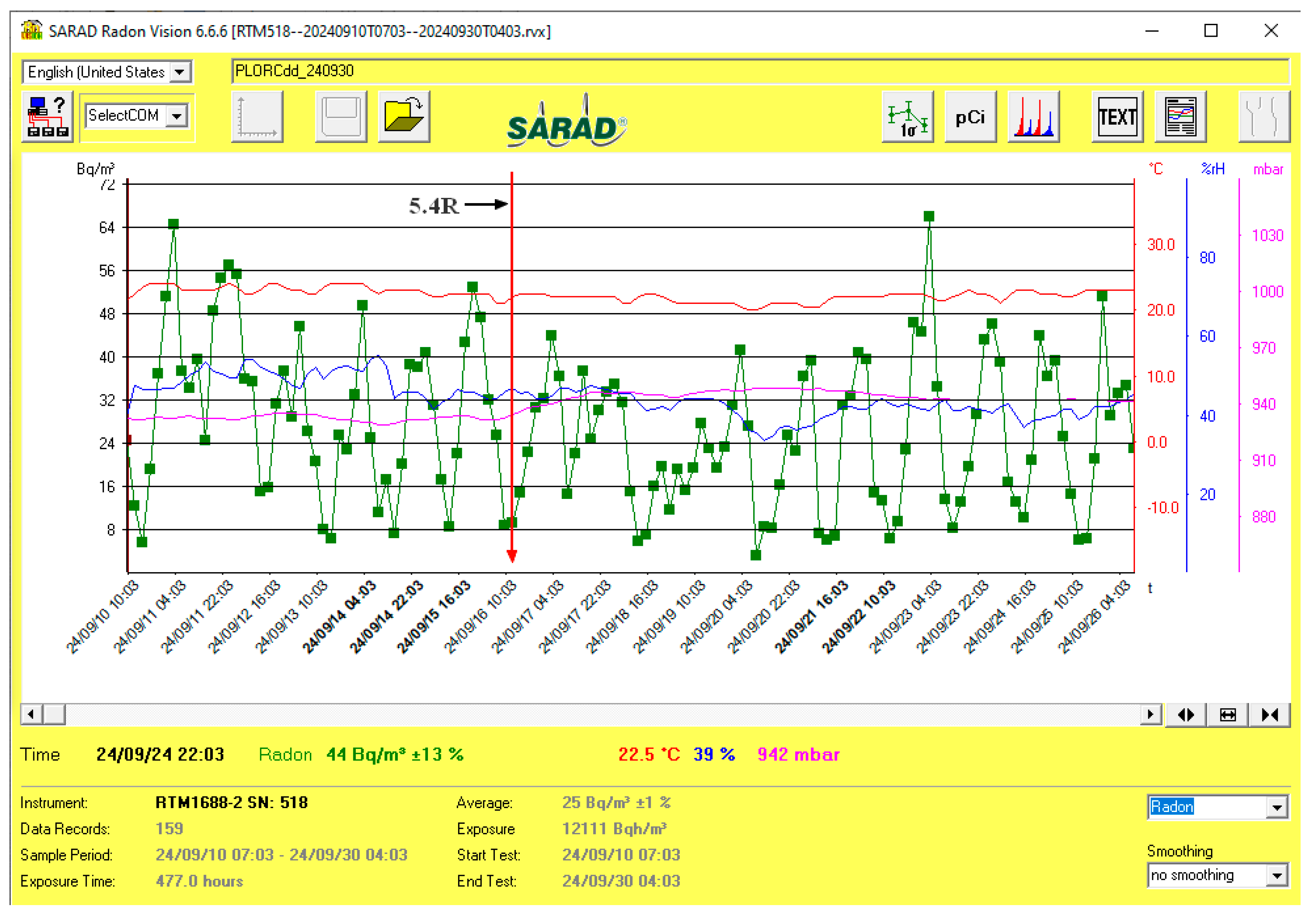
Figure 5.
Alpha Spectrum diagram for Plostina site (Radon Vision software).
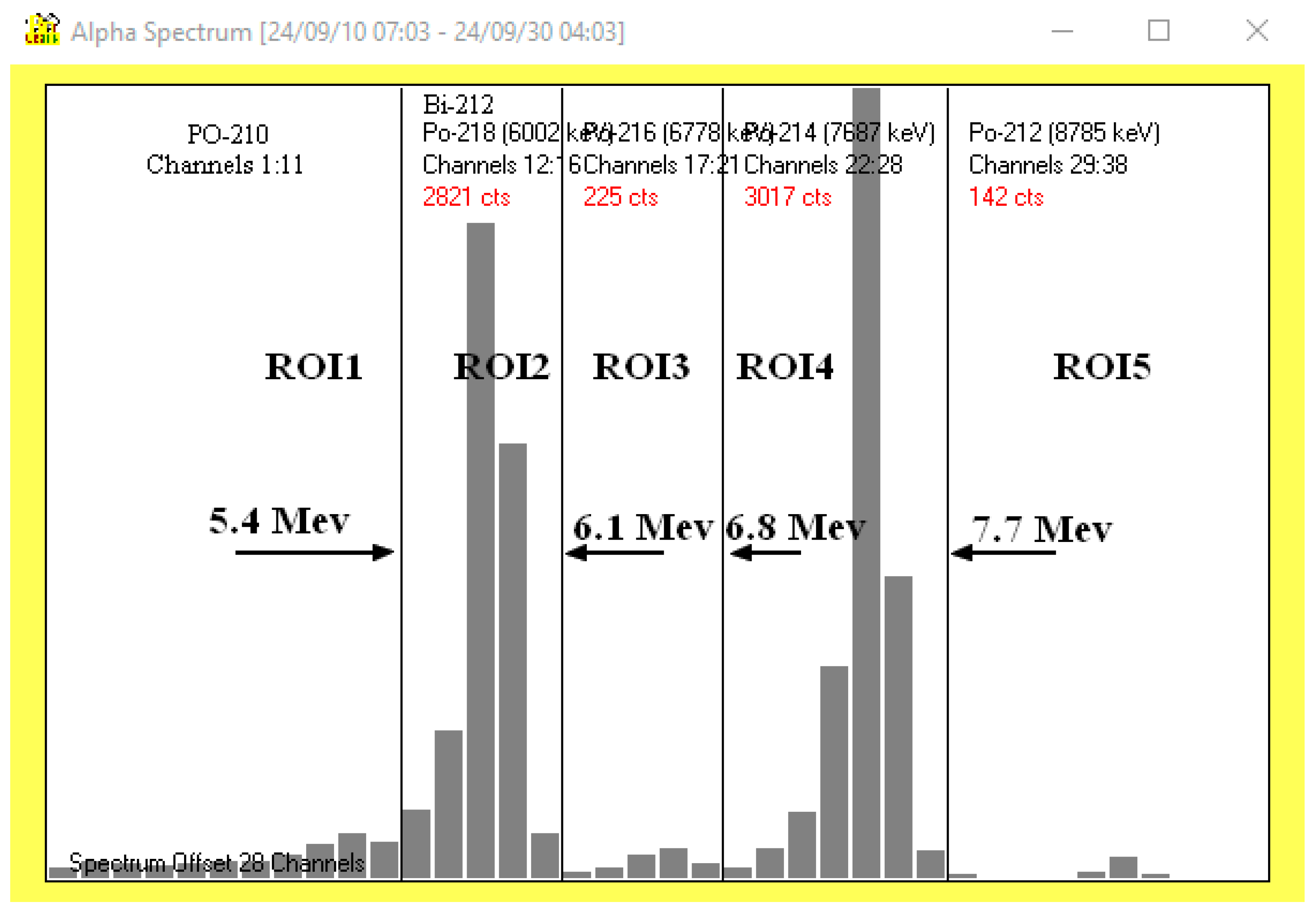
Figure 6.
Determination of the Alpha spectrum from RTM1688-2 data.
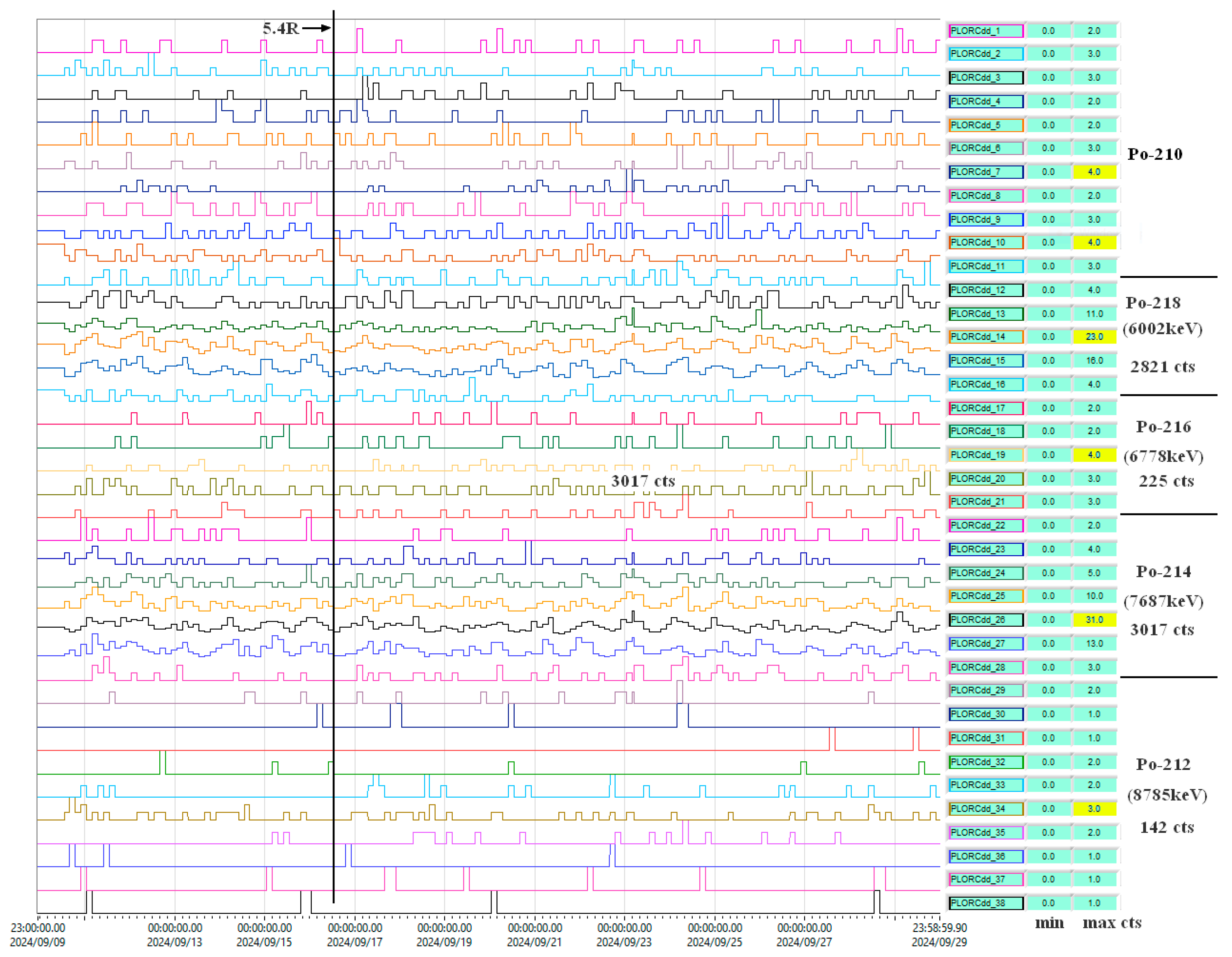
Figure 7.
Radon* (fast) evolution in Vrancioaia site, RTM1688 data (Radon Vision software).
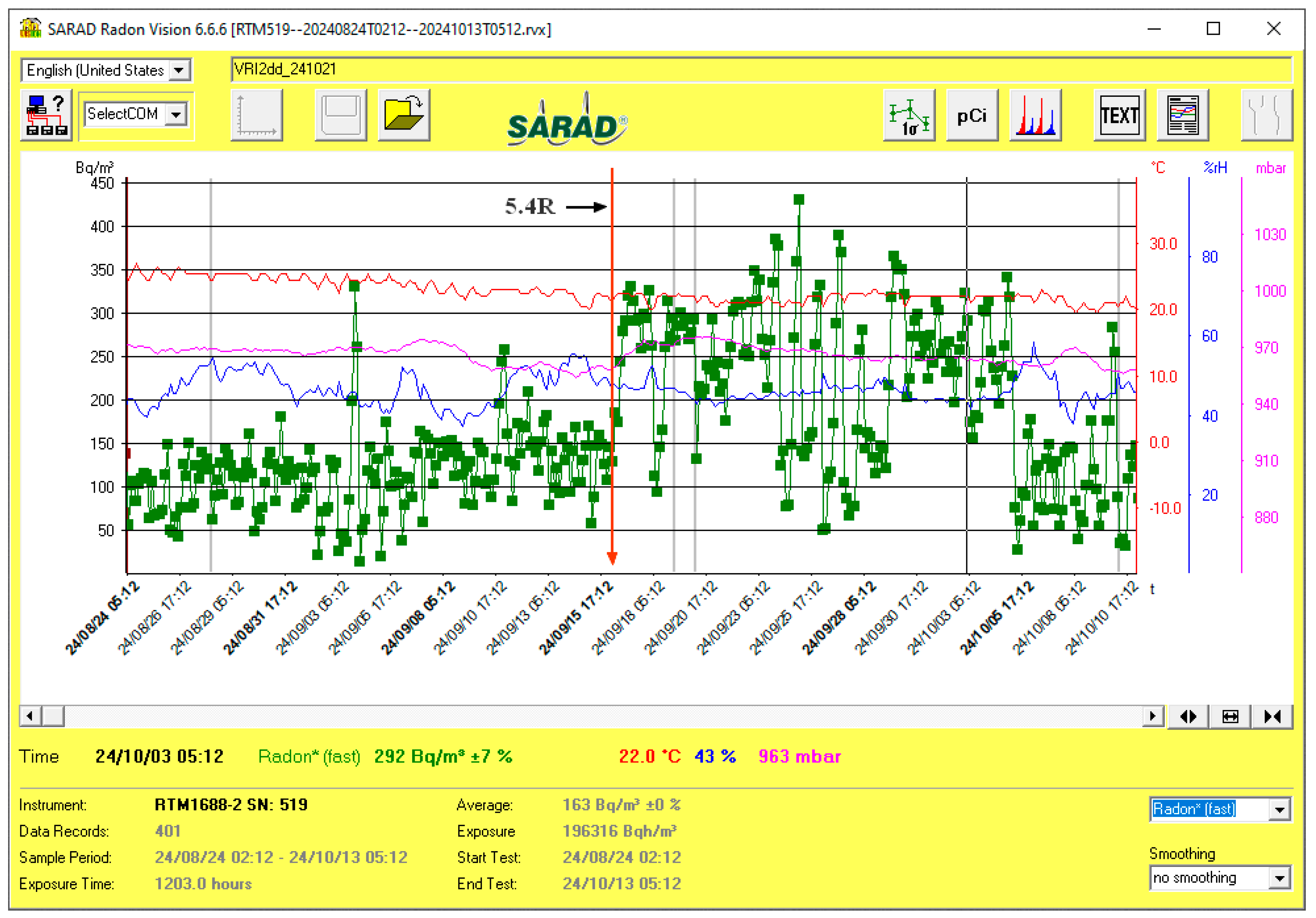
Figure 8.
Radon in Vrancioaia location, RTM1688 data (Radon Vision software).
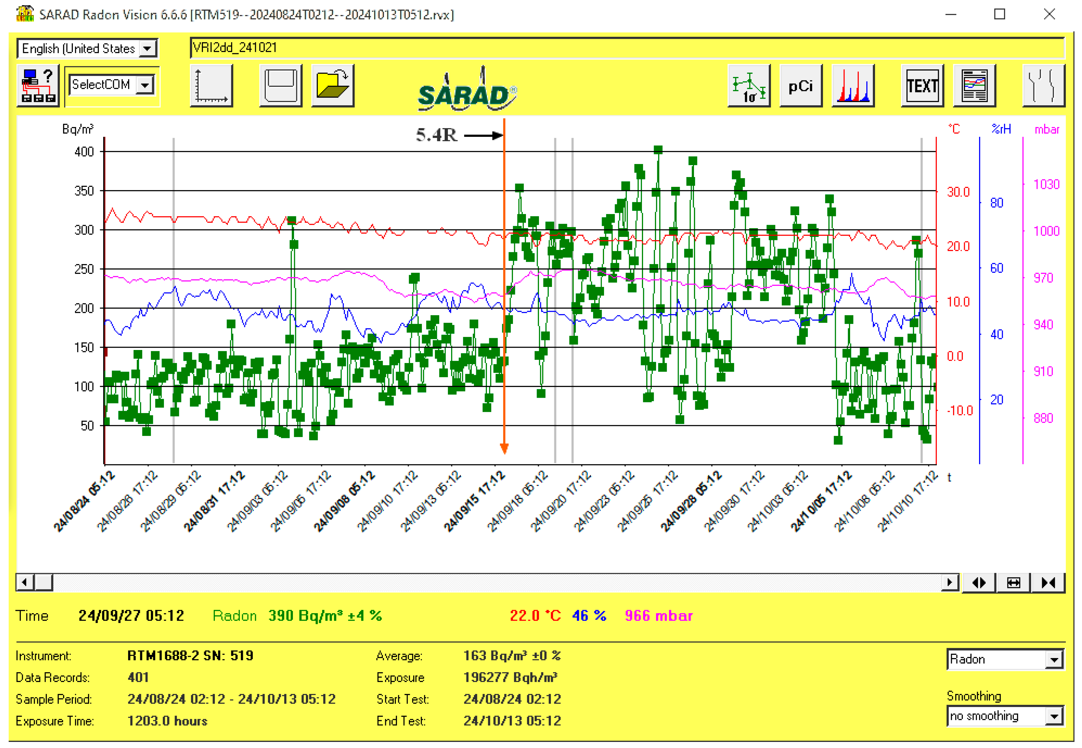
Figure 9.
Alpha Spectrum diagram for Vrancioaia location (Radon Vision software).
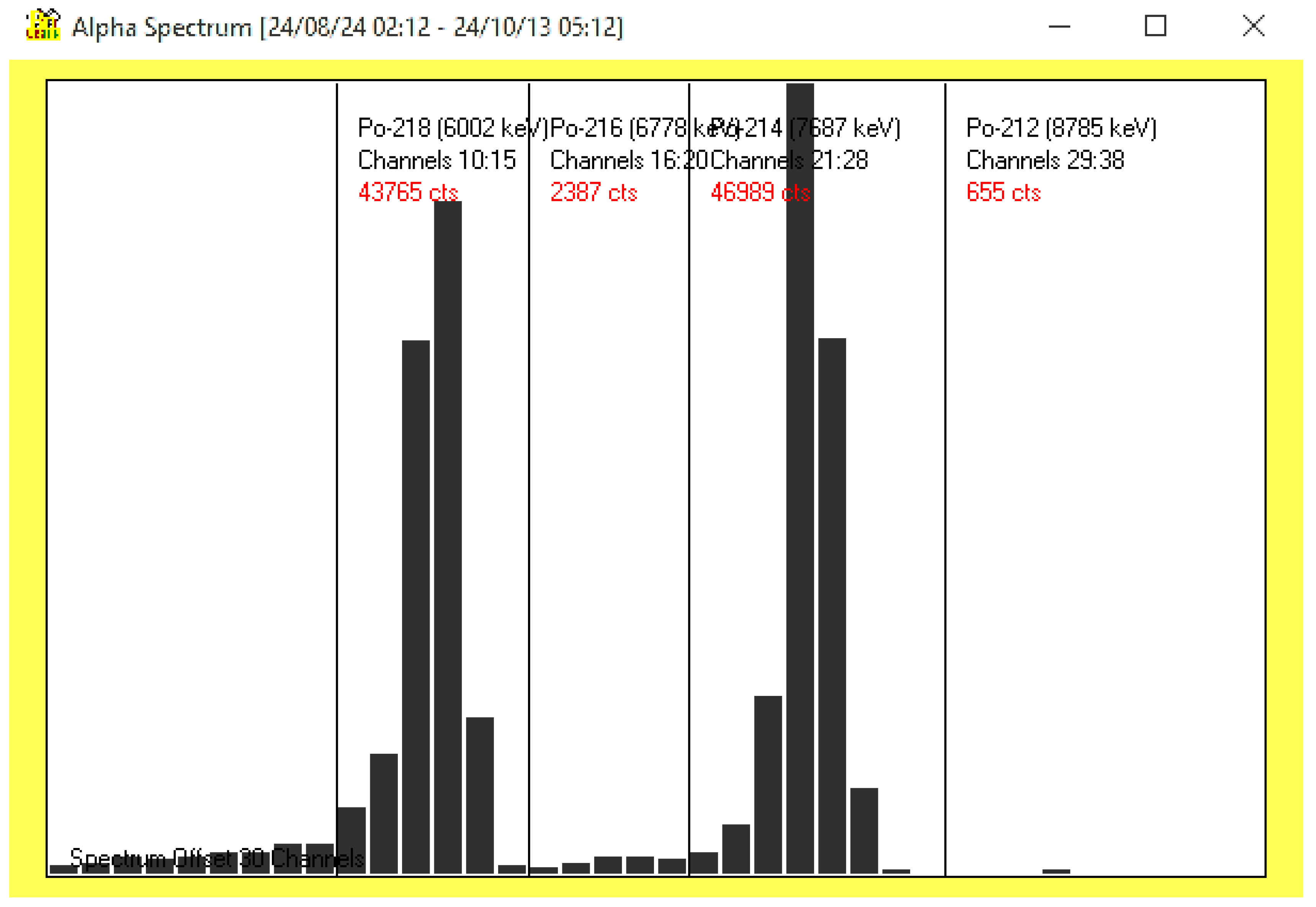
Figure 10.
Thoron in Plostina monitoring station (Radon Vision software).
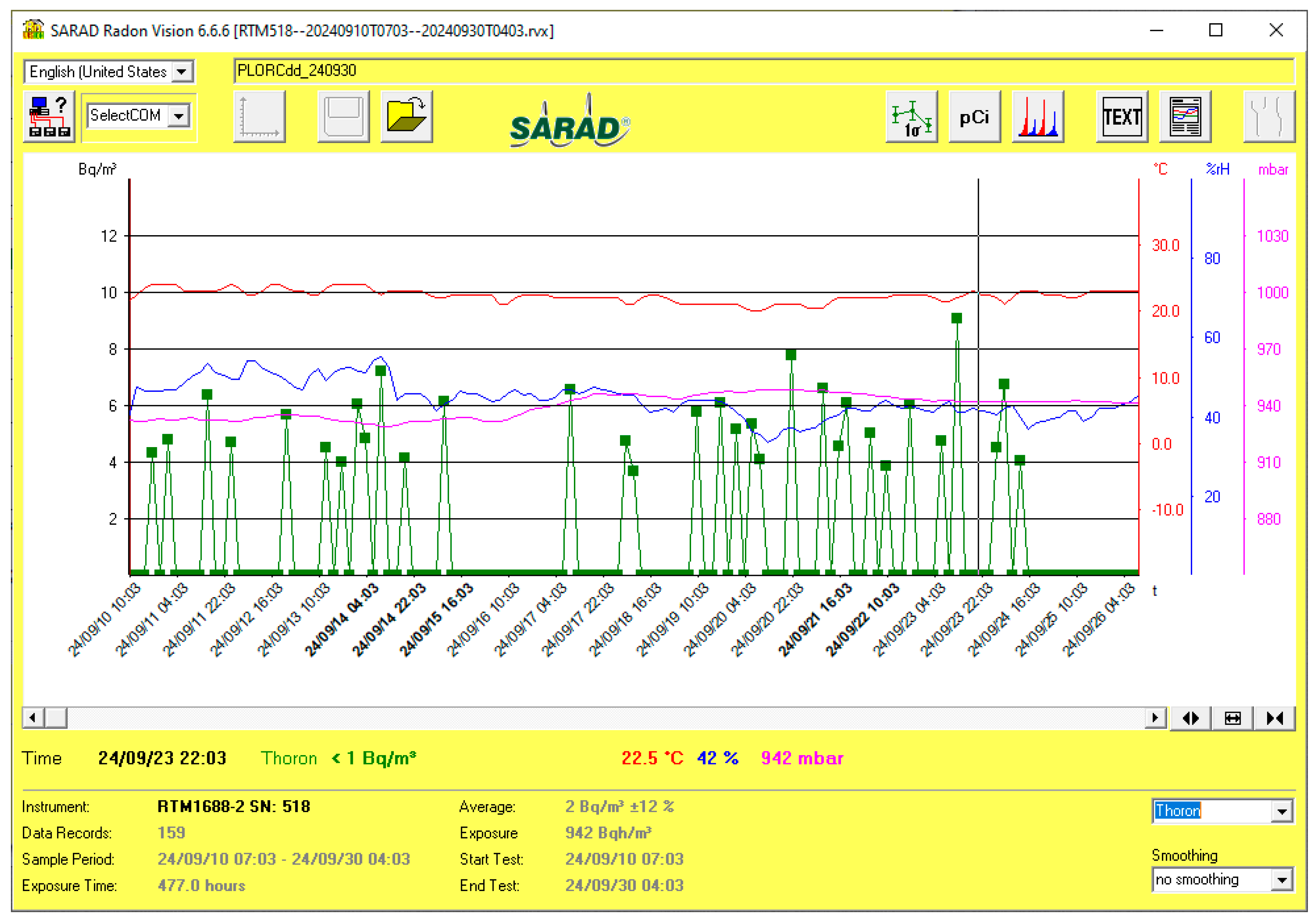
Figure 11.
Thoron in Vrancioaia station (Radon Vision software).
In conformity with SARAD’s User Manual Analogous Radon Sensor (Indoor Air Sensor / Soil Gas Sensor) Version 12/2007, the Radon concentration is linearly proportional to the number of detected decay events of the Po-218 (ROI2) and the Po-214 (ROI4). The Thoron concentration is linearly proportional to the number of detected Po-216 decays (ROI3). The calculation procedures are shown in the table below (User Manual Analogous Radon Sensor (Indoor Air Sensor / Soil Gas Sensor) Version 12/2007):

Table 5.
Calculation procedures for Radon and Thoron.
| ROI1 | ROI2 | ROI3 | ROI4 | ROI5 | Value | Calculation |
|---|---|---|---|---|---|---|
| - | X | - | - | - | Radon (fast) | CRn (fast) = N / (T * Sfast) |
| - | X | - | X | - | Radon (slow) | CRn (slow) = N / (T * Sslow) |
| - | - | - | X | - | Radon (Po-214 only) | CRn (Po-214) = N / (T *(Sslow – Sfast)) |
| - | - | X | - | - | Thoron | CTn = N / (T * SThoron) |
Where:
CRn—Radon concentration;
CTn—Thoron concentration;
-—ROI disabled;
X—ROI enabled;
N—Number of counts detected within all enabled ROI;
T—Time period used for counting;
S—Sensitivity (calibration constant stated within the calibration certificate).
So, radon is calculated from ROI2 (Po-218) and ROI4 (Po-214), Radon* fast from ROI2 (Po-218), Thoron from ROI3 (Po-216). The RTM1688-2 is more efficient than the Radon Scout Plus used until now, but more expensive and more difficult to maintain. In conformity with Radon Vision 7 User Guide, SARAD GmbH∗, December 9, 2020 ‘The energy ranges defined for calculating the radon measurement variables - also called regions of interest or ROI - are represented by vertical lines with the respective nuclide, the range limits and the counting pulses contained therein’, Figure 5 and Figure 6.
Methane is considered a seismic precursor in the Black Sea due to its peculiarities [18], also in the water in Costa Rica [19], or reflects the intensity status of tectonic activities [20,21].
Table 6 shows the CH4 equipment used in Vrancioaia and Plostina and Figure 12 a test with this equipment.
The tests will be done in Plostina, Vrancioaia, and Lopatari where there are live fires accompanied by the smell of gas and traces of oil on the ground. An air pump is required, which reduces system reliability and produces noise like the RTM1688-2. For this reason, the CH4 detector cannot be installed together with seismic sensors.
3. Analysis Methods and Results
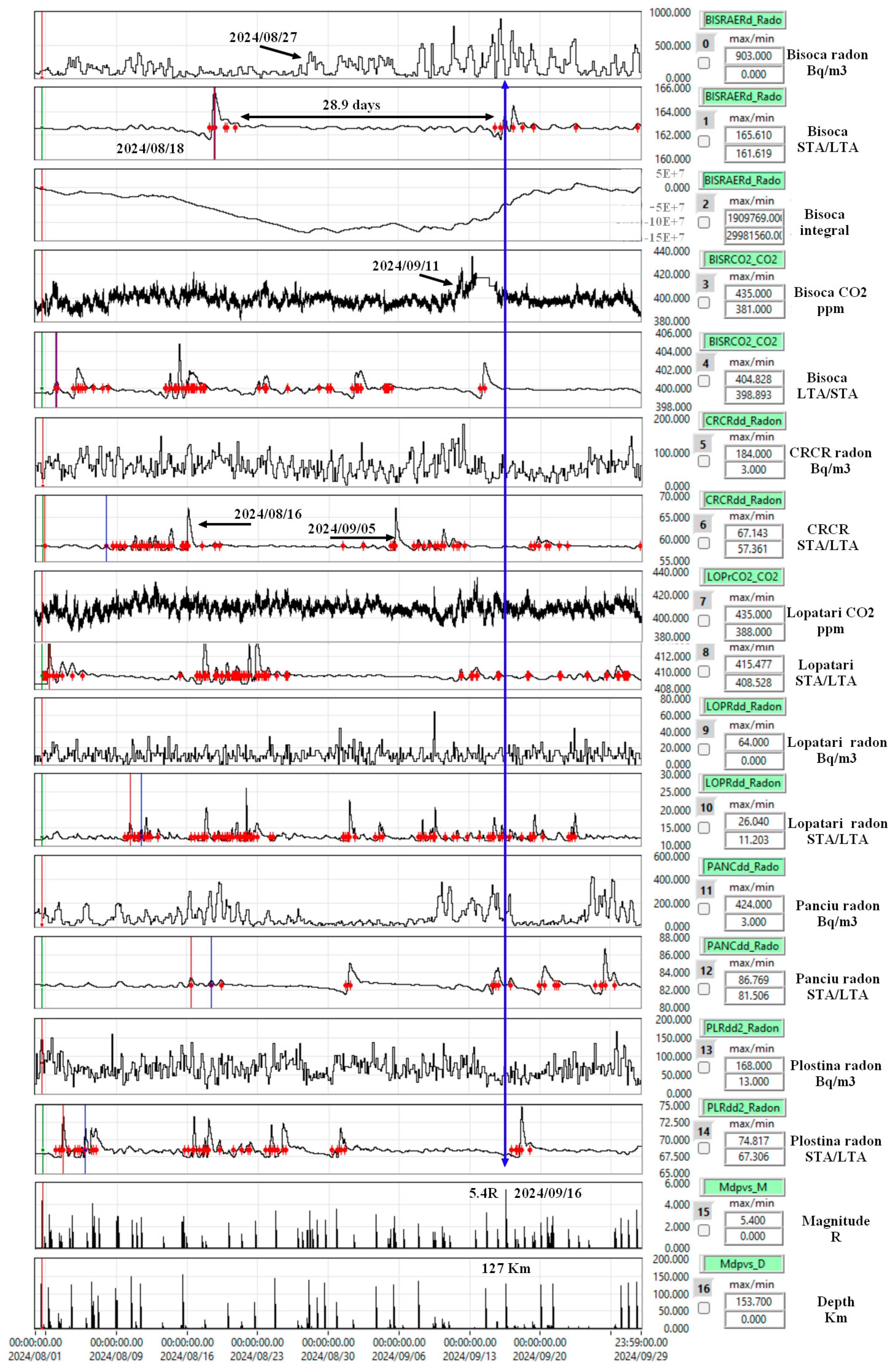
In this article, we check the analysis methods described in [2,3,4] after one year of monitoring. It is described in [2] "The logical tree of the forecast parameters of the Vrancea area" (Figure 16). The decision matrix and the comparative results of the detection methods used in this paragraph will be presented. The case study refers to the earthquake of 16.09.2024 with a magnitude of 5.4R (Figure 13). In Figure 13, the faults, the position of the epicenter, and distances to PLOR, PANC, BISRR, LOPR, and NEHR monitoring stations used in the Table 7 are marked.
The decision matrix is based on the number of detected events. In this example, the detection is based on exceeding some predefined thresholds, and the method is analyzed compared to the Allen-type STA/ LTA (Short-Term Averages/ Long-Term Averages) detection algorithm ([12,13,14]) applied to integrated signals after the average value has been extracted. Figure 14 refers to the level-based detection that is decentralized in the monitoring stations compared to the STA/LTA method in Figure 15 which uses large time series processed in the NIEP servers.
Figure 13.
Case study, the earthquake of 16.09.2024 with a magnitude of 5.4R.
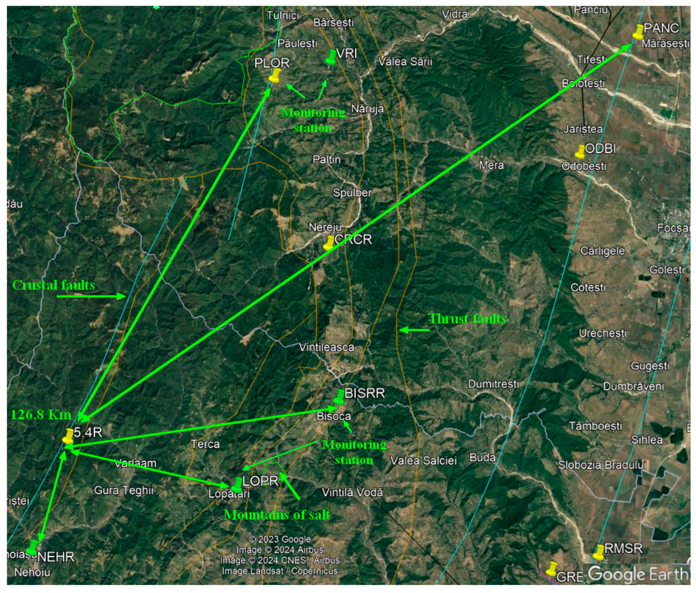
Figure 14.
The evolution of radon and CO2 before the 5.4R earthquakeand compared with the OEF AFROS decision matrix.
Figure 14.
The evolution of radon and CO2 before the 5.4R earthquakeand compared with the OEF AFROS decision matrix.
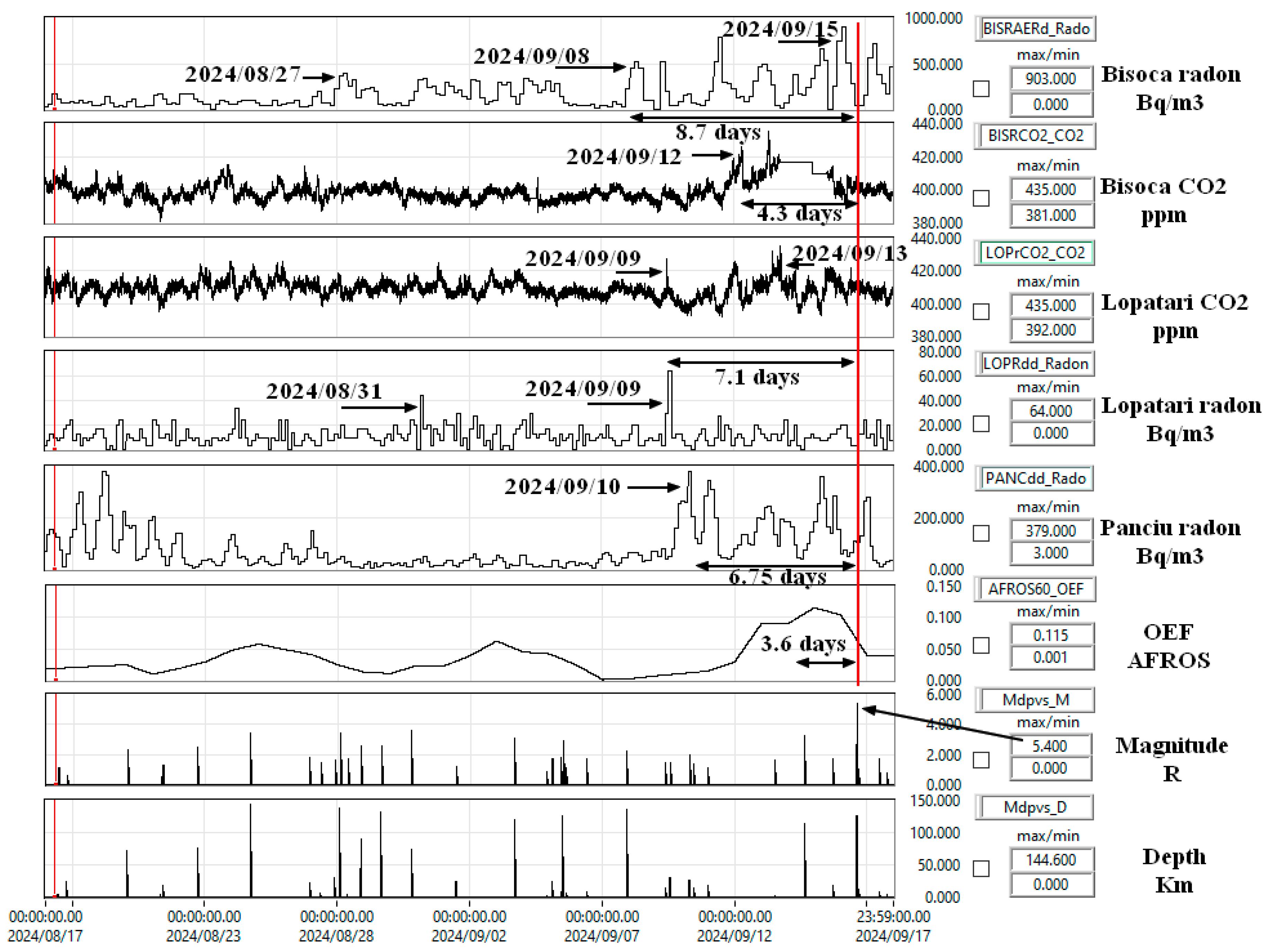
Figure 15.
The STA/LTA method was applied to the integrated radon and CO2 signals before the 5.4R earthquake and compared with the OEF AFROS decision matrix.
Figure 15.
The STA/LTA method was applied to the integrated radon and CO2 signals before the 5.4R earthquake and compared with the OEF AFROS decision matrix.
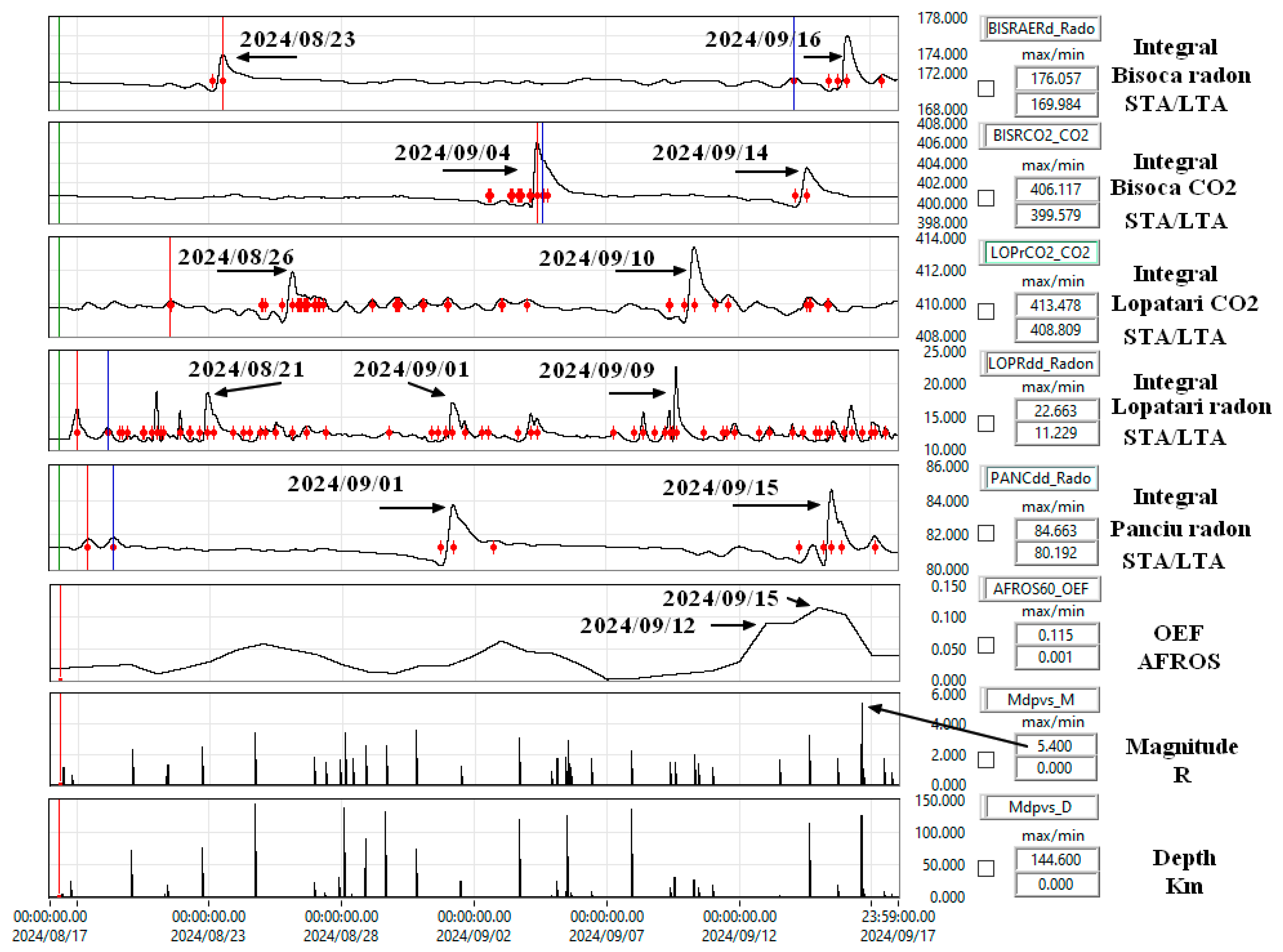
The result of the decision matrix (Table 7), referred to as OEF AFROS, shows an increase of 3.6 days before the earthquake according to Figure 14 and Figure 15. Figure 16 is a combination of these two figures but on a double time interval (2 months) before the 5.4R earthquake. The red points represent the detections by the STA/LTA method. Comparing these figures we can say that the time window of one month is sufficient for the decision matrix and that the method based on exceeding some thresholds works.
In the case of gas emissions (radon and CO2), we used the method of exceeding a level and returning below 99.96% on the first implementation. The result is a series of detections transmitted in real-time as Event files to the analysis server. Each station has a logical tree weighting, which was determined experimentally based on offline analyses. The maximum number of exceedances is 4 and was determined experimentally for Vrancea. It was also determined experimentally that for an earthquake of magnitude > 4R with the epicenter in Vrancea, an interval of 4 days corresponds to the detection groups for all stations. The result is shown in Table 7 and Figure 17, Figure 18 and refers to the earthquake of magnitude 5.4 R on 16.09.2024 based on monitoring station from Table 8.. In the example, the weights of the stations in the logical decision tree are equal and the number of stations is 8, the sum of the weights is 1. The algorithm allows their modification, the separation of radon and CO2 as weights, the modification of the weights according to the distance of the station from the hypocenter, the modification of the number of stations, the maximum number of detections per station in one day (4 in the example) and the 4-day drop-grouping period for all stations. Table 7 also includes seismicity in the Vrancea area. It is represented on the http://afros.infp.ro/AFROS.php?link=dategeofizice page as magnitude. We chose the cumulative energy/day , EnergyE, and mean Energy/4days in Figure 18 to include all the earthquakes of that day.
Figure 16.
Representation of two radon and CO2 months, time series, and integrated, STA/LTA detection marked with red dots.
Figure 16.
Representation of two radon and CO2 months, time series, and integrated, STA/LTA detection marked with red dots.
The decision matrix is based on relations (1 - 4).
Mean Day =SUM (Channel Weight0*exceedances0/maxim exceedances,
Channel Weightn-1*exceedancesn-1/maxim exceedances)/N stations
Channel Weightn-1*exceedancesn-1/maxim exceedances)/N stations
Mean m Daysn = SUM (Mean Dayn-3: Mean Dayn)/ m
The coefficients 11.4 and 1.5 are empirical and depend on the type of magnitude and location. Their values do not affect the method used. The measurement unit of seismic energy is Erg (ergi), 1 Erg = 10^–7 Joule.
1 = SUM (Channel Weights)
Table 7.
Decision matrix.
| Channel Weights | 0.125 | 0.125 | 0.125 | 0.125 | 0.125 | 0.125 | 0.125 | 0.125 | 1 | ||||
| Station | BISRAERd | BISRCO2 | DLMCO2 | DLMdd | LOPrCO2 | LOPRdd | NEHRdd | PANCdd |
Mean Day |
Mean 4 Days |
Mag R |
EnergyE *1E18 Erg |
EnergyE 4 Days *1E18 Erg |
| 2024/08/17 | 2 | 0 | 0 | 0 | 14 | 0 | 0 | 2 | 0.070312 | 0.0175781 | 1.2; 0.6 | 3.2562E-07 | 8.14048E-08 |
| 2024/08/18 | 0 | 0 | 0 | 0 | 0 | 0 | 0 | 3 | 0.011718 | 0.0205078 | 0 | 8.14048E-08 | |
| 2024/08/19 | 0 | 0 | 0 | 0 | 0 | 0 | 0 | 2 | 0.007812 | 0.0224609 | 0 | 8.14048E-08 | |
| 2024/08/20 | 0 | 0 | 0 | 0 | 0 | 0 | 0 | 2 | 0.007812 | 0.0244140 | 2.3 | 6.803E-07 | 2.51479E-07 |
| 2024/08/21 | 2 | 0 | 0 | 0 | 0 | 0 | 0 | 1 | 0.011718 | 0.0097656 | 0.5; 1.3 | 3.3849E-07 | 2.54696E-07 |
| 2024/08/22 | 2 | 0 | 0 | 0 | 10 | 0 | 0 | 0 | 0.046875 | 0.0185546 | 2.5 | 8.2662E-07 | 4.6135E-07 |
| 2024/08/23 | 0 | 0 | 0 | 0 | 13 | 0 | 0 | 0 | 0.050781 | 0.0292968 | 0 | 4.6135E-07 | |
| 2024/08/24 | 0 | 0 | 0 | 0 | 21 | 0 | 0 | 0 | 0.082031 | 0.0478515 | 3.4 | 1.9005E-06 | 7.664E-07 |
| 2024/08/25 | 0 | 0 | 0 | 0 | 13 | 0 | 0 | 0 | 0.050781 | 0.0576171 | 0 | 6.81778E-07 | |
| 2024/08/26 | 0 | 0 | 0 | 0 | 3 | 0 | 0 | 0 | 0.011718 | 0.0488281 | 1.8 | 4.1085E-07 | 5.77836E-07 |
| 2024/08/27 | 3 | 0 | 0 | 0 | 0 | 0 | 0 | 2 | 0.019531 | 0.0410156 | 1.5; 1.6 | 6.3309E-07 | 7.36108E-07 |
| 2024/08/28 | 2 | 0 | 0 | 0 | 2 | 0 | 0 | 0 | 0.015625 | 0.0244140 | 3.4; 1.7; 2.6 | 3.1807E-06 | 1.05615E-06 |
| 2024/08/29 | 1 | 0 | 0 | 0 | 0 | 0 | 0 | 0 | 0.003906 | 0.0126953 | 2.6 | 9.0991E-07 | 1.28363E-06 |
| 2024/08/30 | 1 | 0 | 0 | 0 | 0 | 0 | 0 | 0 | 0.003906 | 0.0107421 | 3.6 | 2.2661E-06 | 1.74745E-06 |
| 2024/08/31 | 0 | 0 | 0 | 0 | 18 | 0 | 0 | 0 | 0.070312 | 0.0234375 | 0 | 1.58918E-06 | |
| 2024/09/01 | 1 | 2 | 0 | 0 | 0 | 0 | 0 | 0 | 0.011718 | 0.0224609 | 1.2 | 2.1647E-07 | 8.48125E-07 |
| 2024/09/02 | 2 | 0 | 0 | 0 | 16 | 0 | 0 | 0 | 0.070312 | 0.0390625 | 0 | 6.20648E-07 | |
| 2024/09/03 | 3 | 0 | 0 | 0 | 22 | 0 | 0 | 0 | 0.097656 | 0.0625 | 3.1 | 1.451E-06 | 4.16859E-07 |
| 2024/09/04 | 0 | 0 | 0 | 0 | 0 | 0 | 0 | 0 | 0 | 0.0449218 | 0.9 | 0 | 4.16859E-07 |
| 2024/09/05 | 0 | 0 | 0 | 0 | 0 | 0 | 0 | 0 | 0 | 0.0419921 | 1.6; 1.7; 1.8; 2.9; 1.1 | 2.5152E-06 | 9.91554E-07 |
| 2024/09/06 | 0 | 0 | 0 | 0 | 0 | 0 | 0 | 0 | 0 | 0.0244140 | 1.7 | 3.7027E-07 | 1.08412E-06 |
| 2024/09/07 | 1 | 0 | 0 | 0 | 0 | 0 | 0 | 0 | 0.003906 | 0.0009765 | 2.2 | 6.1627E-07 | 8.75446E-07 |
| 2024/09/08 | 1 | 0 | 0 | 0 | 0 | 0 | 0 | 0 | 0.0039062 | 0.0019531 | 0 | 8.75446E-07 | |
| 2024/09/09 | 2 | 0 | 0 | 0 | 2 | 0 | 0 | 1 | 0.019531 | 0.0068359 | 1.5; 1.5 | 5.9951E-07 | 3.96511E-07 |
| 2024/09/10 | 2 | 0 | 0 | 0 | 0 | 0 | 0 | 2 | 0.015625 | 0.0107421 | 2; 1.4; 1.1 | 9.672E-07 | 5.45744E-07 |
| 2024/09/11 | 1 | 0 | 0 | 0 | 3 | 0 | 0 | 1 | 0.019531 | 0.0146484 | 0 | 3.91677E-07 | |
| 2024/09/12 | 2 | 4 | 0 | 0 | 9 | 0 | 0 | 1 | 0.0625 | 0.0292968 | 0 | 3.91677E-07 | |
| 2024/09/13 | 1 | 24 | 0 | 0 | 40 | 0 | 0 | 2 | 0.261718 | 0.0898437 | 0 | 2.41801E-07 | |
| 2024/09/14 | 0 | 0 | 0 | 0 | 2 | 0 | 0 | 2 | 0.015625 | 0.0898437 | 1.6 | 3.3334E-07 | 8.33342E-08 |
| 2024/09/15 | 1 | 0 | 0 | 0 | 28 | 0 | 0 | 2 | 0.121093 | 0.1152343 | 1.7 | 3.7027E-07 | 1.75902E-07 |
| 2024/09/16 | 2 | 0 | 0 | 0 | 2 | 0 | 0 | 1 | 0.019531 | 0.1044921 | 5.4; 1; | 9.9126E-06 | 2.65404E-06 |
| 2024/09/17 | 0 | 0 | 0 | 0 | 0 | 0 | 0 | 0 | 0 | 0.0390625 | 1.5; 0.8 | 4.3761E-07 | 2.76344E-06 |
| Total | 32 | 30 | 0 | 0 | 218 | 0 | 0 | 24 | |||||
Figure 17.
The result of the decision matrix based on level detections.
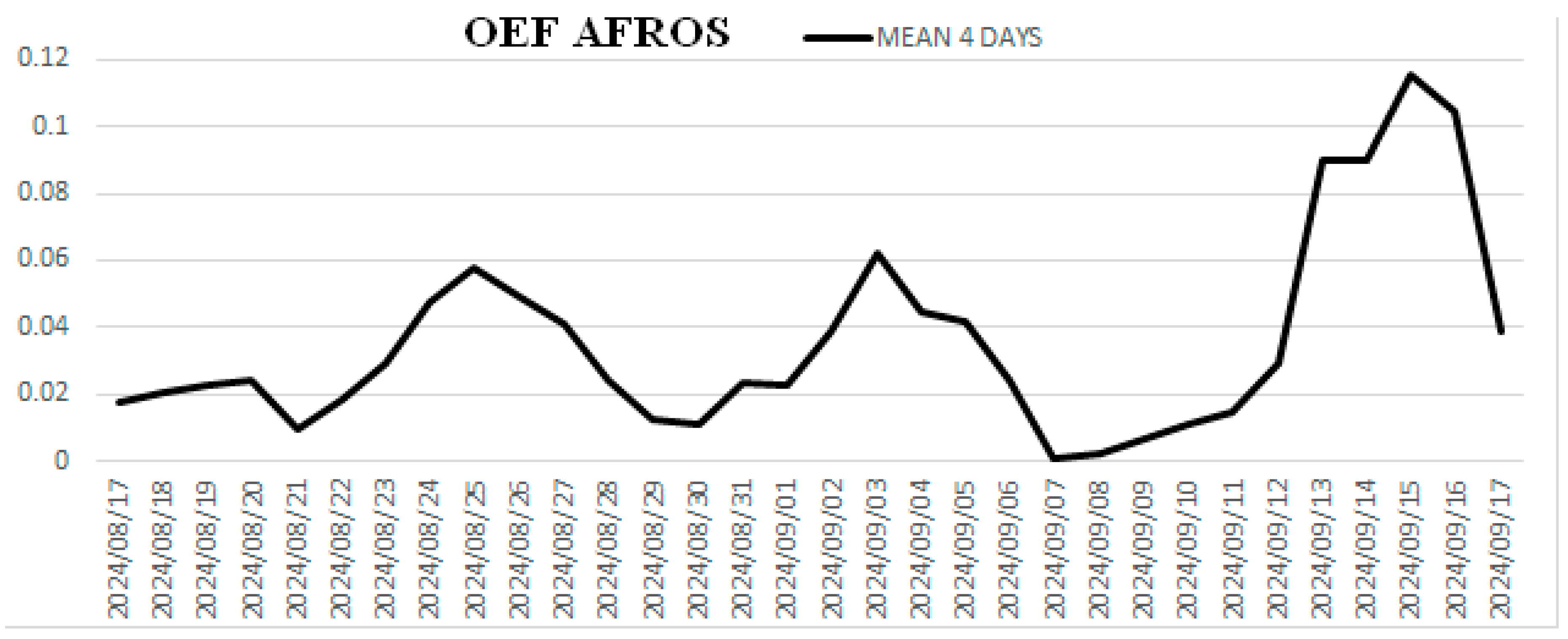
Figure 18 shows that 'EnergyE' is more intuitive than its mean on 4 days.
So, starting from the seismic Events file sent from monitoring stations we evaluate the possibility of having a seismic event. This is the simplest method to implement in our case because we made the data acquisition software and we can implement the detection algorithm.
An Events file example for radon in Bisoca station:
BISRAerd-Events_240911_091400.log -> 24/09/11 09:14:00 ROI1 5.920< 9.995
algorithm.
Figure 18.
Seismic energy cumulated/ day, EnergyE, and averaged over 4 days.
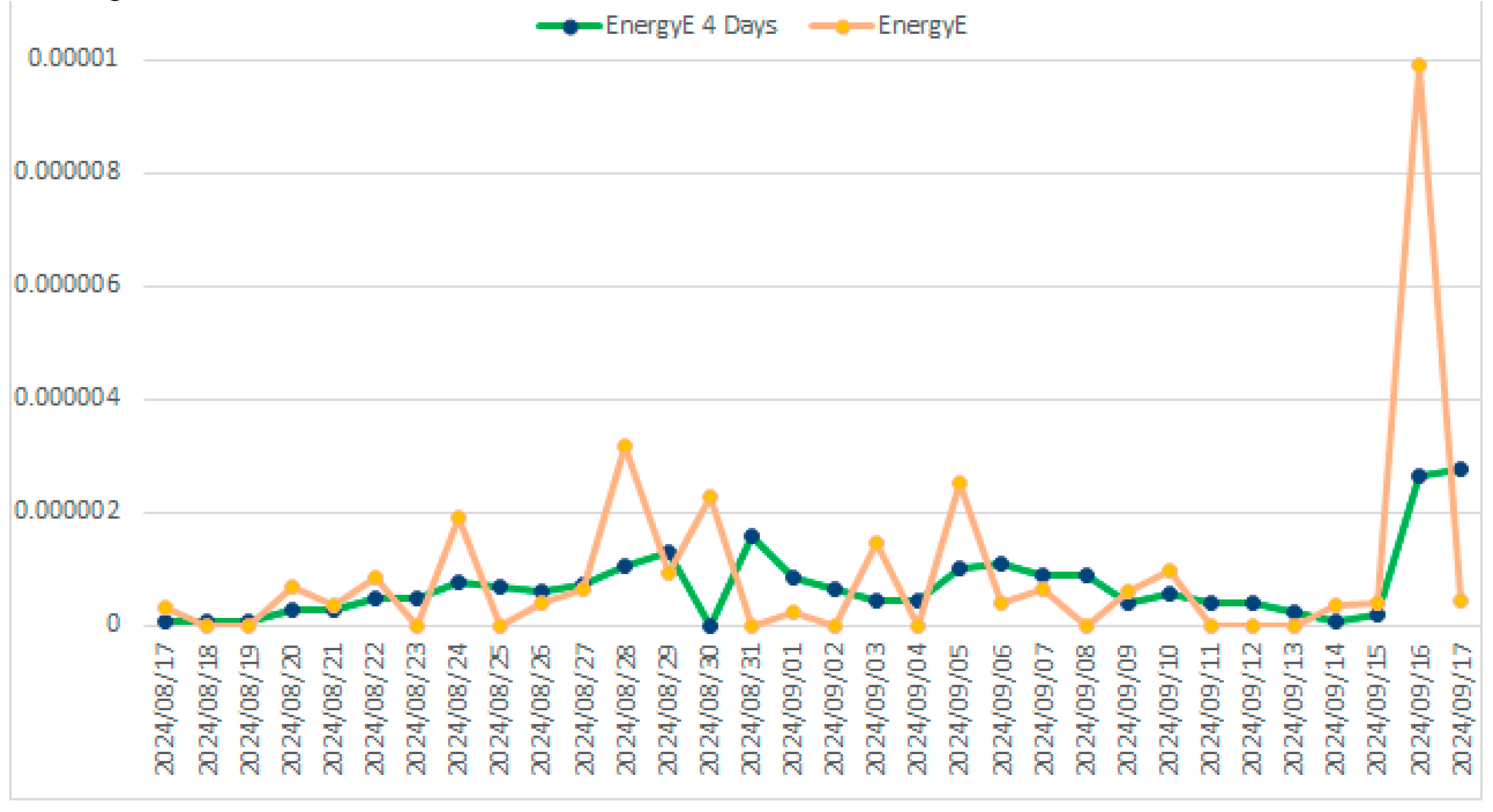
Table 8.
The monitoring stations used in the decision matrix.
| Station | Location | Equipment | North | East | Description | Start | End |
|---|---|---|---|---|---|---|---|
| BISRAERd | Bisoca | AERC | 45.5481 | 26.7099 | Biscoca, radon | 21/02/25 | - |
| BISRCO2 | Bisoca | DL303 | 45.5481 | 26.7099 | Bisoca CO2/CO | 19/07/09 | - |
| DLMCO2 | Dalma | DL303 | 45.3629 | 26.5965 | Dalma CO2/CO | 22/07/04 | _ |
| DLMdd | Dalma | RADONSCOUTp | 45.3629 | 26.5965 | Dalma, radon | 22/07/04 | _ |
| LOPrCO2 | Lopatari | DL303 | 45.4738 | 26.5680 | Mocearu, CO+CO2 | 19/06/26 | _ |
| LOPRdd | Lopatari | RADONSCOUTp | 45.4738 | 26.5680 | Mocearu, radon | 15/08/06 | _ |
| NEHRdd | Nehoiu | RADONSCOUTp | 45.4272 | 26.2952 | NEHR, radon | 15/08/06 | _ |
| PANCdd | Panciu | RADONSCOUTp | 45.8723 | 27.1477 | PANC, radon | 21/09/29 | _ |
4. Discussion
We will analyze the possibility of integration into the decision-making matrix of the monitoring stations in Plostina and Vrancioaia where new equipment has been installed. Software implemented at NIEP implements the data acquisition in real time only radon fast (Figure 19). This software allows the detection of exceeding thresholds and sends this information as an event. Figure 20 shows the contents of Figure 3 (Po-218) and Figure 4 (Po-214 + Po218) representing the radon in a room with the Radon Vision program (SARAD) in offline mode and the radon acquired with Radon Scout located in a pit. All figures refer to the same location, Plostina. It can be seen that there are no big differences between radon and radon fast (Figure 21), but its level in the pit (depth 50 cm) is significantly higher. Also, the evolution of radon in Plostina has no significant variations before the 5.4R earthquake of 16.09.2024, unlike the radon in Vrancioaia which indicates high values , especially after the earthquake (Figure 7 and Figure 8).
As in the case of radon, the Thoron from Plostina does not indicate a seismic event, but the one from Vrancioaia exceeds the trigger threshold and several red points appear in the STA/LTA graph (Figure 22).
The differences in the number of detections (Table 7, Figure 22) could be explained by the distance from the epicenter (Table 9). The epicentral area should not be regarded as a source of radon for the other monitoring stations, but the tectonic stress involves soil deformations that allow the gas emission to change. Table 7 shows that the most exceedances were for CO2 emissions from Lopatari, radon and CO2 from Bisoca, and radon from Panciu, following the epicentral distances. The stations used in Table 7 are the stations of the AFROS platform. The stations Dalma and Nehoiu did not function during that period, which would have required a change of the website by replacing them with other stations, which is not easy (the project is finished). Our ground deformation measurements used accelerometers used in seismic stations. They work as inclinometers at low frequencies. In areas where we have triaxial magnetometers, we use them because their offset depends on the position of the support to which they are attached. Regardless of which device is affected by the floor deformation, the dependence on temperature must be taken into account. Figure 23 shows the inclination of an Episensor accelerometer from Kinemetrics during the production of the 5.4R earthquake. Soil deformation, temperature, solar radiation, humidity and geological conditions determine the fluctuations in gas emissions ([30,31,32,33]). For this reason, a detector is installed in Vrancioaia to measure the air and ground temperature (Vaisala DST111) next to a pyranometer, and a net radiometer is installed in Plostina to determine the direct and reflected solar radiation and the ground temperature.
The OEF of NIEP also has a seismic component that was not included in the decision matrix in Table 7 but was mentioned in [2,4]. The seismicity from the period analyzed in Table 7 is presented in Table 10. We note that there are days when we have had several earthquakes (even 5 on 05.09.2024) that can be a seismic precursor, even if their magnitude is small. The Vrancea area is characterized by surface and deep earthquakes, which can also be seen in Table 10. The relationship between them is not yet defined, but the half-life of radon and thoron (Figure 1 and Figure 2) shows that the source of the gases must be on the surface. Figure 24 shows the decrease of the parameter "b" of the Gutenberg Richter law (GR_b) 29 days before the earthquake with a magnitude of 5.4R on 16.09.2024.
The decision matrix can also include other parameters such as ULF (Figure 23) or VLF (Figure 25) radio waves. Figure 25 also shows other factors related to local meteorological conditions (atmospheric pressure, temperature, wind, electrical discharges - EFM100C Boltek, magnetic storms - Kp). Table 11 shows the anomalies from Figure 25 of VLF waves.
A new receiver was instaled recenly in Plostina location.
Also, the electrical lighting could be a seismic precursor [27,29]. Figure 26 shows the storm on the earthquake day, but there is not a concentration over the epicenter area. This can be seen in Figure 25, the EFM 100C Boltek signal.
The decision matrix can be extended, but this requires an effort that must be seen through the prism of costs and benefits [11]. Only the parameters from the AFROS page http://afros.infp.ro/AFROS.php?link=dategeofizice are public in the OEF analysis, but the offline studies also involve other parameters and more stations.
4. Conclusions
OEF systems are complex because they sum up theories from many fields and implies a multidisciplinary approach. The main problem is the implementation of theoretical methods and data networks. Many methods depend on the specifics of the monitored area and must be adapted ([34,35,36,37]). An example is parameter b from the Gutenberg Richter law, which has a behavior specific to the Vrancea area, characterized by intermediate earthquakes. This fact is not found in Greece or Italy, with a high but crustal seismicity. The TURNkey project implemented an OEF, but the consortium that created it includes 21 partners from 10 European countries (funding from the European Union’s Horizon 2020 research and innovation program under grant agreement No 821046, https://cordis.europa.eu/project/id/821046). The AFROS project (PCE119/4.01.2021) also included fundamental research and the establishment of a seismic forecasting platform. The main problem is funding after completion of the projects for data support of the implemented platforms. In general, it is difficult to ensure the costs of maintaining the achievements of projects that do not have a beneficiary willing to continue financing. In this phase, the NIEP's OEF was limited to the public presentation of the use of gas emissions (radon and CO2) in a decision matrix related to seismicity in the Vrancea area. There are all the elements to expand the number and type of precursors. This can be achieved by extending the decision matrix or by creating further decision matrices depending on the grouping by data type. The data used must generate countable events that can be integrated in a platform. On the AFROS web page http://afros.infp.ro/AFROS.php?link=dategeofizice, seismic and magnetic data are also presented. Information about the water temperature in a borehole, radio waves in the ULF-VLF bands, etc. can also be added from NIEP’s data platform http://geobs.infp.ro. Another direction of development is the expansion of the area to be monitored and the type of progoza. Climatic changes are accompanied by large and rapid fluctuations in precipitation, temperatures, wind gusts, storms, etc.
From the experience of implementing an OEF, it can be concluded that its structure must be flexible to allow for its development. The more complex it is, the more difficult it will be to implement, maintain and finance. This is why the cost-benefit analysis is already important in the initial phase.
Author Contributions
Conceptualization, V.-E.T.; methodology, V.-E.T. and I.-A.M.; software, V.-E.T.; validation, A.M, and C.I.; formal analysis, I.-A.M. and M.A; investigation, V.-E.T. and I.-A.M.; writing—original draft preparation, V.-E.T.; correspondent, V.-E.T.; supervision, I.L. All authors have read and agreed to the published version of the manuscript.
Funding
This work was carried out within Nucleu Program project no PN23360101 and PN23360201.
Data Availability Statement
http://geobs.infp.ro, example of the data is archived at https://data.mendeley.com/datasets/28kv3gsgcz, Published: 27 September 2022|Version 2|DOI:10.17632/28kv3gsgcz.2.
Acknowledgments
This paper was carried out within Nucleu Program SOL4RISC, supported by MCI, projects no PN23360101 and PN23360201 and AFROS Project PN-III-P4-ID-PCE-2020-1361, supported by UEFISCDI.
Conflicts of Interest
The authors declare no conflict of interest.
References
- V.-E. V.-E. E. Toader, I.-A. I.-A. A. Moldovan, A. Marmureanu, P. K. R. R. P. K. R. Dutta, R. Partheniu, and E. Nastase, “Monitoring of radon and air ionization in a seismic area,” Rom. Reports Phys., vol. 69, no. 3, p. 842013, 2017.
- V.-E. Toader, V. Nicolae, I.-A. Moldovan, C. Ionescu, and A. Marmureanu, “Monitoring of Gas Emissions in Light of an OEF Application,” Atmosphere (Basel)., vol. 12, no. 1, p. 26, Dec. 2020. [CrossRef]
- V.-E. Toader, A. Mihai, I.-A. Moldovan, C. Ionescu, A. Marmureanu, and I. Lingvay, “Implementation of a Radon Monitoring Network in a Seismic Area,” Atmosphere (Basel)., vol. 12, no. 8, p. 1041, Aug. 2021. [CrossRef]
- V. E. Toader et al., “The Results and Developments of the Radon Monitoring Network in Seismic Areas,” Atmosphere (Basel)., vol. 14, no. 7, p. 1061, Jun. 2023. [CrossRef]
- T. Omi, Y. Ogata, K. Shiomi, B. Enescu, K. Sawazaki, and K. Aihara, “Implementation of a Real-Time System for Automatic Aftershock Forecasting in Japan,” Seismol. Res. Lett., vol. 90, no. 1, pp. 242–250, Jan. 2019. [CrossRef]
- A. Christophersen et al., “Progress and challenges in operational earthquake forecasting in New Zealand,” in 2017 NZSEE Conference, 2017, pp. 1–6, [Online]. Available: http://db.nzsee.org.nz/2017/O3C.4_Christophersen.pdf.
- L. Mizrahi et al., “Developing, Testing, and Communicating Earthquake Forecasts: Current Practices and Future Directions,” Rev. Geophys., vol. 62, no. 3, pp. 1–70, Sep. 2024. [CrossRef]
- Z. H. El-Isa and D. W. Eaton, “Spatiotemporal variations in the b-value of earthquake magnitude–frequency distributions: Classification and causes,” Tectonophysics, vol. 615–616, pp. 1–11, Mar. 2014. [CrossRef]
- W. D. Smith, “The b-value as an earthquake precursor,” Nature, vol. 289, no. 5794, pp. 136–139, Jan. 1981. [CrossRef]
- Thomas H. et al., “OPERATIONAL EARTHQUAKE FORECASTING. State of Knowledge and Guidelines for Utilization,” Ann. Geophys., vol. 54, no. 4, pp. 319–391, Aug. 2011. [CrossRef]
- J. Douglas and A. Azarbakht, “Cost–benefit analyses to assess the potential of Operational Earthquake Forecasting prior to a mainshock in Europe,” Nat. Hazards, vol. 105, no. 1, pp. 293–311, 2021. [CrossRef]
- V. R. E. X. Allen, “AUTOMATIC EARTHQUAKE RECOGNITION AND TIMING FROM Single Traces,” Bull. Seismol. Soc. Americ, vol. 68, no. 5, pp. 1521–1532, 1978.
- R. Allen, “Automatic phase pickers: Their present use and future prospects,” Bull. Seismol. Soc. Am. | Geosci., vol. 72, no. 6B, pp. 225–S242, 1982, Accessed: Apr. 28, 2020. [Online]. Available: https://pubs.geoscienceworld.org/ssa/bssa/article-abstract/72/6B/S225/102172/Automatic-phase-pickers-Their-present-use-and?redirectedFrom=fulltext.
- J. P. Jones and M. van der Baan, “Adaptive STA–LTA with Outlier Statistics,” Bull. Seismol. Soc. Am., vol. 105, no. 3, pp. 1606–1618, Jun. 2015. [CrossRef]
- Y. Hwa Oh and G. Kim, “A radon-thoron isotope pair as a reliable earthquake precursor,” Sci. Rep., vol. 5, no. 1, p. 13084, Aug. 2015. [CrossRef]
- H. P. Jaishi, S. Singh, R. P. Tiwari, and R. C. Tiwari, “Temporal variation of soil radon and thoron concentrations in Mizoram (India), associated with earthquakes,” Nat. Hazards, vol. 72, no. 2, pp. 443–454, 2014. [CrossRef]
- G. K. Gillmore, R. G. M. Crockett, and T. A. Przylibski, “IGCP Project 571: Radon, Health and Natural Hazards,” Nat. Hazards Earth Syst. Sci., vol. 10, no. 10, pp. 2051–2054, Oct. 2010. [CrossRef]
- A. Vasilev et al., “New Possible Earthquake Precursor and Initial Area for Satellite Monitoring,” Front. Earth Sci., vol. 8, no. February, pp. 1–9, 2021. [CrossRef]
- S. Mau, G. Rehder, I. G. Arroyo, J. Gossler, and E. Suess, “Indications of a link between seismotectonics and CH4 release from seeps off Costa Rica,” Geochemistry, Geophys. Geosystems, vol. 8, no. 4, 2007. [CrossRef]
- X. Wang et al., “Analysis of Seismic Methane Anomalies at the Multi-Spatial and Temporal Scales,” Remote Sens., vol. 16, no. 12, p. 2175, Jun. 2024. [CrossRef]
- Y. Huang, J. Cui, Z. Zhima, D. Jiang, X. Wang, and L. Wang, “Construction of a Fine Extraction Process for Seismic Methane Anomalies Based on Remote Sensing: The Case of the 6 February 2023, Türkiye–Syria Earthquake,” Remote Sens., vol. 16, no. 16, p. 2936, Aug. 2024. [CrossRef]
- C. F. Richter, “Elementary seismology,” Geol. J., vol. 2, no. 2, p. 768, Jan. 1958. [CrossRef]
- M. Båth, “Earthquake seismology,” Earth-Science Rev., vol. 1, no. 1, pp. 69–86, Jan. 1966. [CrossRef]
- M. Båth, “Seismic energy mapping applied to Turkey,” Tectonophysics, vol. 82, no. 1–2, pp. 69–87, Feb. 1982. [CrossRef]
- A. Nina, “VLF Signal Noise Reduction during Intense Seismic Activity: First Study of Wave Excitations and Attenuations in the VLF Signal Amplitude,” Remote Sens., vol. 16, no. 8, p. 1330, Apr. 2024. [CrossRef]
- A. Nina, “Analysis of VLF Signal Noise Changes in the Time Domain and Excitations/Attenuations of Short-Period Waves in the Frequency Domain as Potential Earthquake Precursors,” Remote Sens., vol. 16, no. 2, 2024. [CrossRef]
- M. Kachakhidze and N. Kachakhidze-Murphy, “VLF/LF Electromagnetic Emissions Predict an Earthquake,” Open J. Earthq. Res., vol. 11, no. 02, pp. 31–43, 2022. [CrossRef]
- H. Eichelberger et al., “INVESTIGATION OF VLF / LF ELECTRIC FIELD VARIATIONS RELATED TO MAGNITUDE MW ≥ 5. 5 EARTHQUAKES IN THE MEDITERRANEAN REGION FOR THE YEAR 2023,” no. April, pp. 1–9, 2024.
- L. V. Sorokin, “Lightning triggering related with seismic waves,” 7th Int. Symp. Electromagn. Compat. Electromagn. Ecol. Proceedings, EMCECO 2007, no. February, pp. 297–300, 2007. [CrossRef]
- P. Tuccimei, S. Mollo, M. Soligo, P. Scarlato, and M. Castelluccio, “Real-time setup to measure radon emission during rock deformation: implications for geochemical surveillance,” Geosci. Instrumentation, Methods Data Syst., vol. 4, no. 1, pp. 111–119, May 2015. [CrossRef]
- H. L. S.J. Bauer, W.P. Gardner, “Real Time Degassing of Rock during Deformation,” in 50th US Rock Mechanics / Geomechanics Symposium held in Houston, TX, USA, 2016, pp. 1–7, [Online]. Available: file:///C:/Users/C57.DESKTOP-ML0C8QK.000/Downloads/Bauer et al.%252c2016_ARMA.pdf.
- F. Ambrosino, L. Thinová, M. Briestenský, F. Giudicepietro, V. Roca, and C. Sabbarese, “Analysis of geophysical and meteorological parameters influencing 222Rn activity concentration in Mladeč caves (Czech Republic) and in soils of Phlegrean Fields caldera (Italy),” Appl. Radiat. Isot., vol. 160, p. 109140, Jun. 2020. [CrossRef]
- N. Morales-Simfors, R. A. Wyss, and J. Bundschuh, “Recent progress in radon-based monitoring as seismic and volcanic precursor: A critical review,” Crit. Rev. Environ. Sci. Technol., vol. 50, no. 10, pp. 979–1012, May 2020. [CrossRef]
- V. Emilian Toader, V. I.-A. M. I. C. A. M. A. M. Toader, A. Mihai, and A. Toader, V.E.; Moldovan, I.A; Mihai, “Forecast Earthquake Using Acoustic Emission,” in International Multidisciplinary Scientific GeoConference Surveying Geology and Mining Ecology Management, SGEM, Jun. 2019, vol. 19, no. 1.1, pp. 803–811. [CrossRef]
- N. Kachakhidze-Murphy, M. Kachakhidze, and P. F. Biagi, “Earthquake Forecasting Possible Methodology,” GESJ Phys., vol. 1, no. 15, pp. 102–111, 2016, [Online]. Available: http://gesj.internet-academy.org.ge/download.php?id=2790.pdf&t=1.
- J. D. Zechar, W. Marzocchi, and S. Wiemer, “Operational earthquake forecasting in Europe: progress, despite challenges,” Bull. Earthq. Eng., vol. 14, no. 9, pp. 2459–2469, Sep. 2016. [CrossRef]
- Thomas H. et al., “OPERATIONAL EARTHQUAKE FORECASTING. State of Knowledge and Guidelines for Utilization,” Ann. Geophys., vol. 54, no. 4, Aug. 2011. [CrossRef]
Figure 1.
‘The Basic Radon (222Rn) Decay Chain. The isotopes and their atomic masses are shown within the boxes; the main decay processes are indicated by arrows, with the type of decay and half-life indicated’ [17]
Figure 1.
‘The Basic Radon (222Rn) Decay Chain. The isotopes and their atomic masses are shown within the boxes; the main decay processes are indicated by arrows, with the type of decay and half-life indicated’ [17]
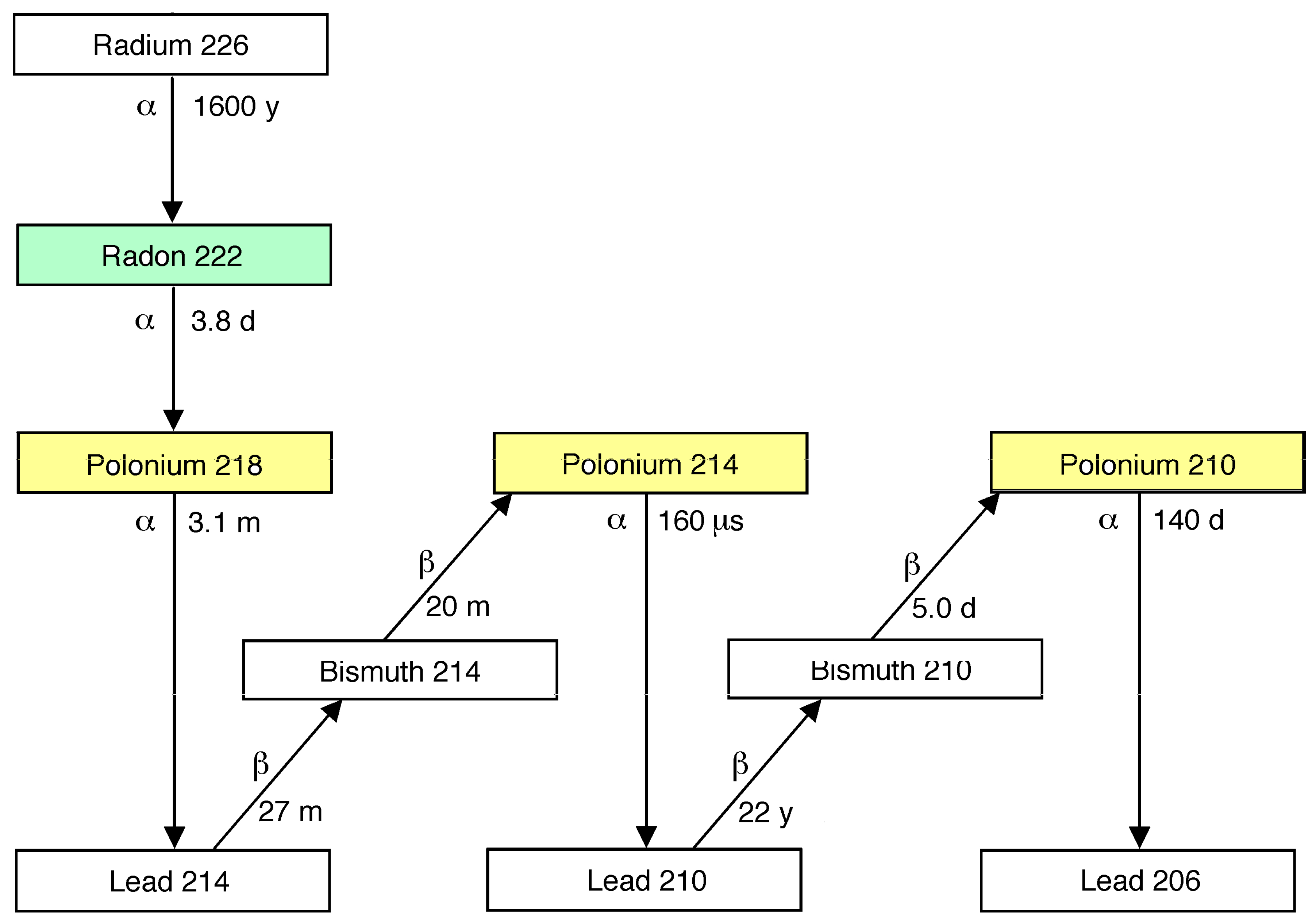
Figure 2.
Thorium (232Th) decay chain.
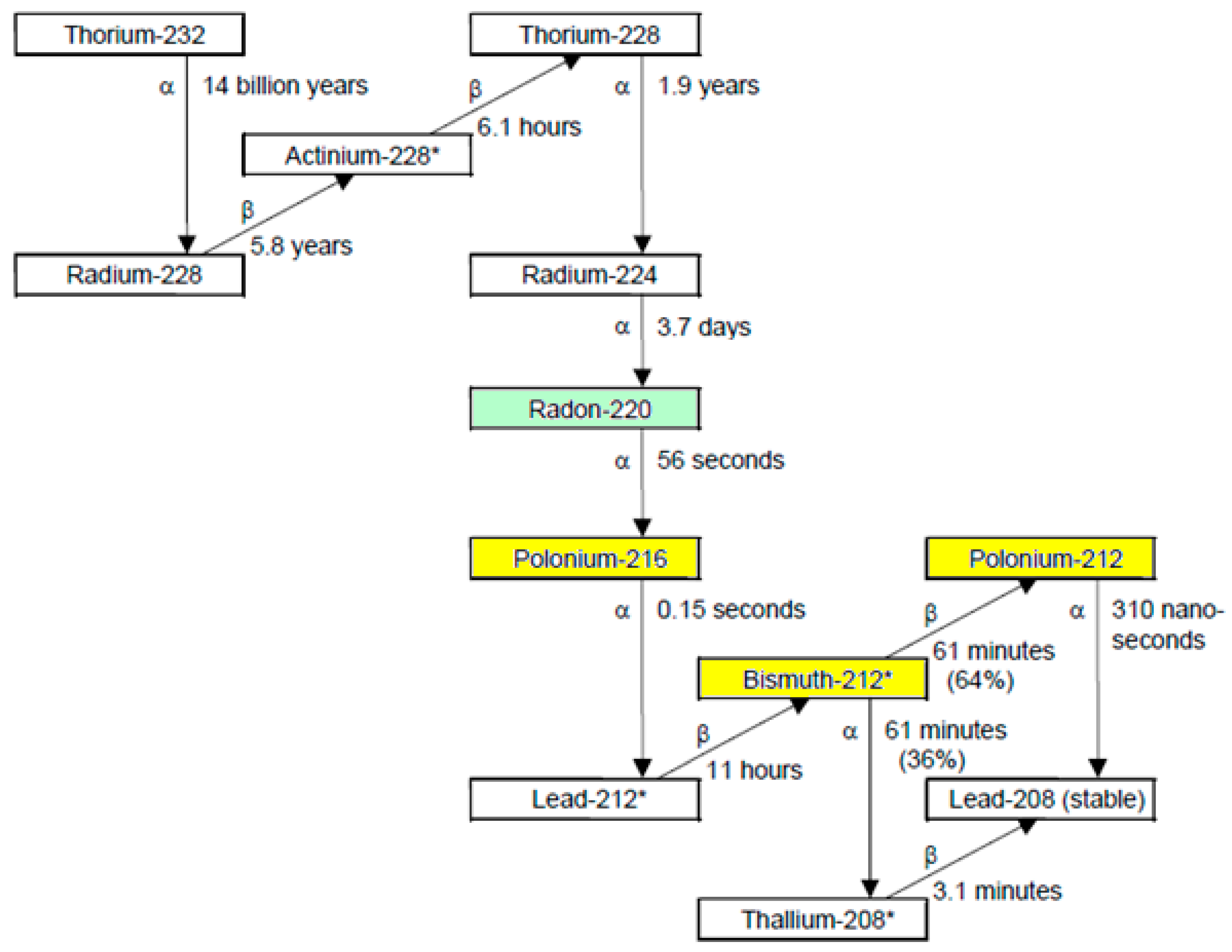
Figure 12.
Test with Chill Card NG Infrared Gas Sensor, Edinburgh Sensors UK.
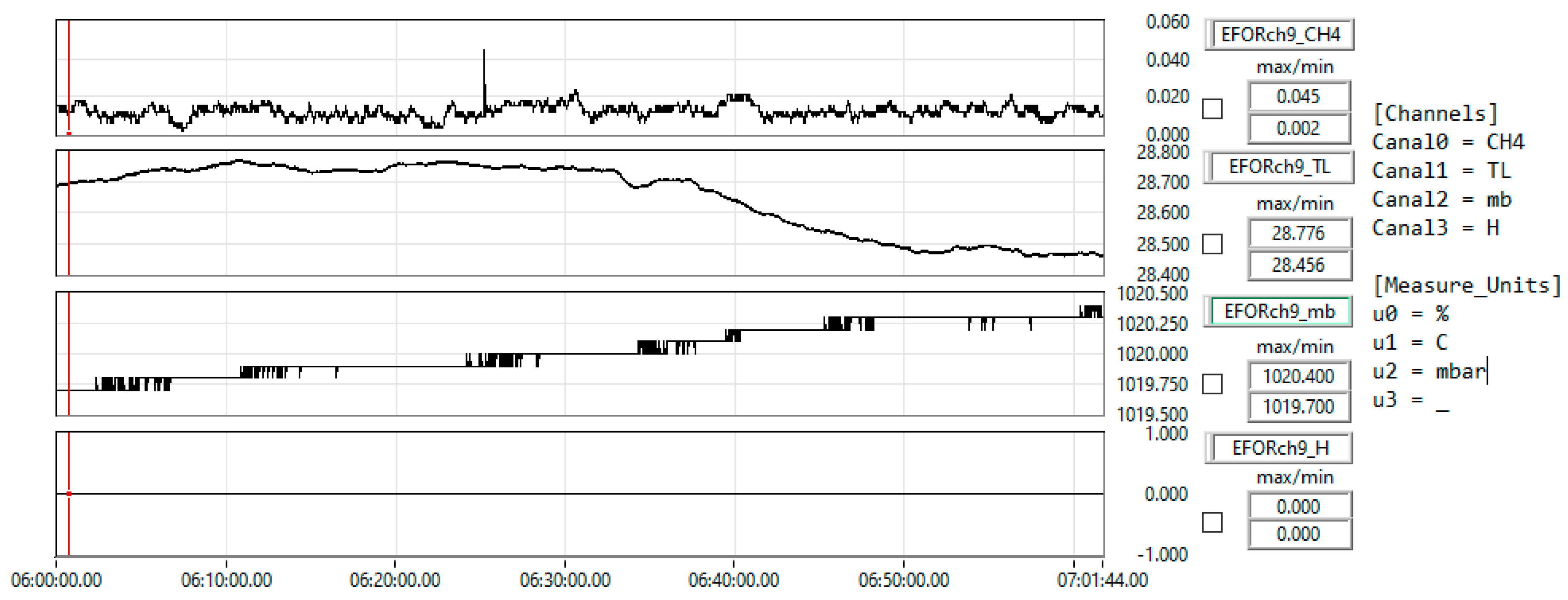
Figure 19.
Software for data acquistion RTM1688-2.
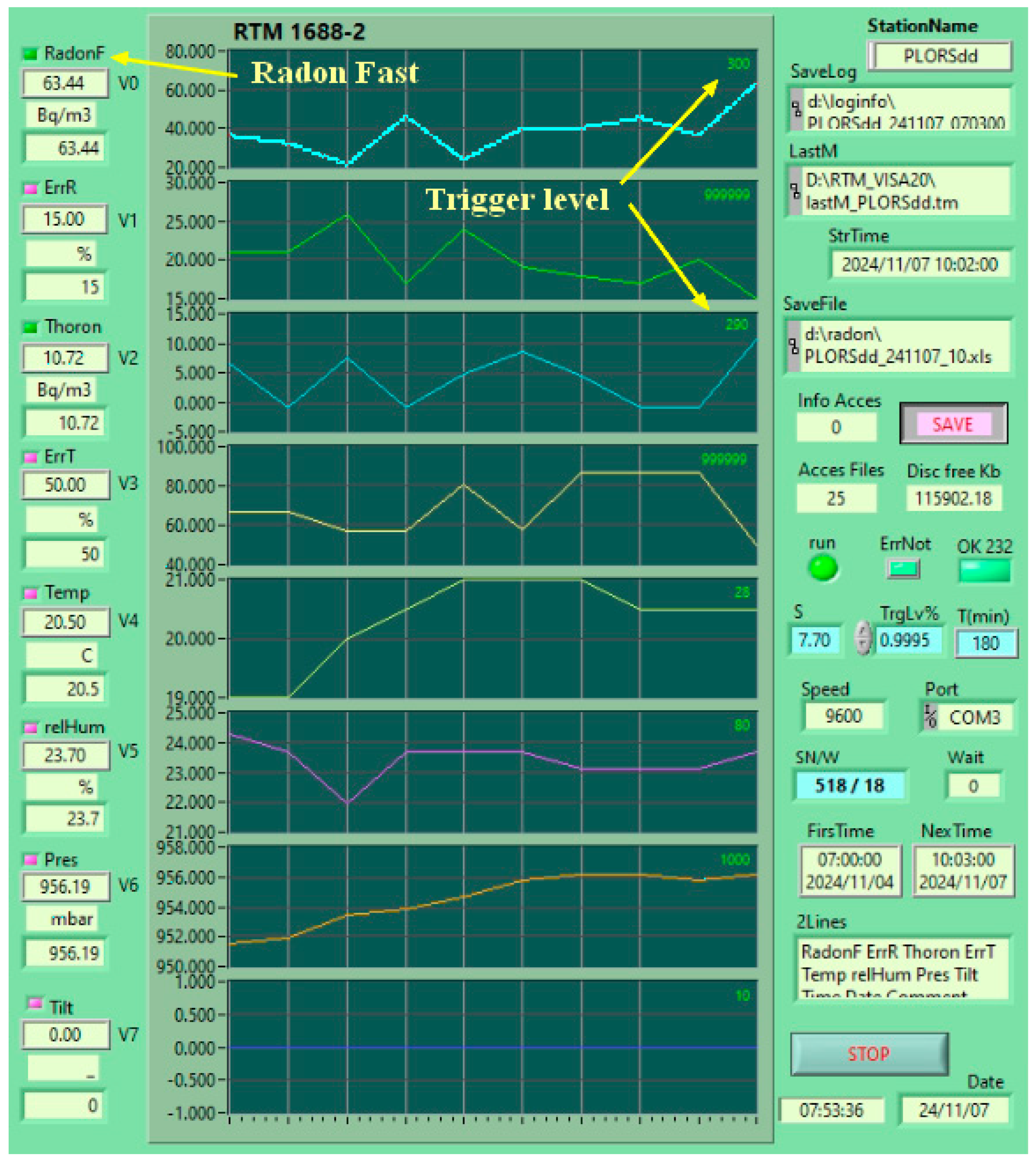
Figure 20.
Radon, Radon*(fast) RTM1688, Radon fast Radon Scout, Plostina.
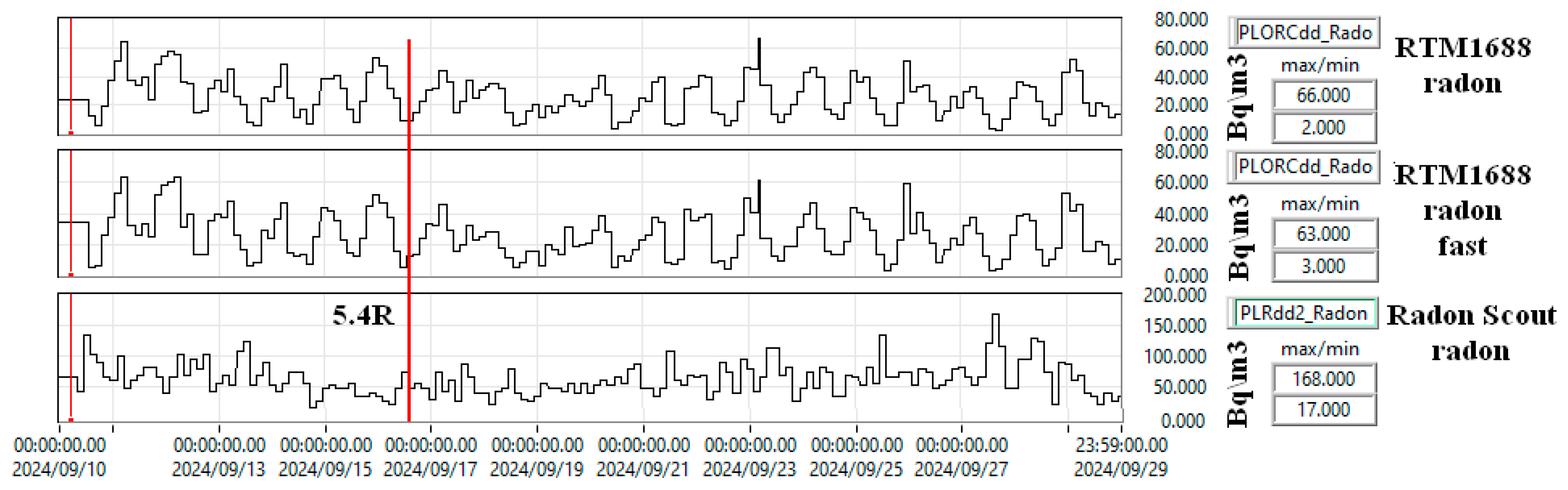
Figure 21.
Radon* (fast) evolution in Plostina site, RTM1688 data (Radon Vision software).
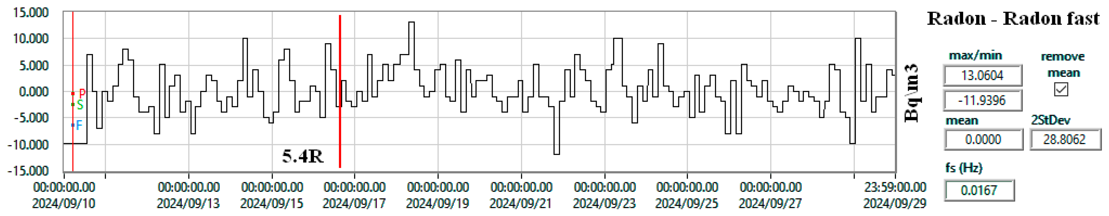
Figure 22.
Analysis of Thoron as a seismic precursor in Plostina and Vrancioaia.
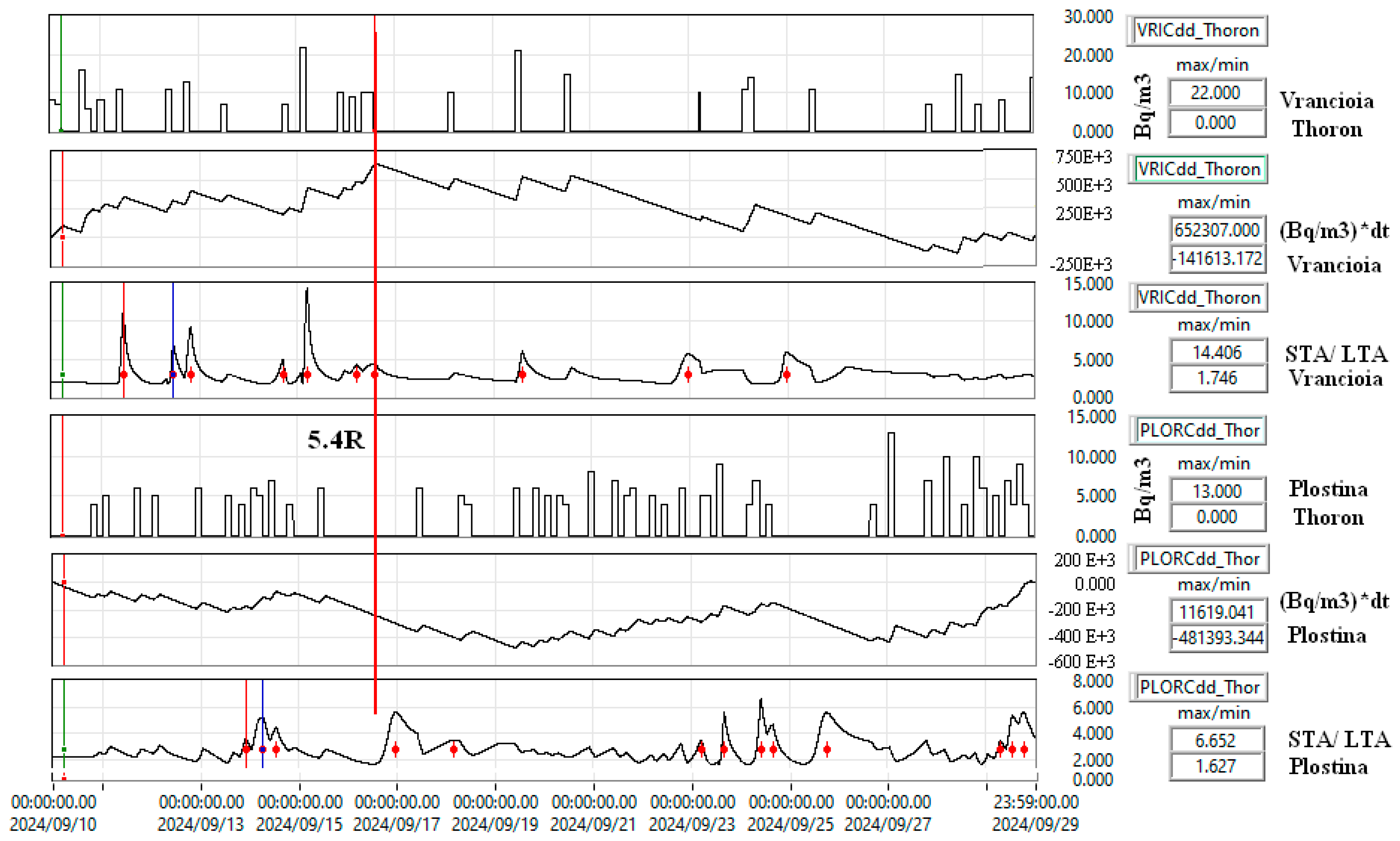
Figure 23.
Soil deformation was determined by an accelerometer before the 5.4R earthquake.
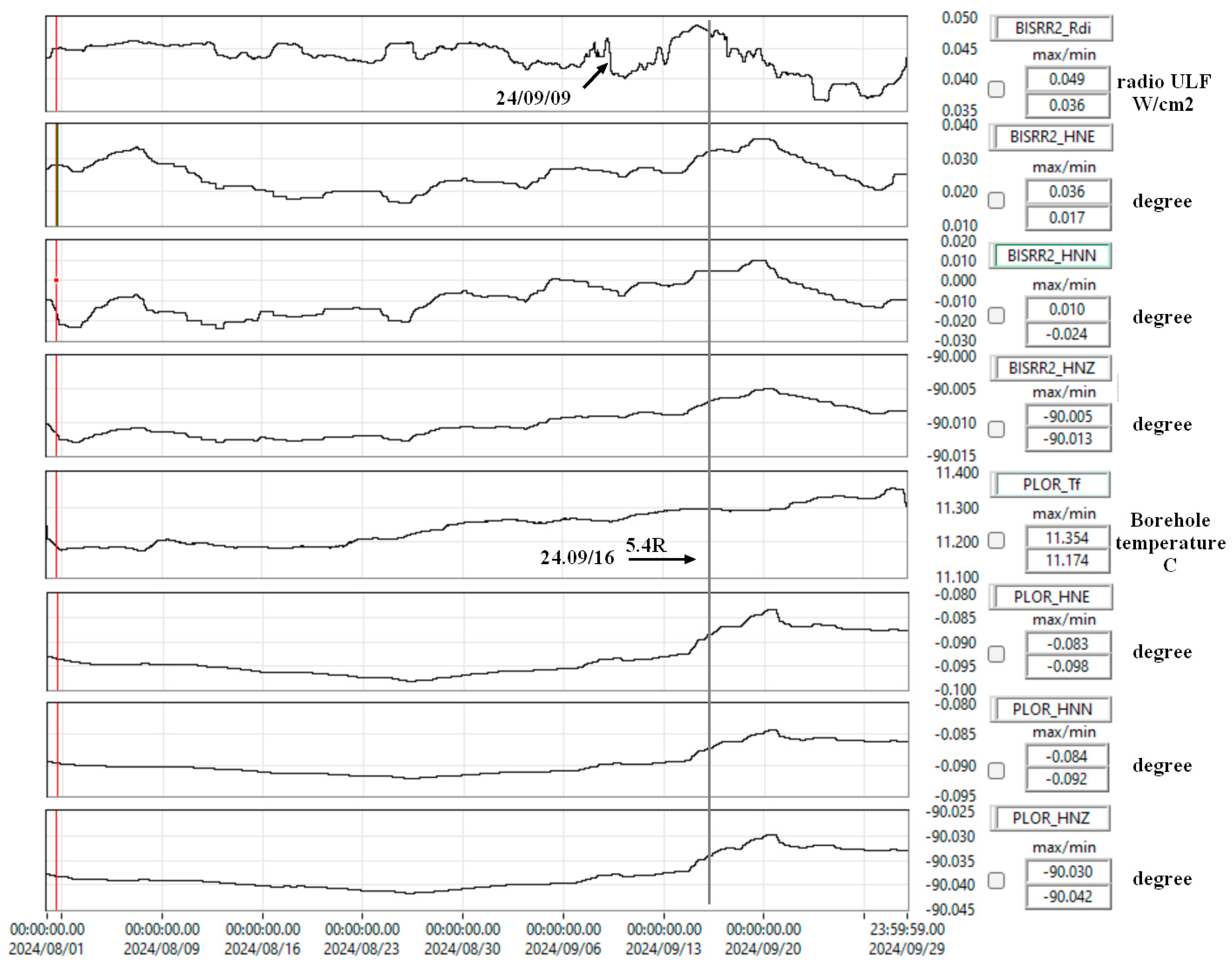
Figure 24.
The seismicity of the Vrancea area, the "b" parameter from the Gutenberg-Richter law (GR_b), seismic energy.
Figure 24.
The seismicity of the Vrancea area, the "b" parameter from the Gutenberg-Richter law (GR_b), seismic energy.
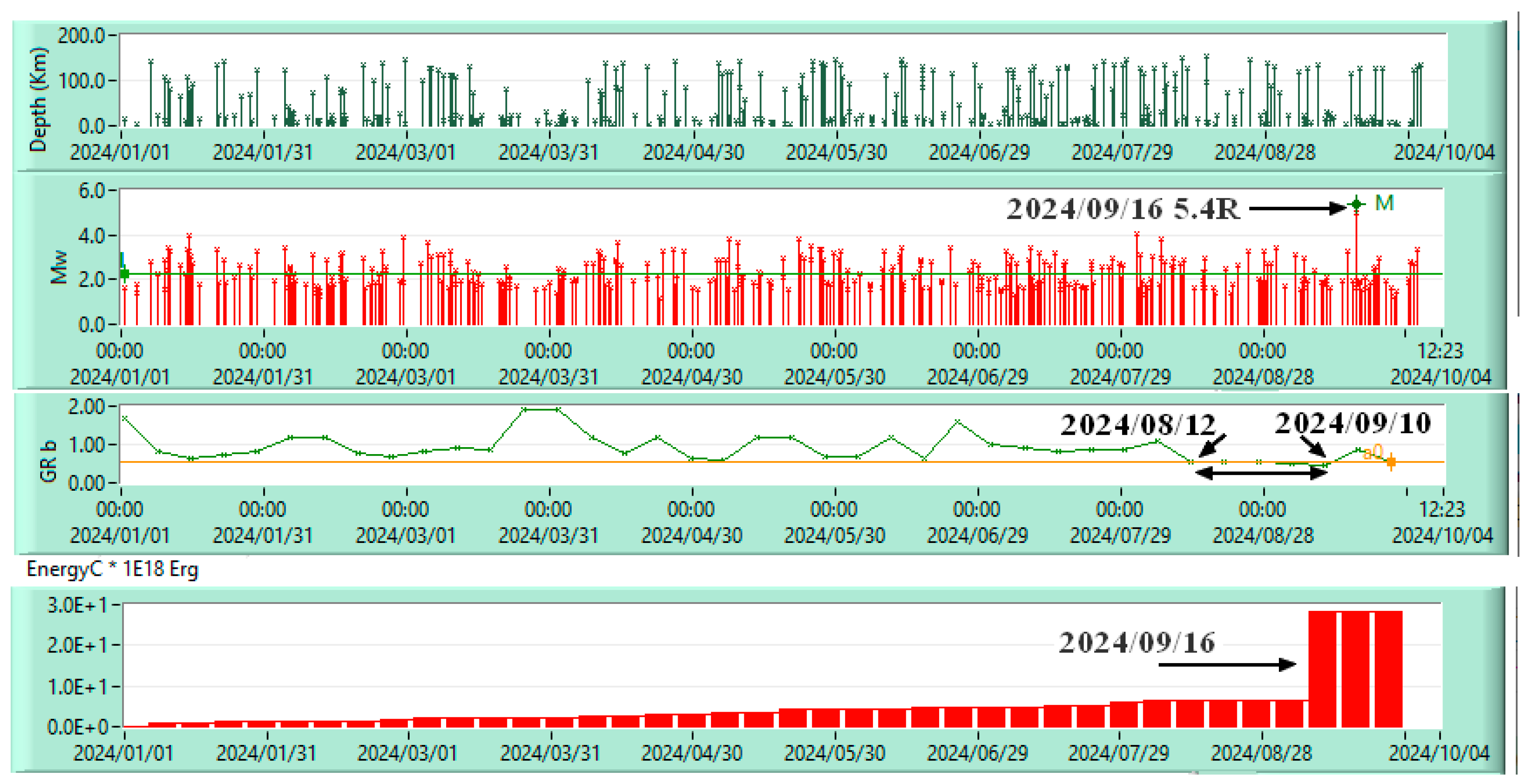
Figure 25.
Meteorological, VLF, and Kp data before the 5.4R earthquake.
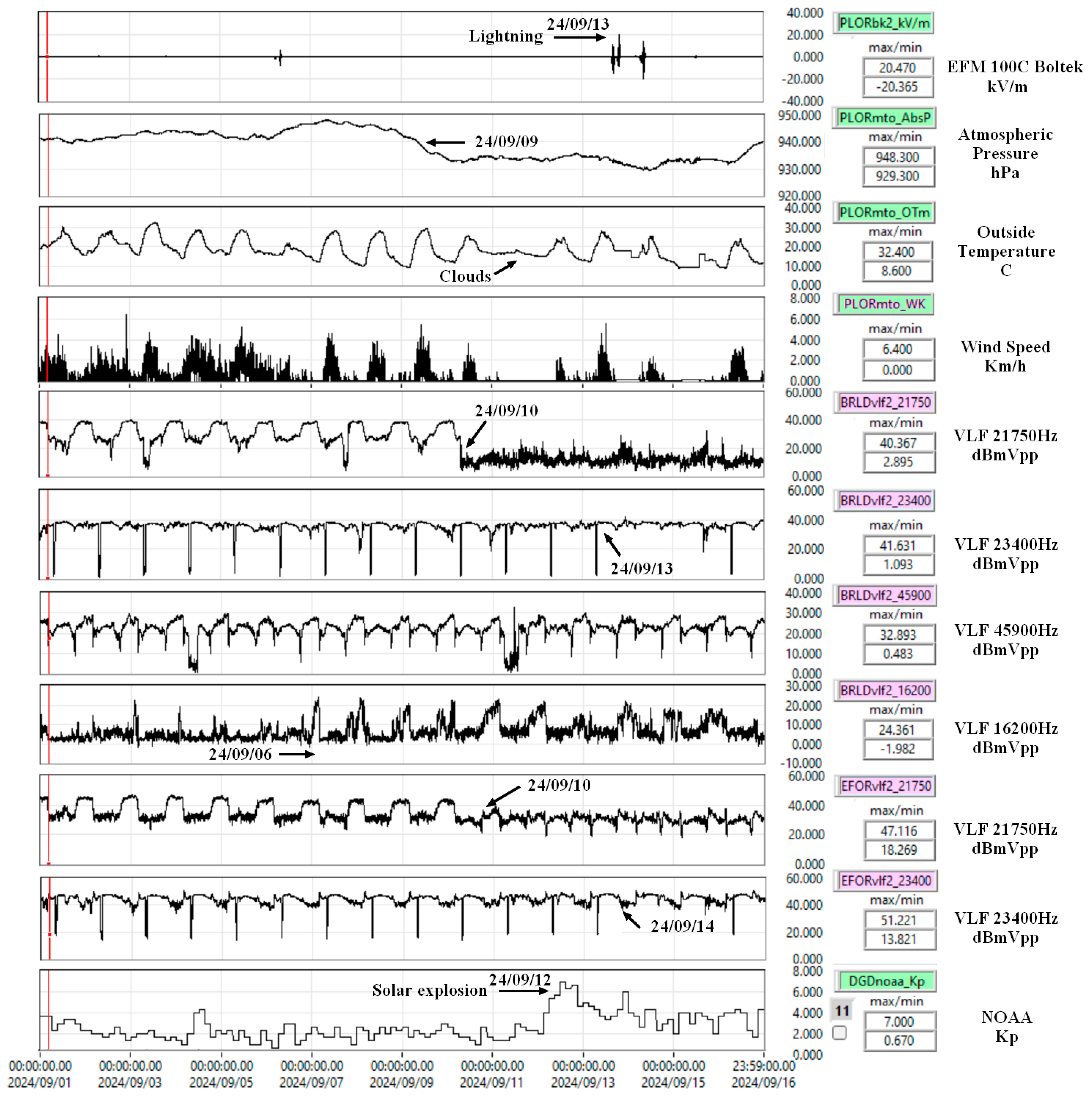
Figure 26.
Strikes over Romania on 16.09.2024, 5 minutes of data.
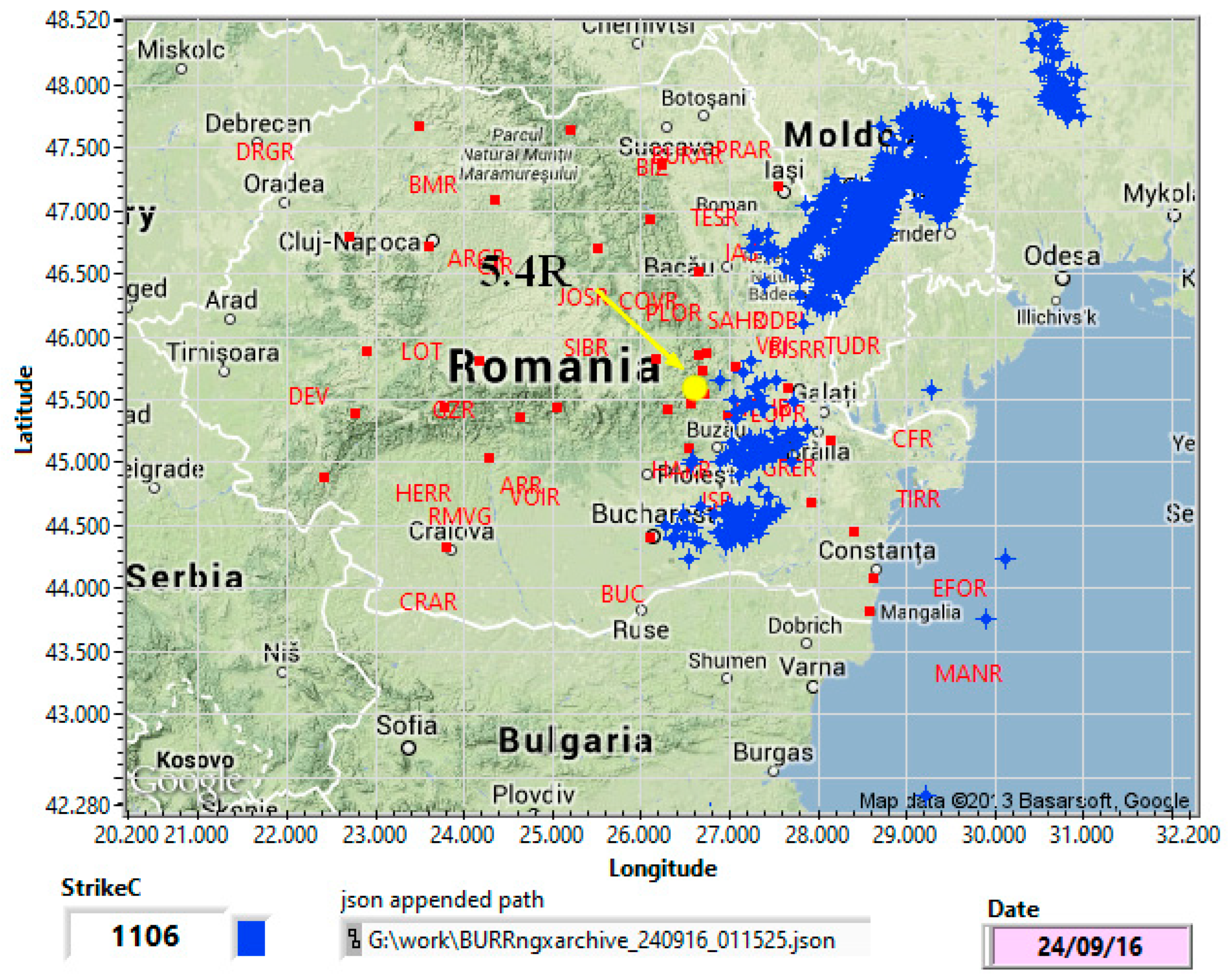
Table 1.
New equipment for gas monitoring of Vrancea area.
| Station | Country | Location | eqp | North | East | Per (sec) |
Description | Start yyyy/mm/dd |
end |
|---|---|---|---|---|---|---|---|---|---|
| VRI2dd | Romania | Vrancioaia | RTM1688 | 45.8657 | 26.7277 | 60 | VRI, RTM 1688-2 radon S/N 519-16 | 2024/10/17 | _ |
| PLORCdd | Romania | Plostina | RTM1688 | 45.8512 | 26.6498 | 60 | PLOR, RTM 1688-2 radon S/N 518-18 | 2024/09/10 | _ |
| VriCH4 | Romania | Vrancioaia | GasCardNG | 45.8657 | 26.7277 | 0.25 | VRI, CH4, Infrared Gas Sensor | 2024/10/25 | _ |
| PlorCH4 | Romania | Plostina | GasCardNG | 45.8512 | 26.6498 | 0.25 | PLOR, CH4, Infrared Gas Sensor | 2024/10/25 | _ |
Table 2.
Radon - Thoron equipment RTM1688-2 produced by SARAD.
| ID | Equipment eqp_RTM1688 | ||||||||||||||||
|---|---|---|---|---|---|---|---|---|---|---|---|---|---|---|---|---|---|
| 1 | Radon | Error | Radon* (fast) | Error | Temp. | relHum | Pres. | Tilt | ROI1 | ROI2 | ROI3 | ROI4 | Ch1 | Ch2 | … | Ch38 | |
| 2 | Bq/m3 | % | Bq/m3 | % | C | % | mbar | _ | cts | cts | cts | cts | cts | cts | … | cts | |
| 3 | %d | %d | %d | %d | %0.1f | %d | %d | %d | %d | %d | %d | %d | %d | %d | … | %d | |
| 4 | RTM1688-2 SARAD, radon thoron | ||||||||||||||||
Table 3.
Radon Radon Scout Plus equipment produced by SARAD.
| ID | Equipment RADONSCOUTp | ||||||
|---|---|---|---|---|---|---|---|
| 1 | Radon | Error | Temp | relHum | Pres | Tilt | ROI1 |
| 2 | Bq/m3 | % | C | % | mbar | _ | cts |
| 3 | %d | %d | %0.1f | %d | %d | %d | %d |
| 4 | radon, Radon, error - Error, temperature in the equipment - Temp, relative humidity in the equipment - relHum, atmospheric pressure - Press, inclination - Tilt, region of interest 1 - ROI1. | ||||||
Table 4.
Radon Radon Scout equipment produced by SARAD.
| ID | Equipment RADONSCOUT | |||||
|---|---|---|---|---|---|---|
| 1 | Radon | Error | Temp | relHum | Tilt | ROI1 |
| 2 | Bq/m3 | % | C | % | _ | cts |
| 3 | %d | %d | %0.1f | %d | %d | %d |
| 4 | radon, Radon, error - Error, temperature in the equipment - Temp, relative humidity in the equipment - relHum, inclination - Tilt, region of interest 1 - ROI1. | |||||
Table 6.
CH4 monitoring equipment.
| ID | Equipment eqp_GasCardNG | |||
|---|---|---|---|---|
| 1 | CH4 | TL | mb | H |
| 2 | % | C | mbar | _ |
| 3 | %0.4f | %0.3f | %0.1f | %d |
| 4 | Chill Card NG Infrared Gas Sensor, CH4 methane, TL lamp temperature, mb air pressure, H humidity | |||
Table 9.
Distance from the epicenter to the monitoring stations.
| Earthquake 5.4R, 45.527600°, 26.352500° | ||
| Station | Latitude, Longitude | Distance (Km) |
| BISRAERd, BISRCO2, Bisoca | 45.548300°, 26.709740° | 28.30 |
| LOPrdd, LOPRCO2, Lopatari | 45.473715°, 26.568721° | 17.84 |
| PANCdd, Panciu | 45.872272°, 27.147726° | 72.76 |
| PLORCdd, Plostina | 45.851396°, 26.649772° | 34.10 |
| VRICdd, VRI2dd, Vrancioia | 45.865695°, 26.727679° | 39.59 |
Table 10.
Vrancea seismicity for earthquakes 2024/08/17 – 2024/09/17.
| N | Time | Ml | Depth | Longitude | Latitude | Mw | PZone |
|---|---|---|---|---|---|---|---|
| yyyy/mm/dd | Richter | Km | Degrees | Degrees | Km | ||
| 1 | 2024/08/17 11:03:54 | 1.1 | 3.4 | 27.833 | 45.506 | 1.67 | 5.2 |
| 2 | 2024/08/17 19:01:29 | 0.6 | 23.3 | 26.5962 | 45.6352 | 1.43 | 4.1 |
| 3 | 2024/08/20 01:12:21 | 2.3 | 71.6 | 26.9662 | 45.7472 | 2.51 | 12 |
| 4 | 2024/08/21 08:02:42 | 0.5 | 5 | 25.1118 | 45.3059 | 1.38 | 3.9 |
| 5 | 2024/08/21 09:46:06 | 1.3 | 17.6 | 25.3323 | 45.2751 | 1.77 | 5.8 |
| 6 | 2024/08/22 17:15:51 | 2.5 | 75.7 | 26.636 | 45.6211 | 2.66 | 13.9 |
| 7 | 2024/08/24 17:12:46 | 3.4 | 144.6 | 26.5364 | 45.6592 | 3.31 | 26.5 |
| 8 | 2024/08/26 22:43:37 | 1.8 | 22.3 | 26.9137 | 45.3975 | 2.03 | 7.4 |
| 9 | 2024/08/27 08:42:29 | 1.5 | 6.9 | 25.7513 | 46.1202 | 1.87 | 6.4 |
| 10 | 2024/08/27 21:25:54 | 1.6 | 29.4 | 27.177 | 45.8624 | 1.92 | 6.7 |
| 11 | 2024/08/28 02:29:02 | 3.4 | 138.2 | 26.5407 | 45.6608 | 3.31 | 26.5 |
| 12 | 2024/08/28 09:16:36 | 1.7 | 5 | 25.7785 | 46.0638 | 1.97 | 7.1 |
| 13 | 2024/08/28 21:22:12 | 2.6 | 89.3 | 26.7991 | 45.867 | 2.73 | 14.9 |
| 14 | 2024/08/29 15:33:22 | 2.6 | 131.6 | 26.5592 | 45.6529 | 2.73 | 14.9 |
| 15 | 2024/08/30 19:12:55 | 3.6 | 73.4 | 26.6597 | 45.7876 | 3.45 | 30.6 |
| 16 | 2024/09/01 11:43:25 | 1.2 | 23.3 | 26.663 | 45.6164 | 1.72 | 5.5 |
| 17 | 2024/09/03 16:50:43 | 3.1 | 120.5 | 26.4318 | 45.4936 | 3.09 | 21.3 |
| 18 | 2024/09/04 21:39:13 | 0.9 | 3 | 27.7967 | 45.5073 | 1.57 | 4.7 |
| 19 | 2024/09/05 02:43:44 | 1.6 | 13.3 | 27.3125 | 45.7081 | 1.92 | 6.7 |
| 20 | 2024/09/05 02:46:09 | 1.7 | 24.1 | 27.2354 | 45.6858 | 1.97 | 7.1 |
| 21 | 2024/09/05 10:32:28 | 1.8 | 7.5 | 25.3004 | 45.3016 | 2.03 | 7.4 |
| 22 | 2024/09/05 12:11:12 | 2.9 | 126.2 | 26.7778 | 45.7678 | 2.95 | 18.5 |
| 23 | 2024/09/05 15:16:04 | 1.1 | 6.3 | 27.8091 | 45.5281 | 1.67 | 5.2 |
| 24 | 2024/09/06 09:55:21 | 1.7 | 8.9 | 25.7295 | 46.0722 | 1.97 | 7.1 |
| 25 | 2024/09/07 21:57:43 | 2.2 | 135.5 | 26.6322 | 45.7638 | 2.44 | 11.2 |
| 26 | 2024/09/07 21:57:43 | 2.2 | 135 | 26.6167 | 45.7585 | 2.44 | 11.2 |
| 27 | 2024/09/09 09:21:33 | 1.5 | 14.2 | 25.6422 | 46.165 | 1.87 | 6.4 |
| 28 | 2024/09/09 13:25:32 | 1.5 | 30.9 | 27.3081 | 45.8753 | 1.87 | 6.4 |
| 29 | 2024/09/10 06:58:56 | 2 | 26.5 | 27.2948 | 45.7896 | 2.13 | 8.2 |
| 30 | 2024/09/10 10:52:16 | 1.4 | 14.9 | 25.3355 | 45.273 | 1.82 | 6.1 |
| 31 | 2024/09/10 23:36:40 | 1.1 | 18 | 26.5345 | 45.4852 | 1.67 | 5.2 |
| 32 | 2024/09/14 15:06:50 | 1.6 | 114.3 | 26.3026 | 45.4852 | 3.24 | 24.6 |
| 33 | 2024/09/15 17:27:59 | 1.7 | 17.9 | 27.8235 | 45.7048 | 1.97 | 7.1 |
| 34 | 2024/09/16 14:40:22 | 5.4 | 126.8 | 26.3525 | 45.5276 | 5.02 | 144.7 |
| 35 | 2024/09/16 16:08:22 | 1 | 12.2 | 27.8053 | 45.5203 | 1.62 | 5 |
| 36 | 2024/09/17 11:33:18 | 1.5 | 8 | 25.2864 | 45.292 | 1.87 | 6.4 |
| 37 | 2024/09/17 18:15:35 | 0.8 | 5 | 25.3469 | 45.3646 | 1.52 | 4.5 |
Disclaimer/Publisher’s Note: The statements, opinions and data contained in all publications are solely those of the individual author(s) and contributor(s) and not of MDPI and/or the editor(s). MDPI and/or the editor(s) disclaim responsibility for any injury to people or property resulting from any ideas, methods, instructions or products referred to in the content. |
© 2024 by the authors. Licensee MDPI, Basel, Switzerland. This article is an open access article distributed under the terms and conditions of the Creative Commons Attribution (CC BY) license (http://creativecommons.org/licenses/by/4.0/).
Copyright: This open access article is published under a Creative Commons CC BY 4.0 license, which permit the free download, distribution, and reuse, provided that the author and preprint are cited in any reuse.


