
Submitted:
15 November 2024
Posted:
18 November 2024
You are already at the latest version
Abstract
Anguilliform swimming is one of the most complex locomotion modes, involving various interacting phenomena, which requires multidisciplinary studies. Eel robots are intended to employ biology principles and exhibit efficient locomotion replicating the natural anguilliform swimming. Such robots are easier to engineer and study than their natural counterparts. Nevertheless, characterizing the robot–environment interaction is complex, demanding computationally expensive fluid dynamics modeling. In this study, we employ machine learning (ML) strategies to discover the temporal evolution of the system, as the data-driven model. Three models were investigated using dynamic mode decomposition (DMD), sparse system identification (SINDy using PySINDy package), and autoencoder neural network (AE NN) as a general function approximator. The models were simulated using MATLAB R2022® to obtain the prediction errors. The results show that the SINDy model presents less error within the regression range, and in particular, performs better within extrapolation. Additionally, the SINDy model has a compact form and can explicitly formulate the coupling phenomena amongst the modes. The identified model, then, was employed to recover the system state data matrix. It is concluded that the proposed model with quadratic terms provides a parsimonious representation of the system dynamics.
Keywords:
swimming robot
; fluid simulation
; aquatic locomotion
; dynamic mode decomposition
; PySINDy
1. Introduction
Snake-like animals exhibit the remarkable ability to navigate through diverse environments without contributing any limbs. This includes moving over complex terrains such as soil, water, slippery surfaces, and narrow spaces. Inspired by these natural capabilities, researchers actively work on the development of bio-inspired robotic systems, designed to replicate the versatile locomotion of snakes [1,2]. These robots are being engineered to traverse and adapt to a wide range of complex and unknown environments like rice paddy [3], ice and unconsolidated sand or snow [4,5], confined spaces [6], and aquatic environments [7]. Swimming snake-like (or eel robots) use body undulations instead of rotary propulsion systems to move forward mimicking animal locomotion. One of the most intricate forms of locomotion is anguilliform swimming which is characterized by its reliance on coordinated body undulations. The locomotion mode is typical of eels and other elongated species. This mode of movement demands a multidisciplinary approach to study, as it involves the integration of multiple interacting phenomena such as fluid dynamics, musculoskeletal mechanics, and neural control. Understanding the biomechanics of anguilliform swimming requires insights from biology, robotics, mathematics, and physics, especially interaction with the surrounding water as the environment. Some eel robots have been developed for mimicking and implementing efficient biology principles in robots, or for testing hypotheses regarding natural swimmers.
Soft robots are extensively studied for aquatic navigation tasks [8,9]. Soft robots can replicate some animal gesticulation due to their structural compliance and versatile movement like bending, twisting, and extension [10]. As noted in [11], conceivable gaits for elongated soft robots include crawling (two-anchor, peristaltic, and serpentine types), and anguilliform swimming. Various swimming soft robots have been proposed to replicate the locomotion and anatomy of eels [11,12,13,14]. An eel robot using fiber-reinforced soft actuators is proposed in [13]. In [15], a swimming eel robot was introduced, and its interaction with the water as the environment was studied using numerical simulation data and modal decomposition. As locomotion involves complex wave propagation along the body, characterization of the robot-environment interaction modes helps to gain insight into locomotion physics. Characterization of the hydrodynamic model with explicit mathematical equations would provide interpretable models, which may help to comprehend and optimize the robot locomotion.
In many real-world problems, including the hydrodynamics of anguilliform swimmers, the direct formulation of the dynamical model is extremely complicated. To model complex systems, a newer approach known as data-driven modeling relies on data rather than the foundation of explicit theoretical models. In this approach, large datasets are used to identify patterns, relationships, and behaviors within a system, leveraging techniques such as machine learning (ML), statistical analysis, and artificial intelligence (AI). Unlike traditional modeling, which depends on fundamental equations and boundary assumptions, data-driven models adapt and refine themselves based on the input data. A classic data-driven method to break down complex behavior of dynamical systems into oscillatory modes is dynamic mode decomposition (DMD). Especially when the system dynamics are governed by linear components or the nonlinearity can be approximated by linear modes, the standard DMD represents a linear operator that maps one state vector of the system to the next over time. DMD was first introduced in the fluid dynamics community [16], and has received great research interest, extensions, and applications in different fields [17].
In cases where dealing with systems in which the underlying physical or mathematical principles are unknown or too complex to model, nonlinear data-driven techniques are employed to estimate or fit a parsimonious model to the measured data. This makes them highly useful in fields such as engineering, biology, economics, and climate science. A cutting-edge data-driven technique to identify the governing equations of dynamical systems directly from observed data is sparse identification of nonlinear dynamics (SINDy [18,19,20]). It is particularly effective when dealing with nonlinear systems, where traditional modeling approaches may struggle. The power of SINDy is in the identification of systems that can be described by a small set of dominant terms, while most remaining terms of a library of functions contribute little to the dynamics. SINDy uses sparsity-promoting techniques such as L1 regularization to select only the most important terms from the function library (a large candidate set of possible functions). This approach helps to construct the simplest mathematical model that explains the system’s dynamics.
The inputs to the SINDy algorithms include a data matrix of system state measurements over time, and a library of candidate functions (including polynomial, trigonometric, or other basis functions). The algorithm identifies the terms essential for describing the state update from one step to the next using a sparse regression process. This empowers SINDy to discover interpretable and compact models, which is very useful in fields like fluid dynamics, neuroscience, and mechanical systems, where extracting meaningful equations from data is crucial for understanding complex behavior. In comparison with neural networks (NN) an advantage of SINDy is the presence of interpretable models, which highlight insights into the underlying physics or biology driving the system. The balancing between simplicity with accuracy, which is provided by adjusting an optimization factor, is a powerful tool for understanding and predicting the behavior of nonlinear systems.
In this paper, we extend the previous study on robot-environment interaction mode analysis [15], investigating data-driven modeling of the temporal modes. First, in Section 2.1, the data collection is introduced. In Section 2.2, the methods used to approximate the time evolution of the modes are introduced. The methods include a linear model regression using a DMD technique, the SINDy model, and an autoencoder neural network (AE NN) model. The resulting regression function is given in Section 3.1. Simulation results for comparison of the SINDy model with the others are given in Section 3.2. Section 3.3 presents simulation results for the reconstruction of the data based on the proposed model. Finally, in Section 4, the results are discussed followed by the conclusion.
2. Materials and Methods
2.1. Data Preparation
The first step in the data-driven modeling method involves systematically collecting reliable data to serve as the substance for further analysis. This initial data, essential for constructing an accurate and representative model, was gathered through a combination of practical experiments and computational simulations. Specifically, to capture the system dynamics, key kinematic parameters—including the required activation frequency, the robot's forward velocity, and the amplitude of undulation—were derived empirically. Given the complex, largely unknown nature of the system’s dynamics, it was impossible to predefine these parameters accurately without conducting exploratory experiments. Figure 1 shows the robot’s swimming through a water tank. The robot structure and model are shown in Figure 2. Within the experiments, various parameters were manually varied adjusted, and observed until the working values for achieving a desirable swimming motion were identified.
With these empirically determined parameters in hand, we built a detailed model of the robotic system using COMSOL Multiphysics® 6.1. In this software model, a virtual representation of the robot—the ‘digital twin’—was developed as in Figure 2c. This digital twin enabled us to simulate the velocity field around the robot, reflecting the dynamics observed in real-world experiments. The digital twin was calibrated with experimentally measured parameters, including the actuation pattern, frequency, and the robot’s forward speed. The robot's forward speed, measured experimentally, defined the fluid inlet conditions within the digital twin simulation environment, while the actuation pattern and frequency were modeled as the driving force inputs that replicate the robot’s actual movement. These inputs allow the digital twin to simulate realistic conditions, making it possible to analyze the system's behavior.
By integrating experimentally measured parameters into the digital twin, we ensured that the model accurately reflected the physical system, providing a reliable basis for further analysis. The robot is a soft-bodied structure designed to perform anguilliform locomotion, where the entire body contributes to the generation of wave-like movements. This type of locomotion is efficient for navigation in water, especially in environments where eels and similar creatures thrive. The structure and design prioritizes flexibility and adaptability in water, with a segmented, elongated body allowing for bending motions similar to those of a natural eel. The structure contains six actuated segments, where each segment contains two contraction-type soft actuators (McKibben artificial muscles) on each side. The actuators contract when pneumatically pressurized.
The robot's movement is obtained by a monotonic segmental bending realized by square waveforms activating the lateral pneumatic muscles. Each actuated segment bends laterally when the actuator pair at the side is contracted. An electro-pneumatic controller makes a monotonic sequence like this: Turn segment 1 to the right (1R) and segment 4 to the left (4L) by turning on 1R-4L, then 2R-5L, 3R-6L, 4R-1L, 5R-2L, 6R-3L, 6R-1L, and again 1R-4L and so on. The period, T, is the time for a full cycle so that any actuator will be activated for T/6 in a cycle.
2.2. Decomposition and Regression Methods
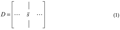
A finite element FE model was used to simulate the hydrodynamic problem and calculate the normal velocity field as the time history of the system state, which is arranged as a vector . The state vectors are assembled as time snapshots of the data matrix, , as follows
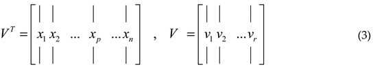
The first step of the proposed method involves the decomposition of the data matrix based on singular value decomposition (SVD) and order reduction,

The matrices, , , and are obtained by r-order truncated SVD. In this context, the superscript, T, shows the matrix transpose. One interesting property of SVD is that it separates the spatial and temporal modes, so that only the VT is varied in time. Therefore, it would be interesting to search for a model for the temporal part to estimate the system dynamics. The matrix, V, has vi i = 1..r vectors as its columns, and k = 1..n vectors as its rows. Note that xk, columns of VT, are known as the time snapshots at t = kΔT k = 1...n where ΔT is the sampling time.
The objective is to discover or fit a function, , so that

The equation is to be determined using optimization over the training data, k = 1...p p < n, and predicts the next time step of the state based on the current snapshot. Various approaches can be employed for this purpose.
2.2.1. DMD Approach
For approximating a linear model, following the DMD method, the function is written with a matrix A as follows

Suppose matrices X and X+ are constructed as
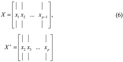
It has been proven that an L2-Norm best-fit solution, A, satisfies X+ = AX (In the standard DMD, due to large matrix sizes, a reduced-size matrix is measured). The solution of (5) is readily calculated based on the eigendecomposition as

where Λ is the eigenvector matrix of X+ XT, Ω = diag{ωi} is the matrix of the corresponding eigenvalues, ωi.
The update function obtained from the DMD method will be:

2.2.2. SINDy Approach
Real physical systems, despite nonlinearity, have relatively few active terms in their dynamics, (4). Based on this assumption, SINDy supposes the model in the form of

where Θ is a library of l test functions, and is the sparse matrix of coefficients. In this work, the PySINDy algorithm finds a sparse matrix of coefficients that relates a library of candidate functions to the matrix of time derivatives, , as in

In this context, the time derivative is approximated using the finite difference (FD) method, given the sampling time, ΔT, using
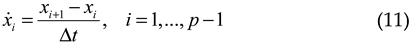
This formulation follows the forward Euler method that works well for high-resolution time steps and has the advantages of simplicity and real-time applicability. Considering a sparsity regularization parameter, ε, the matrix Ξ is found by solving the optimization problem:

The optimization problem, in this work, is solved with PySINDy. The Python package solves a least square problem to minimize , then sets entries to zero, and the iteration is continued. We choose a sequentially thresholded least squares (STLSQ) optimizer with the threshold ε = 0.95 (That means coefficients smaller than 0.95 are set to zero). The STLSQ algorithm in SINDy [18], instead of an L1-minimization in (12), enforces sparsity in the coefficient matrix and mitigates measurement noise impact. In this work, the polynomial feature library of degree two is used. Finally, the discrete update equation can be represented as

PySINDy returns the equation explicitly, which can be coded directly, e.g. as a function within MATLAB® R2022b.
2.2.3. AE NN Approach
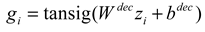
In the AE NN, a nonlinear NN model, f(xi) = NN(xi), is trained by minimizing a mean square error (MSE) of the loss function. A feedforward NN is constructed and trained using a scaled conjugate gradient algorithm, trainscg, of MATLAB® R2022b. The nonlinearity is due to the activation function of the hidden layer, which is chosen to be a hyperbolic tangent sigmoid function. The AE NN is mathematically expressed with the encoder and decoder formulas. The encoder with weight matrix Wenc and bias vector benc maps inputs xi to the latent variables hi with

The bottleneck layer is represented with a weight matrix, Wneck, and bias, bneck, as a linear function zi = Wneckhi + bneck. The decoder with weight matrix, Wdec, and bias vector, bdec, decodes the latent variables, zi, as
A linear output layer with eight matrix, Wout, and bias vector , bout, returns the next data snapshot with:

The training involves estimation of the weights and biases entries based on optimization of the loss function, given as
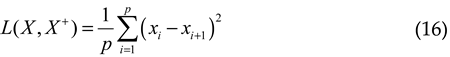
The update function can be expressed as

3. Results
3.1. Regression Function
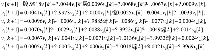
The regression problem estimates a function for the approximation (4). A powerful Python library designed to discover governing equations from time-series data, PySINDy, was used to measure the SINDy model. Within the code, the optimizer parameter was set to STQL with a threshold value of 0.95 to control the minimum coefficient magnitude considered in the model. Additionally, a polynomial with a degree of two and no bias was set as the feature library, and a first-degree FD was defined as the derivative approximator within the Python code. The result is as follows:
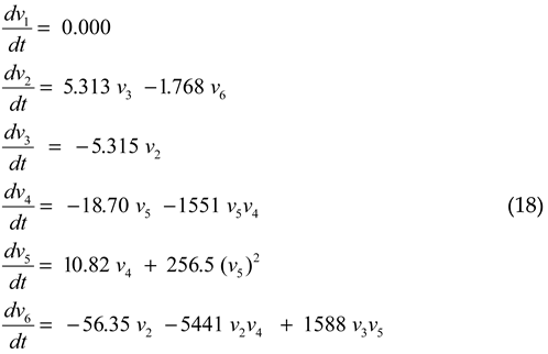
This ordinary differential equation describes the v1 to v6 modes of the system, with r=3 in (3). Important details can be inferred from each equation in (18). The first equation indicates that the first mode, v1, remains unchanged through the system evolution. Secondly, the system of equations shows the coupling between the modes. The second and third equations represent a subsystem with oscillatory behavior between modes 2 and 3. This subsystem is linear, in form, and can be attributed to the traveling wave. However, as mode 6 (v6 in the second equation) is coupled to the subsystem, it can induce exotic oscillations. The nonlinear terms, the quadratic terms and the cross-products of the modes are responsible for the complex dynamics of the system. Note that, with sampling time Δt = 0.001(s) in (11), the discrete form of (18) can be represented as
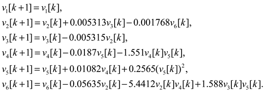
Note that the updating equation, corresponding (13), is as

It is worth to mention the related equation (8), obtained with the DMD technique. The numerical model is given as
Note that DMD represents the best possible linear model fitted to the data. The success of such fitting relies on system physics. A comparison of the equations shows that the SINDy method results in a compact and understandable model. The AE NN model contains an even more complex system of equations. Selecting 12 neurons in the encoder and decoder, and 3 neurons in the bottleneck, in (17), Wout is 6 by 12, Wdec is 12 by 3, Wneck is 3 by 12, and Wenc is a 12 by 6 matrix.
3.2. Simulation of the Regression Methods
The methods described in the previous section were implemented in MATLAB® R2022 using the data matrix, X+, for calculation of the function predicting the next time-step described as in (4). The simulation results of the estimated functions xi+1 ≈ f(xi) and original data, X+, are shown in Figure 3, for the DMD model, Figure 4, for the SINDy identified model, and Figure 5, for an AE NN as an arbitrary nonlinear approximator. The errors, which in this case are the difference between the original and predicted data are shown in Figures 3b, 4b, and 5b. The first visual check shows that the SINDy model has fewer errors than the DMD model. As DMD provides a linear model, it would be interesting to compare the results with a universal nonlinear approximator. A comparison of the Figure 4 and Figure 5 shows the AE NN also exhibits more errors. Another advantage of the SINDy model over NN methods is the parsimonious explicit equations provided by the method.
One useful property of the data-driven models would be the capability of extrapolation and prediction over the training horizon. Although the interpolation abilities within the X+ range, shown in Figures 3a, 4a, and 4a suggest a desirable match, it would be interesting to observe the result of the entire data range, VT. In other words, the simulation can be extended to estimate xp to xn using the estimated functions to calculate the errors. Figure 6 shows the errors, while the cyan line represents a typical band for visual comparison of the errors. Figure 6a represents the DMD model results, suggesting rapid error growth during the extrapolation. Figure 6b represents the results for the SINDy model. Finally, Figure 6c shows that the AE NN presents big error values, making the model unreliable for prediction purposes. The comparison shows another advantage of the SINDy model: presenting less extrapolation error. The cyan band highlights the range of error, where during 40 ms the SINDy is still within the band.
3.3. SINDy Data-Reconstruction
Data reconstruction refers to the simulating of a numerical model to recreate or approximate the original dataset from reduced or transformed data. In the context of data-driven modeling like SINDy or other approaches, reconstruction involves using the learned model (the set of identified equations) to predict or simulate the system's behavior over time. The reconstructed data is then compared with the original data to evaluate how well the model captures the system dynamics. The comparison is best realized by visualization of the data in image form, particularly for high-dimensional data where simple numerical comparison may be insufficient to capture complex patterns or trends. For this aim, the original data used to identify the update function and the corresponding data obtained from the simulation of the identified model are shown in Figure 7. For comparison, a zoomed view is also provided in Figure 8, exhibiting the error matrix in Figure 8c which indicates that the error grows in the extrapolation range.
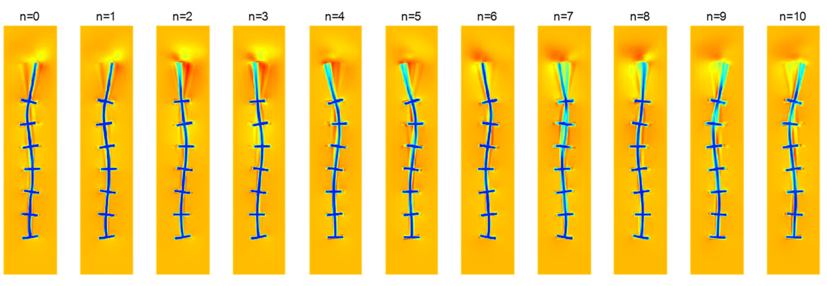
The vectorized data is readily rearranged to the original spatial size to have an interpretable representation of the robot-environment states. The image representation of one full cycle in 10 steps is shown in Figure 9. Note that the images represent the original data time evolution for the last period. Figure 10 represents the corresponding state data reconstructed using the SINDy model. Accurate reconstruction indicates that the model successfully captured the dominant patterns and relationships within the data. The results suggest that the model can be used as a surrogate model of the robot–environment system. Such models are useful in predicting the system states with rapid measurements (as required, e.g., in real-time control applications).
4. Discussion
Aquatic locomotion involves a complex interaction between the swimmer's body and the environment, which is described with incompressible fluid dynamics equations and relations. Modeling fluid dynamics problems is generally involved. In particular, the fluid interacting with the swimmer’s body involves complicated high-dimensional equations needing huge computation power for simulation. Such numerical models are not practically useful in real-time applications. Moreover, in computational methods, the model is not comprehendible by itself, and commonly the simulation results or the outputs, normally in graphic presentation, are studied instead of the high-dimensional mathematical model. Referring to the specific problem of anguilliform locomotion, the swimming robot possesses complicated dynamics and exhibits exotic temporal modes that are not expressed coherently in the normal coordinates. This paper tries to evaluate the ability of well-established data-driven methods to identify possible interplay between the modes. The results of this study suggest that a compact quadratic model obtained from truncated SVD decomposition and SINDy can describe the states of the system, including the velocity field of the fluid domain and the robot's posture. The results showed that a pure linear model obtained from DMD has more errors concerning the SINDy model. Moreover, the SINDy model shows a better ability to predict future steps, within extrapolation. The comparison indicates that the system dynamics have quadratic performance that a linear approximator could not fully describe. The next question about the performance of the proposed model was can the advantage be merely for adding a nonlinearity? Could an inclusion of a random nonlinearity term do as well? The comparison with an AE NN model, as a general nonlinear approximator, shows that SINDy model still outperforms in terms of prediction error, with an additional advantage of parsimony due to explicit and compact model representation. The reconstruction result confirms the ability of the model to predict the system behavior. The ability of the SINDy model to predict future states and extrapolation can be used for further studies such as observer and feedback control design. A similar study can be proposed to obtain the fluid states of a filmed swimmer.
5. Conclusions
Anguilliform locomotion contains complicated dynamics due to the complex interactions between the fluid and the swimmer. The performance of man-made machines or bioinspired robots mimicking anguilliform locomotion is not still comparable with biological counterparts. This study focused on data-driven modeling of the temporal behavior of a swimming robot based on a truncated SVD representation of simulation data. Three models based on DMD, SINDy, and NN were examined. The simulation and computation results show that the SINDy model identifies a compact model that can be used for the prediction of hydrodynamic behavior, with less regression and extrapolation errors concerning the other methods. The model was used for the reconstruction of the snapshots of the training data. The results show the ability of the data reconstruction, in particular within the regression range. Furthermore, the explicit model obtained by SINDy explains the coupling between the modes. The mathematical equation shows that two modes contribute to the anguilliform undulation, while the other modes affect the undulation modes with a nonlinearity influence. The conclusion suggests that the system contains quadratic nonlinearities revealing rich dynamics that may not be reflected by a linear model.
Author Contributions
Conceptualization, M.S. and H.W.; methodology, M.S.; software, M.S.; validation, M.S. and H.W.; formal analysis, M.S.; investigation, M.S. and H.W.; resources, M.S. and H.W.; data curation, M.S. and H.W.; writing—original draft preparation, M.S.; writing—review and editing, H.W.; visualization, M.S.; supervision, H.W.; project administration, M.S. and H.W.; funding acquisition, H.W. All authors have read and agreed to the published version of the manuscript.
Funding
M.S.'s work has been supported by a grant from the County of Thuringia (Landesgraduiertenstipendium des Freistaats Thüringen).
Conflicts of Interest
The authors declare no conflicts of interest.
References
- Cortez, R.; Sandoval-Chileño, M.A.; Lozada-Castillo, N.; Luviano-Juárez, A. Snake Robot with Motion Based on Shape Memory Alloy Spring-Shaped Actuators. Biomimetics 2024, 9, 180. [Google Scholar] [CrossRef] [PubMed]
- Seyidoğlu, B.; Rafsanjani, A. A textile origami snake robot for rectilinear locomotion. Device 2024, 2. [Google Scholar] [CrossRef]
- Aoki, T.; Inada, S.; Shimizu, D. Development of a Snake Robot to Weed in Rice Paddy Field and Trial of Field Test. In Proceedings of the 2024 IEEE/SICE International Symposium on System Integration (SII); 2024; pp. 1537–1542. [Google Scholar]
- Thakker, R.; Paton, M.; Strub, M.P.; Swan, M.; Daddi, G.; Royce, R.; Tosi, P.; Gildner, M.; Vaquero, T.; Veismann, M. EELS: Towards Autonomous Mobility in Extreme Terrain with a Versatile Snake Robot with Resilience to Exteroception Failures. In Proceedings of the 2023 IEEE/RSJ International Conference on Intelligent Robots and Systems (IROS); 2023; pp. 9886–9893. [Google Scholar]
- Georgiev, N.; Pailevanian, T.; Ambrose, E.; Archanian, A.; Melikyan, H.; de Mola Lemu, D.L.; Gildner, M. EELS: A Modular Snake-like Robot Featuring Active Skin Propulsion, Designed for Extreme Icy Terrains. In Proceedings of the 2024 IEEE Aerospace Conference; 2024; pp. 1–15. [Google Scholar]
- Virgala, I.; Varga, M.; Sinčák, P.J.; Merva, T.; Mykhailyshyn, R.; Kelemen, M. Mathematical framework for snake robot motion in a confined space. Applied Mathematical Modelling 2024, 132, 22–40. [Google Scholar] [CrossRef]
- Bianchi, G.; Lanzetti, L.; Mariana, D.; Cinquemani, S. Bioinspired Design and Experimental Validation of an Aquatic Snake Robot. Biomimetics 2024, 9, 87. [Google Scholar] [CrossRef] [PubMed]
- Ng, C.S.X.; Tan, M.W.M.; Xu, C.; Yang, Z.; Lee, P.S.; Lum, G.Z. Locomotion of miniature soft robots. Advanced Materials 2021, 33, 2003558. [Google Scholar] [CrossRef] [PubMed]
- Yu, Q.; Gravish, N. Multimodal Locomotion in a Soft Robot Through Hierarchical Actuation. Soft Robotics 2024, 11, 21–31. [Google Scholar] [CrossRef] [PubMed]
- Yao, D.R.; Kim, I.; Yin, S.; Gao, W. Multimodal soft robotic actuation and locomotion. Advanced Materials 2024, 2308829. [Google Scholar] [CrossRef] [PubMed]
- Chen, Y.; Wang, T.; Wu, C.; Wang, X. Design, control, and experiments of a fluidic soft robotic eel. Smart Materials and Structures 2021, 30, 065001. [Google Scholar] [CrossRef]
- Nguyen, D.Q. Evaluation on swimming efficiency of an eel-inspired soft robot with partially damaged body. In Proceedings of the 2021 IEEE 4th International Conference on Soft Robotics (RoboSoft); 2021; pp. 289–294. [Google Scholar]
- Dang, R.; Gong, H.; Wang, Y.; Huang, T.; Shi, Z.; Zhang, X.; Wu, Y.; Sun, Y.; Qi, P. Bionic body wave control for an eel-like robot based on segmented soft actuator array. In Proceedings of the 2021 40th Chinese Control Conference (CCC); 2021; pp. 4261–4266. [Google Scholar]
- Cervera-Torralba, J.; Kang, Y.; Khan, E.M.; Adibnazari, I.; Tolley, M.T. Lost-Core Injection Molding of Fluidic Elastomer Actuators for the Fabrication of a Modular Eel-Inspired Soft Robot. In Proceedings of the 2024 IEEE 7th International Conference on Soft Robotics (RoboSoft); 2024; pp. 971–976. [Google Scholar]
- Sayahkarajy, M.; Witte, H. Analysis of Robot–Environment Interaction Modes in Anguilliform Locomotion of a New Soft Eel Robot. In Proceedings of the Actuators; 2024; p. 406. [Google Scholar]
- Schmid, P.J. Dynamic mode decomposition of numerical and experimental data. Journal of fluid mechanics 2010, 656, 5–28. [Google Scholar] [CrossRef]
- Schmid, P.J.J.A.R.o.F.M. Dynamic mode decomposition and its variants. 2022, 54, 225–254. [Google Scholar] [CrossRef]
- Brunton, S.L.; Proctor, J.L.; Kutz, J.N. Discovering governing equations from data by sparse identification of nonlinear dynamical systems. Proceedings of the national academy of sciences 2016, 113, 3932–3937. [Google Scholar] [CrossRef] [PubMed]
- de Silva, B.M.; Champion, K.; Quade, M.; Loiseau, J.-C.; Kutz, J.N.; Brunton, S.L. Pysindy: a python package for the sparse identification of nonlinear dynamics from data. arXiv preprint arXiv:.08424 2020. [Google Scholar] [CrossRef]
- Kaptanoglu, A.A.; de Silva, B.M.; Fasel, U.; Kaheman, K.; Goldschmidt, A.J.; Callaham, J.L.; Delahunt, C.B.; Nicolaou, Z.G.; Champion, K.; Loiseau, J.-C. PySINDy: A comprehensive Python package for robust sparse system identification. arXiv preprint arXiv:.08481 2021. [Google Scholar] [CrossRef]
Figure 1.
Actual swimming of the robot.
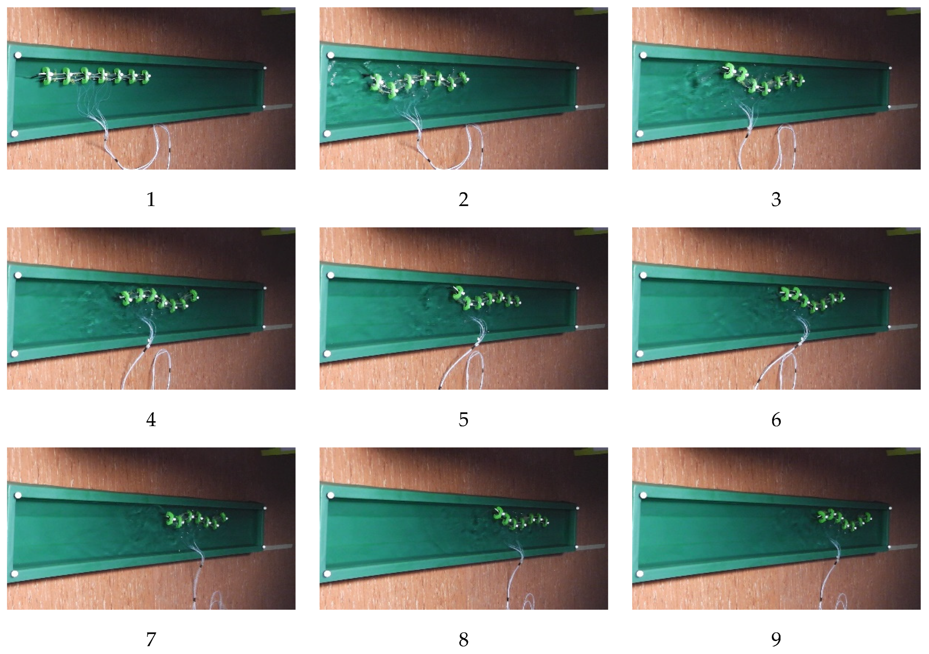
Figure 2.
Structure and model of the system: (a) 3D view and main dimensions; (b) 2D view and arrangement of the contraction actuators; (c) the simulation model.
Figure 2.
Structure and model of the system: (a) 3D view and main dimensions; (b) 2D view and arrangement of the contraction actuators; (c) the simulation model.
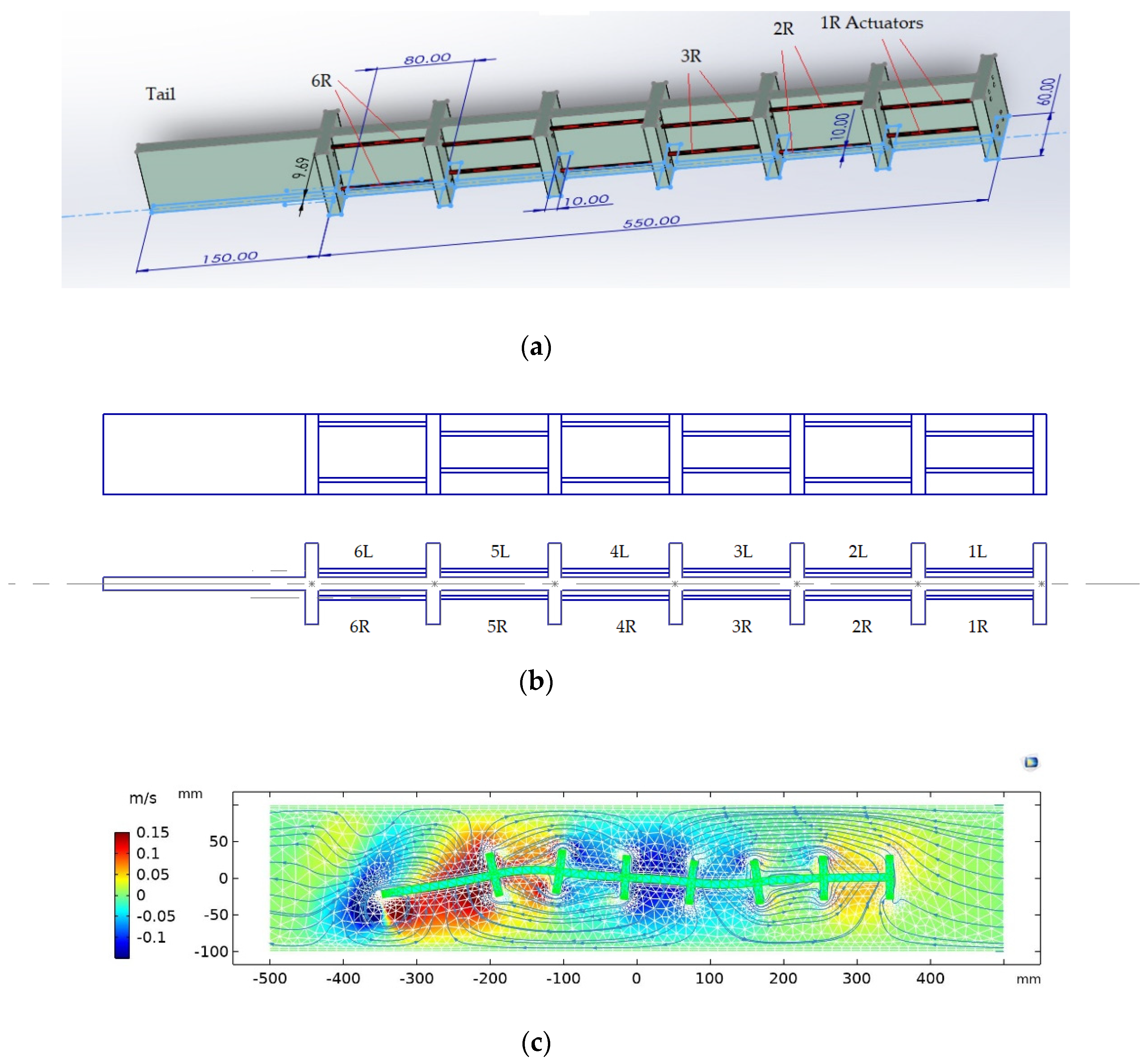
Figure 3.
Simulation results with the linear model: (a) The DMD prediction and original data; (b) the error values.
Figure 3.
Simulation results with the linear model: (a) The DMD prediction and original data; (b) the error values.
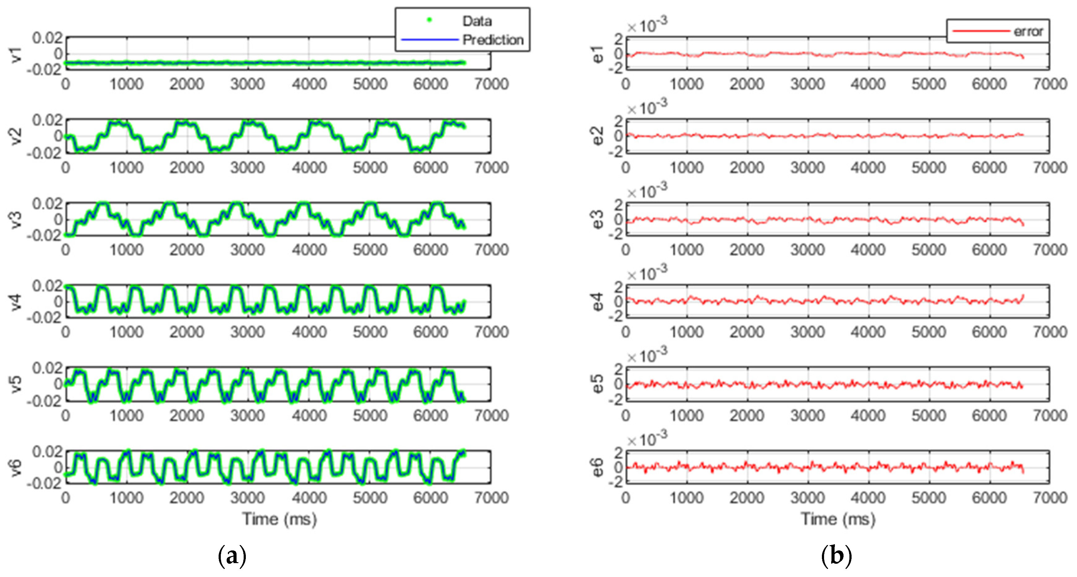
Figure 4.
Simulation results with the SINDy model: (a) The SINDy prediction and original data, X+ ; (b) the error values.
Figure 4.
Simulation results with the SINDy model: (a) The SINDy prediction and original data, X+ ; (b) the error values.
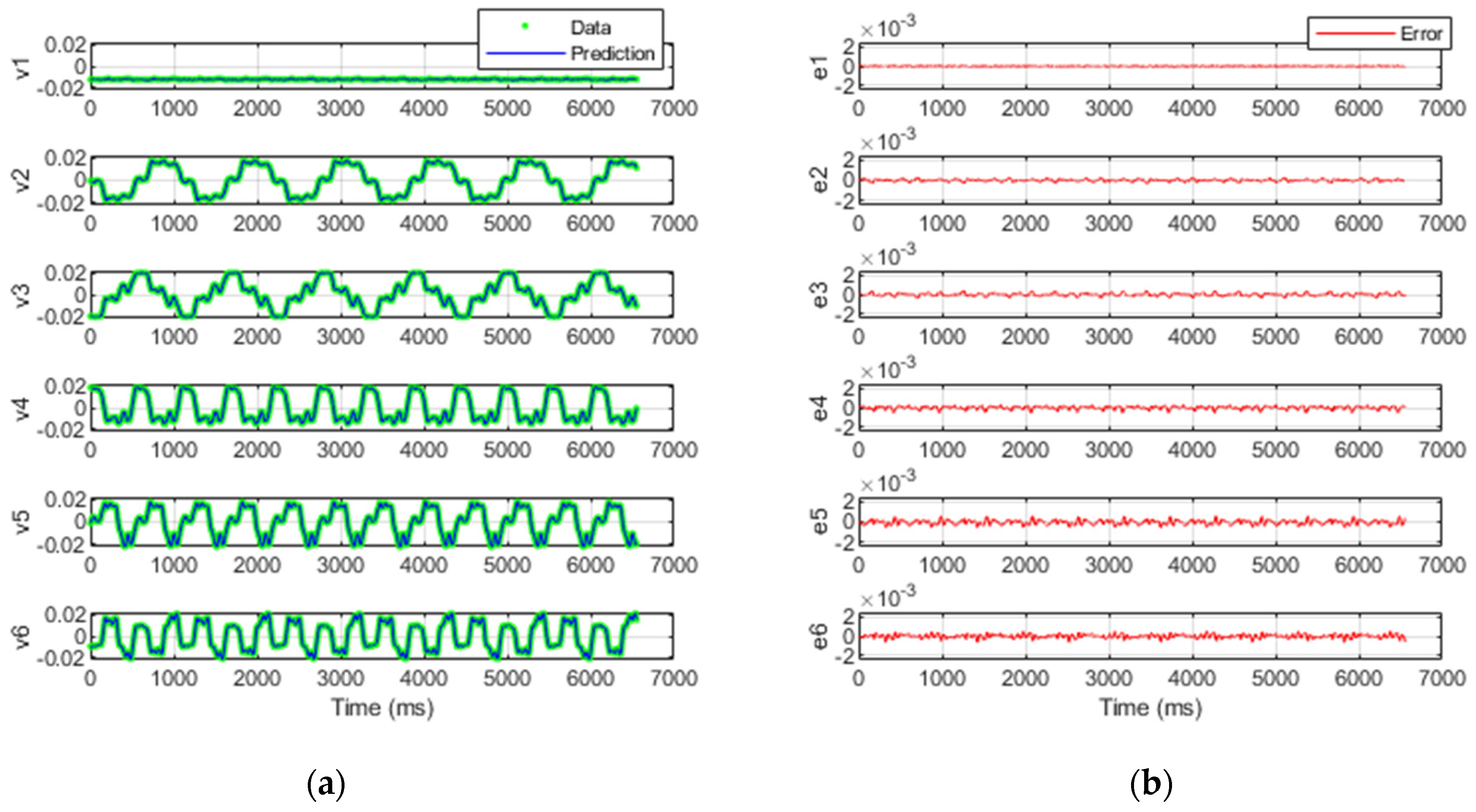
Figure 5.
Simulation results with the AE NN nonlinear model: (a) The AE NN prediction and original data; (b) the error values.
Figure 5.
Simulation results with the AE NN nonlinear model: (a) The AE NN prediction and original data; (b) the error values.
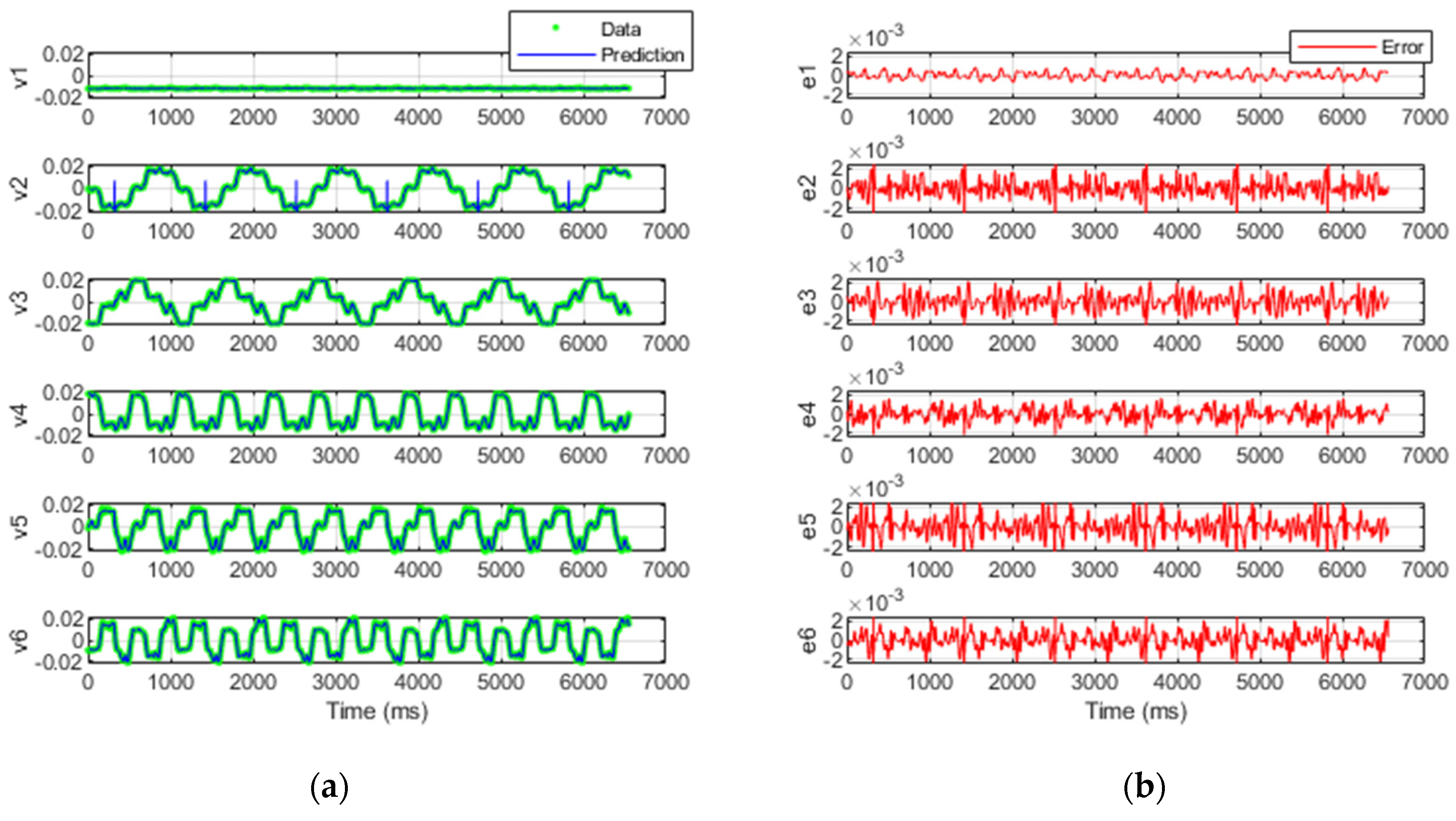
Figure 6.
Comparison of the prediction errors considering extrapolated data: (a) The DMD prediction; (b) the SINDy model results; (c) an AE NN.
Figure 6.
Comparison of the prediction errors considering extrapolated data: (a) The DMD prediction; (b) the SINDy model results; (c) an AE NN.
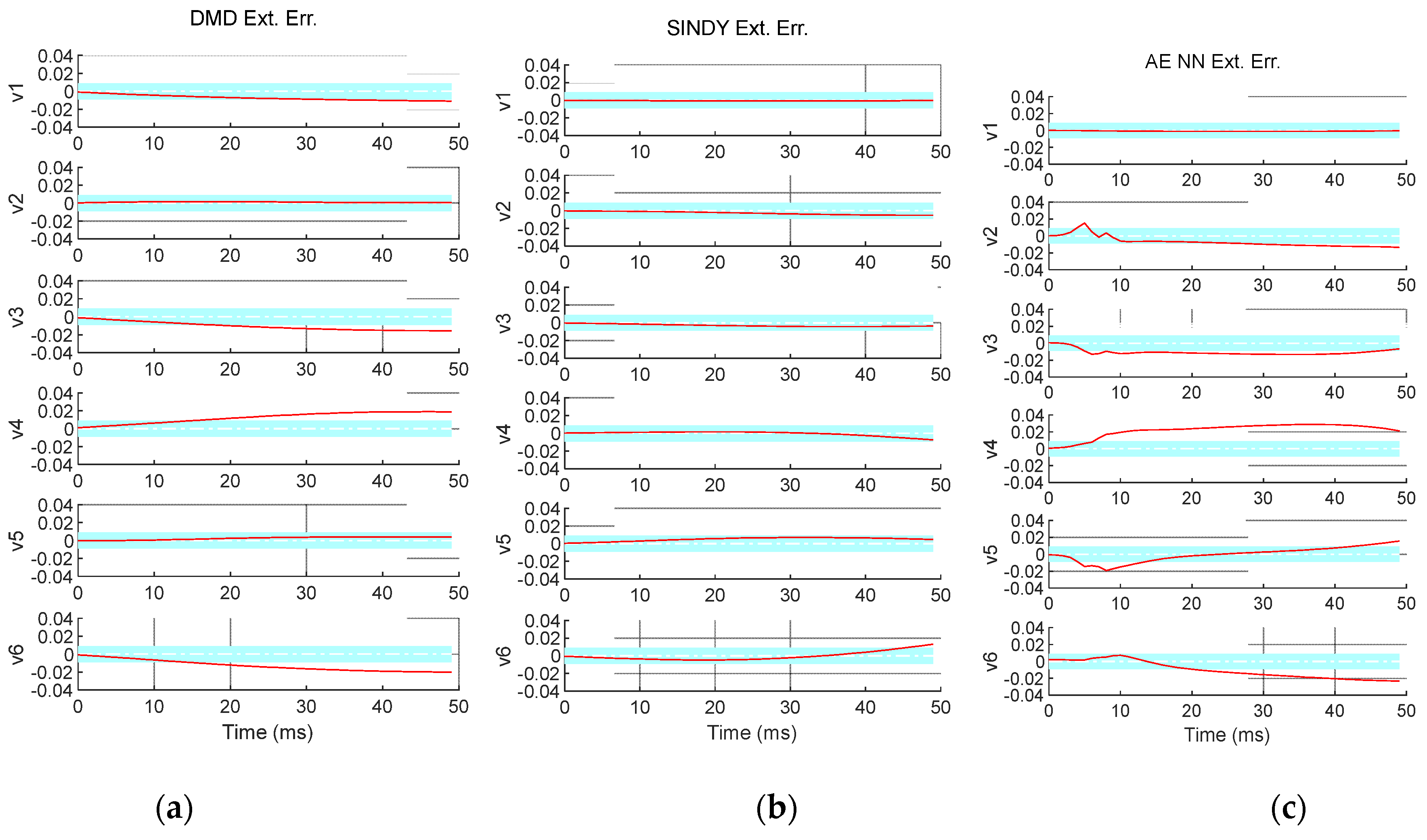
Figure 7.
Visualized data matrices: (a) The original data, VT; (b) the SINDy-reconstructed data.
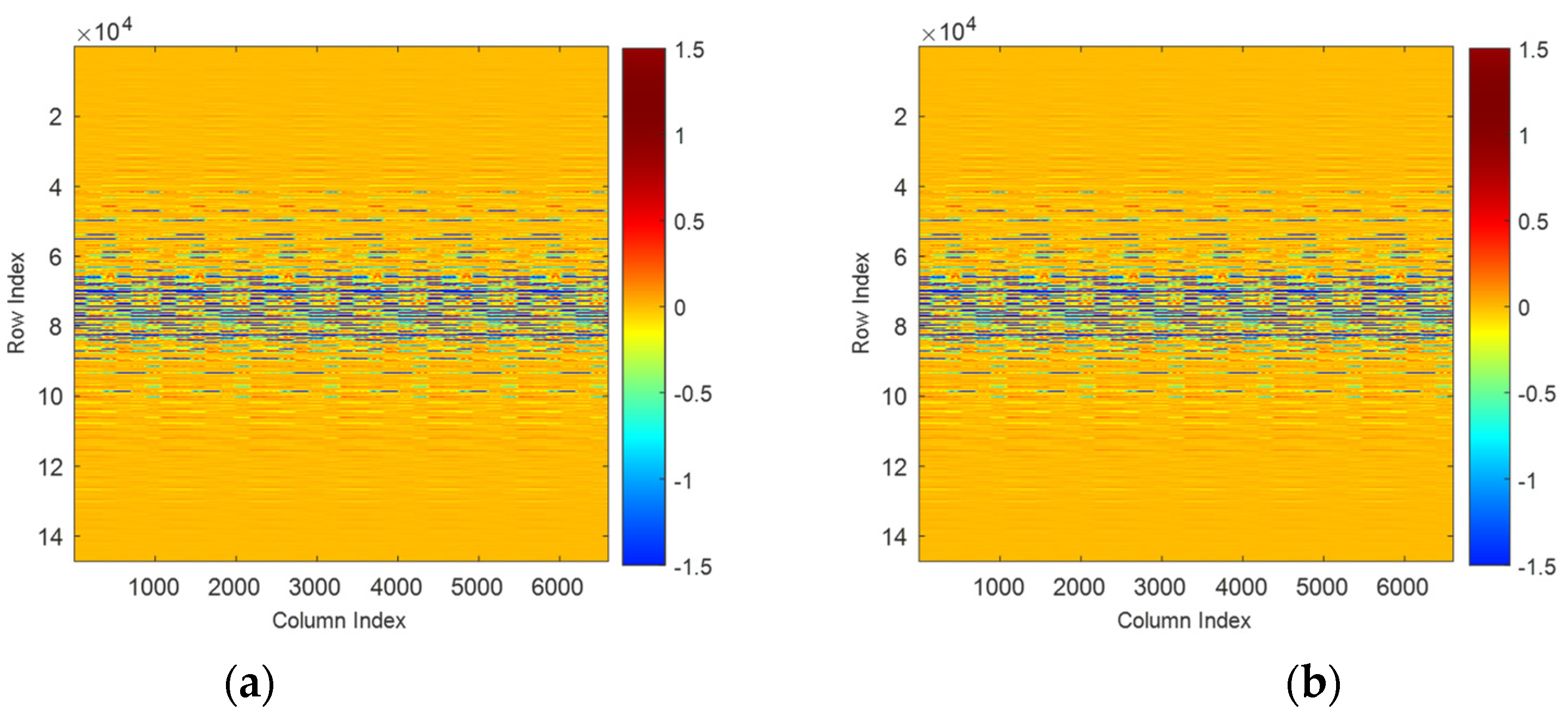
Figure 8.
Visualization of the reconstruction errors considering extrapolated data: (a) The original data; (b) the SINDy model results; (c) the error (difference).
Figure 8.
Visualization of the reconstruction errors considering extrapolated data: (a) The original data; (b) the SINDy model results; (c) the error (difference).
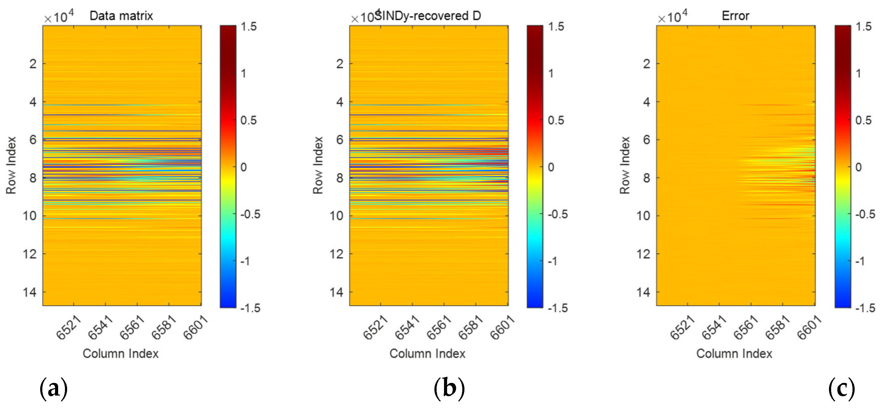
Figure 9.
Time-evolution of the robot–environment states, , of the original data matrix D in one period. The numbers, n, refer to the time, nT/10, where T is the period.
Figure 9.
Time-evolution of the robot–environment states, , of the original data matrix D in one period. The numbers, n, refer to the time, nT/10, where T is the period.
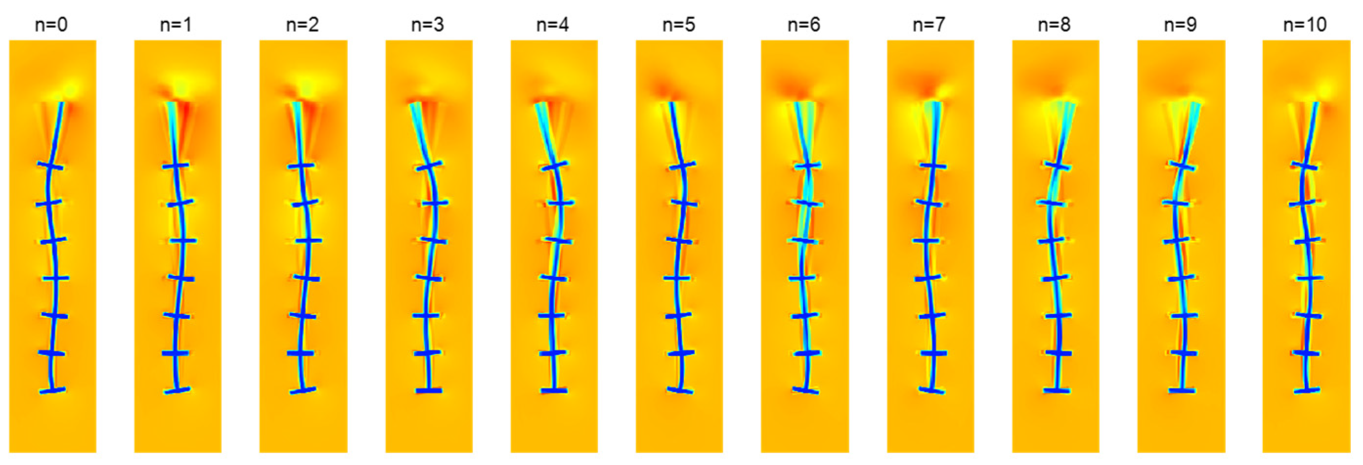
Figure 10.
Illustration of the robot–environment states, , obtained from the SINDy reconstructed data. As before, the time between the snapshots is one-tenth of the period, T.
Figure 10.
Illustration of the robot–environment states, , obtained from the SINDy reconstructed data. As before, the time between the snapshots is one-tenth of the period, T.
Disclaimer/Publisher’s Note: The statements, opinions and data contained in all publications are solely those of the individual author(s) and contributor(s) and not of MDPI and/or the editor(s). MDPI and/or the editor(s) disclaim responsibility for any injury to people or property resulting from any ideas, methods, instructions or products referred to in the content. |
© 2024 by the authors. Licensee MDPI, Basel, Switzerland. This article is an open access article distributed under the terms and conditions of the Creative Commons Attribution (CC BY) license (http://creativecommons.org/licenses/by/4.0/).
Copyright: This open access article is published under a Creative Commons CC BY 4.0 license, which permit the free download, distribution, and reuse, provided that the author and preprint are cited in any reuse.


