Submitted:
15 November 2024
Posted:
18 November 2024
You are already at the latest version
Abstract
Using data of radon accumulation in a chamber with excess volume at one of the points of the Kamchatka subsurface gas monitoring network, the change of radon flux density due to seismic waves and post-seismic relaxation of the medium is shown. Data in the temporal vicinity of a strong earthquake with Mw=7.0, which occurred in the northern part of the Avacha Gulf on 17 August 2024, were used. The study was carried out using methods of mathematical modeling and inverse problem solving. The change in the intensity of radon transport due to changes in the state of the geo-medium is described using the fractional difference operator of constant real order α. As a result of modeling it is shown that strong seismic impact and subsequent processes in the earth crust led to the change of radon flux in the accumulation chamber. The optimal values of the model parameters were determined, which allowed solving the problems of radon flux density determination. An hereditary mathematical model based on fractional derivative has been applied for the first time to estimate the change of radon flux density under the change of stress-strain state of the medium under strong earthquake conditions. The obtained model curves are in good agreement with real data.
Keywords:
mathematical modeling
; radon volumetric activity
; radon flux density
; earthquake precursors
; Gerasimov-Caputo fractional derivative
; memory effect
; nonlocality
; inverse problems
; Levenberg-Marquardt algorithm
; MATLAB
; C
; Gnuplot
MSC: 26A33, 86A22, 49N45
1. Introduction
In today’s world, one of the most dangerous threats to human life is seismic activity, the effects of which can be extremely destructive.
In the Russian segment of the Western Pacific continent-ocean transition zone, two seismogenic structures can be identified that differ significantly in energy and spatial manifestation of seismicity, the Kurilo-Kamchatka and Sakhalin seismic zones. While the former is a subduction zone with possible strong earthquakes with magnitudes up to occurring at depths of 0-700 km, the latter is confined to the western boundary of the Okhotsk lithospheric microplate and is characterized by crustal earthquakes.
For the Kamchatka region the problem of seismicity has the highest priority, as the Kamchatka peninsula is located in one of the most earthquake-prone areas of the Earth. The cities of Petropavlovsk-Kamchatsky, Yelizovo and Vilyuchinsk are located in the zone of 9-point earthquakes, which once again proves the need to develop effective methods of seismic activity forecasting. Strong seismic events can cause a tsunami wave, which can cause great economic damage to the shores of Kamchatka and the Kuril Islands.
A possible way to solve this problem, the development of an effective forecasting system based on an in-depth understanding of the processes occurring in the Earth’s crust in preparation for a future earthquake focal.
One of the methods of studying such processes is monitoring changes in the concentration of radon gas () in the subsurface, atmospheric air and water [1]. Such changes can serve as precursor signals of preparation of strong earthquakes. The study of variations in subsurface air helps to obtain information about geodynamics processes in the mountain massive and properties of the medium through which subsurface gases migrate. Long-term observations and their comparison with the seismicity of the region allow tracking changes in the character of geodynamics processes. This information can be used to search for precursor anomalies that may indicate the approach of a strong earthquake.
One of the uranium decay products is the noble gas . The decay of radon and its products occurs with the emission of three types of radiation, by which its concentration can be measured. Radon is transported into the atmosphere by diffusion and convection.
The Petropavlovsk-Kamchatka geodynamics test site is monitoring on a network of points. The network is created in such a way that the main attention is directed to the Avacha and Kronotsky Bays and the south of Kamchatka. The observation points are equipped with complexes for recording subsurface gases, primarily radon and hydrogen. The network has been operating in different configurations for more than 20 years. On the basis of the obtained data, including volumetric radon activity (RVA) for a number of earthquakes in the Avacha Gulf region, two types of precursor anomalies were identified in the subsurface radon field.
Type A anomalies are characterized by their in-phase manifestation at 3-5 points with a relative shift in time. The most common forms of these anomalies are bay-shaped and stepped, of different polarity. The precursor anomaly of type A was also registered for the deep (origin depth 177 km) Zhupanovskoe earthquake with and for the earthquake on 03 April 2023 with . The possible reason for the appearance of in-phase anomalies on the network of points of registration of subsurface gases are deformation processes such as a solitary ‘deformation wave’, which can arise due to quasi-viscous flow of geomaterial at the last stage of earthquake preparation.
Type B precursor anomalies were registered, as a rule, in one point of the network, had a definite shape and stood out well against the general background. Calculations performed by mathematical modeling methods showed that the mechanism of occurrence of such anomalies is associated with the injection of into the groundwater flow with full transverse mixing under the influence of a deformation stress pulse [2].
Identification of signs of such processes in the data of radon observations is one of the actual tasks of geophysics. Application of new experimental data of subsurface gas variations in comparison with data on seismicity of the region and study of migration processes with the help of the most modern methods of mathematical modeling in order to interpretation of anomalous effects preceding earthquakes is a new and actual method of research in Earth sciences and in particular in development of earthquake forecasting methods.
The earthquake with magnitude has happened on August 17, 2024 at 19:10:26 (UTC) in the northern part of Avacha Gulf, not far from Shipunsky peninsula, later named Shipunsky in connection with geographical location of epicentre (52.931°N, 160.133°E). The epicentral distance to Petropavlovsk-Kamchatsky was 100 km and the depth was 29 km according to the National Earthquake Information Centre (NEIC, U.S. Geological Survey). The intensity of shaking in Petropavlovsk-Kamchatsky was VI-VII points according to seismic intensity scale (SIS).
Before this earthquake, a number of anomalous effects were registered in the subsurface radon field at the network of points [3] near Petropavlovsk-Kamchatsky. The data of radon monitoring before and after this earthquake were used in this work to estimate the changes in the radon flux density in the accumulation chamber.
On (Figure 1) shows the RVA and atmospheric pressure curves. On the RVA curve for estimation of radon flux density, two least noisy areas were selected for exogenous impacts. In the second plot (Figure 1 b), the abrupt release of RVA is associated with the arrival of a cyclone and a decrease in atmospheric pressure. To use these data for modeling purposes, the RVA data were removed at the specified site and the skip was filled in using the Lubushin A.A. software package. [4].
The figure shows that three days before the earthquake there was a sharp decrease in RVA, and then followed by a new stage of accumulation. It is supposed that such behavior of RVA is connected with the last stage of development of the source of future earthquake and is determined by propagation of deformations in the Earth crust. Similar behavior of RVA curves was recorded before a number of strong earthquakes in southern Kamchatka and earlier [3].
The article has the following structure: section 1 presents the introduction, describes the scope and object of the study, and presents the structure of the article; section 2 briefly presents information about radon monitoring as the main method of obtaining experimental data on RVA accumulation used in the study; section 3 describes concepts and models used in mathematical modeling of the RVA accumulation process; section 4 presents the classical mathematical model of RVA, as well as concepts and quantities related to this process, describes the hereditary -model RVA as a generalization of the classical model, formulates the direct problem and the method of its solution; section 5 formulates the inverse problem of restoring the values of several parameters and and describes the method of its solution; section 6 describes the method of estimating the flux density based on the used mathematical models and their parameters; section 7 presents the results of solving inverse problems for and on the basis of different experimental data of RVA, and estimates the flux density on the basis of the recovered values of the hereditary -model RVA; section 8 describes the research contribution and the various sources of funding; section 9 summarizes the study, formulates the conclusions.
2. About Radon Monitoring
It is known that radioactive metal is constantly present in the Earth’s crust. The half-life of this element produces (radon), an inert radioactive gas with a half-life of about 3.85 days. This led to the development of radon monitoring, a special area of emanation and radiation monitoring of geo-medium and processes. Radon monitoring includes measurement of the level of and other radon-forming elements, as well as their distribution in space.
On the Kamchatka Peninsula, a network of observation sites [5] has been deployed to monitor and additional environmental parameters (temperature, pressure, moisture, etc.) that can affect the resulting accumulation curve using accumulation chambers with gas-discharge counters. When planning the locations of subsurface gas monitoring network stations in Kamchatka, special attention is paid to river valleys that run along crustal faults. These zones are characterized by increased permeability, which creates favorable conditions for subsurface gases to escape into the atmosphere, as described in the article [6].
Remark 1.
Analysis of RVA data and related parameters obtained during continuous monitoring is one of the methods of searching for earthquake precursors.
This is due to the fact that RVA is affected by changes in the stress-strain state of the medium through which subsurface gas comes to the surface [7], so is considered a well-known and well-proven indicator of the processes occurring in such a medium [8,9]. Monitoring of as a method of searching for precursors of seismic events has proved itself in recent years [10,11], especially as a short-term precursor (up to 15 days) [12,13].
All points in the network are organized according to a common principle. The sensors are usually located in accumulation chambers (10 liter galvanized bucket) in the aeration zone. When the equilibrium between and its decay products is reached in the accumulation chamber, the intensity of -radiation increases, which increases the sensitivity of measurements. The insignificant convective component of subsurface air in the chamber was ensured by holes in the bottom of the bucket and loose packing of the pipe through which the detector was lowered into the chamber (Figure 2)
Gas-discharge counters are the most common detectors of - and - radiation. The high sensitivity of counters allows to register single quanta of ionizing radiation, and the large output signal is easily registered by recalculation circuits. All this allows passive registration of in subsurface air by -radiation of short-lived products of its decay with a high degree of reliability and rather simple metrology.
Conversion from pulses to RVA is carried out by the empirical formula (Bq/m), where M is the number of pulses registered by -radiation sensors per minute), obtained as a result of synchronous registration by certified radiometers RS-410F by femto-TECH (USA), RRA-01M-03 (Russia) and recorder with GDC-19 detector.
The data used in this work were obtained from the RVA sensor at the INSR point installed in the aeration zone of loose sediments at a depth of 3 m from the day surface [3].
Figure 3.
Experimental RVA data for 14 days, from the INSR observation point obtained before the earthquake during the period: 27 July 2024 (16:00) – 10 August 2024 (15:30).
Figure 3.
Experimental RVA data for 14 days, from the INSR observation point obtained before the earthquake during the period: 27 July 2024 (16:00) – 10 August 2024 (15:30).
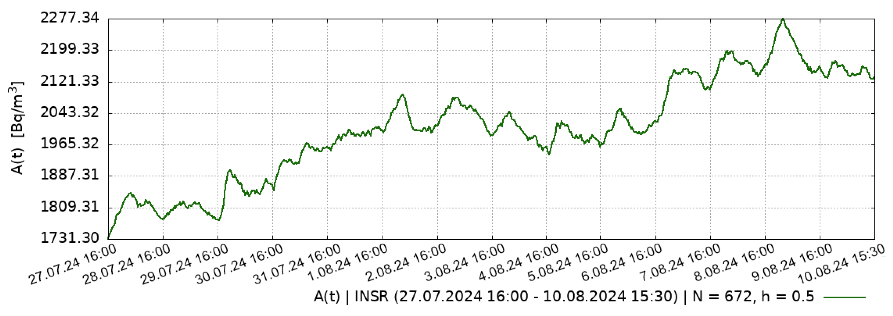
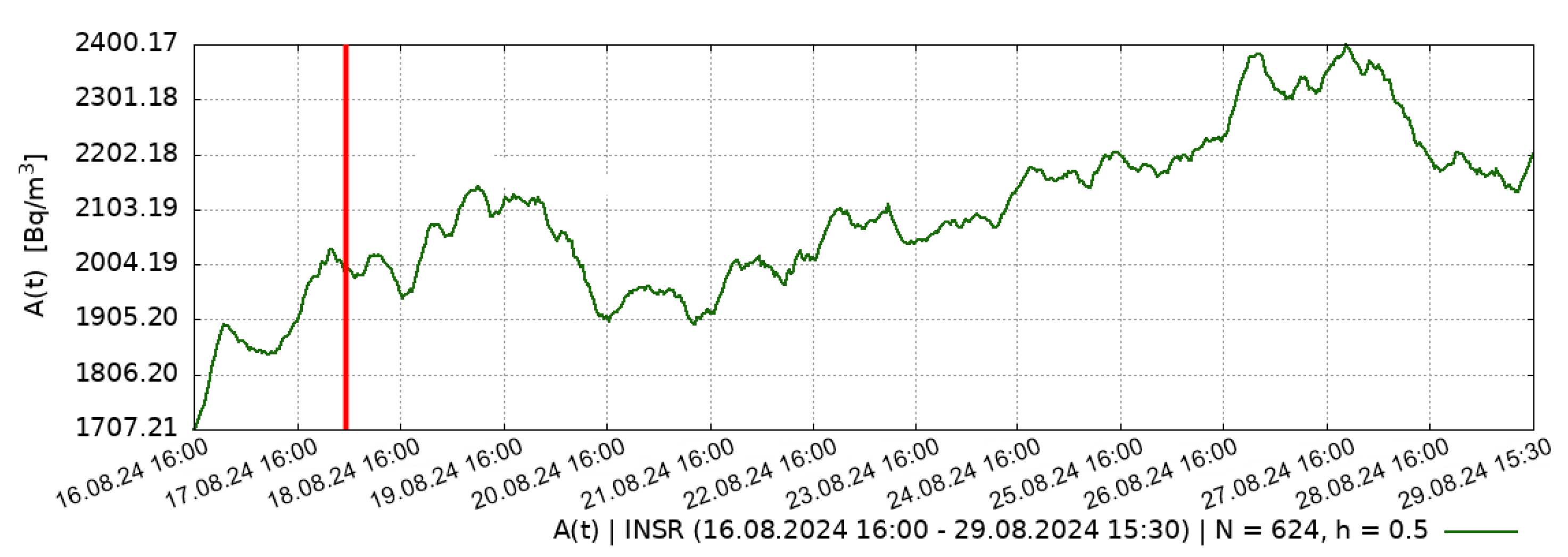
Figure 4.
(green) – experimental RVA data for 13 days, from INSR observation point obtained after the earthquake (include earthquake) during the period: 16 August 2024 (16:00) – 29 August 2024 (15:30); (red) – 7.0 magnitude earthquake.
Figure 4.
(green) – experimental RVA data for 13 days, from INSR observation point obtained after the earthquake (include earthquake) during the period: 16 August 2024 (16:00) – 29 August 2024 (15:30); (red) – 7.0 magnitude earthquake.
3. Approaches used for RVA modeling
The mechanism of transport in geological media is usually considered within the framework of the [14] emanation method and many physical and mathematical models of the [15,16,17,18].
We consider the classical mathematical model of RVA in time in an accumulation chamber based on the equation with ordinary derivative of the 1st order (ODE-model RVA), as well as concepts and quantities related to this process [3,19,20]. This model is the basis for a more generalized process model developed by the authors[2,21]. The weakness of the ODE-model RVA is that it does not take into account changes in the stress-strain state of the medium, assuming that the transfer process occurs in a homogeneous medium.
Remark 2.
In the simplest case, the RVA ODE model assumes a stationary accumulation mode in the chamber, which means that the model must take into account at least – a constant coefficient of air exchange ratio (AER). This is one of the main parameters of both considered RVA models, both ODE and its generalization.
Actually, in order to take into account that the transport of takes place in an heterogeneous medium, the authors earlier [2,21] proposed generalizations of the ODE model RVA using the fractional derivative (FD) apparatus [22,23]. The generalization to the hereditary -model RVA consists in replacing the 1st order ordinary derivative by the Caputo (Gerasimov-Caputo) FD [24,25] of constant order.
The prerequisites for this are several points. First, under the action of tectonic tensions there is a change in the vertical velocity of gas flow[26]. Secondly, the stress-strain state of the medium leads to changes in such characteristics of the geological medium as porosity, permeability, fracturing [2], and the transfer process occurs in such a permeable medium [27].
Remark 3.
Using data when the RVA accumulation curve is clearly visualize and free of noise will allow us to construct model curves that are as close as possible in shape to the real data and with maximum correlation. Therefore, for modeling from (Figure 1) data were selected from time intervals when there were no abrupt changes in atmospheric pressure or winds from cyclones passing by the observation point. Both factors cause blowing of out of the chamber, due to which the RVA curves show <<bumpy>> regions that will interfere with the work of mathematical modeling algorithms, reduce the degree of correlation between model curves and data, and also reduce the accuracy of reconstructed values of and .
The restoration of the parameters and is carried out by methods for solving inverse problems [29,30] from known experimental RVA accumulation data before (Figure 3) and after (Figure 4) earthquake in order to recover the values of the constant parameters and in the hereditary -model RVA, thus testing the hypothesis about the influence of the change in – transport intensity due to the seismic event.
4. RVA models and direct problem statement
In our study, we depend on a well-studied mathematical model of accumulation in an accumulation chamber that effectively describes the accumulation modes [3,19,20]. This model is a linear ordinary differential equation (ODE) of the following form:
where
- – time dependence of RVA in the chamber, [Bq/m];
- – class of continuous-differentiable functions;
- – RVA in outside air, [Bq/m];
- – the current RVA simulation time, [s];
- – total simulation time, [s];
- – some function that describes the rate of entry , i.e., the total specific entry per unit volume of the chamber, [Bq/ms];
- – a function describing the time dependence AER in the chamber, [s];
- – radon decay constant, [s].
As shown in [3,20], the (1) model can be significantly simplified in certain situations. For example, the term at of the equation (1) can be ignored, since even a fully enclosed room with sensors has [h] (i.e., [s]), which is at least an order of magnitude larger than , and thus the effect of the 3rd term of (1) on the calculations of this model is small.
Remark 4.
It is known that the transport of in the vertical direction may be due to thermal-fluid convection, turbulent effects due to changes in meteorological factors, diffusion due to the pressure gradient in the Earth’s crust, diffusion due to the concentration gradient of , and others. [31]. Therefore, in the (1) model, the quantity describes simultaneously the convective and diffusive mechanisms. Since there is no significant convective flow of subsurface air from the surface below the accumulation chamber, the term can be neglected. Which mainly characterizes the accumulation regimes in accumulation chambers.
Remark 5.
The modeled accumulation process can be considered stationary in the sense of the arrival rate when the radon flux density (RFD) from the surface under the accumulation chamber is constant and when there are no dramatic changes in AER. Then the model parameters and are constant values, and the RVA will have an accumulative character with saturation yield: [Bq/m] [3]. From where we obtain that .
Considering the above, the Cauchy problem for (1) takes the form:
where – a known constant, the value of RVA at time .
Remark 6.
Further, when working with experimental data, it will be necessary to make for the time series RVA normalization to the maximum, thus passing for the notation to <<relative units>> [Rel.unit].
Then , and hence the ODE-model will take the form:
Remark 7.
Further, the stationary classical RVA model (2) will be shortly named the ODE-model RVA.
For the Cauchy problem (2), an analytical solution can be obtained:
where at we can see that the RVA .
The (1) and (2) equations use ODE, which significantly limits the flexibility of the ODE model. Therefore, the authors in [2,21] propose a modification of the (2) model consisting in replacing the 1st order ordinary derivative by a fractional derivative of [22,23] of constant order.
Remark 8.
It is assumed that porosity of the medium is due to the presence of isolated pores, and permeability of the medium is understood as the presence of channels conducting gas between the pores. The porosity of the medium can lead to slowing down of the gas transfer process, i.e., subdiffusion, while the permeability of the medium, on the contrary, leads to acceleration, i.e., superdiffusion [14]. Such processes belong to the phenomena of anomalous diffusion [32].
Anomalous diffusion can be related to the property of a system or a medium to remember for some time the impact made on it - [33]. Therefore, the fractional derivative Caputo (Gerasimov-Caputo) [24,25] of constant order is introduced in the mathematical model RVA to describe the heredity:
where is the Euler gamma function:
Remark 9.
A series of works by the authors of [2,21,28] is devoted to investigating issues related to mathematical modeling of RVA, where it is assumed that the parameter describes the fractality of the [36] of the geo-medium and is related to its characteristics such as porosity, permeability and fracturing. The hereditary -model RVA is represented by the following Cauchy problem:
where the difference from (1) is important to note:
- – the solve function, the dependence of RVA on time in the chamber, [Rel.unit];
- – transport intensity , order of fractional derivative (4), dimensionless constant;
- – a class of twice continuously differentiable functions;
- is some positive constant with time dimension [37]. In the following, the work is carried out with undimensionazed and normalized to the maximum, so we assume .
Definition 1.
It is assumed that the order of the fractional derivative α - responsible for the intensity of the transport process , is related to the characteristics of the geosphere: permeability, porosity, fracturing, and possibly also to the fractal dimension, etc. It is assumed that the constant describes the average permeability value of the geosphere under the accumulation chamber of the recording RVA over some volume. Moreover, if , it characterizes less permeable for medium, and if , it characterizes more permeable medium.
Remark 10.
To numerically solve the problem (5), we will use the previously developed nonlocal implicit finite-difference scheme (IFDS) [39] defined in a uniform grid domain:
Definition 2.
Then the difference direct problem:
is a Cauchy problem consisting in finding a discrete function belonging to a known class , with known constants α and .
5. Inverse problem on parameters and for the hereditary -model RVA
Previously, in [2,21,28] the parameters of models and were unknown, and were selected by brute force based on some considerations about the process flow, which is a time-consuming approach. The accuracy of the selection was evaluated by the maximum of – the coefficient of determination [40] and – the Pearson correlation coefficient [41] with the maximum normalized experimental RVA data. This naturally leads to the search for solutions to automate the selection of optimal parameters.
Let (and respectively ) is a function of some known class, but its solution depends on the set of parameters , where , and , . Let the values of the discrete decision function are unknown, but additional information (experimental data of RVA) on the solution of the difference direct Cauchy problem (7) for the hereditary -model RVA is known.
Definition 3.
Then the difference inverse problem for (7) is to recover the values from the known experimental RVA data:
To solve (8), we turn to the unconditional optimization theory [42]. For this purpose, it is necessary to minimize the bias functional:
where is a bias vector of dimension , and the vector is a vector of model data, i.e. the solution of the difference direct problem (7) with respect to some approximation obtained by solving the inverse problem.
The difference inverse problem is solved by a Newton-type unconditional optimization method [43], namely the Levenberg-Marquardt iterative method [44,45], represented as:
where
- – the optimal increment of for the next iteration;
- E is a unit matrix of dimension ;
- – a Jacobi matrix of dimension with elements calculated by the formula: ;
- the derivative is approximated by the difference operator , where – a given small increment of ;
- is the regularization parameter of the method. If and the Hesse matrix H is positive definite, then is the direction of descent for the optimal step of the method;
- Start value: , where v is a given starting constant.
Remark 11.
The solution of the inverse problem (8) by the Levenberg-Marquardt method (10), hereafter (IP-LB), is reduced to starting from the given constants , , v, and c – constants for recalculating γ during the loop, by recomputing the solution of the difference direct problem (7) many times with approximations obtained during the solution of the inverse problem, to compute the optimal values of . More details on the algorithm for implementing the optimization of the vector can be found in the article [46].
The criterion for obtaining the optimal value is , where is the given accuracy of IP-LB solution, – mean square error (MSE) between experimental and model RVA data.
6. About the Flux Density Estimation of
Variations of RVA are related to such indicator as radon flux density (RFD) from the surface under the accumulation chamber. Taking into account Remarks 4, 5 and according to [3] the arrival rate is described by the relation: . Then, to estimate RFD based on a model stationary in the sense of the arrival rate , it suffices to express:
where
- – the arrival rate of into the chamber, [Bq/ms];
- q – RFD from the surface under the accumulation chamber, [Bq/ms];
- – area of flow under the chamber (Figure 2), [m];
- V – volume of the accumulation chamber (Figure 2), [m].
Remark 12.
The parameters of the accumulation chamber at the INSR observation point (Figure 2) take the values: , .
It is also important to note that when working with experimental data RVA is normalized to the maximum [Rel.unit]. But if we want to estimate RFD for the original RVA data, we should substitute the maximum un-normalized value in [Bq/] in place of .
However, the values of AER before the earthquake (Figure 3) and AER after the earthquake (Figure 4) are unknown. But by applying the method described above, it is possible to restore the values of parameters and in the model (5) on the basis of experimental data on RVA variations in the accumulation chamber of the INSR point, and then to estimate the values of before the earthquake and after the earthquake by (11).
Remark 13.
Algorithms realizing solutions of direct problems: by ODE-model (2) and hereditary α-model (5) underlying the IP-LB algorithm, make calculations in <<meter/hour>> values. This is justified by the fact that the actual volume of the storage chamber (∼0.01 [m]) and the frequency of RVA registration (2 cycle./hour). But for convenience of perception, the other parameters of the models (2) and (5) were recorded according to the international system of units SI. Therefore, further in (Figure 5 and Figure 6) parameter values in [h], and the recovered AER value in [h]. Hence, to estimate the RFD (11), we need to divide by 3600 to go to the scale [s].
Then for the camera in (Figure 2) RFD [Bq/s] will be calculated by the formula:
7. Modeling Results
Next, we will present the results of IP-LB solution to restore the optimal values of , of the hereditary -model RVA (5) from known experimental RVA data.
Remark 14.
The restore of is strongly influenced by the choice of its control parameters in the IP-LB algorithm, i.e., – the initial specified approximation and – the initial specified increment of . It was observed that if the initial approximation and its increment are set of the estimate of the maximum value of the parameter to be recovered, the efficiency and accuracy of IP-LB will be the highest based on the estimates of the similarity coefficients for the described data samples.
The results in (Figure 5 and Figure 6) obtained with the following values of control parameters: for the index ; and for the coefficient . The values of the control parameters c, v, described above for the IP-LB algorithm are shown in the figures.
The degree to which the model curves agree well with the experimental data was evaluated by – Pearson correlation coefficient [41] with the processed experimental RVA data used to solve inverse problems. The key parameters characterizing the obtained results are reduced to <<meter/second>> according to the international system of units SI and are summarized in the (Table 1).
8. Contribution to research and funding
Data from the KRMR point were provided by Makarov E.O., senior researcher of the laboratory of acoustic and radon monitoring of the Kamchatka branch of the Federal Research Center <<Unified Geophysical Service of the Russian Academy of Sciences>> Petropavlovsk-Kamchatsky, Russia.
The work was supported by the Ministry of Education and Science of Russia (within the framework of the state task No. 075-00682-24) and with the use of data obtained at the unique scientific installation <<Seismoinfrasound complex for monitoring of the Arctic cryolithozone and the complex of continuous seismic monitoring of the Russian Federation, neighbouring territories and the world>>.
All calculations related to the solution of direct and inverse problems by RVA models, as well as calculations on data processing, were performed in the PRPHMM 1.0 software package in MATLAB [47] version R2023b for GNU/Linux Ubuntu Desktop 22.04. The PRPHMM 1. 0 is developed within the framework of the project <<Modeling of dynamic processes in geospheres taking into account heredity>> at the expense of the grant of the Russian Science Foundation № 22-11-00064 (head Parovik R.I.) implemented at the Institute of Cosmophysical Research and Radio Wave Propagation, Far East Branch of the Russian Academy of Sciences, Paratunka village, Russia.
Visualization in this article was performed by Tverdyi D.A. using the software package FEVO 1.0, developed also in the script language Gnuplot 6.0 [48] for GNU/Linux Ubuntu Desktop 22.04. The software package FEVO 1. 0 is developed within the framework of the project ‘Development of a software package for modeling and analysis of volumetric activity of radon as a precursor of strong earthquakes in Kamchatka’ under the grant of the Russian Science Foundation № 23-71-01050 (head Tverdyi D.A.) implemented at the Institute of Cosmophysical Research and Radio Wave Propagation, Far East Branch of the Russian Academy of Sciences, Paratunka village, Russia.
9. Conclusions
The scientific novelty of the presented article consists in the fact that for the first time an hereditary mathematical model has been applied to estimate the change of radon flux density under the change of stress-strain state of the medium in the conditions of a strong earthquake. Moreover, for the first time estimates of radon flux density were given before and after a strong earthquake.
From the results presented in (Table 1) it can be seen that according to the proposed hereditary -model RVA, the radon flux density increased by , while based on the ODE-model RVA radon flux density estimate shows an increase of .
The performed estimations also showed that the radon flux density increased after the earthquake, which is probably related to the impact of seismic waves on the ground in the area of installation of the accumulation chamber, as well as with the processes of relaxation of the geo-medium, occurring after the seismic event. This impact led to a change in rock permeability in the area of installation of the accumulation chamber and an increase in the total diffusive-convective flow of geogas. Postseismic anomalous changes in RVA associated with the impact of seismic waves were recorded earlier in Kamchatka after the strong Zhupanovskoe earthquake (30 January 2016, ) [3]
Author Contributions
Conceptualization, D.T., E.M. and P.R.; methodology, D.T. and E.M.; software, D.T.; validation, D.T., E.M. and P.R.; formal analysis, E.M. and P.R.; investigation, D.T. and E.M.; resources, D.T. and E.M.; data curation, E.M.; writing—original draft preparation, D.T. and E.M.; writing—review and editing, E.M. and P.R.; visualization, D.T.; supervision, P.R.; project administration, D.T.; funding acquisition, P.R. All authors have read and agreed to the published version of the manuscript.
Funding
This research was funded by Russian Science Foundation grant number 22-11-00064; This research was funded by Russian Science Foundation grant number 23-71-01050; The work was supported by Ministry of Science and Higher Education of the Russian Federation (075-00682-24).
Institutional Review Board Statement
Not applicable.
Informed Consent Statement
Not applicable.
Data Availability Statement
Not applicable.
Conflicts of Interest
The authors declare no conflicts of interest.
Abbreviations
The following abbreviations are used in this manuscript:
| Radon | |
| Radium | |
| NEIC | National Earthquake Information Center |
| UTC | Coordinated Universal Time |
| SIS | Seismic Intensity Scale |
| RVA | Radon Volumetric Activity |
| GDC-19 | Gas Discharge Counter |
| RFD | Radon Flux Density |
| AER | Air Exchange Rate |
| ODE | Ordinary Differential Equation |
| FD | Fractional derivative |
| IFDS | Implicit Finite-Difference Scheme |
| MNM | Modified Newton’s Nethod |
| IP-LB | Inverse Problem by method Levenberg-Marquardt |
| MSE | Mean Squared Error |
References
- Rudakov, V.P. Emanational Monitoring of Geoenvironments and Processes; Science World: Moscow, Russia, 2009; p. 175. (In Russian) [Google Scholar]
- Tverdyi, D.A.; Makarov, E.O.; Parovik, R.I. Hereditary Mathematical Model of the Dynamics of Radon Accumulation in the Accumulation Chamber. Mathematics 2023, 11, 850. [Google Scholar] [CrossRef]
- Firstov, P.P.; Makarov, E.O. Dynamics of Subsoil Radon in Kamchatka and Strong Earthquakes; Vitus Bering Kamchatka State University: Petropavlovsk-Kamchatsky, Russia, 2018; p. 148. (In Russian) [Google Scholar]
- Lyubushin, A.A. Analysing data from geophysical and environmental monitoring systems; Science: Moscow, Russia, 2007; p. 228. (In Russian) [Google Scholar]
- Makarov, E.O.; Firstov, P.P.; Voloshin, V.N. Hardware complex for recording soil gas concentrations and searching for precursor anomalies before strong earthquakes in South Kamchatka. Seismic instruments 2013, 49, 46–52. [Google Scholar] [CrossRef]
- Firstov, P.P.; Rudakov, V.P. Results of registration of subsoil radon in 1997–2000 at the Petropavlovsk-Kamchatsky geodynamic test site. Volcanol. Seismol. 2003, 1, 26–41. (In Russian) [Google Scholar]
- Utkin, V.I.; Yurkov, A.K. Radon as a tracer of tectonic movements. Russ. Geology and Geophys. 2010, 51, 220–227. [Google Scholar] [CrossRef]
- Barberio, M.D.; Gori, F.; Barbieri, M.; Billi, A.; Devoti, R.; Doglioni, C.; Petitta, M.; Riguzzi, F.; Rusi, S. Diurnal and Semidiurnal Cyclicity of Radon (222Rn) in Groundwater, Giardino Spring, Central Apennines, Italy. Water 2018, 10, 1276. [Google Scholar] [CrossRef]
- Neri, M.; Giammanco, S.; Ferrera, E.; Patane, G.; Zanon, V. Spatial distribution of soil radon as a tool to recognize active faulting on an active volcano: The example of Mt. Etna (Italy). J. Environ. Radioact. 2011, 102, 863–870. [Google Scholar] [CrossRef]
- Petraki, E.; Nikolopoulos, D.; Panagiotaras, D.; Cantzos, D.; Yannakopoulos, P.; Nomicos, C.; Stonham, J. Radon-222: A Potential Short-Term Earthquake Precursor. Earth Sci. Clim. Chang. 2015, 6, 282. [Google Scholar] [CrossRef]
- Hauksson, E. Radon content of groundwater as an earthquake precursor: evaluation of worldwide data and physical basis. J. Geophys. Res. Solid Earth 1981, 86, 9397–9410. [Google Scholar] [CrossRef]
- İnan, S.; Akgül, T.; Seyis, C.; Saatçılar, R.; Baykut, S.; Ergintav, S.; Baş, M. Geochemical monitoring in the Marmara region (NW Turkey): A search for precursors of seismic activity. J. Geophys. Res. Solid Earth 2008, 113, 1–15. [Google Scholar] [CrossRef]
- Biryulin, S.V.; Kozlova, I.A.; Yurkov, A.K. Investigation of informative value of volume radon activity in soil during both the stress build up and tectonic earthquakes in the South Kuril region. Bull. KRASEC. Earth Sci. 2019, 4, 73–83. [Google Scholar] [CrossRef]
- Parovik, R.I. Mathematical modeling of the non-classical theory of the emanation method; (In Russian). Vitus Bering Kamchatka State University: Petropavlovsk-Kamchatsky, Russia, 2014; p. 80. [Google Scholar]
- Etiope, G.; Martinelli, G. Migration of carrier and trace gases in the geosphere: An overview. Phys. Earth Planet. Inter. 2002, 129, 185–204. [Google Scholar] [CrossRef]
- Varhegyi, A.; Baranyi, I.; Somogyi, G.A. Model for the vertical subsurface radon transport in «geogas» microbubbles. Geophys. Trans. 1986, 32, 235–253. [Google Scholar]
- Ponamarev, A.S. Fractionation in hydrothermal fluid as a potential opportunity for the formation of earthquake precursors. Geochemistry 1989, 5, 714–724. (In Russian) [Google Scholar]
- Barsukov, V.L.; Varshal, G.M.; Garanin, A.V.; Zamokina, N.S. Significance of hydrogeochemical methods for short-term earthquake prediction. In Hydrogeochemical precursors of earthquakes; Varshal, G.M., Ed.; Science: Moscow, Russia, 1985; pp. 3–16. (In Russian) [Google Scholar]
- Dubinchuk, V.T. Radon as a precursor of earthquakes. In Proceedings of the Isotopic geochemical precursors of earthquakes and volcanic eruption, Vienna, Austria, 9–12 September 1991; IAEA: Vienna, Austria, 1993; p. 9. [Google Scholar]
- Vasilyev, A.V.; Zhukovsky, M.V. Determination of mechanisms and parameters which affect radon entry into a room. J. Environ. Radioact. 2008, 1240, 185–190. [Google Scholar] [CrossRef]
- Tverdyi, D.A.; Parovik, R.I.; Makarov, E.O.; Firstov, P.P. Research of the process of radon accumulation in the accumulating chamber taking into account the nonlinearity of its entrance. E3S Web Conf 2020, 196, 02027. [Google Scholar] [CrossRef]
- Kilbas, A.A.; Srivastava, H.M.; Trujillo, J.J. Theory and Applications of Fractional Differential Equations, 1st ed.; Elsevier: Amsterdam, The Netherlands, 2006; p. 523. [Google Scholar]
- Nakhushev, A.M. Fractional calculus and its application; Fizmatlit: Moscow, Russia, 2003; p. 272. (In Russian) [Google Scholar]
- Gerasimov, A.N. Generalization of linear deformation laws and their application to internal friction problems. USSR Appl. Math. Mech. 1948, 12, 529–539. [Google Scholar]
- Caputo, M. Linear models of dissipation whose Q is almost frequency independent – II. Geophys. J. Int. 1967, 13, 529–539. [Google Scholar] [CrossRef]
- King, C.Y. Gas-geochemical approaches to earthquake prediction. In Proceedings of the Isotopic geochemical precursors of earthquakes and volcanic eruption, Vienna, Austria, 9–12 September 1991; IAEA: Vienna, Austria, 1993; p. 22. [Google Scholar]
- Parovik, R.I.; Shevtsov, B.M. Radon transfer processes in fractional structure medium. Math. Model. Comput. Simul. 2010, 2, 180–185. [Google Scholar] [CrossRef]
- Tverdyi, D.A.; Makarov, E.O.; Parovik, R.I. Research of Stress-Strain State of Geo-Environment by Emanation Methods on the Example of alpha(t)-Model of Radon Transport Bull. KRASEC Phys. Math. Sci. 2023, 44, 86–104. [Google Scholar] [CrossRef]
- Mueller, J.L.; Siltanen, S. Linear and Nonlinear Inverse Problems with Practical Applications; Society for Industrial and Applied Mathematics: Philadelphia, PA, USA, 2012; p. 351. [Google Scholar] [CrossRef]
- Tarantola, A. Inverse problem theory: methods for data fitting and model parameter estimation, Elsevier Science Pub. Co.: Amsterdam and New York, 1987; p. 613.
- Novikov, G.F. Radiometric intelligence; Science: Leningrad, Russia, 1989; p. 406. (In Russian) [Google Scholar]
- Uchaikin, V.V. Fractional Derivatives for Physicists and Engineers. Vol. I. Background and Theory; Springer: Berlin/Heidelberg, Germany, 2013; p. 373. [Google Scholar] [CrossRef]
- Volterra, V. Sur les équations intégro-différentielles et leurs applications. Acta Math. 1912, 35, 295–356. [Google Scholar] [CrossRef]
- Patnaik, S.; Hollkamp, J.P.; Semperlotti, F. Applications of variable-order fractional operators: A review. Proc. R. Soc. A 2020, 476, 20190498. [Google Scholar] [CrossRef] [PubMed]
- Coimbra, C.F.M. Mechanics with variable-order differential operators. Annalen der Physik 2003, 12, 692–703. [Google Scholar] [CrossRef]
- Mandelbrot, B.B. The fractal geometry of nature; W.H. Freeman and Co.: New York, NY, USA, 1982; p. 468. [Google Scholar]
- Rekhviashvili, S.S.; Pskhu, A.V. Fractional oscillator with exponential-power memory function. Lett. to ZTF 2022, 48. [Google Scholar] [CrossRef]
- Tverdyi, D.A.; Parovik, R.I. Application of the Fractional Riccati Equation for Mathematical Modeling of Dynamic Processes with Saturation and Memory Effect. Fractal Fract. 2022, 6, 163. [Google Scholar] [CrossRef]
- Tverdyi, D.A.; Parovik, R.I. Investigation of Finite-Difference Schemes for the Numerical Solution of a Fractional Nonlinear Equation. Fractal Fract. 2022, 6, 23. [Google Scholar] [CrossRef]
- Chicco, D.; Warrens, M.J.; Jurman, G. The coefficient of determination R-squared is more informative than SMAPE, MAE, MAPE, MSE and RMSE in regression analysis evaluation. PeerJ Comput. Sci. 2021, 299, e623. [Google Scholar] [CrossRef]
- Cox, D.R.; Hinkley, D.V. Theoretical Statistics, 1st ed.; Chapman & Hall/CRC: London, UK, 1974; p. 528. [Google Scholar]
- Dennis, J. E.; Robert, Jr.; Schnabel, B. Numerical methods for unconstrained optimization and nonlinear equations; SIAM: Philadelphia, USA, 1996; p. 394. [Google Scholar]
- Gill, P.E.; Murray, W.; Wright, M.H. Practical Optimization; SIAM: Philadelphia, USA, 2019; p. 421. [Google Scholar]
- Levenberg, K. A method for the solution of certain non-linear problems in least squares. Quarterly of applied mathematics 1944, 2, 164–168. [Google Scholar] [CrossRef]
- Marquardt, D.W. An algorithm for least-squares estimation of nonlinear parameters. Journal of the society for Industrial and Applied Mathematics 1963, 11, 431–441. [Google Scholar] [CrossRef]
- Tverdyi, D.A.; Parovik, R.I. The optimization problem for determining the functional dependence of the variable order of the fractional derivative of the Gerasimov-Caputo type Bulletin KRASEC. Physical and Mathematical Sciences 2024, 47, 35–57. [Google Scholar] [CrossRef]
- Ford, W. Numerical linear algebra with applications: Using MATLAB, 1st ed; Academic Press: London, UK, 2014; p. 628. [Google Scholar] [CrossRef]
- Janert, P.K. Gnuplot in Action: Understanding Data with Graphs, 2nd ed.; Manning: New-York, 2016; p. 400. [Google Scholar]
Figure 1.
(green) – Experimental OAR data from the INSR observation site, in the temporal vicinity of the 50-day earthquake: (a) – RVA before earthquake, during 27 July 2024 (16:00) – 10 August 2024 (15:30); (b) – RVA after earthquake, during 16 August 2024 (16:00) – 29 August 2024 (15:30); (grey) – atmospheric pressure data at INSR point; (light blue) – excised section of the OAR due to the strong influence of reduced pressure; (red) – 7.0 magnitude earthquake.
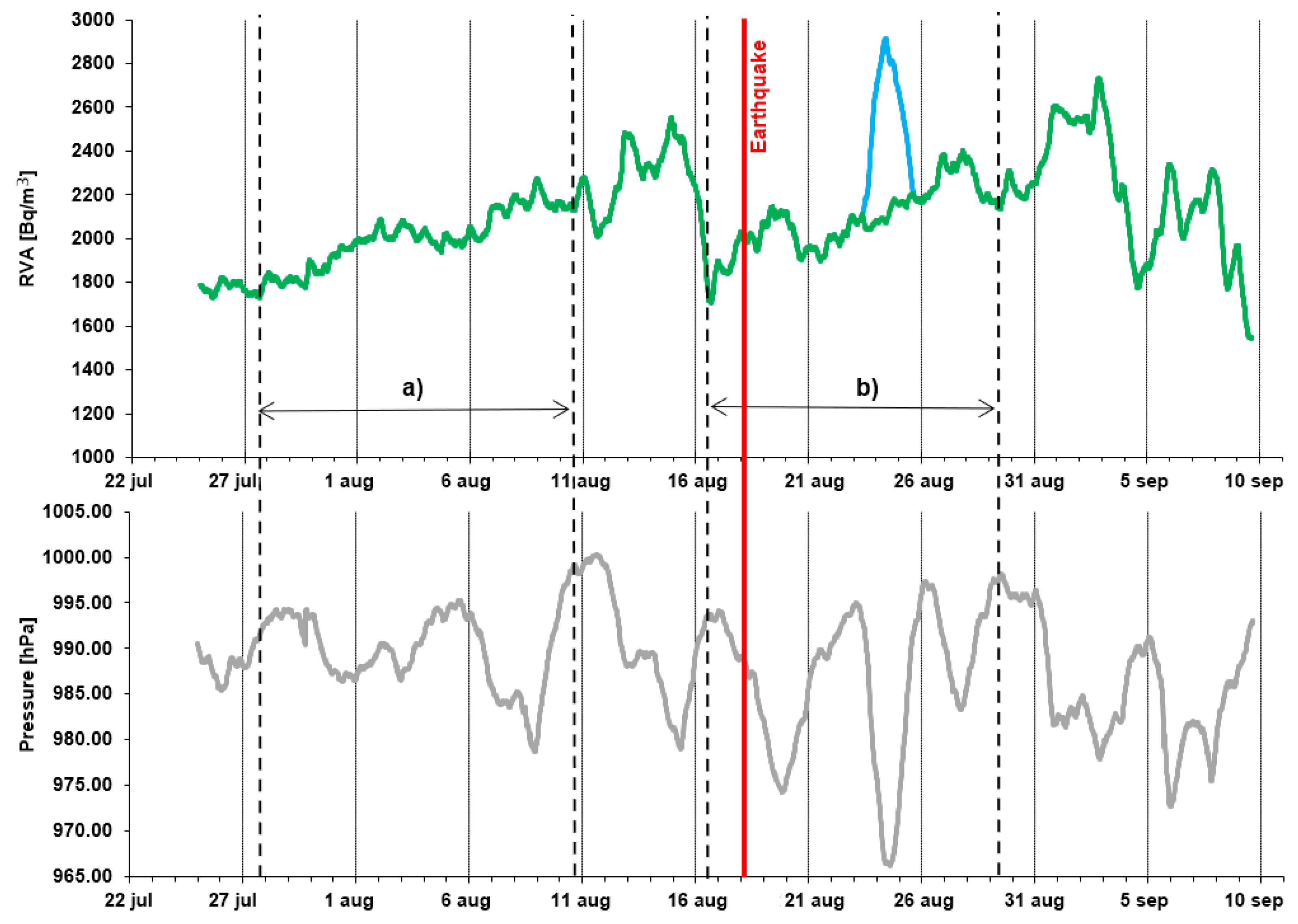
Figure 2.
Scheme of placement of GDC-19 gas-discharge detectors for registration of -radiation of radon decay products.
Figure 2.
Scheme of placement of GDC-19 gas-discharge detectors for registration of -radiation of radon decay products.
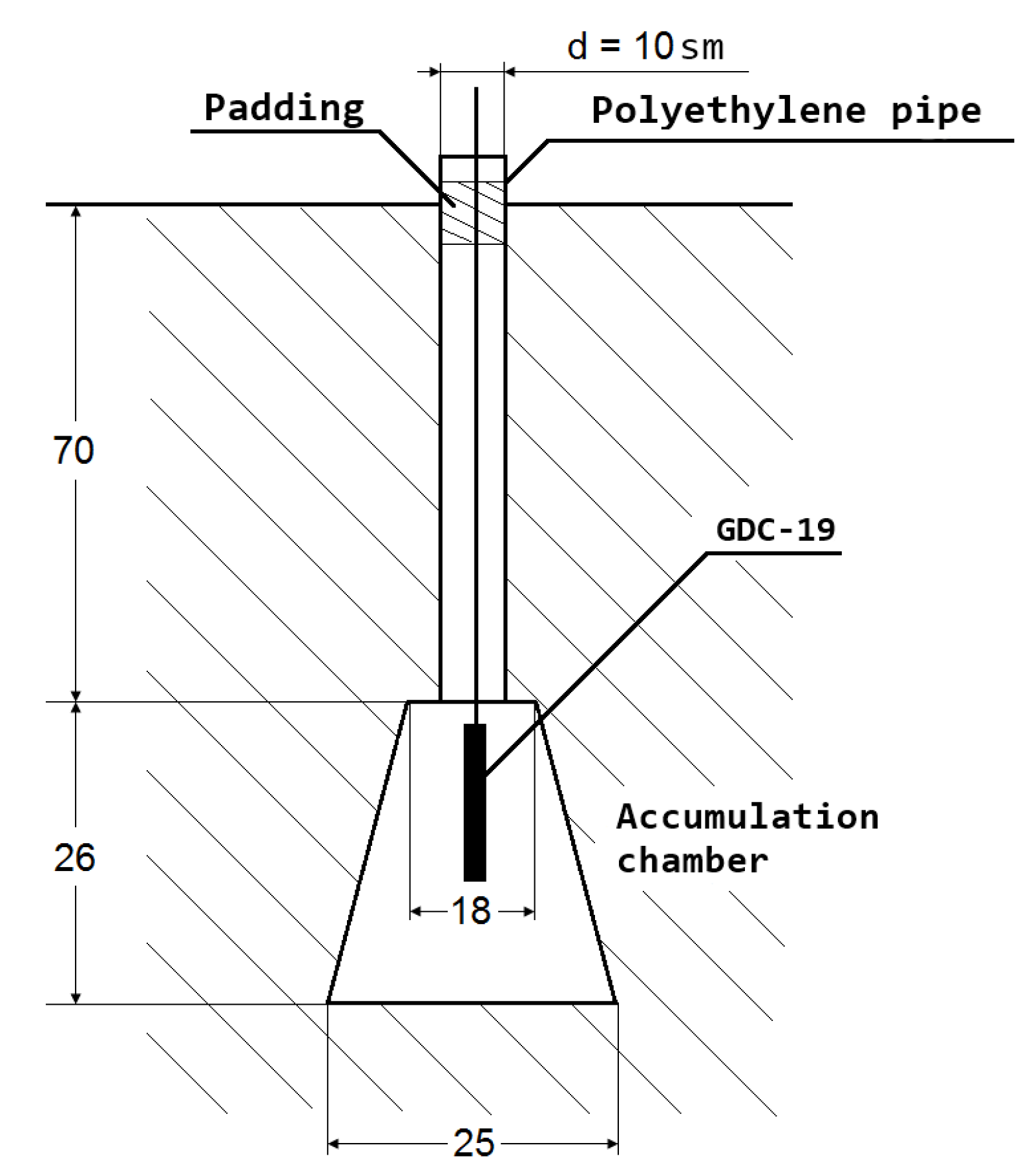
Figure 5.
Modeling results based on RVA data before the earthquake.
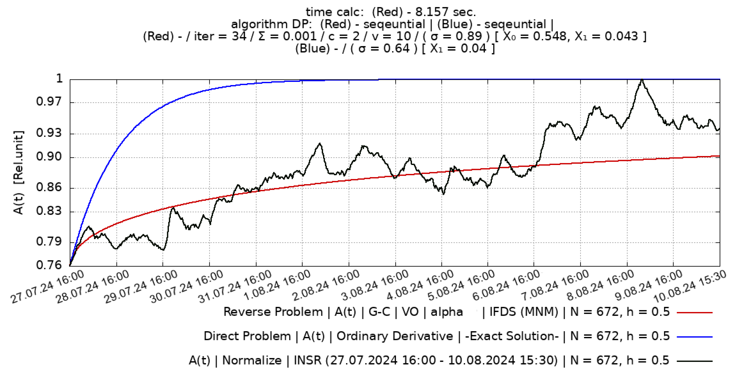
Figure 6.
Modeling results based on RVA data after the earthquake.
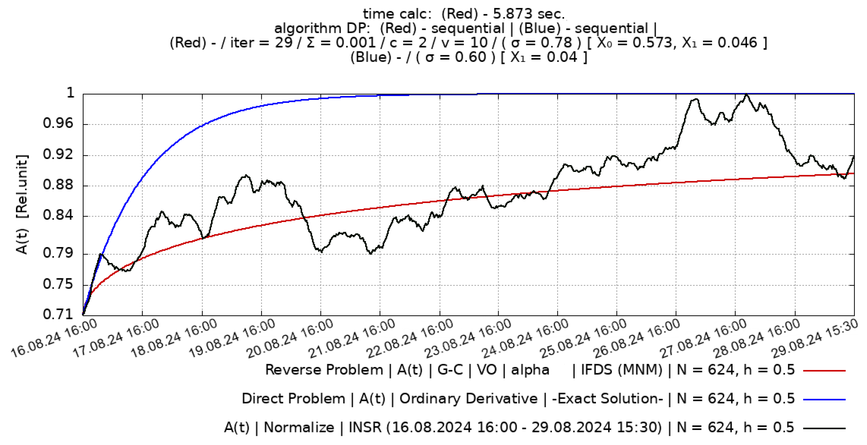

Table 1.
Parameters of mathematical models: classical ODE (2), hereditary -model RVA (5) solved by methods of inverse problems, as well as similarity coefficients of model curves and data.
| INSR dates data sampling |
|
Set for ODE |
Restore for heredity |
for ODE |
for heredity |
for ODE |
for heredity |
RFD by ODE |
RFD by heredity |
|---|---|---|---|---|---|---|---|---|---|
| Before: 27.07.24 - - 10.08.24 |
2277.34 | 1 | 0.548 | 64 % | 89 % | ||||
| After: 16.08.24 - - 29.08.24 |
2400.17 | 1 | 0.573 | 60 % | 78 % |
Disclaimer/Publisher’s Note: The statements, opinions and data contained in all publications are solely those of the individual author(s) and contributor(s) and not of MDPI and/or the editor(s). MDPI and/or the editor(s) disclaim responsibility for any injury to people or property resulting from any ideas, methods, instructions or products referred to in the content. |
© 2024 by the authors. Licensee MDPI, Basel, Switzerland. This article is an open access article distributed under the terms and conditions of the Creative Commons Attribution (CC BY) license (http://creativecommons.org/licenses/by/4.0/).
Copyright: This open access article is published under a Creative Commons CC BY 4.0 license, which permit the free download, distribution, and reuse, provided that the author and preprint are cited in any reuse.


