A Hybrid Approach to Dark Matter based upon Hawking’s Cosmology, a Natural Explanation and Improved Prediction Algorithm for Galaxy Flat Rotation Curves and Cluster Velocity Dispersions

1. Introduction

The hypothesis of dark matter is a way to explain why among other galaxies seem not to obey Newton’s law of gravity. As well, dark matter is needed to explain the statistical distribution of ‘cold’ and ‘hot’ spots in the background radiation, that would still need the existence of (much) dark matter vs. baryonic matter to be understandable in terms of Big Bang nucleosynthesis, as well as matters like gravitational lensing.

Nevertheless, there exist several alternative approaches to account for the additional gravity it yields, like Modified Newtonian Dynamics (MOND) [1,2], Bekenstein’s TensorVectorScalar gravity (TeVeS) [3] or Covariant Emergent Gravity (CEG) [4]. But, they assume dark matter does not really exist, and so leave the other matters mentioned up here, and the gravity in galaxy clusters, see Banik [2], unresolved. Besides that, they do not give a natural explanation for the concepts and additional fields they introduce.

Therefore, in the article in hand the existence of dark matter is the starting point.

As recommended by Banik in Symmetry [2], a hybrid approach will be presented. It is based upon the real existence of dark matter and so as to describe its effect on gravity, it applies the cylindrically symmetric solution of the Einstein field equations from Levi-Civita [5] as described by Santos [6]. It will be argued that it logically follows from Hawking’s Cosmology [7,8]. It solves the problem that Lelli and Mistele [9] showed, that the common way to project dark matter halos around galaxies cannot be valid, since the alternative naturally assumes dark matter is distributed like the visible matter in a galaxy, but in a wire-mass shape, consistent with [5] and [6]. The hypothesis gives a natural explanation of dark matter, why it is undetectable and why its gravity shows behaviour as described in general by TeVeS theory, which in the Newtonian limit resembles MOND and is employed as well in the paper in hand. The term naturalness is extensively discussed by Hossenfelder [10] (p. 57). In short it means that a theory is without fine-tuned constants.

General Relativity (GR) in galaxies seems to need the said halos too so as to properly include the effect of dark matter, but in this paper an alternative is proposed and argued: three orthogonal wire-masses of dark matter through the galaxy centre based upon [5] and [6]. Or, alternatively, GR must be modified with some additional terms to make correct solutions possible without these halos. Bekenstein’s TeVeS [3] follows that path and is employed in this paper too because he studied the evolution in time, but only as a mathematical description of dark matter. This goes together well with this hypothesis, since it considers dark matter to be in the galaxies in the form of a wire-mass, described by a linear mass density, attracted by the visible matter, instead of in halos. This is why this hypothesis is called hybrid in the above.

In this paper the Spitzer Space Telescope satellite data of 175 galaxies, SPARC, as processed and reported by Lelli et al. [11] and Starkman et al [12] are used to assess several predictions that follow from this theory. The mass-to-light ratio has been used as the only fitting parameter to fit the baryonic rotation velocity, and hence the baryonic gravitational acceleration, in each galaxy to the observed values near the centre of the galaxies. After that, the hypothesis in hand is used to predict the additional gravitational acceleration at all radii without any further fitting and to compare the predictions with the observed values.

After a brief introduction of Big Bang theory in chapter 2.1 and Hawking’s cosmology in chapter 2.2 and some other indispensable literature about quantum systems in chapter 2.3, MOND and TeVeS will be discussed in chapter 2.4. This forms the fundament for the proposal presented in chapter 3.

In chapter 3 the proposal will stepwise be derived in a logical manner from Hawking’s cosmology and String theory. In chapter 4 this will all be worked out. Firstly, an interpretation of the MOND like behaviour of dark matter as a sum of two fields will be proposed. Secondly, the natural basis for this will be explored in chapter 4.2 and in chapter 4.3. In the rest of chapter 4, the hypothesis for dark matter will be elaborated and its consequences and behaviour will be explored.

In chapter 5, six testable predictions are proposed and proved, one using the work of Levi-Civita, and in chapter 5.3 an improved alternative to MOND for the prediction of rotation velocities in the Newtonian limit as well as velocity dispersions in clusters is presented.

In chapter 5.4 TeVeS will be elaborated and used to prove a prediction about the evolution in time of the gravitational acceleration by dark matter. It will be shown this prediction gives a much improved prediction for dispersion velocities in a wide range of NGC and Abell clusters.

In chapter 6 the conclusions and suggestions for further work are presented.

2. Hawking´s Cosmology and Superposition State of Universe, MOND and TeVeS

In this chapter the fundament for the proposal of chapter 3 will be laid, by giving an overview of existing theories that contain vital building elements.

2.1. Big Bang Theory

The line of thought of the universe as a quantum system is an elaboration of Hartle & Hawking [7]. The universe, according to the Big Bang theory, comes from an infinitesimal small point in which only elementary particles existed in the form of a plasma, with an extremely high temperature [13] (pp. 127-136) and as a result was in a quantum state, see chapter 4.

The originally extremely high temperature is still visible and measurable in the so-called background radiation. Its properties are direct evidence that the universe originated from a hot Big Bang stage. The Big Bang theory is also a logical extrapolation of the expansion of the universe that we observe, among other things due to the redshift of the spectrum of the radiation of stars, but also of the history/evolution of stars and galaxies as visible through our telescopes. In addition, the non-uniform distribution of stellar objects as quasars over the different redshifts proves the universe is not static.

Moreover, Big Bang theory can quantitatively explain many phenomena, such as the distribution over the various elements of the mass in the universe, the cosmic composition, based on nuclear physics. The fact that it is dark at night also proves that the universe cannot be infinitely large and infinitely old, because then the entire sky would be filled with light from stars. So, our universe indeed has a beginning. Moreover, the Big Bang theory forms a well-cohesive whole with astronomy and the rest of physics.

2.2. Hawking´s Cosmology and String Theory

Somewhere at the beginning, our universe has been in a quantum state, because that's where one ends upon extrapolating the expansion of the universe back to the very smallest starting point, [7,8] have derived solutions to the wave function of the universe as proposed by Everett [14] and further elaborated by DeWitt [15]. As derived and explained by Hartle & Hawking [7] these solutions must satisfy the Wheeler-DeWitt equation.

Hartle & Hawking [7] show the Wheeler-DeWitt equation has the following form:

$\mathrm{Ĥ}\mathrm{ }\left(x\right)\mathrm{ }|\mathrm{ѱ}\mathrm{ }⟩=0$                                              (1)

Where $|\mathrm{ѱ}⟩$ is the wave function of the universe and where Ĥ(x) is called the Hamiltonian constraint, [7]. The Hamiltonian, in this case derived from General Relativity [7], describes the total energy of a system and $Ĥ$ is the Hamiltonian operator [16] (p. 27). The so-called constraint described by (1) follows from the total energy of the universe being zero, gravitational energy cancelling out the mass energy. Hawking’s & Hartle’s solutions of this equation describe a universe that has no beginning, the Hartle-Hawking state, [7]. Hawking [8] explains this in simpler terms as well: time must have been indeterminate there on the smallest scale in that quantum state, because of the extreme gravitational warpage of space-time at that moment, [8] (p. 172). The time t=0 therefore is not precisely defined and at these scales time reduces to a fourth spatial dimension.

So, the universe has no exact measurable beginning. Hawking calls this the ‘no-boundary-condition’, [8] (pp. 172-173). It makes it impossible to trace the development of our universe from the beginning to this time in a deterministic ‘bottom-top’ way and, hence, there is a need for a statistical ‘top-down cosmology’, considering all possible alternative histories of the universe.

He states that as a consequence of this, at the very beginning time acted as a fourth spatial dimension, ”In the early universe-when the universe was small enough to be governed by both general relativity and quantum theory, there were effectively four dimensions of space and none of time”, [8] (p. 172) This is the starting point of the proposal of this paper. String theory, however, suggests as much as eleven dimensions, but using the minimum of four is more economical and easier to understand.

The quantum aspects of the Big Bang become clearer when considering so-called ‘double-slit’ experiments, with a light beam split in two that are directed at a wall with two narrow slits. Especially the variant where only one photon is fired at a time. The same interference patterns then arise as with continuous beams of photons, so the probability waves of single photons interfere with themselves, as it were. One photon behaves as if it passed through both slits. That can only happen if the photon itself follows all possible alternative paths simultaneously, as it were like a split probability wave. So, the behaviour of the single photon can be seen as a superposition of all possible alternative paths it follows, so alternative histories, [8] (p.104). The superposition causes wave interference and that determines the paths the photon follows in the experiment.

Hawking’s and other’s point about the probabilities is that a quantum experiment will only have a certain outcome when it is performed. The Big Bang can be regarded as such an experiment [8] p. 179), where the universe in the quantum state may have had a statistical probability distribution of many ‘alternative histories’, following the interpretation of Feynman. Maybe 10⁵⁰⁰ ones as String theory and the more general M theory suggest, [8] (pp. 152 and 181). At page 77 Hawking states that “the universe does not have a single existence or history, but rather every possible version of the universe exists simultaneously in what is called a quantum superposition”.

This does not a-priori imply we still are in a real a state of superposition between all, or part of these alternative histories now, but this paper will argue that this is indeed the case with our universe for a specific part of these histories.

The parameters and hence the quantum state of our universe are known now. Our universe has known single values for the fundamental parameters and constants. Of all the ‘alternative histories’, ours is the one that has come true. The experiment has been performed; we know the outcome. This is only possible when there is an observer to the experiment, [8] (pp. 107 and 179). This where the idea of an ‘observed universe’ of Hawking and others like Wheeler comes from. The assumption is that man or other sentient beings can perform this role of external observer, as Hawking and Wheeler argue, based upon the ‘delayed-choice’ experiment by Wheeler, see Zeilinger’s overview [17]. That shows that the moment of time where the observer enters the history is not relevant [8] p. 106-107), which is consistent with Zeilinger’s interpretation and conclusions in [17] and the citation in chapter 5.5.

The ideas in Hawking’s cosmology [7] are consistent with certain approaches to quantum gravity, such as String theory. The idea from Hawking that space and time are quantum phenomena are central themes in quantum gravity research. The Feynman path integrals that Hawking uses, are an important computational method in quantum gravity, especially in the context of Euclidean quantum gravity. This is explained by himself in [7]. This work provides an early foundation for later developments in quantum cosmology, like String theory, and the idea that gravity itself is a quantum phenomenon. From String theory, the assumption in the article in hand of more dimensions in a multiverse has been taken over, which thus is consistent with taking Hawking’s cosmology as a starting point for the theory of the article in hand. But, there yet is no direct evidence for String theory. Future experiments in gravitational waves, particle physics and cosmology could provide clues. If the LHC or future accelerators find supersymmetry, it would be a boost for String theory and hence the assumption of the article in hand.

But, String theory does shed light on the behaviour of black holes. Strominger and Vafa [18] in 1996 showed that in String theory the entropy of certain extremal black holes exactly matches the Bekenstein-Hawking formula [18]. They calculated the number of microscopic states of D-branes and found a perfect match.

Maldacena [19] in 1999 introduced the AdS/CFT correspondence, a duality rooted in String theory, that couples gravity in a (D+1)-dimensional anti-de Sitter space to a D-dimensional conformal field theory. This idea has major implications for the so-called black hole information paradox. The black hole information paradox is the problem that, according to Hawking's calculations, information appears to be lost when a black hole evaporates due to Hawking radiation, which violates the laws of quantum mechanics that require that information is always conserved. Maldacena’s duality suggests that information is not lost but remains encoded in the dual theory.

Mathur [20] in 2003 proposed that black holes do not contain a singularity, but instead consist of a complex collection of string states, or a fuzzball. This potentially solves the information paradox, because information can be stored in the quantum structure of the fuzzball instead of being destroyed in a singularity. This all is support for the String theory and hence for the assumptions it makes.

In the meanwhile, it is fruitful to explore the potential for a natural explanation of what dark matter is, as is done in the article in hand.

2.3. How a Superposition State Can Have Classical Effects

Quantum superposition can be forced by a beam-splitter like in the famous ‘double-slit’ experiment discussed up here. It can be forced as well by a dedicated device like in a Qubit or in an MRI-scanner. A tensor-interaction like in the deuteron may as well yield a superposition state. The latter will be discussed into more depth in the sequel, since it might be very relevant to the behaviour of our universe. So, quantum effects can affect classical effects through a variety of mechanisms, with microscopic quantum phenomena affecting macroscopic classical phenomena.

A deuteron Is a bare proton and a neutron, glued together, without electrons. It forms a vital step in the fusion of helium, and thus of the existence of stars. The binding force between the neutron and the proton is the sum of the resulting forces of the superposition of two quantum spin states, see Bethe [21]. So, this force would not be strong enough if the deuteron were in just one of those states. It is evident this has a huge classical impact.

Another example is superconductivity. Superconductivity occurs when electrons behave as a collective quantum mechanical entity, completely eliminating electrical resistance. This has applications in powerful magnets and lossless current transport, Ginzburg et al [22].

In the early stages of the universe, quantum fluctuations caused variations in the density of matter, which later evolved into the large-scale structures of the universe such as galaxies and clusters, Guth [23].

Chemical reactions, enzymatic processes and even biological phenomena such as photosynthesis are influenced by quantum mechanical principles, which has macroscopic consequences, McFadden et al [24].

This all is essential to the following part of this paper: as with the single photon in the double-slit or with the deuteron, our universe could still be in a superposition of multiple histories. The result should be able to interfere with itself very well like the single photon, and forces like gravity might add up like in the deuteron. It will be argued why for electro-magnetism this cannot have a measurable impact.

These possibilities for classical effects lead to a testable hypothesis of the nature of dark matter. But firstly, MOND and TeVeS theories are briefly visited, because they give a mathematical description of the gravitational effects of dark matter of which some starting points are used in the article in hand.

2.4. Introduction to MOND and TeVeS Theories

Modified Newtonian Dynamics (MOND) is an empirical alternative to the hypothesis of dark matter to explain why galaxies and open clusters seem not to obey Newton’s law of gravity, see Kroupa [25]. It is explored in this chapter and among other described by Schilling [26].

First published in 1983 by Milgrom [1] and extensively assessed by Banik [2], the aim was to explain why the observed velocities of stars in galaxies are larger than expected based on Newtonian gravity.

An example of the so-called ‘rotation curves’ discussed down here, is shown below in Figure 1. It shows the rotation velocities as a function of radius from the centre of a galaxy, as well as the logarithmic brightness curve, which is a good measure for radial mass distribution. It comes from Lelli [11]. It is one of the 175 galaxies of the SPARC database (NGC6503). The black dots are observed velocities, to be called V_obs in the sequel. They are higher than the velocities calculated from gravitational attracting force according to Newton’s law of gravity. Taking this equal to the centrifugal force, results in the theoretically expected velocity, called V_bar, the blue line.

If at large radii both the total observed gravity decrease linearly with radius, just like the opposing centrifugal force, the observed velocities, V_obs, can remain constant over a long range of radii as can be seen in Figure 1 and Figure 10 and as is shown by Lelli et al [11,12] for many of the other galaxies with Spitzer photometry. See Annex 3 for all the rotation curves.

Milgrom noted that instead of assuming dark matter to solve this, the discrepancy might be resolved if the gravitational force experienced by a star in the outer regions of a galaxy would vary inversely linearly with radius R (as opposed to the inverse square of the radius, as in Newton’s law of gravity). MOND has been fitted empirically such that it differs from Newton’s laws at extremely small accelerations that are characteristic of the outer regions of galaxies with formula (2). The transition would occur below an acceleration of a_m = 1.2 x 10^-10 m²/s, Milgrom’s constant. The area with lower gravitational acceleration is called the MOND regime. The theory needs an interpolation algorithm for the acceleration beneath a_m. The interpolation depends on the variable µ ($x$) with  $x={\displaystyle \frac{g}{a_m}}$ , so the predicted total acceleration over Milgrom’s constant, as follows:

$\mathrm{\mu }\left(x\right)={\displaystyle \frac{x}{\sqrt{1+\mathrm{ }{x}^2}}}$                                                      

(2) and the Newtonian acceleration g_N is related to the resulting total predicted acceleration a through:

$g_N=\mathrm{ }\mathrm{\mu }\mathrm{ }\left(x\right)g\mathrm{ }$                                                           (3)

Since this equation needs to be solved iteratively when it is used to predict the total acceleration from the Newtonian, and since this interpolation formula allows for inversion, it can be rewritten as follows:

$g=g_N\mathrm{ }{\left({\displaystyle \frac{1}{2}}+\mathrm{ }{\displaystyle \frac{1}{2}}\sqrt{1+{\left(2\mathrm{ }{\displaystyle \frac{a_m}{g_N}}\right)}^2}\right)}^{{\displaystyle \frac{1}{2}}}$                                                       (4)

See for example Platschorre [27]. With back and forth calculating a series of values for $a_0$and $a$it can easily be shown that this formula works correctly.

In terms of the Newtonian gravitational potential of the visible matter, $\nabla {\Phi }_N$, this can be written as follows [3]:

$\mu \left({\displaystyle \frac{\left|g\right|}{a_m}}\right)g=\mathrm{ }-\nabla {\Phi }_N$                                                                 (5)

Bekenstein [3] uses a parameter y = |$\nabla \Phi$|²/a_m² which equals x². So: µ($\sqrt{y}$) or simpler µ(y), which will be used in the sequel. He gives an alternative for µ(y) resulting from formula (2).

However, this MOND theory of gravity does improve the calculations on the velocities of stars but does not explain the observed deviations from Newtonian mechanics. Bekenstein even states it is not a theory at all, but only a recipe [3]. Furthermore, as Bekenstein [3] mentions it does not specify how to calculate gravitational lensing by galaxies and clusters of galaxies, and it violates conservation of momentum. For the latter, a theory derived from an action principle is needed.

Early attempts to generalise MOND by making a relativistic version of it were relativistic AQUAL [3] (p. 22) and Phase Coupled Gravity (PCG) [3] (p. 22). Fascinating is that PCG yields a description of total gravity as a sum of two competing fields, one with quadratic decay of gravity with distance x and one that decays linearly [3] (formula (17) at p. 7). This is consistent with formula (7) in the next chapter.

It is interesting to note that Covariant Emergent Gravity (CEG) [4] as well yields a sum of two competing fields, as Platschorre [27] shows. Zhou et al [28] found this as well upon applying a conformal gravity approach.

But both AQUAL and PCG attempts had problems like waves propagating faster than light and incorrect light deflection [3]. Bekenstein provided a theory, that accounts for this, TeVeS, which has been formulated in terms of GR with additional scalar and vector fields [3] and which in the Newtonian limit gives the same results as MOND. This mathematical framework will be successfully applied to the linear gravity hypothesis to study the evolution in time in chapter 6.3 in the scope of the hybrid approach.

However, TeVeS still does not give an explanation for the source of the additional scalar and vector fields. The paper in hand, presents a hypothesis that provides a natural explanation, one that does not need any interpolation algorithm and that significantly can improve the MOND predictions for all galaxies in the SPARC database. It is presented in chapter 3 and worked out in chapter 4.

3. A Hypothesis on the Nature of Dark Matter

The thoughts leading to the hypothesis can be logically summarized as follows, and will be elaborated in the next chapter:

• Hawking’s cosmology is a logical combination of two well proven theories, quantum mechanics and Big Bang theory, and thus, it is a good description of the earliest stages of our universe.
• Our universe results from a Big Bang that was in a quantum superposition state at its start, that can be interpreted as 10⁵⁰⁰ alternative histories in an 11-dimensional space, using the Feynman interpretation of quantum mechanics and String-theory.
• The realization of our universe from the 10⁵⁰⁰ alternative histories cannot have occurred without a sentient observer.
• Our universe has been realized.
• At least one sentient observer exists, which can have come into being in the universe following the conclusion of Wheeler’s delayed choice experiments.
• Since it is not economical to consider 10⁵⁰⁰ a fine-tuned number, aimed at creating exactly one universe with sentient being, there still remains a superposition state of more than one alternative histories of the universe. This makes it a multiverse, each universe with sentient beings. This multiverse still exists by means of a state of superposition, which must not necessarily be disturbed by de-coherence, since nothing exists outside the multiverse.
• The other universes in superposition can follow a history comparable with ours that leads to sentient beings, but do not necessarily share all our spatial dimensions in the 11-dimensional space, but do have nearly exactly the same constants of nature. From the delayed choice experiment it follows they all have the same causal status.
• The gravity of these superposed 11-dimensional universes acts together just like the binding force in a deuteron and as a result the gravitational accelerations and potentials caused by baryonic matter in these universes should be added.
• Since there are more ways to yield partly overlapping universes in an 11-dimensional space than fully overlapping, the odds are that there exist multiple universes that share only one or two dimensions with our universe.
• Gravity acting in our universe resulting from the mass in a 2-dimensional cross section of another one, must act through such a 2-dimensional cross section and hence leads to a linear decrease of the gravitational acceleration as a function of distance from such a mass and hence to a logarithmic potential.
• The existence of multiple universes that share two dimensions with our universe in a state of superposition, forms a natural explanation of what dark matter is and together with the previous step to and explanation for the flat rotation curves at large distances from the core of galaxies.

An argument like this is as strong as its premises. Therefore, the word proof or evidence is avoided here and it is called an argument. In the sequel, this path of thinking will be further worked out and the premises explained.

4. An Elaborated Proposal for Dark Matter

Firstly, in chapter 4.1, the underlying natural explanation for this concept will be presented after the basic assumptions from Hawking’s cosmology and the String theory that was developed from it, will be explored and then the consequences for the gravitational potential will be worked out with help of some concepts from MOND.

4.1. Exploring the Logical Consequences of Hawkings’s Cosmology and String Theory

In the sequel, the case is argued for a natural explanation for the MOND-like behaviour explained in the previous section, starting from this cosmology, String theory that is founded in it and the other elaborations made about superposition in chapter 2. This will not only merge to a natural explanation but yield an improvement of MOND too, in the form of a simple physical model.

The crucial observation of the paper in hand is that if the moment of time where the observer enters the history is not relevant, as discussed in chapter 2.2, this would give all possible observers the same causal status.

Now, it is of paramount importance to realize that there is no natural relationship between the numbers 1, for one universe, and 10⁵⁰⁰ for the number of possibilities, mentioned in chapter 2. Arguing that this number can only lead to one single universe with sentient beings, has created a fine-tuned number, which is not the most economical of explanations, since it would require more explanations itself.

If a universe in which man originated is a realization of 10⁵⁰⁰ possibilities, it is irrational to assume that not at least one more history of the universe, with sentient beings who can also act as observers, has been realized. Who was first or last does not play a role in this, as the 'delayed choice' experiments show. We are then in a multiverse, which state of real superposition, as defined by [8] (p. 77), would result necessarily from the existence of multiple observers. The superposition has then been maintained in the way presented earlier in this essay. The real superposition must necessarily exist if man is the needed observer of our universe. The states will be able to interact with our universe by adding up certain effects, as in the deuteron or the double-slit experiments.

The additional gravity attributed to dark matter can be such an effect. The constants of nature in those universes will have nearly exactly the same value as ours, since the existence of sentient beings does not allow very different values, as explained by [8] (chapter 7 p. 203 in particular) and by Rees in Just Six Numbers [29].

When one would argue that universes can never get in a superposition state, one ends in a ‘reductio ad absurdum’. There must necessary be a real superposition, but there cannot be one…

But, the values of some of the forces or energies in our universe, like gravity or the cosmological constant, or the mass might be explained as the sum of contributions from different quantum states or histories of the universe if it still would be in real superposition. Then their value should match the sum of two or more allowed values conforming to their probability distribution, as defined by for instance Weinberg regarding the cosmological constant, see Hossenfelder [10] (p. 155). Cosmic forces would then act on the sum of all mass in this superposed universe. The necessary existence of sentient beings in more than one universe, will then be the mechanism that maintains part of the original superposition. Because the ‘delayed-choice’ experiment by Wheeler shows that the moment of time where the observer enters the history is not relevant [8] (p. 106), the observers in the parallel universes possess exactly the same causal status, so they must necessarily all act as observers then. That might be the natural and necessary cause of such a maintained superposition state.

This is a logical way of creating a multiverse from one Big Bang that results inevitably from Hawking’s cosmology if 10⁵⁰⁰ is not a fine-tuned number, as that was presented in chapter 3. The result should interfere with itself very well, as the single photon in a double-slit experiment and yield a sum of binding forces (each with their own amplitude) like in the deuteron.

For there is nothing outside our universe that could disturb the superposition state, it could be in that state forever, without de-coherence effects disturbing it. Since a universe has one history as defined by Feynman, so a common, shared, set of values of nature’s constants, its size is not a reason to disturb it either. And that is why Hawking and others [7,14] can speak of the wave function of the universe in the first place.

Formula 1 can then be rewritten as follows for the fourfold multiverse:

$\mathrm{Ĥ}\left(x\right)\left(a_{xyz}\left|{\mathrm{ѱ}}_{xyz}⟩+a_{wxy}\right|{\mathrm{ѱ}}_{wxy}⟩+a_{wxz}\left|{\mathrm{ѱ}}_{wxz}⟩+a_{wyz}\right|{\mathrm{ѱ}}_{wyz}⟩\right)=0$ (1*)

In a sense (1*) says the total energy of the multiverse is zero.

4.2. Geometrical Consequences Leading to Logarithmic Potential

Now, the proposed natural explanation for dark matter comes from the line of thought set in motion with Hawkings’s cosmology, String theory that is founded in it, as well as the investigation of MOND-like behaviour in the above. It is that the universe consists of at least four 3-dimensional universes, existing as four states of a superposed 4-dimensional space. ‘Our’ third dimension will be curled up in the strings of the others, just like ours is in the four others, according to String theory, see Figure 2. At the very start, the diameter of our 3-dimensional universe amounting to the Planck-length Lp, would exactly match the thickness in the other three universes, being Lp too. Thus, they can all be represented by the same particle. This could be Lemaitre’s ‘primeval atom’ [30]. And this was in a state of superposition.

Taking a side-step about the number of dimensions in a universe within the framework of String theory i.e., eleven is important here. According to String theory, our 3-dimensional universe does have eight other dimension that are curled up in the strings of which all matter and energy is made. This means they are not zero but have the Planck-length Lp. But, for the sake of economy, it suffices to work with four dimensions instead of eleven.

All the universes could fill the higher dimensional multiverse in exactly the same manner, but orthogonally to each other. In the multiverse, what in a 3-dimensional universe seem independent galaxies at huge distances from another, might be part of one larger structure in 4-dimensional space, analogue to the 4-dimensional representation of the bookshelves towards the end of the motion picture Interstellar at 2 h: 16 m.

At the very beginning, ‘ours’ and the superposed universes, a multiverse in a sense, would then have a perfect geometrical and physical match, without any internal contradiction. All would be perfectly overlapping and thus be causally coupled entirely, since they all exist the same underlying 4-dimensional space, with, say dimensions w, x, y and z. All the constants of nature could be the same or differ only very slightly and just the distribution of the dimensions that are not curled up, would differ. Then, when the universe starts expanding, the thickness of the other as seen from our universe would remain Lp. The four expanding universes fill the higher dimensional multiverse each in the same way, but mutually orthogonal. The four dimensions will be distributed over the universes as follows: xyz, wxy, wxz and wyz.

Galaxies that in our 3-dimensional universe seem independent galaxies at huge distances from another, might be part of one larger structure in 4-dimensional space. In the other superposed universes this will be different structures, but the structures will attract each other by gravity and tend to overlap in 4-dimensional space, and appear to us as dark matter. As a result, on the scale of a galaxy the dark matter would be located at globally the same positions as in our universe, but on the scale of individual stars or solar systems not, since on these smaller scales Newtonian gravity fully dominates.

Here it is important to recall that mathematically, a linear gravity field, following an inversed linear law and hence with a logarithmic potential, can only occur in a 2-dimensional plane, namely in a 2-dimensional intersection of higher dimensional universes that is proposed here. This is analogue to the fact that mathematically in our 3-dimensional universe gravity must follow an inversed square law. That is the starting point for the line of thought to be pursued in the sequel.

The intersection of these universes one would appear to one another as a stack of mutually unconnected planar cross sections of the same higher dimensional galaxy, so with one dimension less. Together the 2-dimensional cross sections fill the volume like a stack of papers. This will be elaborated further in the sequel.

It is vital to note, that to get from one intersection of a galaxy to another, can take an exceedingly long distance in the 2-dimensional universe. With one dimension more, as discussed in the previous, this would even concern different galaxies. But what would the expansion of space dot to this? This is explored in chapter 5.4.

As a result, our 3-dimensional universe would from the start be totally keep filled with at least three additional linear gravity fields caused by the baryonic matter in superposed universes. Linear fields because it comes from a two-dimensional projection of the others in our universe. In chapter 5.4, based upon galaxy clusters, it will be shown there are actually six superposed universes needed to match the measured velocity dispersions, in line with the conventional ratio of dark matter to baryonic matter.

A variant with only two of those would as well give linear gravity in all directions, but then one of the coordinates would be in the set three times and the other only twice, yielding an anisotropy of sorts. Such an anisotropy would as well occur if the amplitudes a_ijk in formula (1*) would not all have equal values. Since the said SPARC data give no clue to this option, it is not further elaborated in this paper.

The same applies to universes that overlap in one dimension; this gravity would remain constant with distance and hence, along a closed loop through the universe, this gravity from both sides would cancel out. Three overlapping dimensions would just yield additional gravity with an inverse square law. The said SPARC data gives no indication for that either since its effects will remain hidden upon fitting the mass-to-light ratios but contributing to the variation in these ratios between different galaxies.

The additional gravity field, i.e. the sum of three 2- dimensional fields, will then naturally be a field with linear decrease of gravity with distance R between two objects. Since the stack is stretched with the expansion of space-time, perpendicular to the plane of rotation, as will be argued in chapter 5.4., with calculations supporting it, it can be visualised as generated by a line-mass instead of a point- mass, thus showing cylindrical instead of spherical symmetry.

Now it is essential to note that this does not apply to electromagnetic waves for two obvious reasons: the first is that such a thin intersecting plane with the thickness of the Planck-length would act as an infinitely narrow polarization filter, through which only an infinitesimal fraction of the wave could propagate. Furthermore, an electromagnetic wave will need three dimensions to propagate, since the electric field and the magnetic field have orthogonal polarizations. Such a wave cannot exist in a 2-dimensional intersection of two universes. That as well is part of the explanation why dark matter is undetectable. For gravity this does not apply, since the 2-dimensional intersections can be deformed by it in the 3-dimensional overlapping universes, which will be deformed with it.

4.3. Interpreting Linear MOND-Like Behaviour of Gravity

When interpreting the linear behaviour of MOND, first thing to realize is, that the dependency of gravitational acceleration g from the radius R can be interpreted as the sum of two contributions, one with a quadratic and one with a linear dependency from R. The case for this will be argued in the sequel, but here it suffices just to see how it would work out,

Now, there is no need for an interpolation procedure, like in formulas (2) to (4), above g = 1.2 x 10^-10 m/s², Milgrom’s constant, because taking the sum of the Newtonian gravitational acceleration and the linear one does this naturally at the place where they have the same order of magnitude. This reduces the number of assumptions.

Down here it is written as a simple formula, which then is reformulated in the format consistent with MOND, for further use in chapter 5.3.

$g=g_N+g_{linear}$ (6)

With g_linear being proportional to R^-1 instead of R^-2 for the Newtonian gravity.

Thus, the gravitational potential then, upon integrating g, takes the form:

$\Phi ={\Phi }_N+k\mathit{ln}\left(R\right)+k_2$ (7)

k being a positive constant that depends on the dark matter distribution, to be discussed in chapter 5 and k₂ being some integration constant.

It is straightforward to show that such a logarithmic potential will result from a line-mass instead of a point-mass, by taking a simple integral over an infinite ‘wire’ with a linear mass density M’. This linear mass density instead of a point mass plays a crucial role in the theory presented in the sequel.

The same potential results from the metric of Levi-Civita as described by Santos [3], which will be discussed in chapter 5.1, and from MOND and TeVeS, according to Bekenstein [3]. He concludes that in his theory the additional potential (a term that is greater than zero) of an isolated galaxy is growing logarithmically with distance R, in the case it is not spherically symmetric [3] (p. 19). According to Platschorre [27] (p. 51), it as well follows from CEG in the non-relativistic limit and Zhou et al [28] et al identify it as such too.

Since g_N is proportional to R^-2 and g_linear proportional to R^-1 equation (6) can be rewritten as:

$g=g_N+c\sqrt{g_N}$ (8)

Here c is a smooth function of the radial position R, that depends on the different contributions of all masses in the galaxy to the acceleration at a certain R. In fact, g is the sum of an almost infinite number of contributions, from all masses in the galaxy, each with a varying value of c. This will be elaborated in chapters 5 and 6.

Inverting formula (8) to find g_N as function of g, allows this concept to be reformulated in a way analogue to MOND, so in line with formula (3), in terms of a function µ(y). With y as defined in the previous chapter.

$\mu \left(y\right)={\displaystyle \frac{g_N}{g}}=1+{\displaystyle \frac{c^2}{2a_m\sqrt{y}}}-{\displaystyle \frac{1}{2}}\sqrt{{\displaystyle \frac{c^2\left(c^2+4a_m\sqrt{y}\right)}{{a_m}^{2}y}}}$ (9)

But firstly, it must be shown this concept holds, for this natural explanation to be satisfactory. This will be shown in chapter 5.

4.4. Linear Mass Density Describing Dark Matter

The case for linear gravity from dark matter being a 2-dimensional projection of baryonic mass in other 3-dimensional universes, makes the additional gravity g_linear dependent on the linear mass density in the plane of rotation only, since this gravity only can work in this 2-dimensional plane. It thus depends on the mass density in the plane of rotation M’ and hence of the thickness of the plane. For the disks, to this end the thickness d must be estimated, for the bulges this can be exactly calculated.

The definition of the proposed linear gravity then is as follows:

$g_{linear}=4\ast \sqrt{3}{\displaystyle \frac{G_L{M}^{\text{'}}}{X}},M’ = M/d$ [m s^-2] (10)

G_L is called the linear constant of gravity. This G_L has the same dimension as Newtons constant of gravity, which is entailed in it, since it is essentially dealing with the same gravitational force, but only acting in a plane instead of a volume. For the acceleration caused by linear gravity in three directions by six superposed universes this had to be multiplied by 2$\ast \sqrt{3}$.

Therefore, and for reason of dimensions of the variables the mass must be a linear mass density in [kg/m]. Such a linear mass density must be associated with a wire-like line mass, which explains another factor 2 in equation (10), as can be verified when taking the integral over a wire-like mass to compute the resulting force. This G_L furthermore entails the ratio of the visible matter in a galaxy and the dark matter affecting a galaxy, which not must be constant. Therefore, and for reason of dimensions of the variables the mass must be a linear mass density in [kg/m]. Such a linear mass density must be associated with a wire-like line mass. Besides this, multiplying both the numerator and the denominator of (10) with the Planck length Lp, makes clear the meaning of the numerator, the mass attracting a particle. And the denominator becomes the area of the cylinder plane over which the gravity is divided at the radius X of a cylinder around the mass M. So, the meanings remain the same as with Newtonian gravity.

This, and the logarithmic potential introduced in chapter 4.3, is fully consistent with the interpretations of the line element of Levi-Civita by himself and by Santos et al [6] as discussed in the next chapter, in section 5.1.

4.5. Further Considerations and Summary of Chapter 4

The dark matter would really be there in the Big Bang at the time it was needed to come to the cosmic composition as we know it and create the ‘hot’ and ‘cold’ spots in the background radiation, see Darling [31] (p. 204), Schilling [26] (p. 225) and the other effects mentioned in the introduction like Big Bang nucleosynthesis, as well as matters like gravitational lensing.

The orientation of the sets of two overlapping dimensions in relation to a galaxy still is an issue. Han et al in 2023 [32] showed that the outer disk of the Milky Way Galaxy is warped and flared and demonstrated that the Galactic stellar halo is tilted with respect to the disk plane, suggesting that at least some component of the dark matter halo may also be tilted. The origin of this misalignment of the dark halo, of approximately 25°, can be explained by the linear gravity theory in the paper in hand, since the orientation of the two dimensions of another superposition state overlapping with ours can deviate from the orientation of a galaxy. There is no reason s galaxy should be in line with these dimensions and hence with the linear gravity field. But a tilting will cause a moment acting on the galaxy, because linear gravity will give a force acting in its own plane, which will act to rotate the galaxy in the direction of the 2-dimensional linear gravity, but that will take time. In the meanwhile, the apparent dark matter halo can be tilted.

To summarize: the cosmology of Hartle and Hawking and String theory that is based upon it, lead to quantum superposition and suppose more dimensions than the three we observe. There is good support for these concepts and they can have classical effects, as discussed in chapter 2.3. The 2-dimensional cross sections between overlapping superposed universes logically lead to a stack of cross sections, that act as a wire-mass, since the stack is stretched with the expansion of space-time as will be argued in chapter 5.3. Hence, the stack must be described by a mass-density M’, which for reasons of dimensions of the physical variables is inevitable anyway, since linear dependence of acceleration of the radius R must be compensated by another length scale in the equations for gravitational acceleration. The wires cannot exist in a halo shape, as follows from the work of Mistele, but through the mutual gravitational acceleration will occur at the same location as visible mass. The Levi-Civita metric is consistent with this, and with the logarithmic potential, and appears to be a valid description of dark matter, which will be argued in chapter 5.1.

In chapter 5 it will be shown this linear gravity proposal indeed works and leads to a good description of the contribution of dark matter to gravity in galaxies. To get there, firstly for all 175 galaxies in the SPARC database as reported by Lelli et al. [11] and Starkman et al. [12], the contributions of the visible ‘baryonic’ matter distribution to the gravitational acceleration and from the invisible gas have been recalculated.

The resulting matter distribution has been derived from the brightness profiles and HI gas concentrations as reported by Lelli et al. [11] and Starkman et al. [12] and then compared with their results. This has done so as to be sure that the author has performed the conversion from brightness to mass distribution correctly, for gas, disk and bulges, see Figure 2 and annex 1 where the variables V_gas, V_disk and V_bulge of the SPARC team and the author are mutually compared. In chapter 5.2 this is all explained in depth.

5. Testable Predictions

In the sequel, six predictions that follow from the hypothesis and support for them will be presented.

5.1. First Prediction

The first prediction is that the linear gravity coming from the superposed universe is a valid solution of Einstein’s field equations, with some well explained natural source of the added logarithmic potential caused by dark matter, as proposed in chapter 4.1. The hypothesis in hand must give a natural explanation for this added gravitational potential and in the specific case of galaxy rotation, i.e. in the non-relativistic limit of GR, lead to the well-established Tully-Fisher relation $V^4 \propto GM$. The alternative approach of Bekenstein [3] to this, and the implications for the evolution of the logarithmic potential in time, will be studied in chapter 5.3. In this section it will be shown that the cylindrically symmetric solution of Levi-Civita [5] as worked out by Santos et al. [6] is a working solution for galaxies and flat rotation curves and it will be shown it is indeed consistent with the linear gravity hypothesis.

The Schwarzschild metric is a solution of Einstein’s field equations for an empty space with only a point-mass M, like the galactic centre. Deriving the corresponding Lagrangian and solving the Euler-Lagrange equation, gives valid solutions for the orbits around such a point-mass, but not a logarithmic potential, which is needed to explain flat rotation curves starting from visible mass in galaxies as explained in chapter 4.3. The Schwarzschild line element is as follows:

$d{s}^2=-\left(1-{\displaystyle \frac{2GM}{R}}\right)d{t}^2+{\displaystyle \frac{d{R}^2}{1-\frac{2GM}{R}}} + R^2 \left(d{\theta }^2+{sin}^2\theta \mathrm{d}{\phi }^2\right)$ (11)

Which in the Newtonian approximation becomes $g_{00}$ = 1 + 2 $\Phi$. This leads to the Newtonian potential that is proportional to 1/R. But in 1919 Levi-Civita found the solution for a cylindrical vacuum spacetime, which has the following form:

${d{s}^2}_{LC}= r^{4\sigma }d{t}^2- r^{4\sigma \left(2\sigma -1\right)}\left(d{r}^2+d{z}^2\right)- {\displaystyle \frac{1}{a}} \left(r^{2\left(1-2\sigma \right)}\right)d{\phi }^2$ (12)

Santos et al. show that in the Newtonian limit, this metric yields the logarithmic potential $\Phi \left(R\right)= 2 \sigma \mathit{ln}\left(r\right)$. Here r is the radial coordinate, i.e. the distance to the axis of the cylinder. The constant a in (11) must have the value unity to be consistent with the Minkowski flat space when σ = 0 [6] (p. 6). Besides this, it does not appear in the gravitational potential that results from (12), as can be seen up here, so it is put to unity in the sequel.

Modelling the total mass acting in a galaxy as a visible point mass together with a dark matter line-mass would yield the sum of both potentials and this would closely resemble equation (7) in the above, showing the same potential that is a sum of a linear and a logarithmic part. Now, for $\Phi \left(R\right)$ to be consistent with (10) in chapter 5, the hypothesis in hand leads to $2 \sigma =G_L{M}^{\text{'}}$, in which G_L is a properly rescaled version of the linear gravitational constant that was proposed in chapter 4.4 and M’ the linear mass density, i.e. mass over thickness of the galaxy disc, see chapter 4.4 as well. So, the line element to model dark matter in galaxies becomes:

${d{s}^2}_{DM}= r^{2G_L{M}^{\text{'}}}d{t}^2- r^{2\left(G_L{M}^{\text{'}}\right)\left(G_L{M}^{\text{'}}-1\right)}\left(d{r}^2+d{z}^2\right)- \left(r^{2\left(1-G_L{M}^{\text{'}}\right)}\right)d{\phi }^2$ (13)

This is utterly consistent with the conclusions of Santos et al, who conclude that $\sigma$ must be the Newtonian mass per unit length as produces by an infinitely long line-mass, which as well Levi-Civita himself already concluded [6] (p. 4 and p. 11).

These two metrics (11) and (13) cannot be added straightforwardly in GR, since GR is strongly non-linear. However, in very weak fields, GR can be treated as linear, using linearized GR, see [3] (p. 18) and [26] (p. 200). This is derived by treating the metric as split in two components: $g_{\alpha \beta }= {\eta }_{\alpha \beta }+ h_{\alpha \beta }$, i.e. the Minkowski flat space and an added small deviation, so with $\left|h_{\alpha \beta }\right|\ll 1$. The same can be done with the line element, denoting the deviation as h simply. Comparing Milgrom’s constant with, for example, Earths gravitational acceleration makes clear this is a valid approach in galaxies. And in chapter 5.4 it will be shown in the Newtonian limit it gives an improved prediction method for rotation velocities, compared with MOND and TeVeS. So, upon studying flat rotation curves, these metrics may be added to one another to yield a valid solution of GR. As a result, the Newtonian potential and the logarithmic one that followed from (12) will add up to yield a potential conforming to (7). This combination of metrics yields a good way to model dark matter n GR in weak fields, without the need to modify GR. In stronger fields, the point-mass and line-mass can only be combined in a numerical manner.

But to do it analytically for weak fields, firstly the Levi_Cevita line element applied to dark matter must be written in spherical coordinates to match with the Schwarzschild line element, so:

${d{s}^2}_{DM}= -{\left(R sin\theta \right)}^{2G_L{M}^{\text{'}}}d{t}^2+ {\left(R sin\theta \right)}^{2G_L{M}^{\text{'}}\left(G_L{M}^{\text{'}}-1\right)}(d{R}^2+R^{2}d{\theta }^2)+{\left(R sin\theta \right)}^{2\left(1-G_L{M}^{\text{'}}\right)}d{\varphi }^2$ (14)

Subtracting the Minkowski flat space gives the small deviation h caused by the line-mass in weak fields. Upon adding this to the Schwarzschild line element (10), the combined total effect of both a point-mass and a line-mass becomes:

${d{s}^2}_{tot}=d{s}^2+h =-\left.\left({\left(R sin\theta \right)}^{2G_L{M}^{\text{'}}}- {\displaystyle \frac{2GM}{R}}\right.\right)d{t}^2+\left.\left( {\left.\left(1-{\displaystyle \frac{2GM}{R}}\right.\right)}^{-1}+{\left(R sin\theta \right)}^{2G_L{M}^{\text{'}}\left(G_L{M}^{\text{'}}-1\right)}\right.- 1\right)d{R}^2+ \left.\left( R^2\right.{\left(R sin\theta \right)}^{2G_L{M}^{\text{'}}\left(G_L{M}^{\text{'}}-1\right)}\right)d{\theta }^2+ {(R sin\theta )}^{2(1-G_L{M}^{\text{'}})}d{\varphi }^2$ (15)

With zero mass it reduces to the flat Minkowski metric again. This line element describes the combined effect of baryonic and dark matter in general. So, in galaxies it is valid too, but there velocities are low compared to the velocity of light, so that the non-relativistic limit of these equations is reached. But there, still, the solutions must be consistent with GR. In chapter 5.2 the latter will be verified, so in the non-relativistic limit. As said, Santos et al. as well identify the logarithmic part of this potential as coming from a wire-like source. In chapter 4.1 it was already mentioned that such a logarithmic potential in the Newtonian limit will result from a line-mass instead of a point-mass, by taking a simple integral over an infinite ‘wire’. This is in agreement with the mass existing in a stack of 2-dimensional cross sections from superposed universes that is proposed in chapters 5 and 6.3 and the way it is the source of an additional gravitational potential in the hypothesis of this article. The remaining question is, must it really be infinitely long so as to result in the logarithmic potential? Taking the said integral over a line-mass, shows the answer in the Newtonian limit is ‘no’ and Santos et al confirm this, based on the work of Weyl [6] (p. 8).

Now, M’ being the linear mass density, i.e. mass over thickness of the galaxy disc, directly leads to the Tully-Fisher relationship $V^4 \propto GM$, since, as further explained in chapter 5.2, the thickness d of the galaxy disc controls this mass density. The larger d for a certain galaxy mass, the lower the mass density. In the next section d will be taken proportional to the vertical disk scale length h_z. It can be shown with dedicated literature, for example de Kregel et al [33] that this, together with the disk scale length h_r, is proportional to the flat rotation velocity squared, i.e.${d \sim h}_z \propto V^2$. See Figure 3. The summarizing SPARC data-table Table1.mrt [11,12] clearly confirms this. So, d can be written as $d=\overline{h_z} /\overline{V^2} \ast V^2$. Since the logarithmic potential leads to $V^2 \propto G{M}^{\text{'}}=GM/d$, so with d appearing in the denominator of the right-hand-side of formula (10) in chapter 4.4, the latter two proportionalities simply lead to the Tully-Fisher relationship $V^4 \propto GM$.

Comparing this with the alternative formulation following from MOND, $V^4 \propto a_{m}GM$, shows Milgrom’s constant has a deeper relationship with 1/d and hence with the vertical disk scale length h_z. It takes the place of the average ratio of velocity and scale height, so $\overline{V^2}/\overline{h_z}$, which is an acceleration scale. An increasing rotation velocity tends to increase h_z, but there must be a counteracting force too, which is the gravitational attraction of the mass in the disk towards the disk plane. This is easily seen when one considers the height h_z a ball reaches when thrown upwards in the Earth's gravitational field. Kinetic versus potential energy determines the height the ball reaches. This height is proportional to the square of the velocity V divided by the acceleration due to gravity g, i.e. .${d \sim h}_z \propto V^2/g$, which yields, $V^4 \propto gGM$, with $g=\overline{V^2}/\overline{h_z}$. Comparing this with the expression that followed from MOND, Milgrom’s constant takes the place of the average Newtonian gravitational acceleration g towards the disk plane of a large set of galaxies. Since dark matter in the article in hand is baryonic mass in superposed universes, i.e. universes with an alternative history, it in the deepest sense is the average g over a large set of ‘dark’ galaxies intersecting with ours. So, MOND has a link with the linear mass density of the ‘wires’ too, by controlling d through the acceleration that is expressed by a_m. However, since G_L appears in formula (10) in the article in hand it is not predicted that this acceleration appears as a constant in galaxies in our universe. These findings will be further applied in the next section, upon applying the SPARC data [11,12].

5.2. Second Prediction

The second prediction is that the additional acceleration can be expressed in the form of the said linear constant of gravity G_L, at least in the in the Newtonian limit, and that it is constant within each galaxy. It will be proportional to the amount of dark matter in a galaxy, which will vary between different galaxies. In the annex this linear constant of gravity G_L, has been plotted for all 175 galaxies from the SPARC database measured with the Spitzer Space Telescope [11,12].

The core assumption, as mentioned, is that the distribution of dark matter closely resembles the that of the visible matter, since they attract each other through. This is consistent with the findings of Lelli and Mistele [9] mentioned in the introduction. They inferred the gravitational potential around isolated galaxies from weak gravitational lensing with the said SPARC data. With these data, they showed circular velocity curves that remain flat for hundreds of kpc, greatly extending the classic result from 21 cm observations. Indeed, they state there is no clear hint of a decline out to 1 Mpc, well beyond the expected virial radii of dark matter halos. This means the common way to project dark matter halos around galaxies cannot be valid. The hypothesis in the paper in hand clearly does not have this problem.

To assess the validity of this constant for linear gravity, firstly for all 175 galaxies the contributions of the visible baryonic matter distribution to the gravitational acceleration and from the invisible gas have been recalculated from the brightness profiles and HI-gas concentrations as reported by Starkman et al. [12]. This has been expressed in the form of velocity contributions, as the SPARC team did too. For the visible disk contribution, it is called V_disk and for the HI gas V_gas. This done in order to verify and show that the author has interpreted the brightness profiles from the visible disk, from the bulges and the gas mass distributions correctly.

Figure 3 shows the contributions to gravitational acceleration as a function of radius distance. It is plotted for the galaxies UGC11914 and UCG09037, the first of which with a bulge contribution, called V_bulge. The ‘recalc’ subscripts refer to the values as calculated by the author, The ‘SPARC’ indications refer to the values as reported by Starkman [12] at the website, in the file MaximumDisk_Mass_Models_mrt.txt. This is the file produced by [12]. It contains disk brightness profiles as well as observed rotation velocities, V_obs and bulge brightness profiles as well as the theoretical velocities as calculated by the SPARC team with Newton’s law of gravity. It also contains error estimates, except for V_bulge and for the HI gas V_gas. As a consequence, for those variables, no error bars will be shown in the graphs down here and in the Annexes.

The squared theoretical velocities can be added and then result in the total Newtonian or baryonic gravitational acceleration, which can as well be expressed as a velocity contribution V_bar. But the contribution of V_disk and V_buls depend on the mass-light-ratio Y_ml, as follows:

$V_{bar}=\sqrt{Y_{ml}\left(V_{disk}^2+V_{bul}^2\right)+\left|V_{gas}\right|V_{gas}}$ (16)

V_gas in particular can have a significant negative contribution from gas outside the observed radius. Therefore, it is multiplied with its absolute value here to maintain the correct sign.

The mass-light-ratio, Y_ml is assumed 1 at this stage and will later act as the single fitting parameter. The contributions are calculated from the brightness profiles under the assumption that in thin disks the latter directly represent a distribution of the mass density. In the bulges this is not true; here brightness represents a cumulative mass density distribution since all observations of brightness run through the entire bulge and each layer adds brightness to the inward layers. So, it must be converted to a distributive mass distribution first, by subsequently subtracting the brightness contributions from larger radii at each observed radius, the part between two radii considered as a slice of a sphere. A complication with this is that the integration path length through each slice of the bulge is dependent on the radius observed. For example, at the most inner radius the brightness contribution from the outmost slice is much smaller than at the second outmost radius, since there one looks a long way perpendicularly through the outmost slice.

The HI-gas densities have been retrieved from the reported total HI mass and from the reported HI-radius by fitting the reported V_gas to the formula from Martinsson [34], see formula (17). Three of the parameters that were fixed by Martinsson have been replaced by fitted parameters a, b and $\sum _{HI}.$ The latter is fitted to match the total reported HI mass of the galaxy. Multivariate regression has been used to find the optimal values in:

$\sum _{R}HI\left(R\right)=\sum _{\mathit{HI}}{e}^{-{\left({\displaystyle \frac{R-a{R}_{\mathit{HI}}}{0.36R_{\mathit{HI}}}}\right)}^b}$ (17)

Following Lelli [11], the total gas mass has been multiplied by a factor of 1.33 to account for helium gas as well.

Since, as mentioned, the goal of the calculations in the above merely is to verify and show that the author has interpreted the brightness profiles from the visible disk, from the bulges and the gas mass distributions correctly and not to obtain an improved mass-model, for some galaxies interpolations and extrapolations of the brightness profiles have been made to come closer to the SPARC graphs.

Then gravitational acceleration for each particle at each radius and each angle of its orbit can be calculated by summing up masses in each part of the galaxy disk and bulge with:

$g_c\left(R\right)=G\sum _i\sum _{\mathrm{\varnothing }}{\sum }_{\beta }{\displaystyle \frac{m_i}{X_{i,\mathrm{\varnothing },\beta }^2}}$ [m/s²] (18)

G is Newtons constant of gravity. Mass outside the orbit of each particle as far as it is not at the side of the centre of rotation as seen from the particle has a negative sign since it has a negative contribution to the centrifugal force. X is the distance between two masses.

Gravitational acceleration as observed in each galaxy, is calculated from the observed velocities V_obs i.e. from the centrifugal force. This V_obs is plotted in Figure 5, as well as the baryonic contribution to the acceleration expressed as V_bar, see its definition in formula (16). The lines Vmond and Vrecalc will be discussed in chapter 5.4.

The mass-to-light ratio has been used as the only fitting parameter to fit the baryonic rotation velocity, and hence the baryonic gravitational acceleration in each galaxy to the observed values near the core of the galaxies. After that, the hypothesis in hand is used to predict the additional gravitational acceleration at all radii without any further fitting.

The Newtonian gravitational accelerations, expressed by V_bar, are now calculated with a fitted mass-to-light ratio, Y_ml. It has for each galaxy simply be fitted such that V_bar < 0.99 V_obs, at all radii, so following the maximal disk hypothesis, in line with the findings of Lelli [11]. This value of the ratio of 0.99 gives the best overall predictive performance of MOND for the 175 galaxies, after testing a range of values. This assumes that the contribution from the Newtonian gravity never can be larger than the observed value, with some margin at all radii, so assuming there always is some contribution of dark matter at the smallest radii where Newtonian gravity will dominate too.

The error bars have been computed from the error estimates provided by the SPARC team, which concern eV_disk, eV_bar, eV_obs and the error of the disk surface brightness eSB_disk. It has been assumed that deviations occurring in the measurements of the surface brightness at each radius are independent from each other and that those measurements are independent from the measurements of the rotation velocities and from the calculated velocities. Furthermore, the contributions of eSB_disk. at specific radii have been weighted with the inverse of the squared distance $X_{i,\varnothing ,\beta }^2$ of each mass m_i as defined in formula (15) to the observed point. $X_{i,\varnothing ,\beta }^2$. The errors in the variables computed in formula (15) have then be combined at each radius R after Ku [35] (pp. 265-269).

The mass density M/d as defined in equation (10) in chapter 4.4 will in the right equation in (19) in the disk be calculated over the full two dimensions of the disk and the rotation plane through the bulge and the gas cloud, comparable with the procedure in formula (17), so over all other particles i at radii within the observed radius and outside, for all azimuths. This has been done in a numerical manner in patches, so with a limited resolution of radial distances and for 24 azimuth angles and using one mean value for d, the disk vertical scale length, in a galaxy.

${\displaystyle \frac{M^{\text{'}}}{X}}=\sum _i{m\mathrm{\text{'}}}_i/X_i$ , ${\displaystyle \frac{M^{\text{'}}}{X}}=\sum _i{m}_i/{(X}_{i}d)$ [kg m^-2] (19)

For the bulge, in the left equation, m’ is the linear mass density in the plane of rotation. In the bulge, the 3-dimensional distribution of the bulge mass is exactly known, so no assumption for d is needed, see the left equation in (19). For the bulges, in line with the previous, all mass in the bulge outside the plane of rotation is ignored.

The thickness d has been taken equal to the vertical scale length h_z as calculated from the disk scale length ratio h_r/h_z, defined after Kruijt [36] (p. 11) and Sparke and Gallagher [37] (p. 202). The latter reference states at that page that typically the disk is about 10 % as thick as it is wide, so h_r/h_z ≈ 10. But, better predictions can be made if this ratio is made dependent of the Hubble type of a galaxy after De Grijs [38], see Figure 6. This is discussed further in chapter 5.4.

Since no assumption for d is needed in a bulge, they typically show more constant values. In Figure 7 two typical examples are depicted: NGC6503 and UGC09133. UGC09133 has a significant bulge. The constant value of G_L extents over more than 100 kpc (!). The great majority of the galaxies show this constant value, or a clear convergence to a constant value at higher radii.

It should, however, be noted that in the disk and gas cloud a certain amount of ‘viscosity’ because of magnetism occurs, see Begelman & Rees [39] (pp. 66 and 67), This yields an exchange of angular momentum over the disks cross dimension. As a result, still one value of V_bar and V_obs can be attributed to or measured at each radius in the galaxy.

The reformulation of the linear gravity concept in line with MOND in formulas (8) and (9) in chapter 4, so gravity modified by µ(y), led to a factor c. The meaning of this factor becomes clear now: for every mass patch m_i at a position X_i it is some ratio of the mass m_i and the thickness d and it contains G_L over G. It becomes:

$c_i={\displaystyle \frac{G_L}{d}}\sqrt{{\displaystyle \frac{m_i}{G}}}$ (20)

The size chosen for a patch, i.e.. the resolution of the calculation, does not affect µ a priori, since, for instance, doubling m_i doubles g_N and that makes the term $c \sqrt{g_N}$ double as well, and so g in formula (9). For this reason, this formulation is free from the violation of conservation of momentum and the paradox Bekenstein mentions regarding MOND [3] (p. 2) and can be used to predict gravitational acceleration from a given mass distribution.

All the values of G_L at the highest reported radii of each galaxy have been plotted in Figure 8. They show a certain bandwidth, which indicates that the amount of dark matter can vary between different galaxies and have a different proportion to the visible matter. After all, the values of G_L represent the effect of the matter in the superposed universes as observed in our galaxies. The amount of matter in the galaxies in the superposed universes can vary according to their history, since there is no fundamental reason why it should be exactly distributed as in our universe.

However, in the sequel it will be shown that even assuming one mean value for G_L, for simplicity or for making general predictions, nevertheless can yield better predictions for the rotation curves, starting from the visible matter, as compared with MOND, formula (4).

5.3. Third Prediction

The third prediction is that with this natural explanation and the formula’s (17) to (19) a prediction model for the total acceleration, g_linear + g_bar (as defined in formula (6)) can be made that is as accurate or even more accurate than MOND and TeVeS, both upon employing one overall optimised value of G_L ≈ 6.64 ± 0.02 x 10^-13 [m³ kg^-1 s^-2] and upon using the dedicated value that was determined for each galaxy.

Here, the number of superposed universes assumed here, amounts to N = 6, which is inevitable to give the best result in galaxy clusters, as will be shown in chapter 5.4.

Since, as will be argued in chapters 5.4.2 and 5.4.3, at large distances the behaviour of the logarithmic potential of this article and MOND behave similar, this will not significantly affect the predictions made with MOND for the structure forming in the early universe and for galaxy clusters, as studied by McGaugh [46] and Kroupa [25]. Except the fact that dark matter in the present hybrid approach will remove the need for assuming sterile neutrinos to address MOND’s issues in clusters as reported by Banik [2]. And, in galaxies, the predictive power of the present scenario is indeed greater, as will be shown in the sequel.

The proof of this prediction comes from the same 175 measurements with SPARC. To this end, The observed Newtonian gravitational accelerations, corrected with MOND or TeVeS using formula (4) are divided by the observed gravitational acceleration V_obs²/R. The values for the inclination of the 175 galaxies and the distances to ourselves have been taken from the SPARC database without varying them.

This differs from the approach of Lelli [11] which varied these two parameters within the reported error margins, so as to find the best correspondence of MOND with the observations, based upon the assumption that a_m is a constant. The future will show whether with smaller error margins in these parameters that will still hold. Since as mentioned in chapters 4 and 5.1 in the theory in hand G_L can vary, this approach is obsolete here.

So, in the article in hand, the inclination and distance are not varied, but just the reported values have been used, just to compare the predictions as they are with V_obs. Optimisation of G_L has been done such that the r.m.s. error value of the deviations of g_linear + g_bar from g_obs over all radii is minimised. Following Ku [35] (p. 269) the error estimate has been calculated as the r.m.s. value of the 175 error estimates of G_L over $\sqrt{175}$ (175 the number of SPARC galaxies). This gives an error estimate of ± 0.02 [m³ kg^-1 s^-2].

Both the predictions following from MOND and the µ(y) variant used by Bekenstein [3] have been plotted as function of the distance Dist of the galaxy to ourselves in Figure 9. This can be done, since in galaxies, because of the low velocities and the weak field, the non-relativistic limit of TeVeS is applicable and that is equivalent to MOND, only with a different function µ(y) [3].

The ratio to the observed value g_obs has been plotted in Figure 9 for all 175 galaxies as function of distance to ourselves. For linear gravity it shows the smallest scatter from the target value of unity.

As well the ratio of values predicted with the linear model presented in this paper and the observed accelerations, (g_linear + g_bar) / g_obs have been compared for all 175 galaxies. The predictions lie closer to the observed values than MOND and TeVeS, when the square root of the deviations of g_MOND and (g_linear + g_bar) compared to g_obs are added for all radii of all 175 galaxies. To get here, the function µ(y) from TeVeS had to be solved in an iterative manner at each radius.

This was based upon fitting the mass-to-light ratio Y_ml based upon the maximal disk hypothesis. When one overall value for G_L that was mentioned in the above is assumed, the predictions lie 10 to 17 % closer to the observed values, see Table 1. This approach is used in the 175 plots in Annex 3 and in Figure 10. The overall performance of MOND is slightly better than that of TeVeS. With dedicated values for G_L per galaxy, used in the entire range of radii in a galaxy, the improvement is 19 to 27 %.

This is based upon the velocities V_gas and V_disk as calculated by the SPARC team from the detailed density distributions they measured, resulting in V_bar.

After that, the Newtonian gravitational accelerations as calculated by that team were modified with MOND as well as Bekenstein’s TeVeS.

In Annex 3 all the 175 rotation curves with the predictions are depicted. Some show that the predictions with linear gravity, Vlin, reproduce little more details of the observed rotation curves too, see for example Figure 10 down here. In the legends, TeVeS is indicated as Vbekst in Figure 10.

The error-bars in the graphs have again been calculated from the error margins as reported by the SPARC team with the assumption that the different quantities are independent.

But, what causes the improvements? The central point is that MOND and TeVeS do modify the gravitational acceleration g acting on a mass. It can easily be seen that when the mutual interaction of a small and a large mass is considered, this violates the conservation of momentum, Bekenstein [3]. The present predictions avoid this, by calculating the mutual acceleration for all separate masses, with linear dependence from the mutual distance. And as a result, the interpolation function of MOND and TeVeS, see formula (2) in chapter 2, has become obsolete now, since all mutual interactions of mases in a galaxy are treated separately and in a consistent manner, with conservation of momentum. And this has a large effect, because, given the MOND parameter µ is order of 0.1 to 0.5 in the flat rotation part of the 175 SPARC galaxies (so x in formula (2) adopt values in the range of 0,1 to 0,6). So, in the intermediate MOND regime This makes clear this MOND interpolation function is dominating the MOND predictions. Almost all the SPARC observation points are in this intermediate, and hence not in the deep MOND regime. As a result, the interpolation function, acting on g on a mass is determining.

Besides this, the thickness d of each galaxy appears to have a considerable effect on linear mass density and hence on the predictions (the author has verified that when this in the present scenario is ignored and just mass is taken instead of linear mass density, the improvement is only 9 % instead of 19 to 27 %). The present scenario takes all the details of the linear mass density distribution of each galaxy into account, including the effect of the Hubble-type on this thickness after De Grijs [38], which accounts for 3 % of the said 10 and 17 %. This shows this thickness is an important parameter in the gravity caused by dark matter.

The question is what this brings in terms of improving calculation methods for galaxies or simulation models for the evolution of galaxies. The linear gravity is the best way to proceed, but should be extended with a transient term, implementing the decay of linear gravity in proportion with the expansion of space, which is rather straightforward. The application of this present calculation scheme, alternative to MOND, would take the following steps for a given radius R in a galaxy:

• Calculate the Newtonian gravitational acceleration at R, from the baryonic mass distribution with formulas (17) and (18).
• From the same baryonic mass distribution, already available from step 1), calculate the sum of mass/distance at R, only taking the mass density in the rotation plane into account.
• Assuming a value G_L ≈ 6.64 x 10^-13 [m³ kg^-1 s^-2], calculate the additional linear gravitational acceleration with formula (10) and (19).
• Correct the computed linear gravitational acceleration at time t with the ratio current radius of the universe / radius at time t.
• Add the Newtonian gravitational acceleration to the linear gravitational acceleration and compute the rotation velocity.

It works at all radii, without the need for a distinction between two regimes, and without an interpolation scheme between the two regimes, as with MOND.

5.4. Fourth Prediction

The fourth prediction is mentioned already: the 2-dimensional dark matter density in galaxies will be slowly decaying, strongly correlated to the expansion of the radius of our universe i.e. expansion of space-time, as described by the Hubble constant, see Riess [40].

This expansion affects the 2-dimensional projections of universes in one another in the supposed 4-dimensional multiverse. The 2-dimensional projections of other 3-dimensional universes that expand at the same rate as ours, will be stretched, at the same rate as the radius of the 3-dimensional universe, to remain consistent geometrically. This occurs since a 2-dimensional plane with a fixed thickness, i.e. the Planck-length L_p, will have to increase its surface at the same rate as the other increases its volume to still fill that volume.

The expansion of space will not enlarge a galaxy as such, since gravity and angular momentum will resist to that. It is only the space in between galaxies that expands [8] (p. 160). Now the projections, i.e. the intersections of the corresponding galaxies from the other 2-dimensional universe, are separate objects with continuously more planes added between them, more and more space appearing between the intersections. Now, to fill the expanding space in all dimensions, the additional projected space must be folded between the existing projections. But as noted in chapter 5, the distance to cover to get from one intersection to another a plane may be very large. An intersection of a galaxy cannot just hop from one plane to another, not even when one would suppose an even higher dimensional gravity that would attract them to another in the cross-dimension. Besides this, such a higher dimensional gravity would decay with R³, so would even be weaker than the Newtonian gravity at galaxy scales.

Therefore, the projections and hence the gravity contribution of the other universes will be diluted from the galaxies and decrease of the effect of dark matter in galaxies will be strongly correlated with the expansion rate of the radius of the universes. In this way the gravity from the other universes will start to appear as resulting from a line-source of mass as mentioned in chapter 5. Besides this, from this prediction, it logically follows that in the past, when the universe was much smaller, the additional gravity in galaxies must have been much larger. In the small universe of the beginning, it has been larger than Newtonian gravity. The effect of this must be traceable in the initial stages of the evolution of the universe. The case for this will be argued at the end of this chapter.

The test of this prediction must come from a solution of Einstein’s field equations, in this particular case with the adaptations as provided by TeVeS [3], since Bekenstein uses it to study the evolution in time. This goes together well with the hypothesis of this paper, since it considers dark matter to be in the galaxies, attracted by the visible matter, instead of in halos, so closely related to the baryonic matter. This is why this alternative hypothesis was called hybrid in the introduction.

5.4.1. Checking Consistency with TeVeS

TeVeS was developed on the basis of the action principle, with two additional actions and a free function added to the geometric action of GR and varying those actions with respect to the metric and to the scalar and vector fields added by Bekenstein in those actions. Variation calculus on these actions yields a differential equation for the free function F, which then is shown to reproduce MOND. The differential equation of Bekenstein is used here to show the theory of linear gravity as well is a valid solution of this. And in the sequel, it is shown that the dilution of dark matter from galaxies with time, inevitably follows from these equations.

He applies different metrics in his actions for different applications and solves them for those situations, like for instance non-spherical symmetric cases like galaxies and to study the evolution in time using the Friedmann-Robertson-Walker (FRW) metric in his added actions. In this chapter it will be shown that this framework as well allows for the hypothesis of linear gravity to be entered into TeVeS, so the mathematics of TeVeS as well can incorporate linear gravity perfectly and used to study the evolution in time of the added gravity caused by dark matter.

As with MOND, in TeVeS a function µ is introduced, that modifies the total gravitational acceleration to obtain the Newtonian acceleration. It thus acts on the sum of all contributions to the total gravitational acceleration and not on the contributions from different masses in a galaxy separately. The application of TeVeS in this chapter to the proposed hypothesis will, however, do so. Like in chapter 5.2 formula (18), the contributions all masses in a galaxy have to be summed up after modification with µ for each contribution separately.

Conservation of momentum is not satisfied by MOND, but is automatically satisfied in physical theories that are derived using an action principle [3]. To that end, in AQUAL, his starting point, the following Lagrangian was formulated under the assumption of and additional real scalar field ψ:

${\mathcal{L}}_{\psi }=-{\displaystyle \frac{1}{8\pi G{L}^2}}f\left(L^2{g}^{\alpha \beta }{\psi }_{,\alpha }{\psi }_{,\beta }\right)$ (21)

Where f is some function, not known a priori. The same recipe is followed in TeVeS: define and additional scalar field as well as a free function, the exact form of which at a later stage follows from constraints that come with solving the equations. MOND formula (5) then follows from (21) under spherical symmetry and static conditions.

TeVeS [3] is based on three dynamical gravitational fields: and Einstein metric g_µυ with a well-defined inverse g^µυ and a time-like 4-vector field Џ_µ as well as a dynamic scalar field ϕ and a non-dynamical scalar field σ. The physical metric is obtained by stretching the Einstein metric in space-time directions orthogonal to Џ^α _{= g}^αβ Џ_β by a factor e^-2ϕ while shrinking it by the same factor in the direction parallel to it. As becomes clear from [3] (p. 21 formulas (52), (53) and (58)) the scalar field ϕ is to be interpreted as the additional gravitational potential. So, in TeVeS this potential ϕ is added to the Newtonian potential.

Then the total action resulting from the scalar fields contains a geometric part just as in GR, the Einstein-Hilbert action S_g, the matter action S_m and two extra actions, S_s and S_v, including two positive parameters k (dimensionless) and l (a length scale) and a free dimensionless function F, which is related to an additional gravitational potential [3] (p. 8). The shape and behaviour of F must be consistent with the theory and yield a valid solution of the equations. The extra action for the pair of scalar fields is as follows [3]:

$S_s=-{\displaystyle \frac{1}{2}}\int \left[{\sigma }^2{h}^{\alpha \beta }{\varphi }_{,\alpha }{\varphi }_{,\beta }+{\displaystyle \frac{1}{2}}G{l}^{-2}{\sigma }^{4}F\left(kG{\sigma }^2\right)\right]{\left(-g\right)}^{{\displaystyle \frac{1}{2}}}{d}^{4}x$ (22)

where h^αβ = g^αβ - Џ^α Џ^β.

Then, varying the three actions with respect to the metric and to the scalar and vector fields added by Bekenstein in those actions gives a general solution for spherically symmetric situations. Variation of σ in S_s gives the relation between σ and ϕ_,α and F, where per definition [3] F’ = dF(µ)/dµ:

$-kG{\sigma }^{2}F-{\displaystyle \frac{1}{2}}{\left(kG{\sigma }^2\right)}^2{F}^{\mathrm{\text{'}}}=k{l}^2{h}^{\alpha \beta }{\varphi }_{,\alpha }{\varphi }_{,\beta }$ (23)

Now [3] defines the function µ(y) such that equation (23) takes the following shape:

$-\mu F\left(\mu \right)-{\displaystyle \frac{1}{2}}{\mu }^2{F}^{\mathrm{\text{'}}}\left(\mu \right)=y$ (24)

so that $kG{\sigma }^2=\mu \left(k{l}^2{h}^{\alpha \beta }{\varphi }_{,\alpha }{\varphi }_{,\beta }\right)$.

This differential equation can be solved when the function µ(y) is specified, so as to yield the function F(µ). If µ(y) yields a solution for F(µ) and the solution shows proper behaviour, i.e. consistent with the theory, then the theory incorporates relativity consistently. This now is done for the hypothesis of linear gravity.

Bekenstein has firstly derived his free function F(µ) for relativity in quasistatic systems. He does not calculate it for MOND separately, but explores the behaviour in different limits, for example the non-relativistic limit, to show it just reproduces MOND in those cases. This, for example leads to an equation [3] (p. 13 formula (58)) that closely resembles equation (7), so the potential being the sum of Newtonian and an additional potential. This, again, hints at the strong relationship between MOND, TeVeS and linear gravity.

As a starting point to determine F(µ) for linear gravity, so as to predict gravitational acceleration from a given mass distribution including relativistic effects, inverting formula (9) yields:

$y={\displaystyle \frac{c^4}{{a_m}^2{\left(1-\mu \right)}^4}}$ (25)

This follows directly from the theory of linear gravity as outlined in chapter 4 and it can be used instead of Bekenstein’s free function y(µ) from [3] (Bekenstein’s formula (50) to predict gravitational acceleration from a given mass distribution. Bekenstein states that there is great freedom in choosing y(µ) and hence F(µ), but here it directly follows from the theory that the gravitational acceleration in a galaxy is the sum of two contributions, see chapter 4, formula’s (6) and (8).

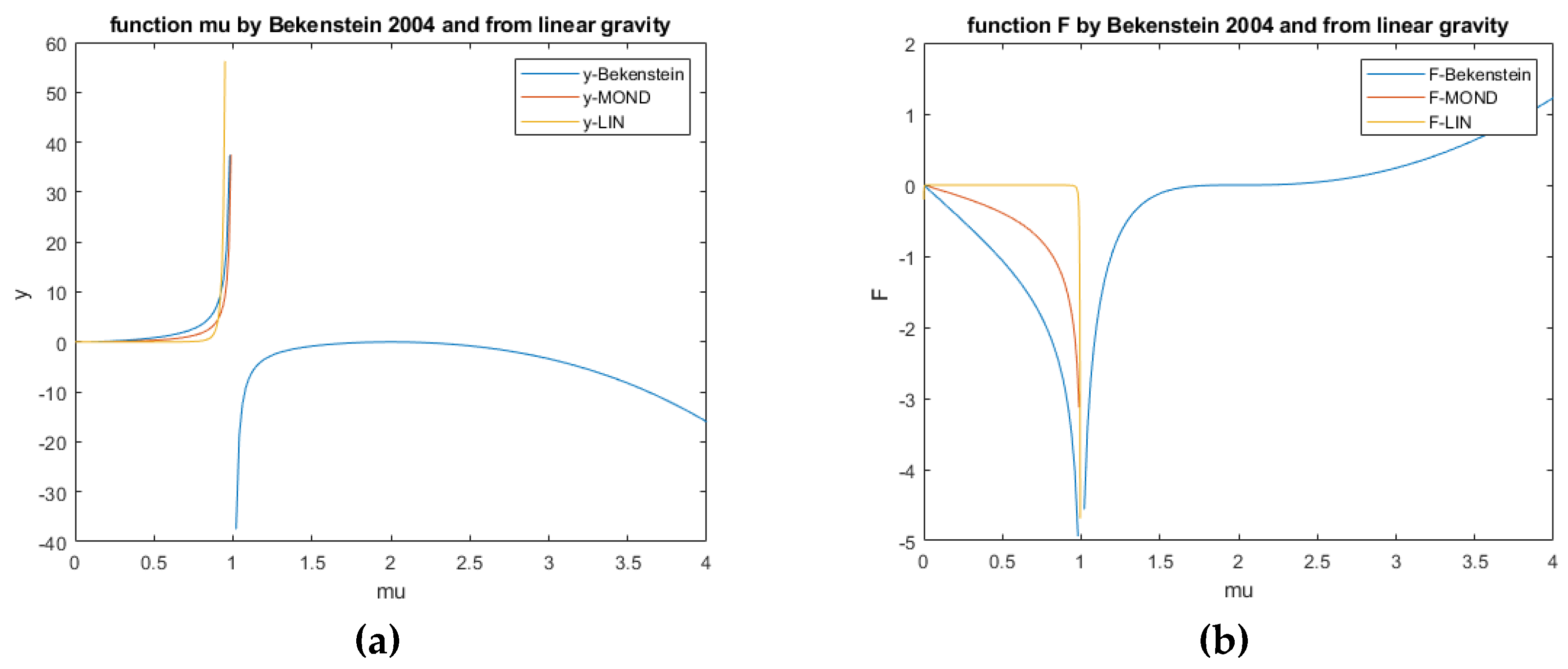
Figure 11a shows it gives a somewhat steeper increase towards µ = 1, but the trend as well as the sign and magnitude are of the same order as MOND and TeVeS. And no values for µ > 1 to account for cosmological effects are needed now, since dark matter is part of this hypothesis, opposed to MOND and TeVeS. The most left part, with µ << 1 is the deep MOND-regime. µ = 1 is the case where Newtonian gravity fully dominates.

However, c is not a constant but depends on the mass m_i in a certain position in the galaxy now as discussed in chapter 5.2 formula (20). But, on using a linearised metric as in Bekenstein [3] (p. 18, section B) the sum is a valid solution when each contribution to the sum is a valid solution. As explained by Bekenstein and for example in Schutz [41] (p. 200) this is valid for low gravitational acceleration where space-time is nearly flat.

So, in galaxies, y may be treated the sum of many contributions from all mass in the galaxy, each with their own value of c, i.e conforming to formula (20). c_i. And in galaxies with a bulge, in line with chapter 5.2, the bulge and the disk can be treated separately and the results added to yield a solution for the galaxy with bulge as a whole. The same applies to all different masses in a galaxy. So, if at one radial position R for one contribution from mass at another position X, agreement is proved, it is valid for the total acceleration g at a point.

Integration of (24) with use of (25), with c* = c⁴/a_m², gives:

$F\left(\mu \right)={\displaystyle \frac{2c^{\mathrm{*}}}{3{\left(\mu -1\right)}^3{\mu }^2}}+{\displaystyle \frac{k_1}{{\mu }^2}}$ (26)

k₁ is an integration constant, which can be chosen small compared to c* such that the function F(µ) at small values of µ, i.e. in the outer regions of the galaxy, is not dominated by the most right quadratic term in (26) but continues to converge steadily when µ, goes to zero. µ is limited to the range [0-1) in galaxies and when µ = 1 Newtonian acceleration is the only contribution to the acceleration, so in the centre of the galaxy and y would go to infinity. Bekenstein applies his function F to values of µ > 1 for cosmology and gravitational lensing, but that is not necessary if dark matter is used to explain those effects.

Again, as Figure 11b shows, the function F by linear gravity towards µ = 1 is steeper, but the trend and the sign are as well as the orders of magnitude are the same. The same applies to the function derived from MOND, what Bekenstein did not show, but is done here in the same way equation (26) was derived. As can be seen in Figure 11 in chapter 5.4 as well as Annex 3, the impact of the differences in F on the predicted rotation velocities are rather small. And again, no values for µ > 1 to account for cosmological effects are needed here.

This latter restriction, valid since dark matter is not excluded here, as well cures some of the reported problems of TeVeS like the incompatibility with the value of the quantity E_g at cosmological scales reported by Zhang [42]. Since linear gravity is an explanation of dark matter and not designed to do without it, the function µ, does not have to account for gravitational lensing effects and cosmological dark matter. Like in MOND, it only is applied in the range µ =[0-1), so with a positive contribution of dark matter to gravity. And since it is only applied for very weak fields, determining the motions of stars and gas in galaxies, the TeVeS problem with instability in stars reported by Seifert [43] does not apply here either. Applying TeVeS as a mathematical approach to dark matter is in line of the hybrid approach to dark matter as advocated by Banik [2].

5.4.2. Assessment of Evolution in Time with TeVeS

Bekenstein [3] also explores the dynamic, time-dependent, behaviour in his section E for, among other, the matter era in the evolution of our universe. Please note, the elaboration in the sequel fully applies to his theory and MOND as well, since in the outer regions of galaxies, i.e. the deep MOND regime, the theories behave the same with respect to the function y(µ), as can be seen upon comparing formulas (2) and (3) with (8) for small values of g, and the same for F(µ). And these functions are still free in Bekenstein’s scalar equation [3] (Bekenstein’s equation (37)) that is applied down here again.

Recall that µ is the ratio of Newtonian acceleration over total acceleration. Hence it is a decreasing function of the radial position in a galaxy and a supposed decay of the additional gravity by dark matter would make it grow towards unity. To explore this, Bekenstein uses the Friedmann-Robertson-Walker (FRW) cosmology [3] (p. 10) in which a(t) is the scale factor of the expanding universe.

$g_{\alpha \beta }d{x}^{\alpha }d{x}^{\beta }=-d{t}^2+a\left({t)}^2\right[d{\chi }^2+f\left(\chi {)}^2\right(d{\theta }^2+si{n}^2\theta d{\phi }^2\left)\right]$ (27)

Bekenstein uses (27) to a obtain a modified, now time-dependent scalar equation, (30) in the sequel, as well as a modified Friedmann equation (28) in TeVeS. Then he uses a combination of both to study the resulting evolution of F and ϕ, the additional gravitational potential caused by the added scalar field, in time.

His modified Friedmann equation, obtained from variation of his additional action S with respect to this metric, with ρ being the proper energy density and p the pressure and ϕ > 0, is:

$\left({{\displaystyle \frac{1da}{adt}}}^2\right)={\displaystyle \frac{8\pi G}{3}}\rho e^{-2\varphi }+{\displaystyle \frac{4\pi }{3k^2{l}^2}}⌊-\mu y\left(\mu \right)+{\displaystyle \frac{1}{2}}{\mu }^{2}F\left(\mu \right)⌋$ (28)

Please note, that all variables are scaled such way by Bekenstein that ϕ << 1 and that is it dimensionless [3] (pp. 8, 12 and 20). Later on he will argue that the left term of the right-hand-side in (28) dominates over the right term, which he then ignores.

Now Bekentein wants to find a relation between the time derivatives of a(t) and ϕ(t) by combining this, as said, with a time dependent scalar equation. Applying his scalar equation (Bekenstein’s formula (37)) to the FRW metric yields Bekenstein’s formula (45) copied down here [3] (p. 10):

$\mu \left(-2k{l}^2\left({d\varphi /dt)}^2\right)\right){\displaystyle \frac{d\varphi }{dt}}={\displaystyle \frac{-k}{2a^3}}{\int }_0^{t}G\left(\rho +3p\right)e^{-2\varphi }{a}^{3}dt$ (29)

Since the function F(µ) was part of the definitions of Bekenstein’s additional action S_s and hence of formula (23), the function µ reappears here as part of a differential equation, but, as mentioned earlier, with F still free.

In the matter era $p \approx 0$and ρ varies as a^-3 [3] (p. 21). Then integrating equation (29) from the start of this era gives:

${\displaystyle \frac{\mu d\varphi }{dt}}={\displaystyle \frac{-k}{2a^3}}{\int }_{t_r}^{t}G\rho e^{-2\varphi }{a}^{3}dt+{\displaystyle \frac{{\mu }_r{d\varphi }_r}{dt}}{\left({\displaystyle \frac{a_r}{a}}\right)}^3$ (30)

The time t_r is the time at the end of the radiation era and the start of the matter era, where a = a_r. Now Bekenstein explicitly evaluated this integral from t_r to t to let (30) become the following equation:

${\displaystyle \frac{\mu d\varphi }{dt}}={\displaystyle \frac{-1}{2}}kG\rho \left(t-t_r\right)+{\displaystyle \frac{{\mu }_r{d\varphi }_r}{dt}}{\left({\displaystyle \frac{a_r}{a}}\right)}^3$ (31)

Now equation (28) is used to express the left term in the right-hand-side in as a function of ${\displaystyle \frac{ 1 da}{a dt}}$.

After that, Bekenstein argues that after the start of the matter era, after the first e-folding of a, the first term of the right-hand side becomes dominant, so over most of the matter era up to the present. Ignoring the second term in the right hand makes (31) a simple differential equation. This is elaborated down here following Bekenstein.

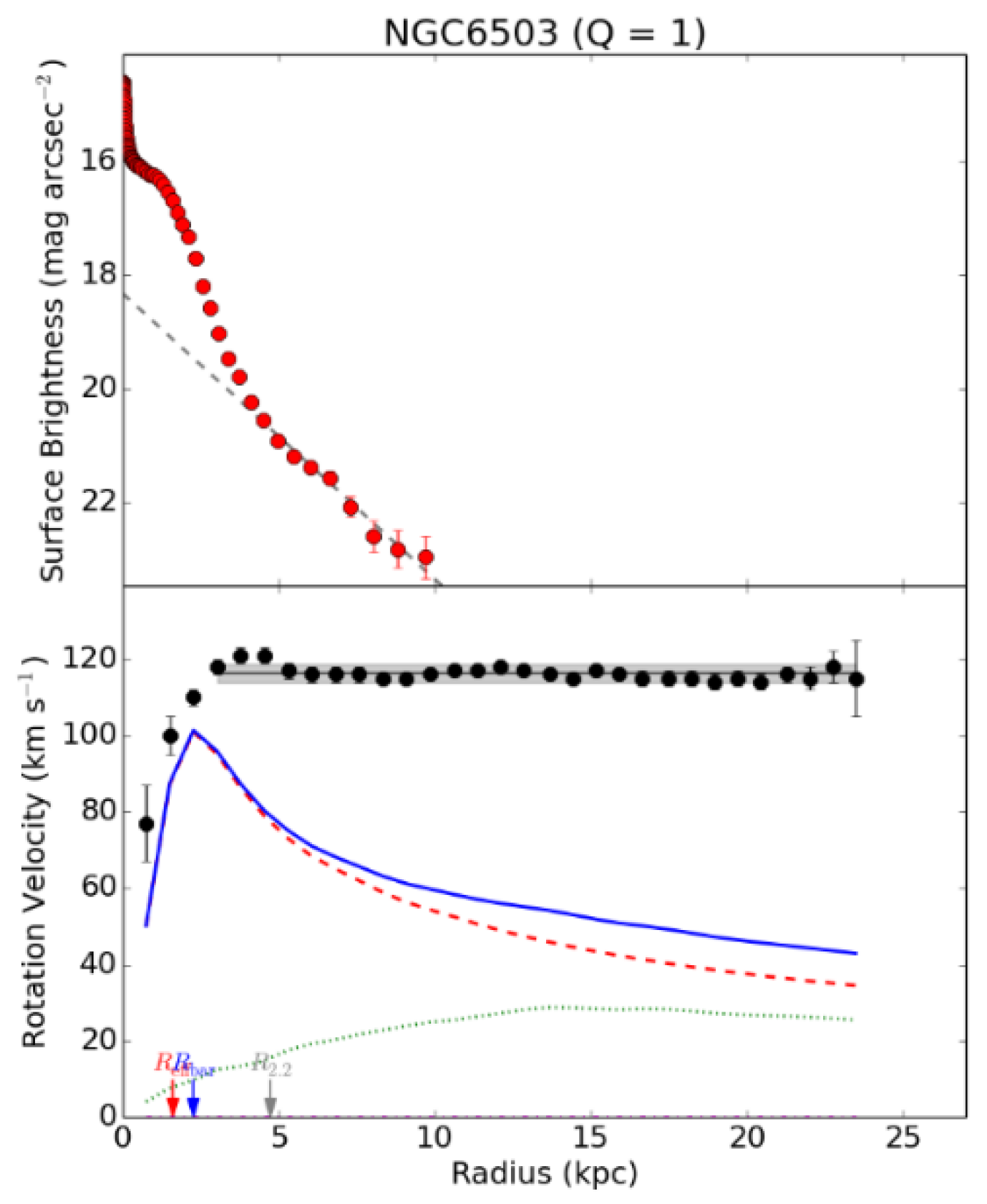
Bekenstein [3] (p. 22) only elaborates on the situation that µ > 2, so for application in cosmology and then states the evolution in time is small. But it is important to note that if µ << 1, like in the flat rotation region of a galaxy (typically in the order of O (0.1) in the 175 galaxies studied with a deep MOND regime) dϕ/dt might become very large indeed in this equation. For it then is multiplied with a very small µ in the left-hand side, which is relevant in the sight of the third prediction of this paper. So, this case is elaborated in the sequel.

Bekenstein does solve this equation with the help of (28) and ends with the following inequality, which in galaxies gets a < sign, since now F < 0 and y > 0:

${\displaystyle \frac{\mu d\varphi }{dt}}<\left({\displaystyle \frac{k}{8\pi }}\right)\left({\displaystyle \frac{\frac{da}{dt}}{a}}\right)$ (32)

But, he argues that this inequality is nearly saturated, since the scalar field contributions to his modified version of the Friedmann’s equations (28) are small compared to the left term in the right-hand-side [3] (pp. 20 and 21) as mentioned earlier after equation (28). Since in galaxies the absolute values of µ, y and F, are all smaller than in cosmology (µ > 2) this is even much truer in galaxies as can be seen upon comparing the left and right parts of Figure 8 with each other.

Then he integrates his equation from t_r to the current time t, But this can only be an approximation since µ actually is a function of time too, so this is valid only for a certain value of µ. With µ = O (0.1) instead of 2 this gives:

$\varphi \left(t\right)-{\varphi }_r\approx -\left({\displaystyle \frac{5.6k}{8\pi }}\right)\ln \left({\displaystyle \frac{a}{a_r}}\right)$ (33)

With k = 0.03 as determined by Bekenstein, it follows that this decay $\varphi \left(t\right)-{\varphi }_r$amounts to -0.11 approximately. In his work, Bekenstein [3] (pp. 20-22) scaled his variables such that during the entire cosmological evolution ϕ << 1 (i.e. e^ϕ≈ 1). His initial value was 0.007 < ϕ₀ << 1 [3] (p. 22). This simply means that the predicted decay of -0.11 in a typical galaxy, dominates the current value of the gravitational potential by linear gravity, so in the past it must have been much stronger than nowadays. Comparing Milgrom’s constant with Earth’s gravitational acceleration, confirms it is a very weak field nowadays in galaxies, so ϕ << 1 at present. Bekenstein [3] (pp. 10,11,12) gives another estimate of ϕ in cosmology and in localised systems like galaxies, and states that ϕ as defined in his theory nowadays typically has a value of order O (k). The actual value of order k = 0.03 evidently is much smaller than 0.11.

And for galaxies the inequality (32) gives an lower limit on the decay. Recalling it has a negative value, it’s magnitude may be larger even than 0.11, provided µ were constant, what is discussed in the sequel. And, as can be seen in equation (32), there will inevitably be a decay as long as there is linear gravity, except when k would be zero, but that would mean no linear gravity, so no dark matter.

But all this is only relevant when the decay of the additional potential affects the additional gravitational acceleration. So, the radial derivatives of the potential must be affected by this in a galaxy. µ being a decreasing function of the radial position, as stated earlier, ensures this. It decreases with increasing radial position and hence increases ${\displaystyle \frac{d\varphi }{dt}}$ as function of the radial position, cf. formulas (30) to (32). So the additional acceleration in a galaxy decreases as well. It must have undergone a vast decay since the start of the matter dominated era, since through the lower µ values then, ϕ varied much more with the radial position than it does now, so it’s radial derivative must have been huge compared to nowadays.

Consequently, the lower values of µ in the past made the magnitude of the decay much larger than 0.11 in the past. The decay getting smaller and smaller as time proceeds is exactly what you would expect for a dilution as described in chapter 5.3. This can be made explicit by solving (33) again, but now assuming µ is a function of time t as well, so as to check whether the predicted additional acceleration in the past as well decreased linearly with radial position, consistent with the hypothesis.

This can be checked by modifying equation (7) analogue to the approach leading to the FRW metric and see if the equation has a solution. Bekenstein follows exactly the same approach [3] p. 10) to obtain his equations (Bekenstein’s equations (44) and (45) and the text above his equation (44)). So equation (7) is modified as follows:

$\Phi ={\Phi }_N+f\left(t\right)\mathit{ln}\left(R\right)$ (34)

Then, differentiating (34) with respect to R gives a gravitational acceleration that is as well proportional to f(t). Hence, if one defines a function f(t) that decreases or increases the potential ϕ with time t, so that ϕ(t) = f(t-tr) ϕ_r, then it follows logically that µ(t) = f^-1(t-t_r) µ_r. In the sequel it will be verified this has a solution.

Inserting the above in equation (32) and as argued, considering (32) nearly saturated and assuming ${\displaystyle \frac{a}{a_r}}={\left({\displaystyle \frac{t}{t_r}}\right)}^{{\displaystyle \frac{2}{3}}}$ [3] (p. 21), [13] (p. 236) makes it a simple differential equation in f(t-tr). Rewriting this in terms of ${\displaystyle \frac{a}{a_r}}$ and solving it, makes it possible to extrapolate as well to the current era with accelerating expansion, where t_r in the denominator of the fraction can be ignored:

$f\left(t-t_r\right)={\left({\displaystyle \frac{a}{2a_r}}\right)}^{-c}$ (35)

With c = k/(8π ϕ_r µ_r). The exact speed of the decay is unknown, but clearly depends on the product ϕ_r µ_r. But ϕ_r and µ_r are unknown, and their values, at the start of the matter dominated era, cannot be determined directly from the current values using equation (36). For the galaxies have undergone an evolution in this long period. But it can be showed, the assumptions made up here, ϕ(t) = f(t-tr) ϕ_r etc_,, in this derivation, beneath equation (34), are not a limitation, since f(t) is eliminated in the product ϕ_rµ_r, for it appears in both the numerator and the denominator. And during the largest period of the matter dominated era galaxies as studied here did already exist, from 300 million years after the Big Bang [13] (p. 141), and before that the matter that would form the galaxies already existed in localised and rotating clouds of matter, so formula (33) may hold over the very largest part of this period [13] (p. 150).

Besides this, it can be shown, this as well holds when the most right term in the right-hand side of equation (30) is not ignored; then the right-hand side of (36) only will be multiplied with a power of e, that in the product ϕ_r µ_r still drops out. But the current value of the product ϕ µ clearly is not a constant, and will be a function of radial position R in a galaxy, so it does not have a unique value now, but it does not vary with an order of magnitude, since it varies only with ln(R)/R (less than a factor 8 from 2 to even 100 kpc). Given this small range, the deviation from the assumptions made in equation (34) in the first period of this era may be limited. So, using actual values, some constraints and an estimation can be given to find the order of magnitude of c.

A constraint on µ_r for c to be unity, so the power of a/a_r is minus unity, i.e. the most simple form of a dilution of ϕ from galaxies, can be derived. Given the lowest value for ϕ_r estimated in the above ϕ_r > 0.11, the value of c could be unity when µ_r < 0.012. This is realistic when compared with the current typical value of µ = O (0.1), and a pair of values for ϕ and µ that obeys to this and to equation (37) can exist. And, as mentioned, Bekenstein [3] (pp. 10,11,12) gives an estimate of ϕ in cosmology and in localised systems like galaxies, and states that ϕ as defined in his theory currently typically has a value of order O (k). Combining this with the current typical value of µ = O (0.1) in the deep MOND regime, gives an estimate of the order of magnitude of the power: c = O (1). So the dilution of ϕ from galaxies, and hence the growth of µ, goes with a power of a/a_r that is of order O (-1). So, the power law (35) indeed is typical for a case of simple dilution of a physical quantity with the scale of space a.

To summarize: since the function F was part of the definition of Bekenstein’s additional action S_s and hence of formula (23), the function µ reappears as part of a differential equation for ϕ(t) when Bekenstein’s actions are combined with the, time-dependent, FRW metric. It is shown there is a decay of the additional gravitational potential by linear gravity with time, that the decay till now has been vast, that it follows a power law typical for simple dilution of a physical quantity with time and that the power has a value in the order of minus unity. The increase of µ in time, per definition would mean a decrease of Milgrom’s constant a_m in time. Sanders [44] with the assumption of a constant a_m already showed that MOND predicts faster development of structure in the early universe and the decrease of a_m in time will make this effect even stronger. This all confirms the third prediction of this paper and this significant time evolution of ϕ in TeVeS gives an even more powerful explanation for the rapid evolution of large galaxies in the early universe.

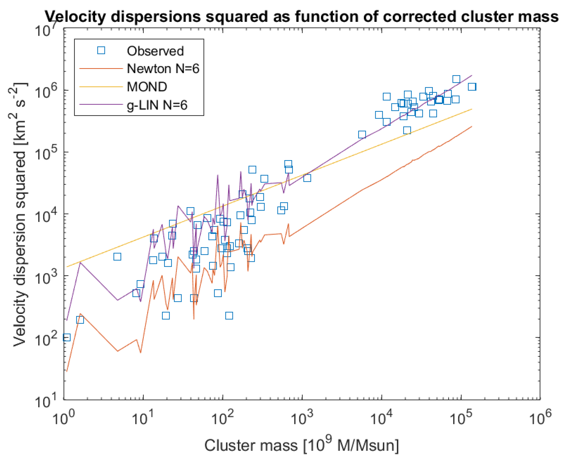
5.4.3 Strong Support for an Evolution in Time from Galaxy Clusters

Strong support for the predicted evolution in time comes from galaxy clusters. It will be shown the linear mass density here is vital to be able to significantly improve the predictions of the velocity dispersions. The clusters show velocity dispersions that depend on the gravitational potential and obey the Virial theorem, see Milgrom 2018 [45]. Milgrom used data from NGC clusters only, but Tian, McGaugh et al in 2021 [46] analyzed the much larger Abell clusters as well. The data of both sources have been combined in the graph down here in Figure 12.

The Newtonian, and the MOND approach, as well as linear gravity will be elaborated and used to predict the dispersion velocities from the mass M and the diameter R_h of the clusters.

The Virial theorem states that if a spherical distribution of objects of equal mass is stable and self-gravitating (such as a galaxy cluster), the total gravitational potential energy, U, of the objects is equal to minus two times the total kinetic energy, T:

$2T+ U= 0$ (36)

With U being the sum of all the dot products of the gravitational forces acting on test masses and the vectors to the mass center as follows:

$U=\sum _i\overrightarrow{F_i}.\overrightarrow{r_i}$ (37)

With Newtonian gravity and with the commonly assumed ratio of 3 between the velocity dispersion and the line-of-sight velocity, that is the measured quantity, the following equation results for the line-of-sight velocity dispersions σ, after Heisler et al in 1985 [47]:

${\sigma }^2={\displaystyle \frac{\pi GM}{32R_h}}$ (38)

But, Milgrom has applied the Virial theorem to the MOND formula (5) for spherical clusters in Milgrom [45]. For linear gravity it is simple to derive a comparable formulation from this, what will be done in the sequel. Milgrom’s formula for the dispersion velocity in a cluster is:

${\sigma }^2=\sqrt{{\displaystyle \frac{GM{a}_m}{9}}}$ (39)

Since G and M and a_m are just constants for a given cluster, for MOND works on the resulting gravitational acceleration from all the different masses on a test mass (and not on the separate contributions, so the square root in the next only applies to the sum), they can very well be replaced by another constant without changing the steps taken in the derivation by Milgrom [45]. This will be done here. In the deep MOND regime the gravitational acceleration in a galaxy is $g= \sqrt{G M a_m}/R$, whereas in the linear gravity formulation (10) for N superposed masses this is g = 2*N*G_LM’/R, since the potential energies of N times the visible mass add up, so this leads to:

${\sigma }^2={\displaystyle \frac{2N{G}_{L}M\mathrm{\text{'}}}{3}}$ (40)

However, so as to compare this with the said NGC and Abell data, the average linear mass density has to be expressed in the mass of the entire spherical cluster, so using M instead of M’, which is straightforward, since the average mass density of an 2-dimensional cross section, with average radius, through a sphere with uniform mass amounts $M\text{'} = M/ R$. Inserting this in (40) gives:

${\sigma }^2={\displaystyle \frac{{2NG}_{L}M}{3R}}$ (41)

Which closely resembles the Newtonian result (38), despite the fact that (41) was derived using MOND (!), so results from a logarithmic potential.

But this can as well be derived in a direct manner from the Virial theorem using the logarithmic potential of N times a hypothetical 2- dimensional disk that is consistent with linear gravity from formula (10), and down here it will be shown this gives the same result.

The total potential energy of the mass in a cluster U was formulated in equation (37) and with the potential (10) the Virial theorem from formula (36) yields:

$2T-\sum _i\sum _j{\displaystyle \frac{2Nd{M}^{\mathrm{\text{'}}}\mathit{ln}\left(\left|r_{ij}\right|\right)}{d\overrightarrow{r_{ij}}}}.\overrightarrow{r_{ij}}=0$ (42)

Now, since in a line mass the vectors $\overrightarrow{r_{ij}}$ just point perpendicular to the line mass, taking the dot product is the same as multiplying with this distances $r_{ij}$, and differentiating the logarithm leads to the same distance $r_{ij}$ in the denominator. So, this is canceled. And that, again with ratio of 3 between the velocity dispersion and the line-of-sight velocity, leads to:

${\sigma }^2={\displaystyle \frac{{2NG}_L{M}^{\mathrm{\text{'}}}}{3}}$ (43)

Which results in the same as formula (40) that was derived from MOND. So, again, this formula closely resembles the result that follows from Newtonian gravity (38), with the same slope, but giving higher velocity dispersions as will be argued in the sequel. This is astonishing, since a logarithmic potential as in MOND in a spherical cluster leads to squared dispersion velocities that are proportional to the square root of M in formula (39) and linear gravity, which as well has a logarithmic potential, ends up with a very Newtonian-like result.

However, both said literature sources, as well as Banik [2] reveal that when the Virial theorem is applied to the Newtonian potential, see formula (38) this needs significantly more mass than the visible to match the observed velocity dispersions. In conventional cosmology it is assumed the dark matter amounts to approximately six times the baryonic matter, but this does not suffice to bridge the gap, as is well shown in Tian, McGaugh et al [46] This factor six has been applied to the data in the graph in Figure 12 down here to yield the Newtonian velocity dispersions including the effect of dark matter. And, contrary to Milgrom’s findings for smaller and nearer by clusters (Milgrom 2018), the full range including the Abell clusters, reveals the MOND data are significantly lower than the observations in the Abell clusters and the corresponding curve in Figure 12 does not have the right slope.

But, the paper in hand proposes a hybrid approach, in which the existence of dark matter is included. Therefore, in line with the Newtonian approach of conventional cosmology, much dark matter can be resident in the clusters, even much more than in the galaxies alone.

The theory in hand suggests this is dark matter diluted from the galaxies into the space between them. So, the essential idea here is the dark matter diluted from galaxies will still be in the clusters now. To give the best fit with the observations, an additional factor 104 has been assumed for this ratio. This means in this hybrid approach there is much more dark matter in the clusters than the dark matter that diluted from the galaxies only, which is credible. Now, the fundamental clue of all this is that this additional factor 104 exactly matches the ratio of G_L/ G found in galaxies in chapter 5.3, assuming the number of superpositions N = 6, which was in line with the ratio of dark matter and baryonic matter in conventional cosmology!

In line with the elaboration at the start of this chapter, it is predicted dark matter diluted from the galaxies because of the expansion of space and hence the appearance of new space between the 2-dimensional cross sections of the universes. But, from the Nasa/Ipac Extragalactic Database it can be deduced the farthest Abell clusters are at a distance of approximately 1 Billion lightyears from ourselves, what corresponds with an expansion of space-time of approximately 2.5 % in that period of time, which is insufficient to give the effect visible in Figure 12. But the factor 104 does.

This gives a reduction of the r.m.s. of the deviations from the observations of 44 % compared with both MOND and 57 % compared with the conventional Newtonian approach, see Table 2.

The said additional factor of 104 on the amount of dark matter needed in clusters compared to that in the galaxies alone, is consistent with the hybrid approach of this paper in hand. The number of superposed universes, N, that lead to all this dark matter will be discussed in the next section. Given the ratio of G_L/ G of approximately 104, it must be N = 6. See the next section. Roughly the same value will be derived in another way the sequel.

5.4.3. Further Support for an Evolution in Time

Recently a paper published in Nature by Labbé et al. [48] confirmed this evolution in time. The James Webb telescope showed there is a very rapid development of large galaxies already at 600 million years after the Big Bang [48]. Following Heuvel [13] (p. 236), the diameter of the universe over this timespan expands with time^2/3. Thus, the diameter of our universe was roughly 7 times smaller than now. As a result, linear gravity according to our hypothesis was significantly stronger too.

This rapid development of large galaxies is much sooner than the current theories predict. But a much larger gravitational acceleration can account for this, since that will greatly accelerate the contraction of gas clouds and the development of stars and galaxies, as discussed by Sanders [44] and McGaugh [49].

Another prediction, that logically follow from this, is that because of this extra gravity, the rotation velocities of these early galaxies will be shown to be exceedingly higher than what we observe in nearby galaxies. This prediction can eventually be assessed.

The question remains to what extent this can be extrapolated back in time into the smaller universe that existed then. Looking back in time, the ratio of linear gravity over Newtonian will not increase anymore when the distances over which it can work at all, start to decrease as well. This was roughly the case before the moment that all 2 Billion galaxies in clusters and the filaments of the cosmic web, see Conselice, 2016 [50] would be packed together. This was when the volume of the universe would be 5 x 10^-8 the current value. From that moment back in time the density of dark matter will continue to increase when looking back into the past, but the square distance term in the Newtonian gravity will increase more rapidly than the linear one, so the ratio of Newtonian and linear gravity would not change anymore when looking back. This perfectly compensates each other at the smallest sizes of our universe in the far past. Besides this, the thickness d in the mass density formulation M’ = M/d will decrease too when all the clusters and filaments will be compressed in a smaller volume than the said 5 x 10^-8 times the current value. This will make it such that the value of the constant G_L did not vary in earlier times! Now, for the volume to be reduced to the said 5 x 10^-8 times the current value, the radius of the universe must have decreased by a factor 260. But, this is nearly the same ratio as the factor 104 for G_L /G mentioned up here. In fact, the power c from formula (35) in section 5.3.2 should be 0.8 approximately to make it match, which is consistent with the order of O (1) mentioned there.

But, even more direct support for the predicted dilution now comes from the value of the linear gravitational constant that will be derived in the next section from the SPARC database and that amounts to G_L ≈ 6.64 x 10^-13 [m³ kg^-1 s^-2]. As said, this is approximately 104 times smaller than Newton’s gravitational constant, though it has the same dimension and the same meaning. As said, conventional cosmology suggests there is even six times more dark matter than baryonic matter, which is as well allowed by the theory in hand. This suggests that the additional gravitational potential is diluted 104 times since the moment in the past where the distances over which it can work decreased as well, when looking further back, as mentioned up here. Despite the fact that this is higher than the 36 times calculated with TeVeS in the previous section, it is of the same order of magnitude and the power to be used in the previous section remains the same order of magnitude. The clusters would lead to a value 0.8 instead of 0.4, so still O (1), still signifying a simple dilution.

5.5. Fifth Prediction

A fifth prediction is that the dark matter is undetectable in any way, since it cannot interact with visible matter, except by gravity, which deforms space and time. In chapter 4 it is argued that electromagnetic waves cannot propagate in and through the 2-dimensional intersections of overlapping universes in the superposition state. The effect of this non-interacting is directly visible in the Bullet cluster [13]. By calculating the distribution of dark matter, the researchers have shown the dark matter acts like visible matter and just flows through the other galaxy, because of its momentum, whereas the ionized HI gas cloud, interacts and stays behind. If the halos were to be recomputed based upon the linear gravity proposal, this behaviour might still be visible in the Bullet Cluster.

Now, according to the hypothesis in hand, there is another fundamental reason why dark matter is undetectable. That is orthogonality, see Griffiths & Schroeter [16] (p. 98 and 151) in terms of quantum mechanics. It follows from the definition of a superposition state, namely as a linear combination of independent quantum states, i.e. orthogonal states. They are per definition not accessible to each other. For the superposition of 3-dimensional universes in a 4-dimensioanl space with two overlapping dimensions, the meaning of this is evident, because one of the dimensions is orthogonal to that of the other universes. But it is in all cases necessary to maintain a superposed state. For instance, Zeilinger [51] states about the double-slit experiment: “The superposition of amplitudes .. is only valid if there is no way to know, even in principle, which path the particle took. It is important to realize that this does not imply that an observer actually takes note of what happens. It is sufficient to destroy the interference pattern, if the path information is accessible in principle from the experiment or even if it is dispersed in the environment and beyond any technical possibility to be recovered, but in principle still ‘‘out there.’’ The absence of any such information is the essential criterion for quantum interference to appear”.

That is why we can never perform any measurement on the properties of dark matter. This information must be and remain absent for the superposition at the earliest stage of the Big Bang to have been possible at all.

5.6. Sixth Prediction

As mentioned in chapter 4, Han [32] shows that the Milky Way galactic stellar halo is tilted with respect to the disk plane, suggesting that at least some component of the dark matter halo may also be tilted. The origin of this misalignment of the dark halo, of approximately 25°, can be explained by the linear gravity hypothesis in the paper in hand, since the orientation of the two dimensions of another superposition state overlapping with ours, can deviate from the orientation of a galaxy and can be anisotropic if the amounts of matter in overlapping galaxies differ. The sixth prediction is that the orientations of the halos of different galaxies will reveal a deep underlying structure in the universe, i.e. will display the direction of the pair of two dimensions overlapping with our universe. In other words, the orientations of the halos will, when compared with each other on a large scale, display the underlying coordinate system, of sorts, of the universe.

6. Conclusions and Suggestions for Further Work

The hypothesis of dark matter is a way to explain why among other galaxies seem not to obey Newton’s law of gravity. As well, dark matter is needed to explain the statistical distribution of ‘cold’ and ‘hot’ spots in the background radiation, that would still need the existence of (much) dark matter vs. baryonic matter to be understandable in terms of Big Bang nucleosynthesis, as well as matters like gravitational lensing and gravity in galaxy clusters. Alternative approaches like MOND and TeVeS work well to describe the flat rotation curves in galaxies as such, but do not give a natural explanation for the concepts and additional fields they introduce. In this paper, as recommended by Banik in Symmetry, a hybrid approach to dark matter is presented, in which Bekensteins TeVeS is applied as well, but only as a mathematical tool to describe gravity. But, it should be insisted, the existence of dark matter is taken as a starting point in this article. A natural explanation for the nature of dark matter is presented based upon Hawking’s cosmology and String theory that has its foundations in it.

The conclusion is that the universe consists of four 3-dimensional universes, existing as at least four states of a superposed 4-dimensional multiverse, which each have two overlapping dimensions with the observed universe. For there is nothing outside it that could disturb the superposition state, it could be in that state forever, without de-coherence effects ending it. That is why Hawking and others can speak of the wave function of the universe in the first place.

The superposition leads to the existence of additional baryonic matter, but in superposed universes and hence ‘dark’, with gravity that attracts matter in other superposed universes through the 2-dimensional intersections. The 2-dimensionality of the intersections explains both why the additional gravitational acceleration decreases linearly with distance and why electromagnetic waves cannot propagate through it. And this, together with the orthogonality of superposition states, gives a natural explanation for dark matter particles being undetectable.

Gravity from dark matter and visible matter is very well interpreted as the sum of two gravitational accelerations. Modelling dark matter as a set of three orthogonal line masses with the Levi-Civita metric and adding this to the Schwarzschild metric for a baryonic point mass, gives a valid solution of the Einstein field equations in the weak fields that occur in the galaxies studied and directly leads to the Tully-Fisher relation.

In each galaxy, one constant value for the ratio between the surplus acceleration and the sum of all mass-density over distance can be determined. This will be called the ‘linear constant of gravity’, G_L. From the values of the calculated baryonic and the observed velocities in galaxies in the SPARC data, an average value for the gravitational constant G_l of the 2-dimensional gravity is deduced: G_L ≈ 6.64 ± 0.02 x 10^-13 [m³ kg^-1 s^-2]. This is not a fine-tuned number as meant in Hossenfelder [10], but an empirical value that represents the average effect of the matter in the superposed universes as observed in our galaxies. The amount of matter in the galaxies in the superposed universes can vary according to their history, which becomes visible in the values of G_L that vary from galaxy to galaxy. But this value proved to give a much improved prediction of dispersion velocities in galaxy clusters.

The mass-to-light ratio has been used as the only fitting parameter to fit the baryonic rotation velocity, and hence the baryonic gravitational acceleration in each galaxy to the observed values near the core of the galaxies. After that, the above-mentioned value for G_L is used to predict the additional gravitational acceleration at all radii without any further fitting. Applying this value to predict rotation velocities from the baryonic matter distribution in a galaxy, upon using the mass density in the plane of rotation, will yield predictions that are on average 10 to 17 % closer to observation than MOND or Bekenstein’s work, TeVeS. With 175 dedicated values of G_L, this improves further to 19 to 27 %. In galaxy clusters, the improvement of the predictions of the velocity dispersions is even much more.

Further investigation of the shapes and orientations of dark matter halos based upon the linear gravity hypothesis, will yield line-masses with comparable orientation as the ones currently calculated by many researchers, but much more concentrated at the centre of galaxies. This avoids the fundamental problems with the current view of halos surrounding galaxies as recently reported by Mistele and Lelli based upon the SPARC data.

Using the work of Levi-Civita and Santos it is shown a consistent relativistic formulation of the hypothesis can be constructed in GR. As an alternative approach, the work of Bekenstein has been elaborated too to study the evolution in time of linear gravity. In the latter case this has been done following the same steps Bekenstein took with MOND and GR. The solution based upon TeVeS and the FRW metric confirms the prediction of decaying linear gravity from a decreasing concentration of dark matter in time, by the expansion of space in accordance with the hypothesis. But then, it becomes clear that somewhere in the past linearised calculations will break down, since then the field was much stronger and numerical approaches are needed. And, perhaps, the said models of Mistele and Lelli used to analyse the SPARC data are accurate enough to falsify or confirm the predicted decay, taking into account the evolution of galaxies in time. And, to check whether G_L stays constant over the huge distances, out to 1 Mpc, they analysed.

More future work is to implement the linear gravity approach, including the predicted evolution in time, in existing simulation software for the evolution of galaxies to verify whether that will yield better agreement with the observed trends, in particular the rapid evolution of large galaxies in the early universe as well as to study how linear gravity can be applied to gravitational lensing, including dark matter as a source.

The author looks forward to receiving responses to this hypothesis from the field.