
Submitted:
13 November 2024
Posted:
15 November 2024
You are already at the latest version
Abstract
This paper presents a varying-parameter finite-time recurrent neural network, called varying-factor finite-time recurrent-neural-network(VFFTNN), which is able to solve the solution of the time-varying Sylvester equation online. The proposed neural network makes the matrix coefficients vary with time and can achieve convergence in a finite time. Apart from this, the performance of the network is better than traditional networks in terms of robustness. It is theoretically proved that the proposed neural network has super exponential convergence performance. Simulation results demonstrate that this neural network has faster convergence speed and better robustness than the return to zero neural networks, and can effectively track the theoretical solution of the time-varying Sylvester equation.
Keywords:
Recurrent neural networks(RNN)
; finite time
; super-exponential convergence rate
1. Introduction
As we all know, the Sylvester equation , as a kind of linear matrix equation, plays an crucial role in many fields,especially linear algebra and matrix theory. For some mathematics, dynamic control system, and computer vision problems, Sylvester equation can be used to solve them, like designing the feedback control system by pole assignment optimization, linear least-squares regression, image fusion [1], clustering [2,3], and so on. In recent years, there exist many methods proposed by other scholars to solve real-time linear algebra problems [4,5,6,7,8,9,10,11,12,13,14,15,16,17,18,19].Among these methods, several methods are efficient and representative, like GNN methods and ZNN methods. It is notable that GNN and ZNN methods both use the thought to force the time derivative of the error function declining and further to force the error function gain on zero. The proposal of GNNs, as a emblematic recurrent neural network, is very representational for solving real-time linear algebra problems[20,21,22].Generally speaking, different GNNs are designed to solve different linear algebra problems. By itself, for solving the Sylvester equation, GNN methods are able to roughly stated as follows:
- 1)
- The first step, the error function is defined as . In order to acquire the solution of Sylvester equation, the error function should converge to zero.
- 2)
- In the next step, for purpose of acquiring the minimum point of the error function, GNN methods use a negative gradient descent direction. In addition to this, GNN methods employ a constant scalar-type parameter, which parameter is accelerating the convergence rate of the error function so that solving Sylvester equation efficiently.
However, GNN cannot track the ideal solution for the time-varying Sylvester equation well, because the GNN method is a kind of gradient-based method, which may makes the error definition of GNN unable to converge to 0 [23].Therefore, GNN cannot solve the Sylvester function with time-varying effectively. But in practice, time-varying problems are everywhere, so we need a neural network to better track solutions locus to time-varying issues in real-time. Under this background, many kinds of neural networks have been proposed to solve this kind of time-varying algebraic problems. Among these neural networks, the ZNN proposed by Zhang proved to be efficient[17].ZNN is a kind of implicit dynamic neural network, that skillfully replaces the gradient dynamic with implicit dynamic, so that the computation error can achieve better convergence, that is, with the increase of time, the solution of the network can approach the theoretical solution in real time[24,25,26,27,28,29,30,31,32].However, ZNN also has some shortcomings, such as its convergence speed is not fast enough, convergence parameters are difficult to set, and other issues. Aiming at the above shortcomings, Li proposed a finite time ZNN [24]. The sign-bi-power activation function has been used in this network, as effectively activates this network, makes the convergence speed much faster and can achieve finite-time convergence. In addition, Zhang proposed a variable parameter convergence differential neural network (VP-CDNN)[33]. Different from the initial ZNN, the convergence parameter of VP-CDNN change with time, which makes the network hardware implementation much more reasonable than ZNN, and the convergence speed has reached the super-exponential convergence speed. But despite this, VP-CDNN cannot achieve finite-time convergence. Based on the above discussion, this paper proposes a recurrent neural network (VFFTNN) for solving the time-varying Sylvester equation. The network not only has the speed of super-exponential convergence but also can achieve finite-time convergence.
The rest of this paper is divided into four parts. The second section introduces some tools needed to solve the Sylvester equation, and briefly describes the solution steps of ZNN. In the third section, the implicit dynamic equation of the proposed VFFTNN and the general steps of solving time-varying problems with the network are given, and the convergence and robustness of VFFTNN under different conditions are analyzed theoretically. In the fourth section, the simulation results of MATLAB are given and compared with the simulation results of ZNN. In the last section, the thesis is summarized.
Before concluding this section, some highlights of the paper are listed below:
- 1)
- Propose a VFFTNN algorithm for solving the Sylvester equation;
- 2)
- Compared with VP-CDNN, this network can achieve finite-time convergence;
- 3)
- Theoretically proved the convergence time of the network in the case of three activation functions;
- 4)
- In the situation considering the existence of disturbances, the robustness of VFFTNN is discussed;
- 5)
- Data simulation results show that the proposed VFFTNN has better convergence and robustness than the traditional ZNN model under the same initial conditions.
2. Problem Formulation And Prepare Knowledge
Let us observe the following Sylvester equation with smooth time-varying expressed as:
where time is expressed as the variable t. The time-varying smooth coefficient matrices , as well as . Besides, d/dt, d/dt, and d/dt are their time derivative respectively and assuming these time derivatives are known or can be found exactly. Furthermore, is uncharted but real, and our purpose is to find it so that to approach or even equal the unique ideal solution in finite time for the above Sylvester equation.
In order to facilitate the subsequent discussion and to solve equation (1) more simply, (1) is best to be transformed into a vector form. So the next Theorem (1) is introduced.
Theorem 1.
The Sylvester’s equation in matrix form (i.e., equation (1)) can be transform into the vector form as following:
where , as well as , represent n-dimensional as well as m-dimensional identity matrices, respectively. Besides, the symbol T represents the transpose of the matrix. The symbol ⊗ represents the Kronecker product. In other words, represents one large matrix, which is equivalent to turning the row and column position element in the matrix U into a matrix . Operate represents a column vector that puts totally of the columns of the matrix in sequence.
Proof.
See Section II as well as [17, Appendix]. □
Furthermore, if we want to obtain the only solution of equation (1), then it must meet the regularity condition [17,34], which is described in the following Theorem (2).
Theorem 2.
If the Sylvester equation (1) satisfies the following regularity condition, then it has one and only one solution.
where represents mn-dimensional identity matrix.
Proof.
See Section II and [17, Appendix]. □
With the continuous development of neural dynamics and the proposal of ZNNs, the idea of ZNNs is employed in many engineering and scientific fields to solve time-varying problems. For showing the details of this paper more clearly, next, we will briefly introduce how to solve the Sylvester equation (1) using a typical ZNN method.
In the first step,an error function about equation (1) is defined as follows:
Next, since our goal is to get a unique solution to equation(1), then when we set the error function approach 0, the unique solution of equation(1) will be acquired naturally. In the light of the design idea of neurodynamics, the following differential equations about the error function could be designed :
where the scale-valued factor is a positive design constant (i.e., ), which can adjust the convergence velocity of this network(5) through vary its value. is an array including the same activation functions. can be different kinds of activation functions, like linear-type, bipolar-sigmoid-type, power-type, sign-bi-power-type and so on. When we use the activation function with linear-type, (5) is a typical ZNN.
Based on (5), we can acquire the following implicit dynamic equation:
where the starting value of is . Besides, the state matrix is an approximate solution that will gradually approach the theoretical solution, and it will approach to only one solution of . In the light of the following lemma [17], the ZNNs performance to solve Sylvester equation can be guaranteed to exponential convergence.
Lemma 1.
Considering Sylvester-equation (1), its time-varying coefficient matrices , and , assuming that they satisfy inequality (3), and the activation function of the implicit dynamic equation (6) is chosen to be linear, then its state matrix will be exponential convergence from any original state to the time-varying ideal solution of (1).
3. Varying-Factor Finite-Time Recurrent Neural Networks
ZNN can achieve better convergence performance by means of using different activation functions or setting a larger constant factor [35], but its convergence performance still has room for further improvement. Inspired by classic ZNN design ideas, a novel recurrent neural network is put forward in this paper. It can realize a neural network with super-exponential convergence in a limited time, and because the factor before its activation function changes with time, it is called VFFTNN. It could be expressed as
where is a function about t, and it can be set to different functions. Here, for simplicity, we use exponential time-varying parameters , and is a positive scalar-valued factor, i.e., , and the positive scalar-valued factor , where s and q both are odd numbers. In the light of (7), we can reformulate its implicit dynamic equation form:
In addition, in the light of Theorem 1 and equation (2) in Section I, we are able to obtain the vector form of the above implicit dynamic equation (8):
where is a matrix, is a vector,and is a activation function array. It is notable that the transformation dimensions of in (9) are different with (5). The block diagram of VFFTNN can be drawn in the light of the implicit dynamic equation (8). As shown in Figure 1, ∫ and ∑ represent the integrator and accumulator respectively. The symbols L and R represent left and right multiplication of matrices, severally.
3.1. Convergence Analysis
The following theorem will lay the foundation which will come into play later when discussing VFFTNN global convergence.
Theorem 3.
For the time-varying Sylvester equation (1), its coefficient matrices , , and have been given. If equation (1) satisfies inequality (3), and the activation function sequence is opted to be monotonous and oddly increasing, then the state matrix of the VFFTNN model (8) can be global convergence from any original state to the time-varying ideal solution of Sylvester equation (1).
Proof.
First, we can convert VFFTNN system (7) into scalar form as
where represents the the row and column position element on . In addition the represents the activation subfunction of matrix elements.
Next, we will proof its global convergence. Let us define a Lyapunov function as shown below:
according to the above, we can calculate its derivative in time:
It can be seen from the previous definition that and is monotonous and oddly increasing. So for arbitrary and , we have
In the light of Lyapunov stability theory, error function (10) is global asymptotical convergent. Therefore for any, i and j in the domain, the error function in scalar form will asymptotically converge to zero. In other words, the online solution by using VFFTNN will approach its theoretical solution when .
In a word, the proof about Theorem 3 has been completed. That is, VFFTNN has global asymptotic convergence. □
In the next step, we will demonstrate finite-time convergence of VFFTNN under various activation functions (i.e., linear, bipolar-sigmoid, and power functions). See the following theorem for the specific convergence time.
Theorem 4.
For the time-varying Sylvester equation (1), its coefficient matrices , and have been given. If equation (1) satisfies the regularity condition (3) and the activation function sequence is monotonous and oddly increasing, then the VFFTNN system (8) can converge to the theoretical solution of equation ( 1) in finite time from an arbitrary original state. In addition, the specific convergence time of neural system in the cases of different activation functions is:
- 1)
- When we choose the linear activation function (i.e., ), the convergence time of VFFTNN .
- 2)
- When we choose the bipolar-sigmoid activation function (i.e., , ), the convergence time of VFFTNN .
- 3)
- When we choose the power activation function (i.e., , and s is an odd number), the convergence time of VFFTNN .
The above , and is respectively
where represents .
Proof.
In the following, we will prove the convergence time of the VFFTNN system under three different activation functions one by one.
- 1)
-
In the light of the differential function theory [35], we can acquire the solution of (13).where . Let in (13) be equal to zero, we can acquire the following:then we can easily find . In other words, for any i and j on the definitional domain, we have when , the scalar value . Note the definition of above, at this time, the error function in the form of a matrix will also approach zero, which means that the convergence of state matrix is guaranteed.
To sum up, we can acquire the convergence time when VFFTNN system has used the linear-type activation function as follow:
where . It shows that in the case where the activation function is linear, VFFTNN method can achieve finite time convergence in the problem solving Sylvester equation.
- 2)
-
Bipolar-Sigmoid-Type: In this situation, we can easily know that the activation function form is where and are scalar factors. So the following equation can be obtained from (10).where , . In the light of relevant knowledge of the differential theory, we can rewritten (15) aswhere . According to the Lyapunov function of this system, we can know that increases or decreases monotonically with the increase of t. So for simplicity, next we will only discuss the case of . Then we can acquire the followingAt this time we consider the following two situations.
- a.
- When , noticing that and are convex, solving for (16) can acquirewhere is a constant, determined by the scalar factor . Similar to linear-type, solve for (17), we can acquire
- b.
-
Notice that and are monotonically increasing over the interval , so when , and . Therefor, we have
- 3)
-
Power-Type: For power-type case, we can easily know that the activation function form is , where s is an odd number and . So the following equation can be obtained from (10).Similar to (16), we haveThe discussion is divided into the following two situations:
- a.
-
When , it can be found easily that , so . In the light of (24), we can acquireThen the result (25) can be acquired
- b.
-
When , we know that for all , we have . So similarly:Then the follwing result (26) can be acquired
In conclusion, when or , the scalar value for any i and j on the definitional domain.It means that the convergence of state matrix is guaranteed. The convergence time of the power-type can be represented as
In the light of the above analysis, it can be find that VFFTNN can achieve finite time convergence on the problem to solve Sylvester equation (1), no matter which of the three activation functions is used. So the proof of the finite time convergence Theorem 4 is completed. □
Remark 1: Regardless of choosing any one above activation functions, the convergence time for VFFTNN is determined by original error (i.e., ) and the design factor and .
Next, we will analyze the influence of the factor and for the convergence time under different activation functions one by one.
- 1)
-
Linear-Type:
- a.
-
For , in the light of (14), can be rewritten aswhere and . Then let us take the partial derivative with respect to .We know that if is enough large, the is going to be less than zero. Therefore for , there exist two situation:For the first situation, decreases as increases. In other words, when increases, decreases at the same time. Similarly, for the second situation, will increase first and then decrease as increases, which means when is a certain specific number associated with initial error , is going to be a maximum.
- b.
-
For , in the light of (15), it can be known easily that we just need to analyze . Take the partial derivative of it:where and . Due to the denominator of (30) is always greater than zero, we just need to analyze its numeratorIf , then , , the value of (30) is always less than zero; If , let , then . Its numerator can be rewritten asNote that for the function is monotonically increasing when . Therefore the value of (32) is always less than zero. In other words, the value of (30) is always less than zero.In the light of the above discussion, we can know that for any , it is always true that . And noticing the relationship between and , we can acquire the conclusion that when is larger, is smaller.
- 2)
-
Bipolar-Sigmoid-Type:
- a.
-
For , in the light of (22), can be rewritten aswhere . Similar to the analysis of linear-type above, there exists two situations:For the first situation, when increases, decreases. For the second situation, there exists a certain value where is maximized.
- b.
- For , analyzing the structure of (22), we can know that we just care about when and when . Due to the bigger is, the bigger and the derivation of above, it is not hard to acquire that for any , the bigger is, the bigger is.
In addition, consider the influence of the factor to convergence time . We know , and the bigger is, the bigger is. Further according to (22), the bigger is, the smaller is. - 3)
-
Power-Type:
- a.
-
For , let , then we haveSimilar to the analysis of linear-type above, there exists two situations:For the first situation, when increases, decreases. For the second situation, there exists a certain value where is maximized.
- b.
-
For , according to (27), we can know that the bigger is, the bigger is also when . In addition, when , we just consider . Let , thenSo in conclusion, it is not hard to see that for , when is larger, is larger.
In the light of above derivation, the following conclusions can be acquired:
- 1)
- For , its relation to the convergence time is always divided into two cases. In the first case, the larger is, the smaller the convergence time is. In the second case, the convergence time increases first and then decreases. It is worth noting that even if , the VFFTNN system will still converge in finite time.
- 2)
- For , the convergence time always increases with the increase of , no matter what kind of activation function is chosen. Obviously, the factor speeds up the convergence process of the proposed VFFTNN. If , then the proposed VFFTNN will become VP-CDNN and further, if the factor , then the proposed VFFTNN will become ZNN.
3.2. Robustness Analysis
As we all know, in actual application, the circumstance is always not prefect. Because of various reasons, such as such as errors in digital implementations or higher-order residues of circuit elements (such as diodes) in hardware implementations, there exist plenty of factors that interfere with the VFFTNN model all the time. And they are three common negative factors that coefficient matrices disturbances, differentiation error and model-implementation error. Next, we disscuss the robustness of the VFFNTT model when these negative factors are present.
- 1)
- Coefficient Matrix Perturbation:Theorem 5.If uncharted smooth coefficient matrices perturbations , and have existed in VFFTNN model, which satisfy the following conditions:where the mass matrices , , then its calculation error is bounded.
Proof.
The following proof takes the linear activation function as an example. First, we define a variable which can scale the error of state matrix . Then its Frobenius norm can be written as
where . Besides, in the light of (1), We can get an expression of W
Substitute (36) into (4)
In the light of Theorem 1, we can acquire its vector form
where as well as . From Theorem 2 as well as inequality (3), it is not difficult to know that matrix is a invertible matrix. Therefore we know
Substitute (13) into (38), we can acquire
where . The results show that the VFFTNN model to solve the Sylvester equation has super-exponential convergence in the case of linear-type activation function.
Next, we consider the situation existing coefficient matrix perturbation. In the light of (8), it is not difficult for us to write the implicit dynamic equation of the VFFTNN system when exists perturbation.
where , and . denotes the solution to the VFFTNN system existing perturbation.
Besides, in the light of (36), its vector form can be written as
where , then we can acquire
Therefore we can acquire the inequality about the theoretical solution .
Let us assume that the theoretical solution for VFFTNN system with the perturbation is . Similar to (40), we can easily know
In addition, similar to (39), it can be acquired
where and .
Then, according to (41), (42) and (43), we can acquire an upper bound on the computation error .
In the light of above analysis, we have a conclusion when using linear-type activation function, the computation error of the VFFTNN system with the perturbation is bounded. In addition, it is worth mentioning that the solution process has a super-exponential convergence rate.
Similarly, for sigmoid or power activation functions, we are not hard to prove that the computation error of the VFFTNN system with the perturbation is bounded. Thinks to the limited space of this paper, the situation of these two activation functions will not be presented here. So the proof of the robustness Theorem 5 of matrix perturbation is completed. □
- 2)
- Differentiation and Model-Implementation Errors:
In the process of hardware implementation, it is inevitable to appear the dynamics implementation error and differential error about , and . Besides, these errors are collectively referred to as model-implementation error [36]. So here, we will analyze the robustness of the VFFTNN system in the presence of these errors. Let us suppose that these differential errors for time derivatives matrices , as well as , are severally and , the model-implementation error is . Then in the light of (8),the implicit dynamic equation for VFFTNN system with these errors is written as
Theorem 6.
If there exist unknown smooth differentiation errors , and model-implementation error in VFFTNN model, which satisfy the following conditions:
then its computation error is bounded.
Proof.
Let us convert (45) from matrix form to vector form in order to analyze more easily.
where and . In addition, we can simply tell that , than the derivative about times is . Therefore equation (48) can reformulate as
In the light of (37), we can acquire
Substitute (47) into (48), we have
where , as well as .
After that, we construct a Lyapunov function candidate in this form that and we can acquire its time derivative:
Observing the composition of (50) and (41), we can get
and
Substitute the above two equations into (51), and we can get
where and .
We know that for any t, and is increased with t increasing. So there always exists a value , when for all , . Therefore for (51), we should consider the following two cases:
- 1)
- For first situation, it is easy to know , i.e., . Therefore the error will be going to be monotonically decreasing as time t increases, which shows that eventually converges on with time increases, i.e., will approach to 0.
- 2)
- For second situation, due to the symbol of is uncertain, we should subdivide it into two cases. If , then the analysis is the same as 1). Besides, if , then there exists a number that makes for any . It shows that the error will increase first and then decrease. In the light of paper [37], we can acquire the upper bound of when using linear activation function:Because of and , it is pledged that (52) hold true. The design factor should be set to greater than in order to the denominator of the fraction is greater than zero. Therefore when , the computation error will approach to 0.
Summing up the above, as time increases, the computation error tends to zero in both cases. The difference is that in first situation, the computation error is going to go down, whereas in second situation, the computation error is going to go up and down, and there is an upper bound . □

Table 1.
Comparisons of Convergence Time of ZNN and VFFTNN when solving Sylvester equation.
| 0.01 | Cannot converge | 2.39 |
| 0.1 | 67.55 | 2.25 |
| 0.2 | 34.20 | 1.99 |
| 0.5 | 13.88 | 1.69 |
| 1 | 6.98 | 1.41 |
| 2 | 3.48 | 1.02 |
| 5 | 1.37 | 0.49 |
4. Illustrative Example
We will verify the capability for proposed VFFTNN and compare with ZNN by giving specific example in this part. Let us set the coefficients on the time-varying Sylvester equation (1) as follows:
Then its theoretical solution can be easily obtained:
In addition, we write solved by VFFTNN in following form:
where denotes the row and column position element of . For the sake of discussion, let us set the initial state as follows :
where , , and are all numbers created by MATLAB and all in the range .
Generally, the system is considered to have converged completely to solve Sylvester equation (1) when the computation error is less than of the range(i.e., ). In other words, we only need to measure the time point when the calculation error is less than 0.05, then we can get the convergence time.
4.1. Convergence Discussion
In this section, we will talk about their convergence performance by comparing with VFFTNN and ZNN to solve Sylvester equation in different situations.
First, the effects of different factors on the convergence performance of ZNN and VFFNTNN were observed when the same activation function was used. In TABLE I, we enumerate the comparison of the convergence time of ZNN and VFFTNN under several different design factors. And in Figure 2 as well as Figure 3, we give detailed simulation results of ZNN and VFFTNN under different factors when , and . It can be seen that when is small enough, such as , ZNN cannot complete the convergence. When , the convergence time of ZNN is seconds. With the increase of design factor , the convergence performance of ZNN gradually get better. As you can see from Figure2, when , it takes seconds for the computation error to converge to 0, which is nearly ten times faster than with . And when , it only takes seconds to get converge to 0. Next, let us look at the time when the computation error converges to zero by using VFFTNN. When design factor is set to or , tt only takes or seconds for the computation error to converge to 0, that is much faster than ZNN. In addition, no matter what the factors are set, it can be seen from the results comparison of Table I as well as Figure 2 and Figure 3 that the convergence performance of VFFTNN is much better than that of ZNN. Deserve to be mentioned, linear-type activation function is used in the above simulation results.
Second, the effects of different activation functions on the convergence performance of ZNN and VFFNTNN were observed when the same factors were set. In Figure 4 and Figure 5, we have plotted computation error curves of ZNN and VFFTNN under these three activation functions(i.e., linear, bipolar-sigmoid and power-type) respectively. In the case to use linear activation function, it can be observed that ZNN needs to take 6.98 seconds to converge to zero, but VFFTNN only takes seconds. Likewise, when bipolar-sigmoid activation function, as well as power activation function, are used, the convergence time of VFFTNN is also much smaller than that of ZNN. This fully demonstrates the excellent performance of VFFTNN system compared with ZNN, and also verifies the finite-time convergence performance of VFFTNN under different activation functions for solving Sylvester equation. It is worth mentioning that the factors are respectively set to and in the above simulation results.
4.2. Robustness Discussion
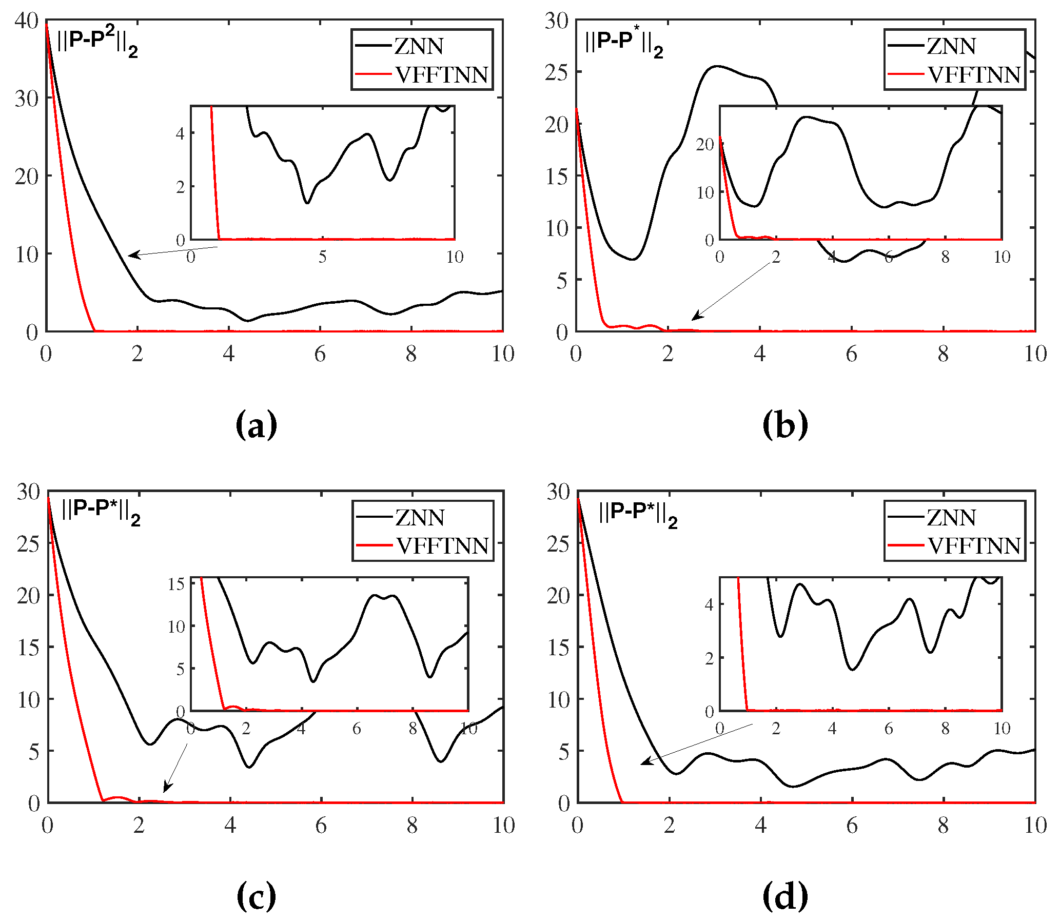
In this section, we will verify the robustness of VFFTNN and compare it with ZNN. In order not to lose generality and simplicity, the differentiation and model-implementation errors are considered. For simulation purposes, let us set the differentiation and model-implementation errors as follows
where , and are the settable factors, which can adjust the size of these disturbances.
Here, we will take the four cases in Figure 6 as examples to compare the robustness of VFFTNN and ZNN. Form Figure 6, it can be seen that when , even though the disturbances are small, but the computation error of ZNN cannot converge to 0. On the contrary, when we look at the curve of VFFTNN, we can see that the computation error has converged around 4 seconds. Then look at the other three cases, the computation error of VFFTNN converges to zero, although the disturbances are much larger. Deserving to be mentioned, the convergence time of VFFTNN will be smaller with the design factors increases or decreases.
In conclusion, although the convergence performance of VFFTNN will get worse in the presence of disturbance, it can still complete the convergence and no matter how big the disturbance is, it can converge to 0 in a finite time, which well confirms the robustness of VFFTNN.
5. Conclusions
In this paper, we propose a new neural network called VFFTNN, and discuss the finite-time convergence and robustness of the network for solving Sylvester equation under three different activation functions. Compared with the typical ZNN, the proposed VFFTNN increases the time-varying coefficient and the fractional power term, which accelerates the convergence speed of VFFTNN and enhances the anti-jamming ability. More importantly, VFFTNN can guarantee not only finite time convergence, but also super-exponential convergence rate. Simulation results show the superior performance of the neural network for solving Sylvester equation problem. Therefore, in the real hardware implementation, the new neural network has more advantages.
References
- Wei Q, Dobigeon N, Tourneret J Y, et al. R-FUSE: Robust fast fusion of multiband images based on solving a Sylvester equation[J]. IEEE signal processing letters, 2016, 23(11): 1632-1636.
- Wang L, Li D, He T, et al. Manifold regularized multi-view subspace clustering for image representation[C]//2016 23rd International Conference on Pattern Recognition (ICPR). IEEE, 2016: 283-288.
- Hu H, Lin Z, Feng J, et al. Smooth representation clustering[C]//Proceedings of the IEEE conference on computer vision and pattern recognition. 2014: 3834-3841.
- Jang J S, Lee S Y, Shin S Y. An optimization network for matrix inversion[C]//Neural information processing systems. 1987.
- Fa-Long L, Zheng B. Neural network approach to computing matrix inversion[J]. Applied Mathematics and Computation, 1992, 47(2-3): 109-120.
- Cichocki A, Unbehauen R. Neural networks for solving systems of linear equations and related problems[J]. IEEE Transactions on Circuits and Systems I: Fundamental Theory and Applications, 1992, 39(2): 124-138.
- Xia Y, Wang J. A recurrent neural network for solving linear projection equations[J]. Neural Networks, 2000, 13(3): 337-350.
- Zhang Y, Wang J. Recurrent neural networks for nonlinear output regulation[J]. Automatica, 2001, 37(8): 1161-1173.
- Li S, Li Y. Nonlinearly activated neural network for solving time-varying complex Sylvester equation[J]. IEEE transactions on cybernetics, 2013, 44(8): 1397-1407.
- Xiao L, Liao B, Luo J, et al. A convergence-enhanced gradient neural network for solving Sylvester equation[C]//2017 36th Chinese Control Conference (CCC). IEEE, 2017: 3910-3913.
- Zhang Z, Zheng L, Weng J, et al. A new varying-parameter recurrent neural-network for online solution of time-varying Sylvester equation[J]. IEEE transactions on cybernetics, 2018, 48(11): 3135-3148.
- Zhang Y, Jiang D, Wang J. A recurrent neural network for solving Sylvester equation with time-varying coefficients[J]. IEEE Transactions on Neural Networks, 2002, 13(5): 1053-1063.
- Yan X, Liu M, Jin L, et al. New zeroing neural network models for solving nonstationary Sylvester equation with verifications on mobile manipulators[J]. IEEE Transactions on Industrial Informatics, 2019, 15(9): 5011-5022.
- Zhang Z, Zheng L. A complex varying-parameter convergent-differential neural-network for solving online time-varying complex Sylvester equation[J]. IEEE transactions on cybernetics, 2018, 49(10): 3627-3639.
- Deng J, Li C, Chen R, et al. A Novel Variable-Parameter Variable-Activation-Function Finite-Time Neural Network for Solving Joint-Angle Drift Issues of Redundant-Robot Manipulators[J]. IEEE/ASME Transactions on Mechatronics, 2024.
- Xu X, Sun J, Endo S, et al. Variational algorithms for linear algebra[J]. Science Bulletin, 2021, 66(21): 2181-2188.
- Y. Zhang, D. Jiang, and J. Wang, “A recurrent neural network for solving sylvester equation with time-varying coefficients,” IEEE Transactions on Neural Networks, vol. 13, no. 5, pp. 1053–1063, 2002. [CrossRef]
- Li Y, Chen W, Yang L. Multistage linear gauss pseudospectral method for piecewise continuous nonlinear optimal control problems[J]. IEEE Transactions on Aerospace and Electronic Systems, 2021, 57(4): 2298-2310.
- Wang X, Liu J, Qiu T, et al. A real-time collision prediction mechanism with deep learning for intelligent transportation system[J]. IEEE transactions on vehicular technology, 2020, 69(9): 9497-9508.
- Z. Zhang, S. Li, and X. Zhang, “Simulink comparison of varying-parameter convergent-differential neural-network and gradient neural network for solving online linear time-varying equations,” in 2016 12th World Congress on Intelligent Control and Automation (WCICA), 2016, pp. 887–894.
- Y. Zhang, D. Chen, D. Guo, B. Liao, and Y. Wang, “On exponential convergence of nonlinear gradient dynamics system with application to square root finding,” Nonlinear Dynamics, vol. 79, no. 2, pp. 983–1003, 2015. [CrossRef]
- S. Wang, S. Dai, and K. Wang, “Gradient-based neural network for online solution of lyapunov matrix equation with li activation function,” in 4th International Conference on Information Technology and Management Innovation. Atlantis Press, 2015, pp. 955–959.
- W. Ma, Y. Zhang, and J. Wang, “Matlab simulink modeling and simulation of zhang neural networks for online time-varying sylvester equation solving,” Computational Mathematics and Mathematical Physics, vol. 47, no. 3, pp. 285–289, 2008.
- S. Li, S. Chen, and B. Liu, “Accelerating a recurrent neural network to finite-time convergence for solving time-varying sylvester equation by using a sign-bi-power activation function,” Neural Processing Letters, vol. 37, no. 2, pp. 189–205, 2013. [CrossRef]
- Y. Shen, P. Miao, Y. Huang, and Y. Shen, “Finite-time stability and its application for solving time-varying sylvester equation by recurrent neural network,” Neural Processing Letters, vol. 42, no. 3, pp. 763–784, 2015.
- L. Jin, Y. Zhang, S. Li, and Y. Zhang, “Modified znn for time-varying quadratic programming with inherent tolerance to noises and its application to kinematic redundancy resolution of robot manipulators,” IEEE Transactions on Industrial Electronics, 2016.
- M. Mao, J. Li, L. Jin, S. Li, and Y. Zhang, “Enhanced discrete-time zhang neural network for time-variant matrix inversion in the presence of bias noises,” Neurocomputing, vol. 207, pp. 220–230, 2016. [CrossRef]
- L. Xiao and B. Liao, “A convergence-accelerated zhang neural network and its solution application to lyapunov equation.” Neurocomputing, vol. 193, no. Jun.12, pp. 213–218, 2016. [CrossRef]
- B. Liao, Y. Zhang, and L. Jin, “Taylor discretization of znn models for dynamic equality-constrained quadratic programming with application to manipulators,” Neural Networks and Learning Systems IEEE Transactions on, vol. 27, no. 2, pp. 225–237, 2016. [CrossRef]
- Xiao and Lin, “A finite-time convergent zhang neural network and its application to real-time matrix square root finding,” Neural Computing and Applications, 2017.
- Y. Zhang, B. Mu, and H. Zheng, “Link between and comparison and combination of zhang neural network and quasi-newton bfgs method for time-varying quadratic minimization,” IEEE Transactions on Cybernetics, vol. 43, no. 2, pp. 490–503, 2013. [CrossRef]
- Yan D, Li C, Wu J, et al. A novel error-based adaptive feedback zeroing neural network for solving time-varying quadratic programming problems[J]. Mathematics, 2024, 12(13): 2090.
- Zhang, Z.; Lu, Y.; Zheng, L.; Li, S.; Yu, Z.; Li, Y. A new varying-parameter convergent-differential neural-network for solvingtime-varying convex QP problem constrained by linear-equality. IEEE Trans. Autom. Control 2018, 63, 4110–4125.
- R. A. Horn and C. R. Johnson, “Topics in matrix analysis, 1991,” Cambridge University Presss, Cambridge, vol. 37, p. 39, 1991.
- G. Strang and L. Freund, “Introduction to applied mathematics,” Journal of Applied Mechanics, vol. 53, no. 2, p. 480, 1986. [CrossRef]
- C. Mead and M. Ismail, Analog VLSI implementation of neural systems. Springer Science & Business Media, 2012, vol. 80.
- Y. Zhang, G. Ruan, K. Li, and Y. Yang, “Robustness analysis of the zhang neural network for online time-varying quadratic optimization,” Journal of Physics A: Mathematical and Theoretical, vol. 43, no. 24, p. 245202, 2010. [CrossRef]
Figure 1.
Block diagram of VFFTNN model in order to solve Sylvester equation.
Figure 2.
Solving Sylvester equation (1) with given coefficients online with ZNN and its computational error . (a)Solution to ZNN with and error of ZNN with . (b)Solution to ZNN with and error of ZNN with . (c)Solution to ZNN with and error of ZNN with .
Figure 2.
Solving Sylvester equation (1) with given coefficients online with ZNN and its computational error . (a)Solution to ZNN with and error of ZNN with . (b)Solution to ZNN with and error of ZNN with . (c)Solution to ZNN with and error of ZNN with .
Figure 3.
Solving Sylvester equation (1) with given coefficients online with VFFTNN and its computational error (). (a)Solution to VFFTNN with and error of VFFTNN with . (b)Solution to VFFTNN with and error of VFFTNN with . (c)Solution to VFFTNN with and error of VFFTNN with .
Figure 3.
Solving Sylvester equation (1) with given coefficients online with VFFTNN and its computational error (). (a)Solution to VFFTNN with and error of VFFTNN with . (b)Solution to VFFTNN with and error of VFFTNN with . (c)Solution to VFFTNN with and error of VFFTNN with .
Figure 4.
When ZNN uses different activation functions without perturbation to solve Sylvester equation (1), its convergence error is as shown above(). (a)Linear. (b)Sigmoid. (c)Power().
Figure 4.
When ZNN uses different activation functions without perturbation to solve Sylvester equation (1), its convergence error is as shown above(). (a)Linear. (b)Sigmoid. (c)Power().
Figure 5.
When VFFTNN uses different activation functions without perturbation to solve Sylvester equation (1), its convergence error is as shown above( and ). (a)Linear. (b)Sigmoid. (c)Power().
Figure 5.
When VFFTNN uses different activation functions without perturbation to solve Sylvester equation (1), its convergence error is as shown above( and ). (a)Linear. (b)Sigmoid. (c)Power().
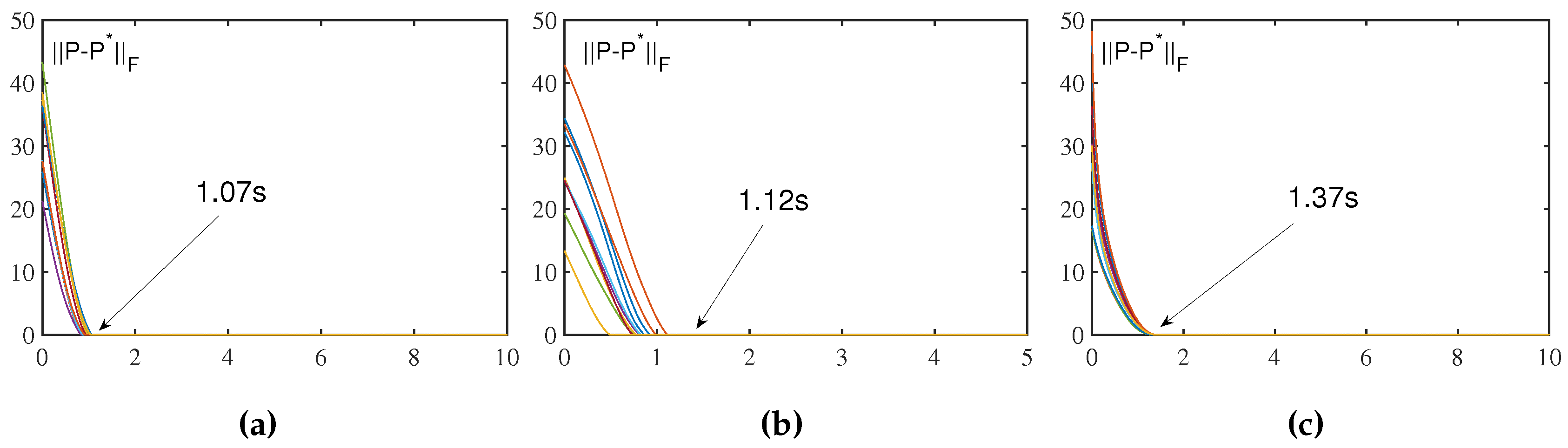
Figure 6.
Robustness of ZNN and VFFTNN with varying degrees of differential error and model implementation error. (a). (b) and . (c) and . (d) and .
Figure 6.
Robustness of ZNN and VFFTNN with varying degrees of differential error and model implementation error. (a). (b) and . (c) and . (d) and .
Disclaimer/Publisher’s Note: The statements, opinions and data contained in all publications are solely those of the individual author(s) and contributor(s) and not of MDPI and/or the editor(s). MDPI and/or the editor(s) disclaim responsibility for any injury to people or property resulting from any ideas, methods, instructions or products referred to in the content. |
© 2024 by the authors. Licensee MDPI, Basel, Switzerland. This article is an open access article distributed under the terms and conditions of the Creative Commons Attribution (CC BY) license (http://creativecommons.org/licenses/by/4.0/).
Copyright: This open access article is published under a Creative Commons CC BY 4.0 license, which permit the free download, distribution, and reuse, provided that the author and preprint are cited in any reuse.


