
Submitted:
14 November 2024
Posted:
15 November 2024
You are already at the latest version
Abstract
The combination of highly dynamic systems with a limited work envelope, with a less dynamic system with a larger working envelope, promises to combine the advantages of both systems while eliminating the disadvantages. For these systems separation algorithms determine the trajectories based on the target geometries. However, arbitrary processing orders of these result in inefficient trajectories because successive geometries maybe geometrically far apart. This causes the dynamic system to operate below its potential. Current planning tools do not optimise the processing order for such redundant systems. The aim is to design and implement a planning tool, for the application of laser marking. The tool considers the processing order of the 2D geometries from a geometric point of view. The resulting sequenced path data can then be used by trajectory generation algorithms to make full use of the potential of redundant systems. The approach analyses literature on Travelling Salesman Problems (TSP), which is then transferred to the given application. A heuristic and a genetic algorithm are developed and integrated into a planning tool. The results show the heuristic algorithm being faster, while still producing solutions whose total path length is similar to that of the genetic algorithm. Even though, the solutions don’t meet any optimality standards, the presented automated approaches are superior to manual approaches and are to be seen as a starting point for further research.
Keywords:
CAM
; galvanometer scanner
; laser applications
; path planing
; redundant axes
1. Introduction
Businesses are required to be economically competitive. In a manufacturing context, this can be achieved my making production processes more productive and or capable. One approach to this is, the combination of a highly dynamic system with a limited work envelope, with a less dynamic system with a larger working envelope. This promises to combine the high productivity associated with highly dynamic systems with a large working envelope of the larger system. This can then for example reduce job set-up times by sequentially processing many small jobs in one big job. Furthermore, the enhanced work envelope also extends the range of applications the production process can be used for. In laser applications such as additive manufacturing, polishing, cutting, welding and marking the dynamic system component is often represented by a galvanometer scanner [1,2,3]. It can be used to position a laser spot in a xy-plane. However, the maximum work envelope, i.e. the maximum scan field is restricted by the following aspects: One, the maximum mechanical angular deflection of the mirrors in a given scanner, and the distance between the mirrors and the target Pelsue.1983. Two, the focal length of the commonly used F-Theta lenses, which are employed to focus the laser onto the scan field. The focal length is proportional to the laser spot diameter [1][p. 37]. Increasing the focal length extends the work envelope, but it also increases the laser sport diameter. As the laser spot diameter has a manufacturing process dependent upper limit, increasing the work envelope by adjusting the focal length is also limited. To further increase the work envelope, the scanner is mounted on a larger secondary kinematic system, referred to here as the base system. It moves the scanner to increase the overall work envelope. An example of this could be a xy-system, as illustrated in Figure 1).
There are two primary methods of combining the scanner and base system operation: sequential and simultaneous. In the sequential method, known as step-and-scan, the scanner processes parts within its scan field before the base system moves the scanner to the next field [4,5]. In the simultaneous method, known as on-the-fly-scanning, both systems move together. Using the on-the-fly-scanning method allows for higher overall productivity at the expense of complexity in trajectory planing [4,5,6,7,8]. The complexity stems from the fact that there are infinite ways to separate the tool center point (TCP) path between the two systems. In this work, the TCP path describes the position of the scanners laser spot in the combined work envelope of both systems (see eq:tcpxy). Besides separating the original path into two, the trajectory generation methods must also consider the different dynamic capabilities of the systems.
Effective on-the-fly-scanning and the linked trajectory generation methods require a strategic processing sequence to make full use of the dynamic potential of a redundant system. An example for a strategic and non-strategic sequence is given in Figure 2). In (a) the processing order is arbitrary. Because of this, the base system has to move the scanner along a longer than necessary path to cover all geometries. In (b) the rectangles are processed in a strategic manner, allowing the scanner to be swept from left to right while processing all target geometries.
WWhen using redundant kinematic scanner systems with different work envelopes and dynamics, it is crucial to plan the TCP path to strategically utilise both systems. Otherwise, long traversal paths of the base system require the scanner system to act far below its dynamic limits, or stay idle until the next processing area is reached. This planing is executed in computer aided manufacturing (CAM) tools. This paper specifically focuses on CAM solutions for redundant systems with different work envelopes and dynamics, while examining open and closed 2D contours as input geometries for a laser engraving application. In this context, CAM tools can be divided into three types: One, vector graphics tools such as Inkscape, Adobe Illustrator or Affinity Designer with plug-ins for gcode export. Two, CAM tools such as Lightburn, LaserGRBL or Snapmaker Luban for laser cutting and engraving. And three, specialist tools, such as Aerotech’s CADFusion, or Direct Machining Control which specifically address redundant kinematics. The first two categories do not address the unique requirements of redundant systems and require manual intervention to define a strategic processing order, which is impractical for production environments. The third type, specialist tools, are either tailored to specific manufacturers’ hardware and or it is not evident how the underlying algorithms work. To the authors’ knowledge, no research specifically addresses the problem of strategic path planning for redundant systems with different work areas and system dynamics. While examples such as [9] and [10] examine similar issues, these findings are not directly transferable to the here described application. Furthermore, the existing literature on path planing is also not directly applicable to CAM tools, as the underlying traveling salesman problem (TSP) needs to be abstracted and supplemented with additional constraints. Why this is the case will be explained in sec:CAM Concept Overview. Given the limitations in the state of research regarding laser CAM tools for redundant systems with different work envelopes and dynamics, the objectives of this paper are:
- (1)
- To adapt the problem of strategic path planning for redundant systems with different work envelopes and dynamics to the path planning problems discussed in the existing literature.
- (2)
- To conceptualise and implement a tool designed for this specific purpose.
- (3)
- To discuss the performance of the developed tool based on test cases.
This paper assumes that the CAM and path separation & trajectory planning algorithm are separate from each other, and that the latter is responsible for the dynamics planning. Consequently, the CAM tool developed in this paper will focus on finding geometric solutions and will not consider dynamics of a given system. This is further discussed in subsec: General discussion. This paper is structured as follows: Section 2 will present the concept of the CAM tool and introduce the fundamentals of a clustered global traveling salesman problem (CGTSP) and a genetic algorithm (GA), which will be extended and applied to the CAM tool in sec:Implementation. Section 5 will highlight the results generated by the developed CAM tool. Finally, sec: Conclusion will summarise the findings and give an outlook on where further research is needed.
2. Materials and Methods
This section will present the concept for the CAM tool and introduce fundamentals on the topics of CGTSP and GA.
2.1. CAM Concept Overview
In a first step, input data is processed. As stated above, the CAM tool presented in this paper focuses on open and closed 2D geometries. Thus, input data is chosen to be in the form of scalable vector graphics (SVG) files. The individual geometries contained in SVG files, such as paths, ellipses, rectangles and circles are discretised into groups of individual vertices. In the second step, the scan field optimization takes place. This step determines the number and location of required scan fields to cover all geometries, which have to be processed (see Figure 3). The third step is to run one of the two strategic path planning algorithms presented. These decide one, the order in which the individual scan fields are processed. Second, the order in which the geometries within each scan field are processed. And third, the start and end vertices of each geometry. The final and fourth step is to export the generated data as gcode. The gcode contains all the TCP path data in a strategic order. This data can then be used as input for algorithms responsible for separating the TCP path and trajectory planing. However, these are not considered in this paper. The overlaying problem of steps two and three is finding an optimal path that connects all the geometries, more specifically the vertices into which the geometries are discretised. This path should be as short as possible. For the concrete application, this means that the sum of idle paths, those that are inserted in-between geometries, where the laser is turned off, is as short as possible. Furthermore, it is desired that the path which describes the motion of the scan fields across the entire work envelope is also as short as possible, i.e. that the base system moves the scanner as little as possible. In consequence, the dynamically, much more capable scanner is made responsible for executing a large part of the motion, during the trajectory planing phase.
2.2. TSP Classification and Solution
The problem of finding the shortest, path that connects individual vertices can be classified as a TSP. The classic TSP involves finding the shortest possible path that visits each city, i.e. vertex, once and returns to the origin vertex, given a list of vertices and the cost to travel between each vertex. This problem is NP-hard [11], meaning there is no known algorithm that can find the optimal solution in polynomial time. For a problem with n vertices, the computational complexity is and grows exponentially with the number of vertices. Depending on the application and associated constraints, a TSP can be further classified as a clustered traveling salesman problem (CTSP) [12,13,14,15], global traveling salesman problem (GTSP) [16,17,18,19,20,21], CGTSP [9,10,22,23] and family traveling salesman problem (FTSP) [24]. For the described use case of a CAM tool, the classification as a CGTSP is appropriate. Why this is the case will be explained in CGTSP. Different approaches exist to solve these problems, some of them are: exact algorithms, such as the branch and bound [25] and cutting plane method [26]. These find optimal solutions by exploring all possible paths. However, they are only practical for small to medium-sized problems due to exponential computation time [11]. Heuristic algorithms, including Nearest Neighbour [27], Greedy, 2-opt [28], Lin-Kernighan-Helsgaun [20], Simulated Annealing [29], GA [19,30] and Ant Colony Optimisation [21], provide faster solutions. These heuristics use strategies such as local search improvement and probability-based selection, making them suitable for a variety of problem sizes. While exact algorithms guarantee optimal solutions, heuristics balance solution quality and computation time, making them ideal for larger problems. Consequently, this paper will look at two heuristic approaches. Why this is done will be further dicusssed in subsec: General discussion.
2.3. Clustered Global Travelling Salesman Problem
Before introducing solutions for solving a CGTSP, it itself will be introduced and put in the context of a CAM tool. In a CGTSP the goal is to find the shortest path that: visits each cluster, i.e. scan field where each scan field must be visited exactly once. In each scan field, there are several sub-cluster (SC), i.e. geometries. From these geometries, exactly one vertex of the geometry, has to be visited. The CGTSP can be understood through a graph , where V represents a set of vertices, and E represents a set of edges. The vertex set V is divided into k non-empty subsets, denoted as , , ..., , which are referred to as clusters. Therefore, it meets the following conditions [10]:
Additionally, each cluster’s vertices are further divided into several SC. In the graph, there are two types of edges: those connecting vertices of SC within the same cluster, and those connecting vertices of SC across different clusters. The cost function c is associated with each edge , expressed as , referred to as the edge cost. The CGTSP seeks the least costly path H that satisfies the following properties [10]:
- H visits precisely one vertex from each SC
- All SC belonging to the current cluster are visited consecutively before moving to the next cluster.
Figure 3 illustrates the CGTSP applied in the context of a CAM tool, along with two feasible solutions, which are separately shown with yellow and green lines. The order of geometries for the yellow solution is: 1-0-6-4-5-3-2, and the order of geometries for the green solution is: 0-1-2-3-5-4-6. The instance shown in this figure includes 135 vertices, divided into three clusters, i.e. scan fields, , , . These are indicated as blue fields. Furthermore, each cluster’s vertices are divided into multiple SC, i.e. geometries, , , and .
The CGTSP in this application differs from the general CGTSP in several ways:
- SC, i.e. geometries, need to be treated as two variants: one, closed geometries, such as , , , where all vertices within a SC are visited sequentially, and only one vertex needs to be selected as the start and end point. The other variant is an open geometry, such as , where one of two end vertices must be chosen as the start point of the open geometry’s scanning trajectory, with the other serving as the end point. This is the case as stitching together a continuous segment out of several segments is usually visible and an undesirable process result.
- There is no need to complete a circuit, i.e. there is no need to return to the starting geometry once arrived at the final geometry. Thus, the distance from the last to the first geometry vertex is not considered within the route.
- Within each cluster, the visiting order of the SC should be as directional as possible, starting from the SC closest to the previous cluster and moving towards the next cluster. Consequently, the number of direction changes should be kept low. The idea being, that if there is an overlying processing direction, e.g. from left to right, then the motion of the scanner and the base system will also follow this overlying direction. This then serves as the basis for the path separation algorithms to find a feasible solution which makes uses of the combined system dynamics while adhering to the stroke limitations of both systems (see Figure 2).
2.4. Genetic Algorithm
Genetic Algorithms are a class of search algorithms that are fundamentally rooted in the principles of natural selection and genetics [30]. To address the CGTSP, a chromosome needs to be structured to encapsulate information pertinent to the solution it represents.
2.4.0.1. Encoding of a Chromosome
The chromosome data structure consists of two primary components: The sub-cluster order (SCO) and the vertex order (VO). The SCO defines the order in which SC, i.e. geometries, are processed. The VO determines the start-end vertex of a SC. Each element in the SCO and the VO correspond to each other. Following the SCO and VO provides a feasible solution to the CGTSP [10].
An example for two chromosomes is given in eq:chr1 and eq:chr2. These represent possible solutions to the CGTSP depicted in Figure 3. eq:chr1 is represented by the yellow path and eq:chr2 by the green path.
Generally, GAs start by constructing various chromosomes to form an initial population, ensuring diversity within the population. Through a survival-of-the-fittest selection method, individuals with higher fitness undergo crossover and mutation to produce superior offspring, and this process is repeated across multiple generations. In the case of the CAM tool, the fitness may for example represent the total path length required to process all geometries. Crossover involves inheriting genes from parent chromosomes to form new offspring, which are then subject to random mutations at a certain probability to prevent the population from converging on local optima. This mechanism ensures that, over generations, increasingly optimal solutions are generated until a termination criterion is met [30]. Details about the initial population, selection methods, crossover, mutation, and termination criteria will be discussed in Section 3.3.
3. Implementation
The implementation section will first highlight the scan field optimization, which finds the required number and location of scan fields to cover all geometries. After this, the two path optimisation algorithms are presented which determine the path connecting the SC, i.e. geometries in and across the scan fields.
3.1. Scan Field Optimisation
After importing the geometric data, it is crucial to cover all geometries with as few scan fields as possible. This process is depicted in Figure 4 where scan fields, blue squares, are distributed over the "ISW" shaped geometries. By minimizing the number of scan fields, each geometry can ideally be allocated to only one scan field. If this isn’t the case, further steps need to be taken to assign each geometry to a scan field. Furthermore, by minimising the number of scan fields, the TSP linked to finding a path that connects these is simplified (see subsec:Path Planning Method for Scanfields). As galvanometer scanners suffer from distortion, which increases at the edges of the scan field, it is desirable to set the cluster position as centred as possible among the geometries. Consequently, the scan field optimisation also considers this. The steps to optimize the position of clusters are depicted in Figure 4 and described in the following:
- (1)
- Initial generation: Randomly generate a certain number of scan fields (e.g., 256) within the combined work envelope of the scanner and base system.
- (2)
- Coverage check: Check whether all geometries are covered. If not, repeat step 1.
- (3)
- Scan field reduction test: Try to remove each scan field individually and check if all geometries can still be fully covered. If so, remove that scan field; if not, retain it. This step preliminarily reduces the number of scan fields.
- (4)
- First optimization of scan field positions: Move each scan field, individually, to reduce the total area covered by all scan fields while still ensuring all geometries are covered. Next repeat step three, to further reduce the number of scan fields. During the moving of scan fields, each is displaced by a defined unit of length in the positive and negative spatial directions and diagonals. After each displacement, a check is made to see whether an improvement has occurred.
- (5)
- Second optimization of scan field positions: Move each scan field as in step four, to try to reduce the overlapping areas of scan field while ensuring all geometries are still covered, and then repeat step three. This again tries to minimize the number of scan fields.
- (6)
- Third optimization of scan field positions: Move each scan field to position all geometries as centrally as possible within the scan field, enhancing scanning quality.
Once the optimized scan field positions are determined, all geometries are allocated to their respective scan fields in an unordered manner. It is important to note that some geometries may be covered by multiple scan fields. This is, for example, the case for the geometries located in the union of the bottom left two scan fields, highlighted by the gray dashed box, in Figure 4 e). In such cases, it is necessary to compare the shortest distances between these geometries and the other geometries that are already assigned to those multiple scan fields. These geometries should then be separately allocated to the scan field that contains the geometry closest to them. This approach enables the allocation of geometries that are proximate in distance to each other in the same scan field.
3.2. Hierarchical Heuristic Algorithm
For the given problem, a so called hierarchical heuristic algoritm (HHA) is developed that transforms the CGTSP into multiple layers of a TSP. The first, outer, layer is determining the sequence in which scan fields are processed. Then, a heuristic algorithm is employed to select appropriate geometries within each scan field to serve as the starting or terminating element. This selection guides the direction of path planning within the scan field. The inner layer of the TSP is to determine the scanning sequence within each scan field. Subsequently, within each SC, the start and end vertices of the geometries have to be chosen. The vertex enhancement algorithm (VEA) is then utilized to enhance the selection of vertices in each SC. Ultimately, this process effectively yields an optimized TCP path.
3.2.1. Path Planning Method for Scan Fields
The vehicle routing solver in OR-Tools [31] is used to determine the shortest path connecting the centres of all scan fields. The first scan field is selected to be the one closest to the top left corner of the work envelope. To address the non-standard requirement of having distinct start and end points, a virtual endpoint is introduced. The distance from the virtual point to all scan field centres is set to zero, ensuring that any scan field could potentially be the terminating one. Since the number of scan fields is generally low, compared to the number of geometries contained within it, the path cheapest arc (PCA) in the OR-Tools suite, quickly yields a satisfactory solution (see table:TSPPCA).
3.2.2. Path Planning Method within Each Scan field
Using the OR-Tools TSP solver for computation, it is initially necessary to select appropriate geometries, i.e. SC within each scan field to serve as the starting and terminating SCs. Using the function nearest_vertices() imported from the python Shapely library, the starting SC for each scan field is determined by finding the SC in the current scan field that is closest to all SCs in the previous scan field, and similarly, the ending SC by finding the SC that is closest to all SCs in the next scan field. Specifically, for the first scan field, the starting SC is chosen as the one farthest from the intersection of the line connecting the centroids of the first scan field and the second scan field with the boundary of the first scan field. These connecting lines are represented by the green dotted lines in Figure 5. For the last scan field, the ending SC is the one farthest from the intersection of the line connecting the centroids of the last scan field and the second to last scan field with the boundary of the second to last scan field. For cases with only one scan field, the starting SC is the one nearest to the top-left corner of the scan field, and the ending SC is nearest to the bottom-right corner.
Then, the geometries, i.e. SCs, are ordered in each scan field, using OR-Tools, based on their centroid vertex and the previously chosen start and end vertices of each scan field. Additionally, it is ensured that the sequence of geometries has a certain directionality. This is achieved by first choosing geometries that are further away from the end geometry of the respective scan field. Practically, this is implemented by adjusting the distance cost matrix, used in OR-Tools. An extra penalty is added to the distance between the centre of the current geometry and other geometries within the scan field. This penalty is inversely correlated to the distance of other geometries to the next scan field. This is depicted in Figure 5, the penalty imposed on the distance from Geometry 0 to Geometry 1 is inversely correlated with the length of the segment AB (see eq:costwithpenalty).
Point B represents the intersection of the line connecting the centroids of and with the boundary of , whereas point A denotes the projection of the centroid of Geometry 1 onto this line. Particularly, for the last scan field, the added penalty is positively related to the distance to the previous scan field; for the cases with only one scan field, the added cost is inversely related to the distance to the last SC in the scan field. The adjusted cost D is mathematically expressed in eq:scanfieldopticost where the subscripts c and n represent the current vertex and the possible next vertex. represents the slope of the line connecting the centroids of the current scan field j and the next scan field, the subscript i represents the intersection of the aforementioned line with the boundary of the current scan field, and is the diagonal length of the scan field.
Through testing, it has been determined that using the PCA, from OR-Tools, as an initial solution, along with the penalized distance cost matrix, provides favourable direction-oriented solutions. When using the guided local search (GLS) strategy, from OR-Tools, to attempt escaping local optima, the solutions often show poor directionality (see Figure 6). Therefore, this strategy is not used in cases with multiple scan fields. However, for cases with only one scan field, where the directional demands for path scanning are comparatively low, the penalty weight of in Equation 4a substituted with a smaller weight of and the GLS is chosen. Under a time limit of 30 s, this approach attempts escaping local optima, aiming to improve the initial solution.
Since the starting and ending SCs within each scan field have already been determined, the ordering of SCs within each scan field is independent of each other. To enhance computational efficiency and reduce computation time, parallel processing is used to determine the processing order in each scan field.
3.2.3. Vertex Selection Method within Each Scan field
Once the geometry, i.e. SC, sequence is established, the nearest_vertices() function from the python Shapely package is used to find the vertex in each SC closest to the next SC. This determines an initial set of start-end vertices for each geometry. As this function has no context for the fact that an overall shortest path is trying to be found, its results can be further improved. For example, two geometries with parallel lines can have several vertices which represent a shortest path linking the two. But when considering a subsequent, third geometry, picking a start-end vertices set for the first two which is close to the third is desirable. Thus, the initial start-end vertices chosen need to be improved via the VEA.
After the initial vertex set is determined, the VEA is used to further enhance the selection of vertices on each SC. The VEA looks at the current start-end vertex of a geometry and the previous and next start-end vertex of geometries in the processing order (see Figure 7). The process of the VEA is detailed in the following:
- (1)
- Using Point() from the python Shapely library, each discretised vertex of the current SC is transformed into a point object.
- (2)
- The Shapely LineString() function is used to transform the chosen start-end vertices of the previous and next SCs into a line segment.
- (3)
- All vertices in the current SC are traversed, and the function distance() is used to calculate the distance between each vertex and the line segment created in step 2. The vertex that is closest to the line segment is updated as the chosen vertex for the current SC, i.e. geometry. For open geometries, merely attempting to swap the starting and ending vertices, comparing whether the empty travel distance is reduced; if so, update the starting vertex accordingly.
- (4)
- Repeat the previous steps for all SCs, continuing looping until no more vertices need to be updated.
3.3. Hybrid Genetic Algorithm
The hybrid genetic algorithm integrates a GA with other optimization techniques such as a TSP solver and a customized VEA to enhance genetic convergence and increase the efficiency of the algorithm. The specific implementation steps are depicted in Figure 8.
3.3.0.1. Initial Population
Starting point of the GA is the creation of an initial population, i.e. N initial chromosomes. Each of these N chromosomes has i SC, where i represents the total number of SCs in a given problem. The SCO determines the order in which these SC are visited. Corresponding to each, SC there are also i vertices which indicate the start-end point of the SCs. These values are initialised randomly while adhering to the minimum and maximum SC and respective vertex index. In addition to the random values, two chromosomes are created that all either carry the minimum, i.e. zero, or maximum index for the VO. This is done to prevent the loss of potentially good genes. Furthermore, all chromosomes are constructed via multiprocessing. This is the case as the chromosome enhancement algorithm (CEA), which is explained in the following, is applied to each chromosome in the creation process and thus a non-negligible computation time is required. An example for two initial chromosomes, for the example in Figure 3, are given in eq:Chrinitrandom and eq:Chrinitspecial.
3.3.0.2. Chromosome Enhancement Algorithm
When chromosomes are create the CEA is applied to them. The purpose of this is to increase the convergence speed. The CEA enhancement process is divided into two main steps: The first step uses OR-Tools as a TSP solver to enhance the SCO. The alteration in the SCO is also reflected in the VO; The second step utilizes the VEA to enhance the selection of vertices in VO, without altering SCO. The VEA used here is the same as the VEA used in the HHA, which is not detailed again here. Below, the strategy to enhance SCO using the OR-Tools’ solver for Vehicle Routing is specifically discussed.
Firstly, the coordinate of the top-left corner of the combined base scanner work envelope is set as the starting node coordinate. A virtual point is designated as the termination node, with the distance cost to this virtual point from other nodes set to zero, meaning any vertex could potentially be the termination vertex.
Secondly, OR-Tools PCA is used to improve on the SCO. For this, a customized distance callback function is needed. It is used in OR-Tools to determine the distance between vertices, i.e. the edge cost, of different SCs. By implementing a custom callback function, it is possible to increase the cost of edges crossing scan fields. The additional penalty is at least equal to the maximum length in the scan field, i.e. the diagonal length of the scan field. Thus, making it is possible to ensure that all geometries within the current scan field are visited before moving to the next scan field. Details of the distance callback function are represented in Algorithm 1. It’s important to note that because the same penalty is applied to all edges crossing scan fields, the order of the scan fields may be adjusted based on the internal arrangement of vertices, rather than strictly adhering to the original order of scan fields.
| Algorithm 1:Calculate Distance Callback for Routing |
Ensure:
Result
|
The chromosomes in eq:Chrinitrandomenhan and eq:Chrinitspecialenhan result from applying the CEA to the chromosomes from eq:Chrinitrandom and eq:Chrinitspecial.
3.3.0.3. Selection
The selection is obtained through the elitist selection method. The purpose of elitist selection is to choose superior genes for reproduction. All chromosomes are ranked according to a fitness function. The fitness function is the reciprocal of the target function, which in this case is the sum of the idle travel distances, i.e. the distance connecting geometries, see for example green line in Figure 6. The shorter the idle travel distance, of the total scanning path represented by an individual is, the higher the fitness value, indicating more superior genes.
3.3.0.4. Crossover
The crossover operator generates two offspring chromosomes, denoted by and , by combining two parent chromosomes. From the index range N(SCO), two numbers are randomly drawn, these represent the start- and end-index of the parts of the SCO and the VO that are interchanged between the parent chromosomes to create the offspring.
For instance: use the chromosome in eq:Chrinitrandomenhan as paternal chromosome and the chromosome in eq:Chrinitspecialenhan as maternal chromosome. Here, N(SCO) is 7. Assume 2 and 4 are drawn as start index and end index (i.e., the 3rd and 5th element in SCO). Then the offspring number one will inherit the SC at the indexes 0 and 1 from parent number two. Next, offspring one will get SCs from index 2 to 4 from parent one. Finally, offspring one, will fill the remaining indexes with the SCs from parent number two. The same is done for the VO as this order is directly linked to the SCO. The other offspring chromosome is generated similarly. This aims to avoid duplication of SCs in the offspring and to inherit the excellent genes of the parents as much as possible.
3.3.0.5. Mutation
After crossover, the offspring chromosomes mutate according to a given probability. The mutation operator generates a modified version of the chromosome through the following process: A cluster is randomly selected, and for each SC within , the corresponding vertex in the VO is replaced with another randomly selected vertex from the same SC.
Taking os1 in Eq. 7a as an example of the offspring to be modified, where , , and . Assume is randomly selected as the cluster to be mutated, then a mutated offspring chromosome may be as follows:
where the vertex numbers of and in have been randomly selected as 2 and 5, respectively. Finally, offspring chromosomes need to undergo further processing by CEA, regardless of whether mutations have occurred.
3.3.0.6. Parameter Adjustment
Through testing, the parameters for the GA have been adjusted to the following configuration: The initial population size is set to be three times of the population size , which is set to 32. For the given system and test cases, increasing the population size did not improve the quality of the results. However, the calculation times increased. Based on the selection strategy, the top 20% of the chromosomes from the current population are directly inherited to the next generation. The remaining 80% of the new generation is produced by performing crossover operations times, using random pairs drawn from the top 20% of the current population’s chromosomes as parents. The probability that a crossover-produced offspring undergoes mutation is 30%. ` If the previous generation fails to improve the solution, the current population size will increase by 50%, but not exceed 48. This number is chosen to limit the computation time. However, if the solution was improved in the previous generation, the population size will decrease by 20%, but not fall below 16. This number is chosen to prevent generating solutions, for the given test cases, which converge in local minima. Moreover, the GA will terminate if there has been no improvement for five consecutive generations, or if calculations continue for three generations at the maximum population size, or if the time, excluding the time taken to generate the initial population, exceeds two hours after completing the operations for the current generation.
4. Results
The capabilities of the three introduced optimisation methods: the scan field optimisation, the HHA and the HGA are tested via twelve test cases. These differ in: One, the number of geometries, here a low (, medium () and high ( number is chosen. Two, the resulting number of scan fields. Three, the type of pattern, random or ordered, that the geometries represent. The random patterns consist mainly of rectangles of different sizes. Only SC82C24 contains more complex geometries. This is the case to demonstrate that these can also be handled by the tool. The ordered patterns are ’O’ and ’ISW’ shapes created by smaller rectangles. The different numbers of geometries are chosen to analyse how the computation times of the algorithms scale. The test cases are also created in such a way, i.e. the geometries are distributed over the entire workspace, that different numbers of scan fields have to be generated. Again, this is done to see how the computation times of the algorithms scale. In the case of HHA and HGA, this is also done to see how the computation times vary when a similar number of geometries are distributed over a few or many scan fields. The purpose of the different pattern types is to analyse how the directionality of the solutions differs.
All test cases are calculated for a base system with a xy stroke of 300 x 300 mm and a scanner with a xy stroke of 70 x 70 mm. This is representative of a real world machine available at the Institute for Control Engineering of Machine Tools and Manufacturing Units (ISW). The calculations are performed on a mobile system, Lenovo E480e, with an Intel Core i7-8550U CPU @ 1.8 GHz, a configured thermal design power of 15 W and 8 GB RAM. It is representative of a low to average mobile computing device and highlights if the developed algorithms are applicable to a wide range of devices.
One exemplary result is given in Figure 9. All other results are not depicted here due to space reasons, but can be taken from [32]. However, tab:randompatterncase, tab:orderedpatterncase and table:scan field optimisation summarise the results in a tabular format allowing for their discussion in the following sec:Discussion.
5. Discussion
The following will first discuss the results of the scan field optimisation, see subsec:Scan field optimisation; then go into a comparison of the HHA and the HGA in subsec:Comparison HHA vs. HGA. This is then followed by a general discussion in subsec: General discussion.
5.1. Scan Field Optimisation
The results for the scan field optimisation are summarised in table:scan field optimisation. Further exemplary results can be taken from [32]. Each of the twelve test cases was processed a total of ten times.The results show that as the average number of scan fields increases, so does the standard deviation of the number of scan fields. However, the results are considered stable enough for the application. The results also show that the computation time depends on both the total number of geometries and the number of scan fields, i.e. clusters. Although no direct correlation could be established, the number of scan fields seems to play a more important role when looking at the given results.
The covered area in table:scan field optimisation is calculated by adding up all areas of the scan fields that are only covered once. The overlap is determined by subtracting the covered area from the maximum area that can be covered by a given scan field number and size. The overlap percentage is then derived by normalising the overlapped area by the maximum area that can be covered by a given scan field number and size. Looking at the area covered, the overlap and its standard deviation, it can be seen that the algorithm can be improved. The in part, high overlap percentages and high standard deviations are due to the movement strategy used to optimise the covered area and centre the scan field within the contained geometries. As the movement is gradual, and the improvement is checked after each movement, only local minima can be found. As a result, the initial placement of the scan field has a major influence on the result. The scan fields are then optimised sequentially. Again, local minima can be found because the overall positions of the scan fields are not taken into account.
5.2. Comparison HHA vs. HGA
The path planning results for the twelve test patterns are summarised in tab:randompatterncase and tab:orderedpatterncase. Depictions for every test and can be taken from [32] and a singular example is given in Figure 9.
For both algorithms, the average computation times increase with the number of SC, i.e. geometries. However, as the number of SCs increases, the HHA scales better than the HGA. The HHA requires only between 4.8% and 0.6% (see eq:differences) of the computation time of the HGA for the same given test case. In the case of SC946C32, the HGA was aborted prematurely because it exceeded the specified maximum time limit of two hours, excluding the initial population generation.
For both algorithms, the number of clusters, i.e. scan fields, is also a determining factor. Comparing the average computation times of SC32C2 and SC122C4 with those of SC82C24, where the number of SCs per cluster is much lower, it is clear that distributing the SCs over fewer clusters is beneficial for the computation times. However, it is not possible to establish a direct relationship between the number of SCs and the number of clusters in relation to the computation time.
Comparing the differences in idle stroke distances, as defined by eq:differences for both algorithms, it is evident that HGA performs better at a lower SC count compared to HHA. However, as the SC count increases, the difference between the two becomes smaller.
Analysis of the changes in standard deviation shown in tab:randompatterncase and tab:orderedpatterncase reveals a trend that the number of clusters influences the stability of the results. In particular, a higher number of clusters, indicating a larger coverage area of geometric patterns, results in larger standard deviations in the idle stroke distances obtained by both algorithms. This variability is due to the fact that in scenarios covering large areas, the locations of the clusters generated by the scan field optimisation process are not consistent. In addition, variations in the cluster distributions have the potential to alter the order of the clusters, thus affecting the final solution provided by the HHA. Similarly, the cluster distributions also affect the allocation of SCs, which in turn can alter the final solution, regardless of which of the two algorithms is used. In terms of stability, in the ’O’ cases, the standard deviation of the idle stroke distances obtained by the HGA remains consistently lower than those obtained by the HHA. Conversely, in the ’ISW’ cases, a different dynamic emerges. For small ’ISW’, the HHA achieves a standard deviation of zero for idle stroke, indicating better stability in solutions compared to the HGA. However, as the scale of the cases within the ’ISW’ category increases, the standard deviation of idle stroke distances derived from HHA progressively converges towards and ultimately exceeds that obtained by the HGA in large ’ISW’. This increase in variability is attributed to the growing number of clusters as case size increases, coupled with the variability in cluster distribution in each computation. Ultimately, this instability in cluster distribution, caused by the scan field optimisation, significantly affects the stability of the solutions produced by HHA.
For cases involving the simpler ’O’ type patterns, both algorithms perform well in terms of the directional quality of the solutions. However, for the more complex ’ISW’ type patterns, the solutions obtained by HHA show superior directional performance, benefiting from the additional penalty values built into the algorithm.
Overall, it can be concluded that for the small scale case, the HGA outperforms the HHA in terms of the resulting idle stroke. However, this advantage diminishes as the number of SCs and clusters increases, regardless of the type of pattern, random or oriented. However, in all test cases the HHA outperforms the HGA in terms of directionality.
5.3. General Discussion
The primary objective of this contribution was to develop a tool that strategically selects the order in which geometries are processed with a kinematically redundant system by employing path planing techniques, in the form of a TSP, from existing literature. Furthermore, the tools’ performance was to be discussed
The developed tool can already do several things well: One, it can import different shapes, e.g. lines, rectangles, paths etc. from SVG files to order them and export them into gcode. Two, the tool can accomplish the ordering process, in the case of the HHA, for many, approximately 1000, geometries in under a minute using a low to average mobile computing device. This is especially impressive when considering the number and scale of the TSP being solved and the fact that optimal solutions to TSPs are NP-hard [11]. Thus, the tool represents a significant improvement over manually selecting the processing order of geometries, as hast to be done with the tools named in sec:Introduction. Three, the tool can strategically define the start and end vertex for every geometry. This is not possible when manually selecting the processing order of geometries, using the tools named in sec:Introduction.
However, there are also aspects that can be improved: One, the chosen optimisation methods may not be optimal for the given problem. They are primarily selected because it was expected that computation times would scale well with the given problem size, see HHA. Even though determining exact optimal solutions is not feasible given the problem size, different heuristic algorithms than those used may be faster. Two, the modifications made to the algorithms are a result of intuitive reasoning. Consequently, better solutions may exist. Three, the entire premise of the developed tool is that the optimisation is geometric in nature. Thus, path lengths are minimised by solving TSPs. However, the underlying problem, of traversing a kinematically redundant system over a set of geometries, is a dynamic problem. Consequently, a solution with an overall longer TCP path may be more optimal in terms of the overall processing time than a solution with a shorter overall TCP path. Ideally, the problem of strategic path planing discussed in this paper is combined with the trajectory plaining for the redundant systems. However, as stated in the introduction in sec:Introduction the two problems are in a first step treated separately to simplify them. Given experience with both sub problems, solutions can then be developed which consider all aspects in one singular optimisation problem.
6. Conclusions
The CAM tool developed in this paper is targeted at the application of laser marking of 2D geometries with a redundant galvanometer scanner based system, where both systems move in parallel during processing. The CAM tool first imports 2D geometries from an SVG file. Then, a scan field optimisation procedure determines the number and positions of scan fields to cover all geometries. Next, either a heuristic or genetic algorithm is used to optimise the order of the geometries based on geometric constraints, i.e. shortest paths. The output is stored as gcode, which can then be used to determine trajectories for both systems.
The results of the test case comparison show that the proposed solution provides a viable solution. However, the variability of the scan field optimisation with each computation still inevitably affects the quality and stability of the solutions derived from both algorithms. Furthermore, both the scan field optimisation and the genetic algorithm suffer from long computation times. The heuristic approach, on the other hand, provides acceptable solutions in a reasonable time frame. Therefore, for further development, it is recommended to improve the scan field optimisation algorithm and the heuristic algorithm, while not pursuing the genetic algorithm.
This work assumes that the process order optimisation, of for example 2D geometries, and the algorithms that then perform the trajectory planning, and thus the trajectory planning, for kinematically redundant systems are separated. This simplifies the problem on the one hand. On the other hand, it also introduces limitations, as a geometrically based process order optimisation does not take the system dynamics into account. Therefore, future research will investigate a holistic approach that can both optimise the process order and perform trajectory planning and path separation.
It should be emphasised that although the CAM tool created is aimed at a specific application, 2D laser marking, the results can be used and extended to other applications and systems. Related laser-based applications that can make use of these results include, but are not limited to: additive processes, cutting, polishing and welding. An example of a less related process would be path planning for photographic drones. Here, the combination of a gimbal-mounted and orientable camera with a drone would also provide a kinematically redundant system. Here, distributed targets need to be flown to by the fastest possible path.
Author Contributions
Conceptualization, D.K., C.R and Y.J.; methodology, D.K., C.R and Y.J.; software, C.R and Y.J.; validation, D.K. and Y.J.; formal analysis, Y.J.; writing—original draft preparation, D.K and Y.J.; writing—review and editing, D.K., C.R and Y.J..; visualization, D.K. and Y.J; supervision, D.K.; project administration, D.K.; funding acquisition, A.V. All authors have read and agreed to the published version of the manuscript.
Funding
This research is funded by the Federal Ministry for Economic Affairs and Climate Action (BMWK) on the basis of a decision by the German Bundestag. It is also funded by the Ministry of Science, Research and Arts of the Federal State of Baden-Württemberg within the InnovationCampus Future Mobility (ICM).
Abbreviations
The following abbreviations are used in this manuscript:
| CAM | Computer Aided Manufacturing |
| CEA | Chromosome Enhancement Algorithm |
| CGTSP | Clustered Global Traveling Salesman Problem |
| CTSP | Clustered Traveling Salesman Problem |
| FTSP | Family Traveling Salesman Problem |
| GA | Genetic Algorithm |
| GLS | Guided Local Search |
| GTSP | Global Traveling Salesman Problem |
| HGA | Hybrid Genetic Algorithm |
| HHA | Hierarchical Heuristic Algorithm |
| ISW | Institute for Control Engineering of Machine Tools and Manufacturing Units |
| LKH | Lin-Kernighan-Helsgaun |
| MDPI | Multidisciplinary Digital Publishing Institute |
| PCA | Path Cheapest Arc |
| SC | Sub-cluster |
| SCO | Sub-cluster Order |
| SVG | Scalable Vector Graphics |
| TCP | Tool Center Point |
| TSP | Traveling Salesman Problem |
| VEA | Vertex Enhancement Algorithm |
| VO | Vertex Order |
References
- Hügel, H.; Graf, T. Materialbearbeitung mit Laser, 5 ed.; Springer Fachmedien Wiesbaden: Abraham-Lincoln-Str. 46, 65189 Wiesbaden, Germany, 2023. [Google Scholar] [CrossRef]
- Kollbach, C.; Wilhelm, H.; Hartl, C. Arten der Oberflächenbearbeitung mit Laser. In Von der Laserbeschriftung bis zum Lasermaterialabtrag; Springer Fachmedien Wiesbaden, 2023; pp. 95–116. [CrossRef]
- Westkämper, E.; Warnecke, H.J. Einführung in die Fertigungstechnik, 8 ed.; Vieweg + Teubner, 2010; p. 302. [CrossRef]
- Zhu, T.; Ji, S.; Zhang, C.; Yin, Y. On-the-fly laser processing method with high efficiency for continuous large-scale trajectories. The International Journal of Advanced Manufacturing Technology 2023, 129, 2361–2370. [Google Scholar] [CrossRef]
- Wang, X.; Mei, X.; Liu, B.; Sun, Z.; Dong, Z. New linkage control methods based on the trajectory distribution of galvanometer and mechanical servo system for large-range high-feedrate laser processing. The International Journal of Advanced Manufacturing Technology 2023, 127, 3397–3411. [Google Scholar] [CrossRef]
- Haas, T.; Warhanek, M.; Dietlicher, M.; Wegener, K. Increased Productivity for Redundant Laser Scanners Using an Optimal Trajectory Separation Method. International Journal of Automation Technology 2016, 10, 941–949. [Google Scholar] [CrossRef]
- Ruting, A.; Blumenthal, L.M.; Trachtler, A. Model predictive feedforward compensation for control of multi axes hybrid kinematics on PLC. IECON 2016 - 42nd Annual Conference of the IEEE Industrial Electronics Society. IEEE, 2016, pp. 583–588. [CrossRef]
- Bock, M. ; Justus Liebig University Giessen. Steuerung von Werkzeugmaschinen mit redundanten Achsen. PhD thesis, Universitätsbibliothek Gießen, 2010. [CrossRef]
- Baniasadi, P.; Foumani, M.; Smith-Miles, K.; Ejov, V. A transformation technique for the clustered generalized traveling salesman problem with applications to logistics. European Journal of Operational Research 2020, 285, 444–457. [Google Scholar] [CrossRef]
- Cosma, O.; Pop, P.C.; Cosma, L. A Hybrid Based Genetic Algorithm for Solving the Clustered Generalized Traveling Salesman Problem. Hybrid Artificial Intelligent Systems; García Bringas, P., Pérez García, H., Martínez de Pisón, F.J., Martínez Álvarez, F., Troncoso Lora, A., Herrero, Á., Calvo Rolle, J.L., Quintián, H., Corchado, E., Eds.; Springer Nature Switzerland: Cham, 2023; pp. 352–362. [Google Scholar]
- Jünger, M.; Reinelt, G.; Rinaldi, G. Chapter 4 The traveling salesman problem. Handbooks in Operations Research and Management Science 1995, 7, 225–330. [Google Scholar] [CrossRef]
- Laporte, G.; Potvin, J.Y.; Quilleret, F. A tabu search heuristic using genetic diversification for the clustered traveling salesman problem. Journal of Heuristics 1997, 2, 187–200. [Google Scholar] [CrossRef]
- Laporte, G.; Palekar, U. Some applications of the clustered travelling salesman problem. Journal of the Operational Research Society 2002, 53, 972–976. [Google Scholar] [CrossRef]
- Ding, C.; Cheng, Y.; He, M. Two-level genetic algorithm for clustered traveling salesman problem with application in large-scale TSPs. Tsinghua Science & Technology 2007, 12, 459–465. [Google Scholar] [CrossRef]
- Mestria, M. New hybrid heuristic algorithm for the clustered traveling salesman problem. Computers & Industrial Engineering 2018, 116, 1–12. [Google Scholar] [CrossRef]
- Noon, C.E.; Bean, J.C. An Efficient Transformation Of The Generalized Traveling Salesman Problem. INFOR: Information Systems and Operational Research 1993, 31, 39–44. [Google Scholar] [CrossRef]
- Laporte, G.; Asef-Vaziri, A.; Sriskandarajah, C. Some Applications of the Generalized Travelling Salesman Problem. Journal of the Operational Research Society 1996, 47, 1461–1467. [Google Scholar] [CrossRef]
- Ben-Arieh, D.; Gutin, G.; Penn, M.; Yeo, A.; Zverovitch, A. Transformations of generalized ATSP into ATSP. Operations Research Letters 2003, 31, 357–365. [Google Scholar] [CrossRef]
- Snyder, L.V.; Daskin, M.S. A random-key genetic algorithm for the generalized traveling salesman problem. European Journal of Operational Research 2006, 174, 38–53. [Google Scholar] [CrossRef]
- Keld Helsgaun. Solving arc routing problems using the Lin-Kernighan-Helsgaun algorithm, 2014.
- Yang, J.; Shi, X.; Marchese, M.; Liang, Y. An ant colony optimization method for generalized TSP problem. 1002-0071 2008, 18, 1417–1422. [Google Scholar] [CrossRef]
- Mohammad Mehdi Sepehri. ; Seyyed Mahdi Hosseini Motlagh.; Joshua Ignatius. https://www.degruyter.com/document/doi/10.1515/IJNSNS.2010.11.9.701/xml. International Journal of Nonlinear Sciences and Numerical Simulation 2010, 11, 701–704. [Google Scholar]
- Foumani, M.; Moeini, A.; Haythorpe, M.; Smith-Miles, K. A cross-entropy method for optimising robotic automated storage and retrieval systems. International Journal of Production Research 2018, 56, 6450–6472. [Google Scholar] [CrossRef]
- Bernardino, R.; Paias, A. Solving the family traveling salesman problem. European Journal of Operational Research 2018, 267, 453–466. [Google Scholar] [CrossRef]
- Egon, B.; Toth, P. Branch and Bound Methods. The Traveling Salesman Problem: A Guided Tour of Combinatorial Optimization.
- Padberg, M.; Rinaldi, G. A Branch-and-Cut Algorithm for the Resolution of Large-Scale Symmetric Traveling Salesman Problems. SIAM Review 1991, 33, 60–100. [Google Scholar] [CrossRef]
- Hurkens, C.A.; Woeginger, G.J. On the nearest neighbor rule for the traveling salesman problem. Operations Research Letters 2004, 32, 1–4. [Google Scholar] [CrossRef]
- Paulo R d O, Costa.; Jason, Rhuggenaath.; Yingqian, Zhang.; Alp Akcay. Learning 2-opt Heuristics for the Traveling Salesman Problem via Deep Reinforcement Learning. <italic>Asian Conference on Machine Learning</italic> <b>2020</b>, pp. Paulo R d O Costa.; Jason Rhuggenaath.; Yingqian Zhang.; Alp Akcay. Learning 2-opt Heuristics for the Traveling Salesman Problem via Deep Reinforcement Learning. Asian Conference on Machine Learning.
- Geng, X.; Chen, Z.; Yang, W.; Shi, D.; Zhao, K. Solving the traveling salesman problem based on an adaptive simulated annealing algorithm with greedy search. Applied Soft Computing 2011, 11, 3680–3689. [Google Scholar] [CrossRef]
- Lambora, A.; Gupta, K.; Chopra, K. Genetic Algorithm- A Literature Review. 2019 International Conference on Machine Learning, Big Data, Cloud and Parallel Computing (COMITCon). IEEE, 2019. [CrossRef]
- Furnon, V.; Perron, L. OR-Tools Routing Library, 07. 05. 2024.
- Kurth, D. Data for, a CAM related, publication in the ZIM IntelliLab project, 2024. [CrossRef]
Figure 1.
Schematic depiction of a redundant system. The axes of the base system are denoted by ’b’ while the axes of the scanner are denoted by a ’s’. The work envelope of the scanner is denoted by the rectangle containing the red laser dots. The combined work envelope of both systems is denoted by the large dotted rectangle.
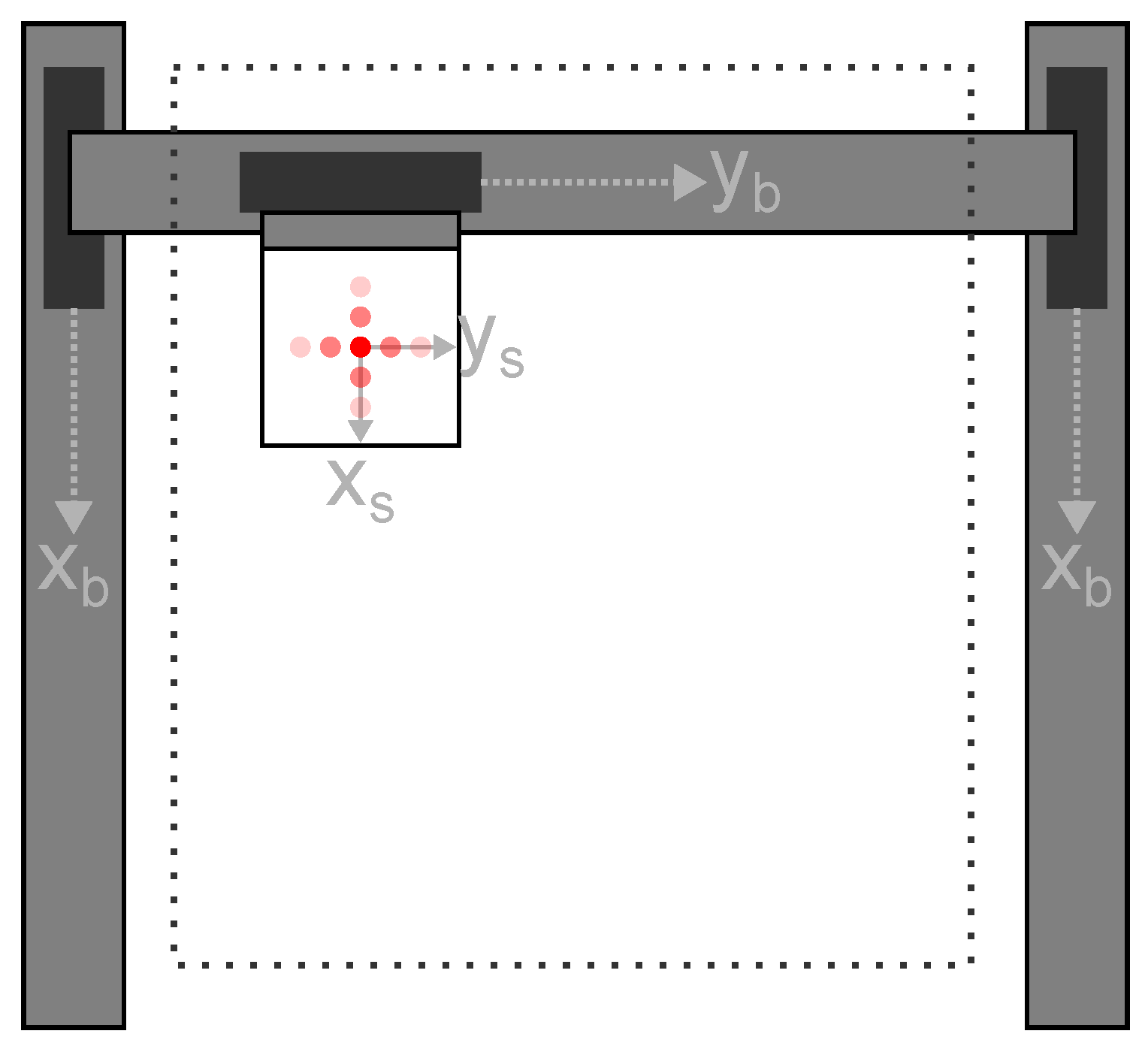
Figure 2.
Exemplary CAM path planing for a 2D brick wall like pattern. The orange rectangles indicate the to be laser marked pattern. The green indicates the processing order of the rectangles. The large blue square indicates the work envelope of the scanner and the blue dotetd line indicates the path of the base system, i.e. the centre position of the scanner while processing.
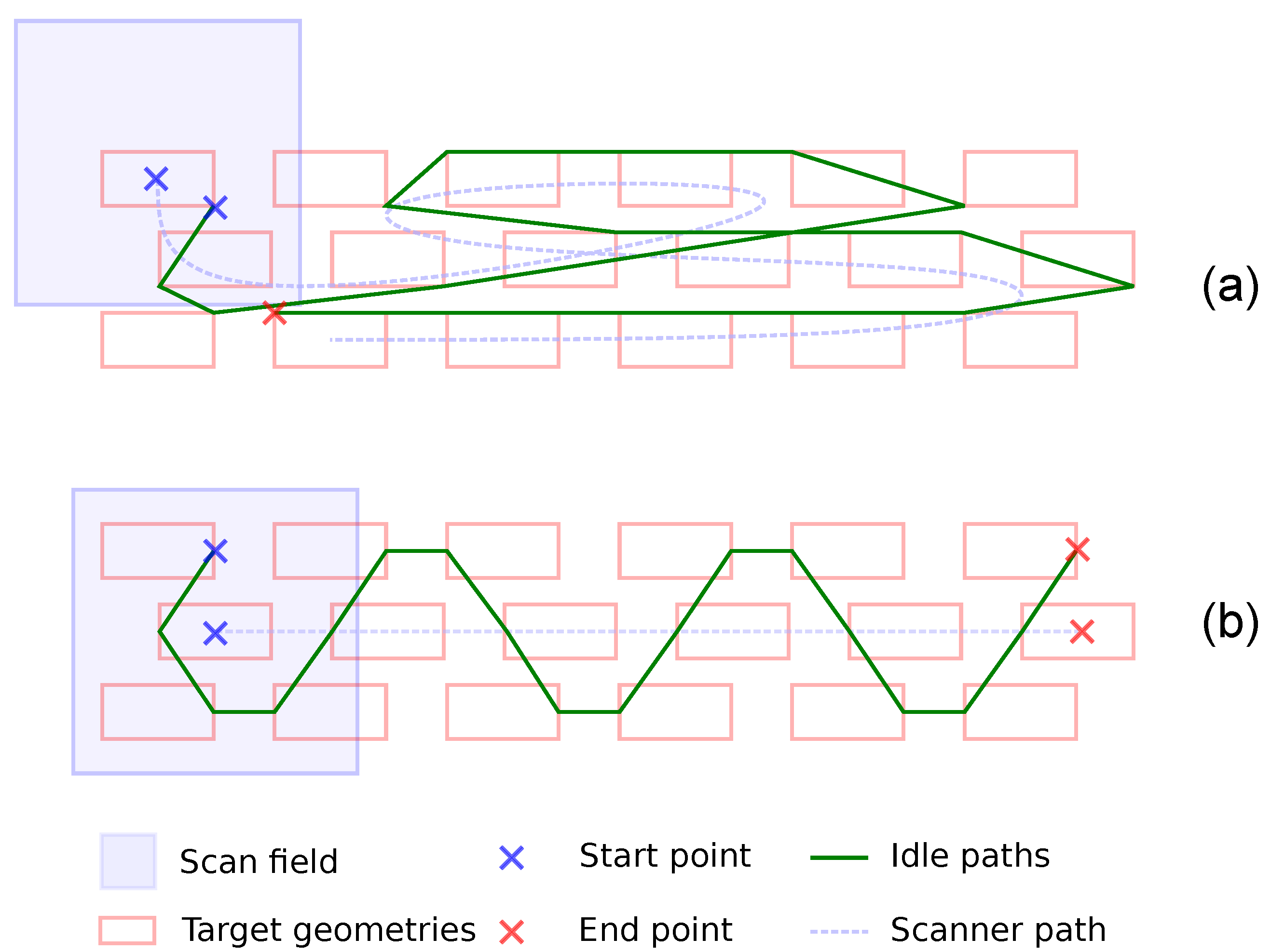
Figure 3.
Two feasible solutions for a CGTSP indicated by the yellow and green paths. The blue squares represent clusters, i.e. scan fields, which are labelled by black numbers. Shapes with a red outline represent SC, i.e. geometries. These are labelled by blue numbers.
Figure 3.
Two feasible solutions for a CGTSP indicated by the yellow and green paths. The blue squares represent clusters, i.e. scan fields, which are labelled by black numbers. Shapes with a red outline represent SC, i.e. geometries. These are labelled by blue numbers.
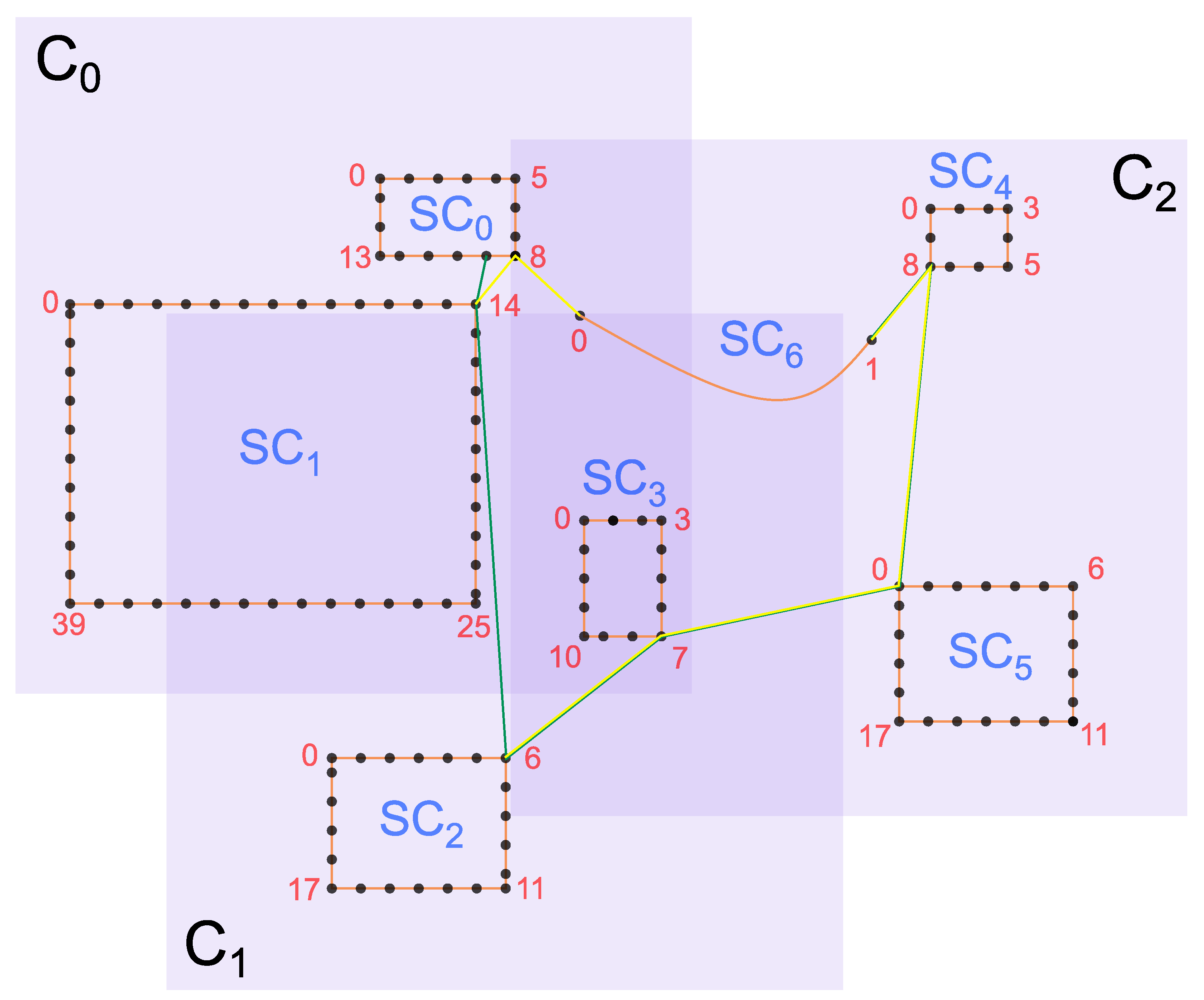
Figure 4.
Illustrates the steps of the scan field optimization process. a) depicts the imported geometries (red). b) depicts step one, the random creation of scan fields (blue) to cover all geometries. c) depicts the optimisation step, in which the area covered by the scan fields is minimised. d) depicts the optimisation step in which the scan fields are moved as far apart as possible. e) depicts the third optimisation step, in which the scan fields are centred over the respective geometries.
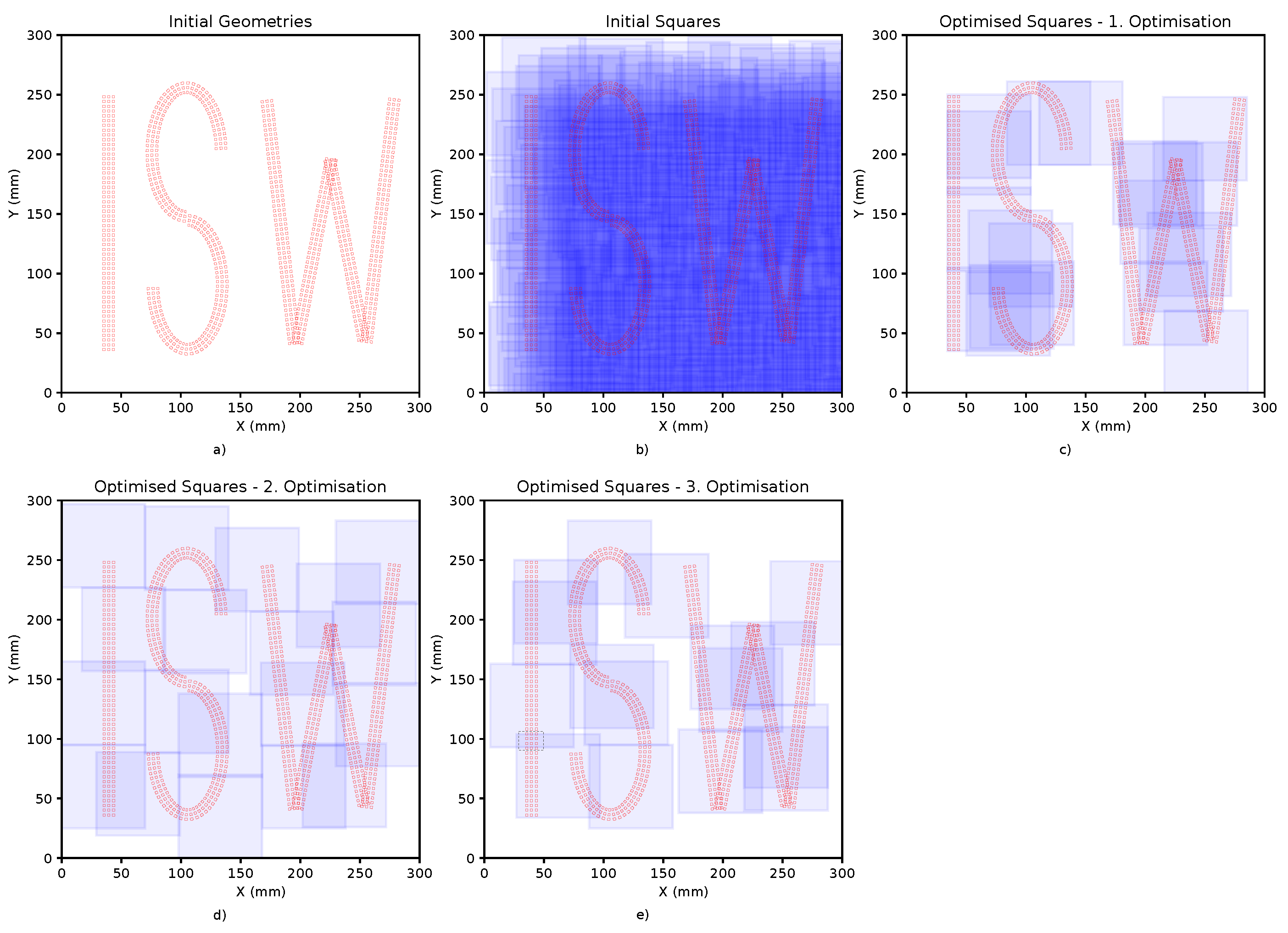
Figure 5.
An example for the additional penalty calculated for determining the processing order in a scan field. The green ’+’ are the centroids of the scan fields. The red ’+’ exemplifies one centroid of the other centroids relative to the current centroid of geometry zero. The blue ’x’: indicates the intersection of the path connecting two sequential scan fields with the boundary of the current scan field. It determines point ’B’. Point ’A’ is the normal projection of the centroid of an other geometry onto the path that connects two scan fields. The inverse of distance AB is added as a penalty for sequentially connecting geometry zero and one. The green doted line indicates the distance from B to the centre of each geometry.
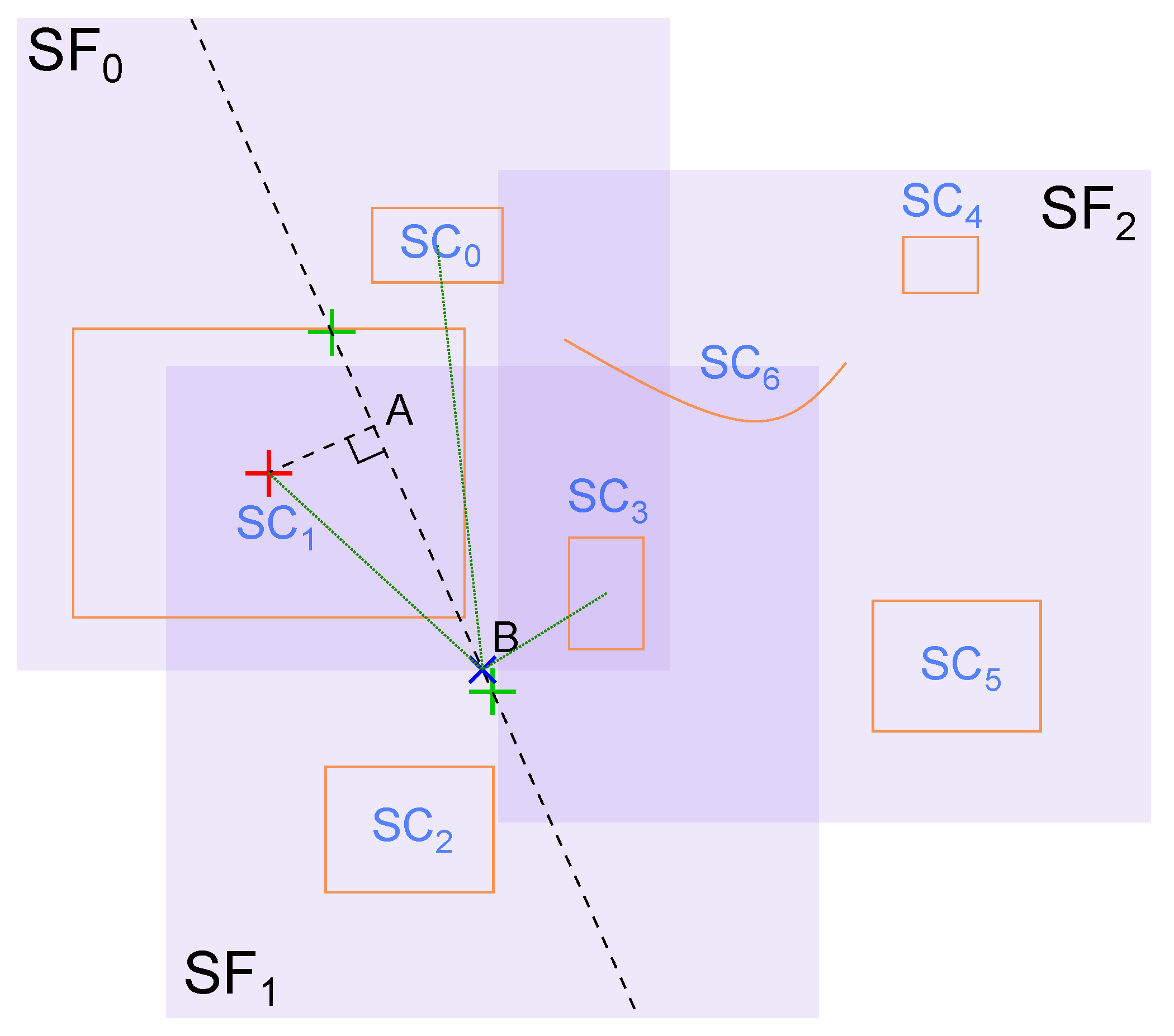
Figure 6.
Exemplary CAM results. The blue squares indicate the scan fields, i.e. cluster, the small orange squares are the geometries, i.e. SC, to be processed, and the green line is the resulting path that connects each geometry. The top result indicates good directionality of the TCP path, while the bottom result depicts bad directionality.
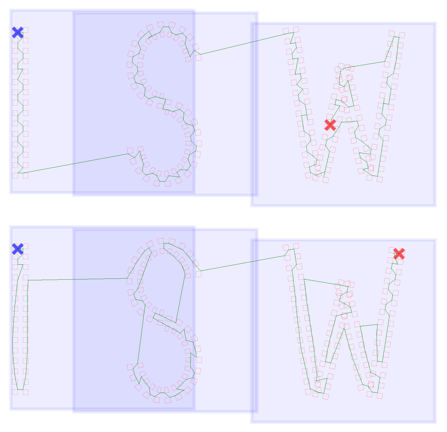
Figure 7.
Illustrates the process of the VEA a): The start-end vertex in (the first SC) is enhanced by choosing the red , which is closest to the vertex in the next SC. b): The red , which is closest to the line , is chosen as the new start-end vertex in . c): The red , which is closest to the line , is chosen as the new start-end vertex in . d): The start-end vertex in (the last SC) is enhanced by choosing the red , which is closest to the vertex in the previous SC. e): After verifying that no selected vertex can be further updated or improved, the VEA terminates, producing the enhanced start-end vertices for all SCs.
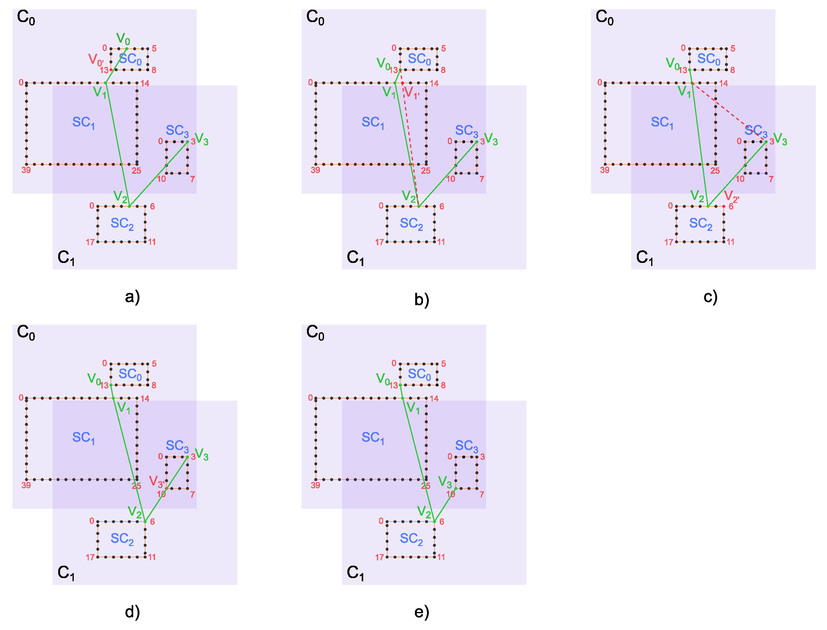
Figure 8.
Flowchart of hybrid genetic algoritm (HGA).
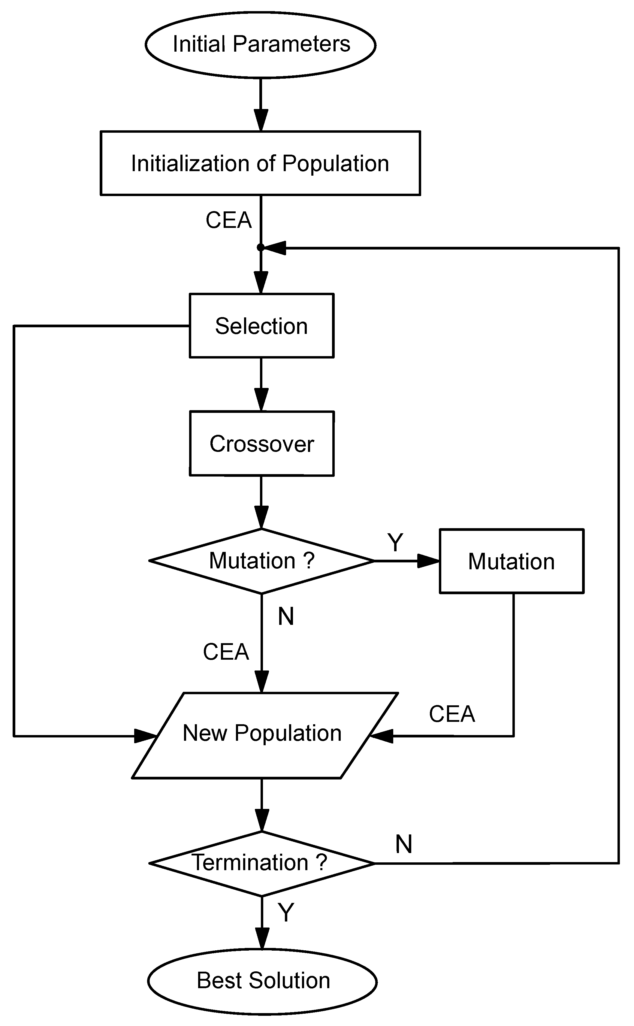
Figure 9.
Depiction of an exemplary result for the test case SC82C24 generated with the HHA algorithm. The start and end point are indicated by the blue and red ’x’, further results are to be taken from [32].
Figure 9.
Depiction of an exemplary result for the test case SC82C24 generated with the HHA algorithm. The start and end point are indicated by the blue and red ’x’, further results are to be taken from [32].
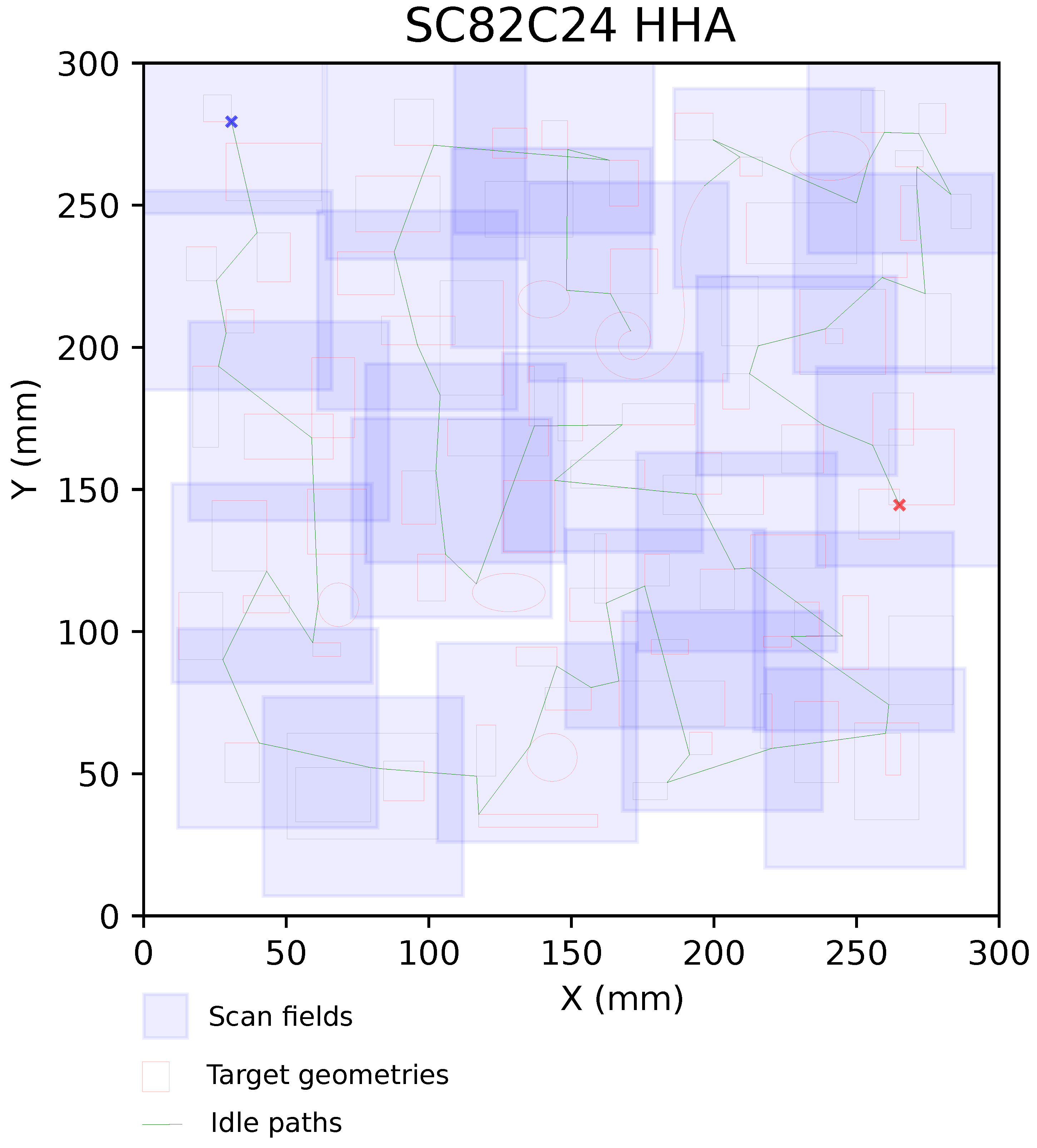

Table 1.
Computational time required using OR tools PCA to determine a path connecting different numbers of randomly placed scan fields. See sec:Discussion for details of the system used to perform the calculations.
Table 1.
Computational time required using OR tools PCA to determine a path connecting different numbers of randomly placed scan fields. See sec:Discussion for details of the system used to perform the calculations.
| Number of scan fields | calculation time (s) |
|---|---|
| 5 | 0.018 |
| 15 | 0.021 |
| 50 | 0.052 |
| 100 | 0.213 |
Table 2.
Results from ten calculations for each random pattern case.
| Type | HHA | HGA | Difference | ||||||
|---|---|---|---|---|---|---|---|---|---|
| Time ave. (s) | Idle stroke ave. (mm) | Idle stroke sd. (mm) | Time ave. (s) | Idle stroke ave. (mm) | Idle stroke sd. (mm) | Time (mm) | Idle stroke (mm) | ||
| SC32C2 | rnd. | 7 | 264 | 0 | 144.4 | 226.8 | 3.2 | 95.2% | -16.4% |
| SC82C24 | rnd. | 24.9 | 1692.8 | 45.6 | 901.9 | 1525.8 | 23.2 | 97.2% | -10.9% |
| SC122C4 | rnd. | 13.7 | 775 | 0 | 627.1 | 713 | 9.2 | 97.8% | -8.7% |
| SC278C18 | rnd. | 28.2 | 3025.6 | 52.5 | 1862.5 | 2877 | 37.8 | 98.5% | -5.2% |
| SC514C5 | rnd. | 29.3 | 1927.2 | 15.7 | 2855.5 | 1935.1 | 20.1 | 99.0% | 0.4% |
| SC946C32 | rnd. | 84 | 6701.2 | 84.4 | 14335.2 | 6642.9 | 76.3 | 99.4% | -0.9% |
Table 3.
Results from ten calculations for each ordered pattern case.
| Type | HHA | HGA | Difference | ||||||
|---|---|---|---|---|---|---|---|---|---|
| Time ave. (s) | Idle stroke ave. (mm) | Idle stroke sd. (mm) | Time ave. (s) | Idle stroke ave. (mm) | Idle stroke sd. (mm) | Time (mm) | Idle stroke (mm) | ||
| SC110C2 | ’O’ | 8.6 | 338.6 | 7.3 | 284.4 | 271.3 | 6.8 | 97.0% | -24.8% |
| SC200C3 | ’ISW’ | 13.2 | 702 | 0 | 573.4 | 618.1 | 11.9 | 97.7% | -13.6% |
| SC378C9 | ’O’ | 21.1 | 1101.3 | 32.9 | 3232.9 | 1054 | 4.9 | 99.3% | -4.5% |
| SC489C6 | ’ISW’ | 27.7 | 1489.7 | 31.5 | 3296.9 | 1530.7 | 32.5 | 99.2% | 2.7% |
| SC564C11 | ’O’ | 29.2 | 1613.3 | 23.3 | 7231 | 1592 | 17.7 | 99.6% | -1.3% |
| SC1017C16 | ’ISW’ | 53.7 | 3421.8 | 66.7 | 13813.8 | 3462.8 | 51.1 | 99.6% | 1.2% |
Table 4.
Results for the scan field optimisation, for twelve test cases [32], each test case was calculated 10 times.
Table 4.
Results for the scan field optimisation, for twelve test cases [32], each test case was calculated 10 times.
| Type | Nr. of scan fields ave. (mm) | Nr. of scan fields sd. (s) | Time ave. (s) | Time sd.(s) | Covered area ave. () | Covered area sd. () | Overlap ave. (%) | Overlap sd. (%) | |
|---|---|---|---|---|---|---|---|---|---|
| SC32C2 | rnd. | 2 | 0 | 9.3 | 1.6 | 7012 | 0 | 28.4% | 0% |
| SC82C24 | rnd. | 24.4 | 1.3 | 813.3 | 219.3 | 74630.1 | 1851.3 | 37.4% | 3.8% |
| SC122C4 | rnd. | 4 | 0 | 21.5 | 1.6 | 11671 | 0 | 40.5% | 0% |
| SC278C18 | rnd. | 19.2 | 1.2 | 1049.7 | 163.7 | 54868.8 | 1371.4 | 41.4% | 4.8% |
| SC514C5 | rnd. | 4.7 | 0.5 | 60.1 | 14.9 | 17725.2 | 55 | 22.2% | 8.5% |
| SC946C32 | rnd. | 33.1 | 1.5 | 4539.2 | 942.5 | 78331.7 | 1477.2 | 51.6% | 2.2% |
| SC110C2 | ’O’ | 2 | 0 | 6.1 | 0.4 | 7309.1 | 127.6 | 25.4% | 1.3% |
| SC200C3 | ’ISW’ | 3 | 0 | 11.4 | 1.0 | 11545.8 | 206.4 | 21.5% | 1.4% |
| SC378C9 | ’O’ | 8.3 | 0.5 | 123.7 | 26.8 | 33087.1 | 446.3 | 18.5% | 3.6% |
| SC489C6 | ’ISW’ | 6 | 0 | 92.0 | 36.1 | 16664.1 | 831.8 | 43.3% | 2.8% |
| SC564C11 | ’O’ | 11.4 | 0.5 | 276.0 | 57.1 | 44161.8 | 2453.0 | 20.7% | 6.6% |
| SC1017C16 | ’ISW’ | 16.1 | 0.6 | 894.1 | 236.1 | 55401 | 815.7 | 29.7% | 1.9% |
Disclaimer/Publisher’s Note: The statements, opinions and data contained in all publications are solely those of the individual author(s) and contributor(s) and not of MDPI and/or the editor(s). MDPI and/or the editor(s) disclaim responsibility for any injury to people or property resulting from any ideas, methods, instructions or products referred to in the content. |
© 2024 by the authors. Licensee MDPI, Basel, Switzerland. This article is an open access article distributed under the terms and conditions of the Creative Commons Attribution (CC BY) license (http://creativecommons.org/licenses/by/4.0/).
Copyright: This open access article is published under a Creative Commons CC BY 4.0 license, which permit the free download, distribution, and reuse, provided that the author and preprint are cited in any reuse.


