
Submitted:
14 November 2024
Posted:
15 November 2024
You are already at the latest version
Abstract
A Hybrid Artificial Neural Network (ANN) based constitutive model has been developed to predict the stress-strain behaviour of PET for the Stretch Blow Moulding process (SBM). The model has been created by combining a physical based function for capturing the small strain behaviour in parallel with an ANN based model for capturing the temperature dependant large strain nonlinear viscoelastic behaviour. The architecture of the ANN has been designed to ensure stability in a load-controlled scenario thus making it suitable for use in FEA simulations of stretch blow moulding. Data for training the model has been generated by a new semi-automatic experimental rig which is able to produce 850 stress strain curves over a wide range of process conditions (temperature range 95℃-115℃ and strain rates ranging from 1/s – 100/s) directly from blowing preforms using a combination of high-speed video, digital image correlation and sensors for pressure and force. The model has already been implemented in the commercial FEA package Abaqus via a VUMAT subroutine with its performance validated by comparing the prediction of the evolution of preform shape during blowing vs high speed images.
Keywords:
Numerical algorithms
; Multiaxial stress-strain behaviour
; Artificial Neural Network (ANN)
; Rate-dependent material
; Stretch Blow moulding
1. Introduction
Stretch Blow Moulding (SBM) is the most common method for producing Polyethylene Terephthalate (PET) bottles used in the carbonated soft drink (CSD) and water industries. The first step involves creating a preform, which is a test tube-shaped specimen made through injection molding. The preform is then heated above its glass transition temperature and shaped into a mould using both axial stretching through a stretch rod and radial stretching via internal air pressure. The typical evolution of the preform as it is stretched and blown in the mould is shown in Figure 1.
Manufacturers face a significant challenge in creating containers that utilize minimal material while still meeting the performance demands of in-service use, such as resisting top load, burst, and squeeze forces. Traditionally the optimum preform design and optimum process conditions have been determined by trial and error and knowhow, however the more modern approach involves the use of simulation whereby a finite element model of SBM is used to evaluate preform design and process conditions in advance. One of the key inputs into the SBM simulation is the material model that is required to accurately capture the nonlinear viscoelastic behaviour of PET subjected to high deformation and high strain rates at temperatures above the glass transition temperature (Tg). Previous work by the authors have demonstrated that a model originally developed by Buckley et al. [1,2,3] and with subsequent adjustments [4,5,6] can reasonably well capture this complex behaviour within SBM simulations. However the model has a limitation in the complexity of generating the material parameters which can be time consuming and expensive and it can have difficulty maintaining accuracy across a wide range of temperature and strain rates.
The aim of this paper is to develop an Artificial Neural Network (ANN) based constitutive model to predict the complex behaviour of PET in SBM. In order to do this, we will also present an experimental method for efficiently generating the rich data set required for producing a robust and accurate ANN model (850 strain-stress curves). Each strain-stress curves consists of more than 200 data points so that 253,864 data points can be collected during experiments. The work builds on previous publications [7,8] where authors demonstrated the ability of an ANN to predict the behaviour of PET biaxial stretched at different strain rates and temperatures for a simple displacement controlled planar experiment. In this paper we have increased the complexity and capability of the ANN model though the development of a new architecture enabling it to be used in the commercial finite element package Abaqus for complex load-controlled scenarios suitable for modelling the behaviour of PET in SBM.
For decades, researchers have been trying to develop accurate physical based models, which are able to describe the nonlinear viscoelastic behaviour of the PET during the SBM process at temperatures above the glass transition temperature (Tg). A comprehensive review of these approaches has been presented in our previous publication [7,8]. In summary, all of these approaches can capture the typical nonlinear temperature stress strain behaviour in specific conditions at different levels of accuracy. However, despite efforts to develop accurate models, weaknesses still exist due to the highly nonlinear deformation behaviour of PET during blow molding, which is affected by various parameters including temperature, deformation mode, stretch ratio, strain history, and strain rate. As pointed out by Menary et al., these parameters have a significant impact on the deformation behaviour of PET [9]. A shared characteristic among these constitutive models mentioned above is that they limit the depiction of the material's deformation behaviour to predefined parametric constitutive equations. However, fixed equations fail to accurately match the complexity of real conditions, as such physical models have associated inaccuracies. According to Liu et al. [10], the most obvious novelties of the ANN-based constitutive model is that it is able to build a complex nonlinear relationship in a form-free manner. As a result, the weakness of these models that depend on presumed functions with fixed mathematic expressions can be navigated by utilizing ANN technology.
In addition to the ‘form-free’ advantage mentioned above, the ANN also has other unique advantages compared with conventional physical models. Zhang et al. [11] demonstrated that a single neural network model was able to describe the behaviour of a material during deformation directly without any other equations, such as yield function, flow rule and hardening law. As a result, in comparison with a physical based model, the complexity of a constitutive model can be greatly reduced, which brings the dual advantage of reduced running time and coding simplicity.
One of the first researchers to propose the concept of an ANN-based constitutive model was Ghaboussi et al. [12]. They utilized an ANN-based constitutive model to forecast the stress-strain correlation of concrete when subjected to biaxial monotonic loading and uniaxial cyclic loading. Thanks to advancements in computer power, ANN-based constitutive models have undergone rapid development in recent years and have already found widespread use in various materials, such as foam [13], metals [14,15,16,17] and polymers [18,19,20].
Settgast et al. [13] proposed a hybrid ANN based model that embedded neural networks into the established framework of rate-independent plasticity and they demonstrated that this structure was able to simulate the elastic-plastic behaviour of foam efficiently. Settgast et al. [13] proved the fact that the ANN function can not only be used by itself but also that there were advantages in combining it with an existing traditional physical constitutive model. The cooperation with physical based functions not only reduced the size of training database required by training an ANN but also improved its stability.
Pandya et al. [14] upgraded Kessler’s model [21] and proposed a machine-learning based plasticity model which took strain rate and temperature into account. Li et al. [15,16] proposed an ANN based plasticity model to capture the large deformation response of the DP780 streel over a large range of strain rates and temperature. This ANN based model not only had higher accuracy and significant speed-up compared with the conventional plasticity model but also features a hardening law. Although Li ‘s previous work was in the metal domain, they demonstrated the feasibility of replacing conventional physical constitutive models by ANNs.
Diamantopoulou et al. [18] trained an ANN to describe the relationship among the process parameters, the degree of polymerization and the nonlinear stress-strain response of a polymer structure obtained from experiments. They highlighted the robustness of the developed ANN model and its advantage of reducing the complexity of the constitutive law. The hybrid modelling approach proposed by Jordan et al. [19] is taken by combing mechanism-based and databased model. However, their attention is limited to the stress-strain response for only uniaxial experiments and their temperature and strain rate range are relatively small (20℃ - 80 ℃ and 10-3/s -10-1/s) compared to the strain rates and temperature range required for modelling PET in SBM (1/s – 100/s and 85℃-115℃). Jang et al. [20] proposed a different combination method between FEA and ANN in that the ANN was only used to replace the nonlinear iterations in the stress return mapping method within a UMAT user subroutine [22].
The novelty of the current work can be summarised into two points. Firstly, an important point to note is that most of the ANN models discussed have been validated for displacement-controlled scenarios i.e. the boundary conditions for displacement are imposed on the model and the resulting force is calculated. We addressed this problem in our previous works [7,8] where we demonstrated the ability of the ANN to capture the nonlinear viscoelastic behaviour of PET for displacement controlled biaxial tests. However, to be used in a complex manufacturing simulation such as SBM, it is also important to validate the model in a load-controlled scenario i.e. a load is applied and the corresponding displacement is calculated. This is a more challenging problem since variables such as strain rate, mode of deformation are no longer fixed input parameters but are outputs from the model that vary at each time increment. In order to deal with this difficulty, a hybrid constitutive model combining advantages from both conventional physical based model and an ANN based model is proposed in the current work. The ANN part in the hybrid constitutive model adopts an innovative architecture specifically designed for load-controlled scenarios.
Another novelty of the current work is the acquisition system of experimental data. Generally, the experimental data required to train an ANN is acquired from standard specimens with simple graphs, for example, Jordan et al. [19] utilized dog-bone specimens and Li et al. [15] used flat smooth specimens with quasi-static strain rates. However, as highlighted by Menary et al. [9], the SBM process is a complex manufacturing process influenced by many dynamic parameters. As a result, in order to obtain an accurate enough ANN model, experimental data was collected from free stretch blow (FSB) experiments directly which are able to imitate real process parameters. All experimental data shown in the current work are published for the first time.
The paper is structured as follows. Section 2 describes the experimental procedure for generating the rich experimental data set necessary for training the ANN model. The component of the conventional physical based model used is described in Section 3 whilst Section 4 is utilized to introduce the detailed architecture of the hybrid ANN constitutive model. Subsequently, the hybrid ANN based model is trained in Section 5. Finally, in Section 6 the hybrid model is implemented in the finite element package Abaqus to simulate the behaviour of PET in a SBM simulation with the results validated against experimental data.
2. Experimental Procedure
2.1. Material and Specimens
The supplied PET material had an intrinsic viscosity of 0.81±0.02dL/g and a density of 1.33g/cm3, which is provided by DAK Americas for use in the current work. Further details on the material are available in previous work by the authors [7,8]. The drawing of the preform is shown in Figure 2 with all dimensions in millimetres.
2.2. Free Stretch Blow Test
A new robotic controlled test rig (Figure 3) has been developed by authors which is capable of automatically capturing stress strain data directly from a blowing preform as a function of process conditions (temperature, pressure, mass flow rate of air).
The test method consists of applying a pattern to a preform that is heated in an oil bath to provide uniform temperature (Figure 3 (b)) and subsequently blown without the constraint of a mould whilst the evolving preform shape and pattern evolution are recorded by two high speed cameras (Figure 3 (c)). The movement between the different stages is controlled by a robot (Universal R5) (Figure 3 (a)) and hence there is potential for automation.
The rig is instrumented with a pressure sensor and load cell in the stretch rod [23] which records the internal pressure and axial force on the stretch rod over time as the preform is blown (Figure 4 (a)). Digital Image Correlation (DIC) then produces a full-field strain map of the deforming surface of the preform whilst the pressure and force data can be converted to stress using thin-walled membrane theory [24]. With the help of the stretch rod device and the 3D DIC technology, the stress-strain/stretch ratio data for every point on the preform can be calculated (Figure 4 (b)).
Figure 5 shows a typical image of the blowing preform as recorded by the high-speed cameras with the contours representing the hoop strain whilst Figure 6 shows the influence of temperature on the evolution of force and pressure for a preform, recorded by the pressure sensor and load cell shown in Figure 4(a).
Stress-strain curves are available for every pixel in the DIC analysis providing hundreds of stress strain curves for each process condition. In each free flow experiment, 85 strain-stress curves are selected from experiments corresponding to different pixels and they will be used as a training database in the future. Figure 7 shows an example of the stress-strain curves produced at three different locations along the length of the preform for a preform blown at 115℃ and a pressure of 8 bar, thus highlighting the influence of strain history/deformation mode on the material behaviour. The three locations are known as the upper point, middle point and the lower point. The three positions on the preform are defined in Figure 2. An example of stress-strain curves in the both hoop direction (a) and axial direction (b) taken from the midpoint of the preform for different preform temperatures is shown in Figure 8 It was worth noting that all experiments were repeated three times and the values of stress and strain were averages of these three experimental values.
The rig is ideal for efficiently producing a rich data set covering a wide range of process conditions directly relevant to SBM and is therefore suitable for producing data that can subsequently be used to train an Artificial Neural Network (ANN) to model its behaviour.
A series of experiments were carried out by using a mixed level full factorial design of experiments (DoE) with 2 factors – temperature and mass flow rate of air entering the preform. Due to its known importance on the behaviour, the temperature was discretised into 5 levels ranging from 95℃ (just above the glass transition temperature) to 115℃ (just below the cold crystallisation temperature). The mass flow rate was discretized into two levels (low and high). As a result, there are 10 different experiments (also known as 10 DoEs) involved in the current paper, as shown in Table 1. Each experiment (DoE) was repeated three times. The average values of stress and strain obtained from these three experiments were treated as experimental values of this DoE and were used to train the model. As mentioned above, 85 strain-stress curves are selected from one free stretch blow experiment corresponding to different heights along the preform and our experiment equipment is able to record stress and strain values every 0.0005s during the free stretch blow experiments.
The mass flow rate of air was controlled by adjusting a flow restrictor valve, as shown in Figure 9.
The high mass rate means that the rotating knob is set as flow index ‘6’ as shown in Figure 9 and the low mass flow rate corresponds to the flow index ‘2’ on the rotating knob which indicates ‘nearly closed’. Based on calculation of Salomeia et al. [25] the low flow setting corresponds to a mass flow rate of 8.88±0.195 g/s whilst the high flow rate corresponds to a mass flow rate of 33.96±0.863 g/s. The flow rate of air effectively controls the rate of inflation of the preform and hence influences the strain rate of the deforming material. The stretch rod displacement and velocity were set at fixed values of 130 mm and 0.5 m/sec respectively for all experiments whilst the valve for enabling the air to enter the preform was opened at the same time when the stretch rod touched the tip of preform (known within the bottle blown industry as P0).
3. Brief Description of Buckley Model
Menary et al. [26] compared several physical based models, including a hyperelastic model, a creep model and the Buckley model, to ascertain their suitability for modelling stretch blow molding. The model proposed by Buckley et al. [1,2,3] was found to provide the simulation results that match best with the experimental data. After Menary’s work, the model has evolved to capture key features of the behaviour of PET including how the onset of strain hardening changed as a function of temperature and strain rate [4,5,27]. A 1D representation of the Buckley is shown in Figure 10 which shows a parallel circuit with two arms, named the bond stretching part and the conformation part respectively.
The bond-stretch arm represents the bond deformation of the polymer, exhibiting the instantaneous stress from the interactions of the molecular bonds and is important for predicting the onset of yield and how it varies with temperature and strain rate. In the conformational arm, it represents the perturbation of the polymers conformation and is determined by the change in an entropic free energy function. The conformation part captures the large strain behaviour post yield including strain softening and strain hardening and how these change as a function of temperature, strain rate and mode of deformation.
The Buckley model can be expressed by Equ(1),
where is the principal bond-stretching stress and is the principal conformation stress.
3.1. Bond Stretching Part
The principal deviatoric stress of the bond-stretching component () is expressed by Equ (2),
where is the contribution to shear modulus arising from bond stretching, is the relaxation time and is the deviatoric true strain. In the present work, is set as 600MPa [1]. In order to obtain , three equations are utilized, including Eyring formulation [28], Vogel-Tammann-Fulcher function [29,30] and Arrhenius equation [31].
According to Li & Buckley [32], an implicit method or identified integral solution for Equ (2) can cause potential numerical difficulty in modelling large and post-yield deformations. In order to solve this problem, an explicit method was proposed to solve from Equ (2) , as shown in Equ (3) and Equ (4), which have been subsequently used in the VUmat subroutine developed in the current work.
is the time increment, is the spin tensor and is the stress increment in this time increment. is obtained from Equ(4).
3.2. Conformation Part
In the conformational part, the stress component () is represented by the crosslinks-sliplinks model proposed by Edwards and Vilgis [33]. The principle conformational stresses () are expressed by Equ (5),
where is the hydrostatic stress, is the determinant of the deformation gradient tensor, is the principal stretch and is obtained from the free energy function which was derived by Edwards and Vilgis [33] as shown in Equ (6),
where is the entanglement density, is the Boltzmann’s constant, is the absolute temperature, is the looseness parameter of the entanglement, are the principal network stretch, and is a measurement of the inextensibility of the entanglement network where the maximum extension is determined by .
Adams et al. [3] updated Equ (5) by considering the entanglement slippage in the conformational part to capture the strain hardening behaviour more accurately. As a result, the total stretch () in Equ (5) is replaced by the slippage stretch (), which can be obtained by Equ (7),
where are the deviatoric stresses of the conformational part and is the slippage viscosity as shown in Equ (8),
where is the maximum principal network stress, is the critical value of network stretch and is the initial viscosity.
Yan [4] modified Equ (8) by changing from a constant to a function with respect to temperature and strain rate, as shown in Equ (9),
where is the shifted temperature obtained by Equ (10),
where is the shift factor which is the ratio between the shifted temperature and the reference temperature, is the strain rate and is an indicator of deformation mode.
4. Hybrid ANN Based Constitutive Model
4.1. Algorithm Selection and Overall Architecture Selection
There are lots of typical algorithms and neural network architectures which can be used to train an ANN based constitutive model. According to Zhang et al. [34], the most widely used machine learning (ML) algorithm for modelling stress-strain relationship in the soil domain is a backpropagation neural network (MULTI-LAYER PERCEPTRON). Zhang et al. [34] also proposed that the wide application of the Multi-layer Perceptron was due to its relatively simple structure and strong non-linear mapping ability which was also demonstrated by Hagan et al. [35] and Mehrpouya et al. [36]. The feasibility of combining the Multi-layer Perceptron with finite element code has already been demonstrated by Kessler et al. [21], Lefik et al. [37] and Hashash et al. [38]. Since the Multi-layer Perceptron has already been applied successfully for modelling non-linear material behaviour in Abaqus, it is also adopted in the current work.
The aim of the model in the current paper is to predict the non-linear viscoelastic behaviour of PET above Tg subjected to large deformation. The initial approach was to try and implement an ANN model only without any constitutive equations. However whilst this approach worked reasonably well for displacement controlled simulations as demonstrated in the authors’ previous works [7,8], it was found that the model became unstable when applying it to load controlled simulations. There was a significant problem in the regions of small strain at the beginning of the analysis where the magnitude of the error for the stress prediction from the ANN was of the same order as that of the magnitude of the stress. To avoid this phenomenon some physically based equations had to be used in conjunction with the ANN to create a Hybrid ANN.
Similar concepts of combining ANN models with physical models have already been proposed and demonstrated by several researchers, such as Pandya et al. [14] and Jordan et al. [19]. Pandya et al proposed. [14] an isotropic hardening term kSV obtained from the mixed Swift-Voce law to help the ANN model to take isotropic hardening into account and Jordan et al. [19] utilized a temperature-dependent Hooke law to help the ANN based model to describe the elastic behaviour. Inspired by these hybrid ANN based models, the Bond stretching part described by Equ (2)-(4) is retained for a hybrid model in the current work thus ensuring reasonable predictions in the initial small strain regime of the model and thus reduce the effect of error propagations. The architecture of the hybrid ANN model is shown in Figure 11.
As shown in Figure 11, the conformation part from the original Buckley model is replaced by two ANNs, named as ‘ANN_Temperature’ and ‘ANN_Strain history’. The ‘ANN_Temperature’ component predicts the conformational stress dependent only on the stretch in the axial and hoop direction whilst the ‘ANN_Strain history’ will shift this prediction depending on the strain history experienced to date by the element. The details of ‘ANN_Temperature’ and ‘ANN_Strain history’ will be presented in Section 4.3, 4.4 and 4.5.
Despite the wide range of experimental process conditions shown in Table 1, it is inevitable that there will be a range of stretch ratios and strain rates not covered in the training data, in other words, it is impossible to collect all ‘strain history’ data that might occur during simulation process from experiments. This could lead to scenarios that the ANN model is operating in regions where it has not been trained causing instabilities and errors in the model. In order to deal with this issue, this two-step ANN architecture including the ‘ANN_Temperature’ and the ‘ANN_Strain history’ was proposed and we adopt this strategy during practical simulation process that if an input variable of the ‘ANN_Strain history’ exceeds the training range value, it will be limited to the maximum or minimum available from the data and keep the ‘ANN_Temperature’ operates in the region where it has been trained all the time. As mentioned above, the ‘ANN_Temperature’ contributes most of the output of this two-step ANN architecture and the ‘ANN_Strain history’ only provides shift-factors. As a result, this two-step ANN architecture offers superior stability compared to the one-step method.
The ANN part of the model shown in Figure 11 is in parallel with the bond stretching part and operates independently. Therefore, the total stress() can be described by Equ(12),
As a result, in order to obtain (required to train the ‘ANN_Temperature’ and ‘ANN_Strain history’), the ‘Bond stretching part’ needs to be calculated and subtracted from the total stress, which is equal to experimental true stress values collected from the free stretch blow experiments (SBM) described in Section 2.
4.2. Calculation of Bond Stretching Stress
A detailed procedure of the characterization of ‘Bond stretching part’ can be found in Buckley’s previous works [1,3].
According to the relationship between true strain and true stress at yield points and deformation temperature, the shear (Vs) and pressure (Vp) activation volumes can be calculated, which are critical variables in the ‘Eyring process’. Another variable in the bond stretching part is the limiting viscosity (μ0) which is temperature dependent to predict the temperature effect on the yield stress. Once the limiting viscosity(μ0) is defined, the reference viscosity(μ0*), limiting temperature (T∞) and the viscosity constant (Cv) can be calculated. By using the characterized values of Vs, Vp, μ0*, T∞ and Cv, the equations belonging to the ‘Bond stretching part’ are all prepared well. Detailed material constants used in ‘Bond stretching part’ can be found in Appendix A.
An example of the relationship between principal bond-stretching deviatoric stress (Sb) and principle conformational deviatoric stress (Sc) is shown in Figure 12. This example was exported from free stretch blowing experiment at 100℃ and the inside pressure of preform was set up as 8 bar (P8N6T100 in Table 1).
According to Figure 12(c)(d), it can be observed that Sb contributes significantly to the total stress at the beginning of deformation, particularly, when the stretch is smaller than 1.02. However, with the development of stretch, the value of Sb decreases rapidly and approaches zero as the stretch increases and is subsequently dominated by the conformational part as shown in Figure 12(a) and Figure 12 (b). In the current work, the conformational part will be replaced by the ANNs.
In conclusion, although the ‘Bond stretching part’ exists in the Hybrid ANN based constitutive mode shown in Figure 11, it only contributes stress value at the beginning of the SBM process, especially it operates independently from the ‘ANN part’.
4.3. ANN_Temperature
The architecture of the ‘ANN_Temperature’ is shown in Figure 13. The number of layers and the number of neurons in each layer will be introduced in the next section (Section 5).
The inputs to the model are chosen to reflect the most important parameters that influence the behaviour of the material. ‘Stretch_axial’ and ‘Stretch_hoop’ represent the principal stretches in the axial and hoop direction respectively whilst ‘Stress_ANN(axial)’ and ‘Stress_ANN(hoop)’ are the predicted stresses by the ‘ANN_Temperature’ in the axial and hoop direction respectively. Our previous works [7,8] has already demonstrated that one multi-layer perceptron is able to accurately describe the relationship between strain, stress and other variables therefore the ‘ANN_Temperature’ also adopts a conventional architecture of a multi-layer perceptron. The detailed transfer functions, weight matrices and bias vectors definition were also explained in our previous work [7,8]. Note strain rate is not an input parameter to this ‘ANN_Temperature’ component so the prediction from the ‘ANN_Temperature’ is independent of this variable and is therefore the best fit prediction at the given temperature across all of the experiments conducted at different strain rates.
4.4. ANN_Strain History
It has been demonstrated experimentally that strain rate has an important influence on the behaviour of PET above Tg during biaxial tension experiments [1,3]. However, the influence of strain rate decreases in the SBM process. The strain rate during SBM process is mainly influenced by the mass flow rate of air and the temperature of preform. The maximum strain rate appearing in every free stretch-blow test in Table 1 was recorded and is shown in Figure 14.
The ‘low flow rate’ in Figure 14 represents the ‘flow index 2’ shown in Table 1 and the high flow rate represents the ‘flow index 6’. According to Shiyong [4], the strain rate mainly influences the behaviour of PET during the SBM through the ‘self-heating’ phenomenon and Shiyong also proposed an empirical equation to roughly quantify the influence produced by the high strain-rate.
As shown in Figure 14, the difference on maximum strain rate is most obvious when the oil bath temperature is 110 ℃ so that the ‘110℃ scenario’ is also be adopted in current work as an example. Shiyong [4] proposed a concept called ‘equivalent temperature’ in his previous research, which is able to quantitatively transfer the influence produced by high strain-rate to the effects provided by temperature. As shown in Figure 15, according to Shiyong’s empirical equation, the behaviour of PET (strain-stress curve) stretched at nominal strain rate 128/s and 110℃ is similar to the behaviour of PET (strain-stress curve) stretched at nominal strain rate 1/s and 131℃. It can therfore be observed that the influence of the strain rate on the PET decreases with the increase of the strain rate. The equivalent temperature of 75.6/s and 107.6/s are 129.2℃ and 130.4℃. The difference between 129.2℃ and 130.4℃is so inappreciable that this difference can be ignored. As result, comparing with the biaxial stretching experiments, the strain rate is not as much as important in the SBM process since it mainly operates in the high strain rate range even the ‘flow index’ has already been adjust to only 2. As a result, the influence of the strain is removed from the main ANN (the ‘ANN_Temperature’).
Gorji et al. [39] proposed an equation when developing a neural network model for large deformation of metals, which is shown in Equ (12). This equation will be used in the ‘ANN_Strain history’ component of the model in this work. The equation effectively captures the stretch experienced by the material ( at a specific instance in time (.
According to Gorji et al. [39], due to the integration operation, the variable obtained in Equ (13) is also able to capture the strain-path experienced by the element during simulation so that this variable is named as ‘strain history’ in this paper and it is much more stable than using the stretch at a given time increment directly as it is less susceptible to fluctuations. The integration operation will also bring an addition advantage when this variable is used in ANN model that it is able to change a typical multi-layers perceptron to a kind of dynamic model to reduce oscillations efficiently because the ‘strain history’ is a historical variation of the inputs (the stretch() used in Equ (13) is the main input variable of the ‘ANN_Temperature’, as shown in Figure 13). This advantage is able to avoid the current hybrid ANN based constitutive model exhibiting strong oscillations, which is a typical disadvantage of multi-layer perceptrons.
As shown in Figure 2, three different sampling points are selected on the wall of preform, named as upper point, middle point and lower point. During experiments, stress and strain data in both axial and hoop directions were collected respectively for these three sampling points. To combine the data from both directions (axial and hoop direction), the concepts of equivalent stress and equivalent strain (von Mises strain) were adopted in the current paper. The relationships between equivalent stress and equivalent strain of these selected samplings are shown in Figure 15,
where equivalent strain () and equivalent stress () are obtained by Equ (13) and Equ (14)
According to Figure 16, it can be observed that the behaviour of PET varies depending on the location of the selected element on the preform even in the same free stretch experiment because different position means these three sampling points have undergone different strain histories.
The development of ‘strain history’ (obtained by Equ (12)) of these selected sampling points vs equivalent strain are shown Figure 17. When comparing Figure 17 with the stress-strain behaviour in Figure 16, it can be observed that the ‘strain history’ is a suitable input variable to be used in an ANN based constitutive model since (i) it has more direct correlation with the stress-strain curve and (ii) it is has a more stable evolution.
The structure of the ‘ANN_Strain history’ is shown in Figure 18. The number of layers and the number of neurons in each layer will be introduced in the next section (Section 5).
‘Stress_ANN(axial)’ and ‘Stress_ANN(hoop)’ are inherited from the ‘ANN_Temperature’ and they share the same values. As mentioned above, ‘Strain_history(axial)’ and ‘Strain_history(hoop)’ represent the ‘strain history’ of the axial and hoop directions separately which are calculated by Equ (13). ‘Shift-factor(axial)’ and ‘Shift-factor(hoop)’ are factors required to shift the prediction of stress from ‘ANN_Temperature’ allowing for the effect of strain history.
An example is shown in Figure 19(a) where the outputs of the ‘ANN_Temperature’ for the upper point and the lower point of the preform are both the same and is shown by the yellow curve because they share the same temperature (locations of ‘upper’ and ‘lower point’ can be found in Figure 2). With the help of the ‘ANN_Strain history’ or the shift-factor, the equivalent stress- equivalent strain curves for the upper point and the lower point are separated because the ‘strain history’ of these two points is different which brings different shift-factors, as shown in Figure 19(b). The concept of tuning the output of the ANN with extra factors was inspired from the work of Pandya et al. [14], who applied an isotropic hardening term kSV obtained from the mixed Swift-Voce law to adjust the result from the ANN to reflect the influence of isotropic hardening. In other words, ‘ANN_Strain history’ is fine-tuning the outputs from the ‘ANN_Temperature’ to take the influence of strain history into account.
4.5. A Walk-Through of the Hybrid ANN Based Constitutive Model
The detailed flow chart for calculating the stresses using the Hybrid ANN based constitutive model is shown in Figure 20. The entire constitutive model can be separated into two parts, Bond stretching part and ANN part. The explanation on ‘Bond stretching part’ can be found in Buckley’s previous works [1,3]. As a result, the detailed calculating procedures of this part is not included in the current paper. According to Figure 20, in order to obtain ‘Stress_ANN(axial)’ and ‘Stress_ANN(hoop)’, the ‘Stretch_axial’ and ‘Stretch_hoop’ are firstly input into the ‘ANN_Temperature’ introduced in Section 4.3. It is worth noting that ‘Stress_ANN(axial)’ and ‘Stress_ANN(hoop)’ are not only input variables of ‘ANN_Strain history’ introduced in Section 4.4 but also used in the equation for calculating the ‘Final stresses’. As explained in Section 4.4, in order to take the effect of strain history into account, ‘Shift-factor(axial)’ and ‘Shift-factor(hoop)’ need to be multiplied with the prediction of stress from ‘ANN_Temperature’ (‘Stress_ANN(axial)’ and ‘Stress_ANN(hoop)’). The ANN part and the ‘Bond stretching part’ are added together as defined in Equ(12) to obtain the final stress of the Hybrid ANN based constitutive model.
5. Training ANN Part of the Constitutive Model
It is worth noting that experimental data of P8N2T110 and P8N2T115 shown in Table 1 have already been removed from the experimental database before the training procedure because they are used to validate the performance of the Hybrid ANN based constitutive model in Abaqus. Detailed content is indicated in Section 6.
As mentioned above, each experiment shown in Table 1 is able to provide 85 strain-stress curves so that the experimental database actually includes 680 strain-stress curves. In line with work conducted by Hagan et al. [35], 85% of these strain-stress curves are selected for training the ‘ANN_Temperature’ and the ‘ANN_Strain history’. As a result, for each experiment, 8 complete strain-stress curves are classified into the testing database and others belong to the training database. For these 8 curves, 6 curves were selected randomly and the complete strain-stress curves of the upper point and the lower point are compulsorily included in the testing database.
5.1. Detailed Training Settings
The neural network was initially built, trained and validated using the MATLAB neural network toolbox.
The ‘ANN_Temperature’ shown in Figure 13 is a typical multilayer perceptron. A similar ANN architecture with 3 layers was adopted by Tao et al. [40]. They utilized this ANN to establish a relationship between in-plane strains and corresponding stiffness matrix in an Umat subroutine in Abaqus. Since the number of input and output variables, the size of the experimental database and the complexity of the function are all similar, the number of layers used by Tao was also used in this model.
Le et al. [41] proposed that an ANN should use as few neurons as possible on the premise of ensuring accuracy during training and they demonstrated the performance surface of an ANN with simpler architecture is smooth and monotonic, and thus is more suitable to describe a physical phenomenon. In order to avoid overfitting and unrealistic performance surface with localized, inconsistent fluctuations, the number of neurons in each layer is set at 9, a relatively small value that was determined after trial-and-error testing. The ‘ANN_Temperature’ architecture is defined by the nomenclature [3,9,9,9,2], which indicates that the ANN has three input variables, two output variables, and three hidden layers with each layer having 9 neurons. The training epoch was set up as 1000.
The details on the training algorithm selection (Bayesian regularization backpropagation algorithm) and trial-and-error testing for the ‘ANN_Temperature’ can be found in our previous works [7,8]. A detailed work flow on how to train an ANN by experimental datasets from the materials domain is described by Pal et al. [42] whilst information about the training algorithm and regularization have already been explained by Kim et al. [43].
The training program and algorithm used by the ‘ANN_Strain history’ is the same as the ‘ANN_Temperature’ described above. After the same trial-and-error testing, the structure of the ‘ANN_Strain history’ is defined as [4,4,5,5,2], meaning the ANN has four input variables, two output variables and three hidden layers of 4, 5 and 5 neurons respectively.
It is worth noting that all training data need to be normalized before training these two ANNs (ANN_Temperature & ANN_Strain history ). The magnitude of all training data is scaled equally into the interval of (-1,1) and re-normalization on their outputs is also necessary. The ‘normalization’ and the ‘re-normalization’ procedures are controlled by the algorithm automatically and therefore exceeds the scope of this article.
5.2. Validation in Testing Database
Once both the ‘ANN_Temperature’ and the ‘ANN_Strain history’ are trained well, the entire ‘ANN part’ (‘ANN_Temperature’ with the help of the ‘ANN_Strain history’, as shown in Figure 11) will be validated via the testing database to verify the accuracy of training procedure. This operation is implemented in Matlab. As mentioned above, the complete strain-stress curves of the upper point and the lower point are compulsorily included in the testing database. Therefore, the performance of the entire ‘ANN part’ when simulating the PET behaviour at the ‘upper point’ and the ‘lower point’ position is shown in this section.
In order to quantify the accuracy of the ANN models, the results shown in Figure 20 are evaluated by both the Mean Square Error function (MSE) and the Mean Relative Error (MRE), which are obtained by Equ (15) and (16) respectively.
is the simulation stress value of each data point, is the corresponding experimental data and is the total amount of data points.
Figure 21.
testing results of the Hybrid ANN based constitutive model for testing database from Table 1 on the upper and lower points of the preform.
Figure 21.
testing results of the Hybrid ANN based constitutive model for testing database from Table 1 on the upper and lower points of the preform.
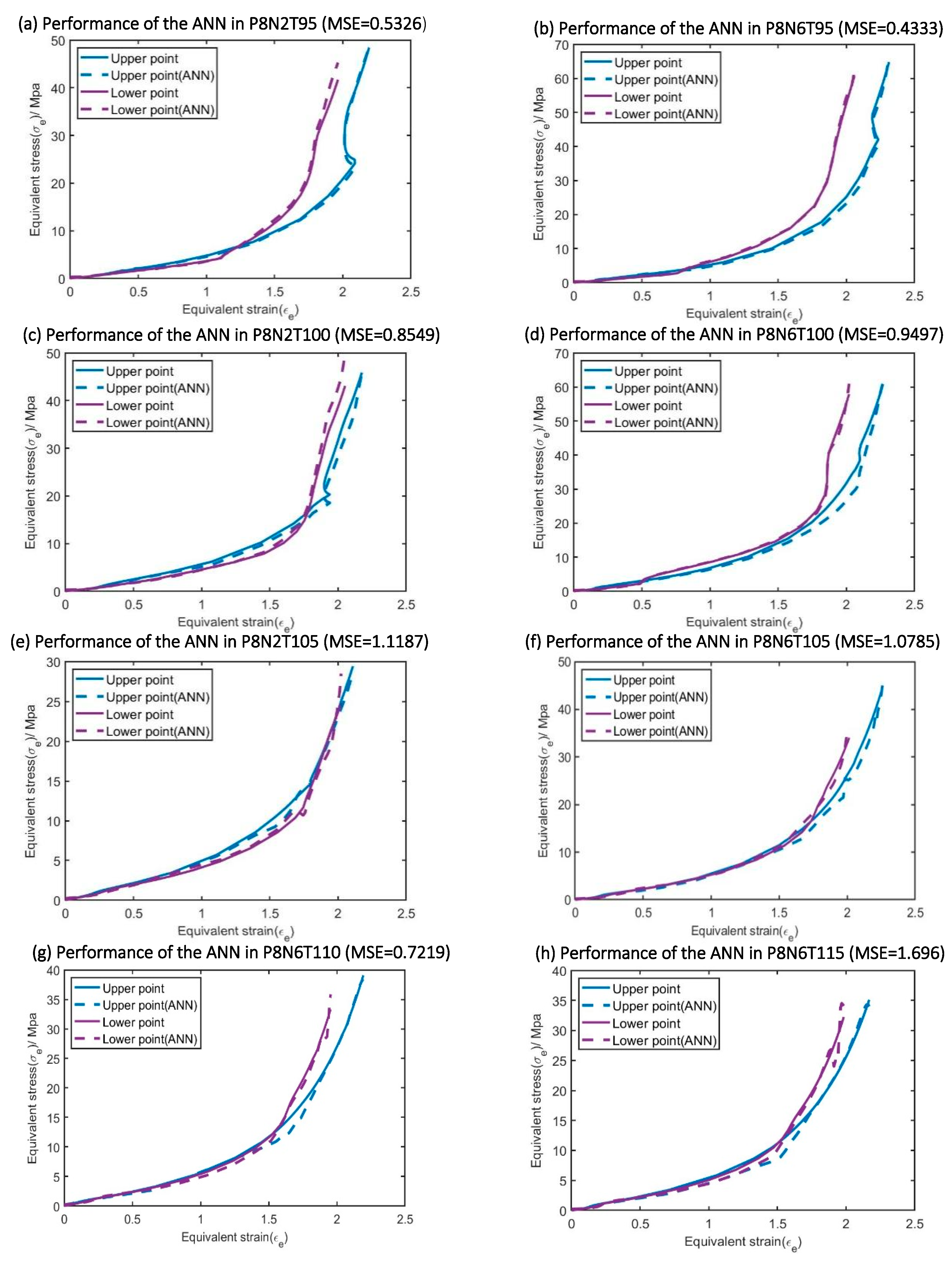
According to Figure 20 and Table 2, ‘ANN_Temperature’ and ‘ANN_Strain history’ have accurate performances when they are used to predict the stress output of data in the testing database. As a result, the training process of both ‘ANN_Temperature’ and ‘ANN_Strain history’ can be considered as accurate enough for the current work.
6. Validation and Comparison
6.1. Implementation in Abaqus
The Hybrid ANN based model was implemented in Abaqus by a VUmat subroutine. PET’s material properties were defined by density (1.33g/cm3) and Poisson’s ratio (0.495). Due to the ratio of thickness to radius in the bottle, the stress through the thickness can be neglected and shell elements can be used. Given the axisymmetric nature of the preform geometry, an axisymmetric shell (known as SAX1 in Abaqus) was adopted during validation. The preform as shown in Figure 2 has been meshed with 80 SAX1 elements with each element assigned a corresponding thickness. The preform is constrained in the axial direction at the position just after the neck support ring and is constrained in the axial direction at the preform tip. Similar to Nixon et al. [44], a fluid cavity is setup inside the preform to model the different mass flow rates of air entering the preform for each experiment with a fluid exchange property applied to represent the flow of air from the compressor to the preform. Non-deformable items such as the stretch-rod and preform clamp were modelled using rigid elements (RAX2). The detailed model of free stretch blow process used in Abaqus is shown in Figure 22.
The Hybrid ANN based constitutive model in the current paper is developed for simulating the SBM process specifically. Compared with the strain-stress curve of PET at some specific positions, the industry takes more care of the accuracy of the final geometry of the preform predicted by the Hybrid ANN constitutive model because it has a directly relationship with the final product of the SBM process. In order to quantitatively compare these preforms’ geometries predicted by the Buckley model and the Hybrid ANN model respectively in the following section, a concept called ‘average nodal distance’ was proposed, its schematic diagram and calculation equation are shown in Figure 23. As shown in Figure 23, the middle layer outline of the preform collected from the experiment is represented by the red dotted line, while the corresponding simulation result is shown by the green dotted lines. Figure 3(c) indicates the relative positional relationship between high-speed cameras and the preform during experiments. These two cameras are placed horizontally at the middle of preforms during experiments so that it cannot capture the evolution of strain for these positions located at the top and bottom of the preform due to the angle issue. This is the main reason why the middle layer outline (red solid line) is missing at the bottom of Figure 23. In other words, the ‘strain’ variable for some nodes in the simulation model do not have corresponding experimental data. These nodes which have experimental ‘strain’ data collected by these two high-speed cameras are shown by the blue dotted line in Figure 23. And these two nodes which share the same position in the simulation model and the preform sample at be beginning of free stretch blow process are called one ‘node pair.’ The variable ‘average distance’ is obtained from these ‘node pair’.
6.2. Free Blow Validation
As mentioned above, experimental data of P8N2T110 and P8N2T115 have been removed from the training database. Therefore, test conditions of P8N2T110 and P8N2T115 are used to validate the performance of the Hybrid ANN based constitutive model in Abaqus/Explicit in the current section.
According to Section 4, the Hybrid ANN based model is developed from the Buckley model. Therefore, the evolution of the preform as predicted by the Hybrid ANN based constitutive model and the Buckley model developed by Shiyong [4] at different time moments are shown in Figure 23 and Figure 24 respectively. MATLAB is used to plot these geometries via coordinate data of all elements which is exported from Abaqus/Explicit. The outline of the preform captured by the DIC analysis during the free stretch blow experiment is represented by the red dotted line, while the simulation results by the Buckley model and the Hybrid ANN-based model are shown respectively by the blue and light blue dotted lines.
In order to show the whole process clearly, each entire free stretch blow simulation is represented by 3 pictures which are recorded at different time moment and these three diagrams divide this process as equally as possible, for example, the complete simulation for the P8N2T110 lasts 0.79s so that this process is represented by figures recorded at 0.24s,0.54s and 0.79s respectively.
The values of ‘average distance’ of all simulations predicted by the Buckley model and the hybrid ANN based model are shown in Table 3.
Firstly, according to Figure 24 and Figure 25, the Hybrid ANN based constitutive model has already been demonstrated that it is able to be implemented in Abaqus/Explicit via VUmat subroutine stably under load-controlled scenario and can predicted the preforms geometry during free stretch blow process with relative high accuracy comparing with the Buckley model.
7. Discussion
A hybrid ANN based constitutive model has been successfully implemented in a free stretch blow simulation and validated against experimental data. Whilst the results vs experiments is impressive, there is still potential to explore the limits of the model beyond that described in this paper to verify the robustness of the model. The validation in the free stretch blow for example could be expanded to include experiments using preforms of the same material but with different geometries and different process conditions. In addition, experiments using more extreme conditions could present a challenge to the model with its current architecture. It has been reported in the literature about the influence of sequential mode of deformation i.e. a strain history involving a significant stretch in one direction followed by a subsequent stretch in the other direction is able to influence the evolution of the microstructure and the resulting stress strain behaviour. With the current approach of taking strain history into account, it is unlikely that the model will be able to capture the significant changes in the stress strain behaviour produced by this mode of deformation. Whilst the strain history is a good starting point for capturing strain history, it is likely a more complex function that takes account of the memory of the polymer and the strain path experienced to arrive at the current state will be required.
The prediction from the ANN whilst good still has some limitations, for example in Figure 19 it can be seen that the prediction for the lower point on the preform displays a fluctuation in the stress strain curve rather than a smooth monotonic stress strain curve observed experimentally. This is likely a result of the over fitting phenomenon that can be typically found when training ANNs. Although lots of methods have already adopted to decrease the level of oscillations on the ‘ANN_Temperature’ and the ‘ANN_Strain history separately, for example, the ’ANN_Strain history’ has already been designed as a kind of dynamic model, the oscillation level of the output of the ANN based constitutive model is still slightly larger than the corresponding oscillation level in a single ANN due to the relationship between the outputs of these two ANNs (they need to be multiplied by each other). It is unclear at present what influence this will have on the free stretch blow simulations but it can likely be minimized through further optimization.
Despite the limitations described above, the experimental approach combined with the hybrid ANN based constitutive model offers several advantages over the traditional testing methods and physical based constitutive modelling approach. These includes the ability to automatically produce a fitted material model for any material that can be stretch blow moulded much more efficiently (days vs weeks). This advantage is particularly important for the stretch blow moulding process given the huge interest in replacing petroleum based polymers such as PET with bio based materials such as Polyethylene Furanoate (PEF) and Polyhydroxyalkanoates(PHA). What previously would have taken years to study and test these polymers to build new constitutive laws and establish new processing and design rules to account for their different properties has the potential to be done in weeks with the combination of the semi-automatic test rig, the automated training via the ANN and the stretch blow moulding simulation incorporating the ANN.
8. Conclusions
- A new semi-automatic experimental rig has been developed enabling a rich data set of stress strain curves (850 strain-stress curves) directly from preforms at conditions representative of the stretch blow moulding process.
- A hybrid ANN combining an Eyring function proposed by Buckley et al. for capturing the small strain behaviour in parallel with an ANN model for capturing the temperature dependant large strain nonlinear viscoelastic behaviour of PET has been developed and validated over a range of conditions typically used in the stretch blow moulding process.
- The ANN has demonstrated the ability to be utilized in a simulation of stretch blow moulding (without mould) thus validating its stability in a load controlled scenario and its ability to predict the blowing behaviour of a preform.
Author Contributions
Data curation, Fei Teng; Formal analysis, Fei Teng; Funding acquisition, Gary Menary; Investigation, Fei Teng; Methodology, Fei Teng and Gary Menary; Project administration, Gary Menary; Resources, Gary Menary; Software, Fei Teng; Supervision, Gary Menary and John Stevens; Validation, Fei Teng; Visualization, Fei Teng; Writing – original draft, Fei Teng; Writing – review & editing, Fei Teng, Gary Menary, Shiyong Yan and John Stevens.
Funding
Fei Teng reports financial support was provided by Queen’s University Belfast. Fei Teng reports financial support was provided by the China Scholarship Council (CSC).
Acknowledgments
The work is partially funded by Queen’s University and the China Scholarship Council (CSC).
Conflicts of Interest
All authors disclosed no relevant relationships. The authors declare the following financial interests/personal relationships which may be considered as potential competing interests:.
Appendix A

Table A1.
material constants of the ‘Bond stretching part’.
| Bond stretching part | shear activation volume Vs, (m3mol-1) | 2.814 ×10⁻³ |
| pressure activation volume Vp, (m3mol-1) | 0.526 ×10⁻³ | |
| reference viscosity , (Mpa) | 1.8165 | |
| limiting temperature , (K) | 342.61 | |
| viscosity constant Cv, (K) | 56.09 |
References
- C. P. Buckley, D. C. Jones, and D. P. Jones, “Hot-drawing of poly(ethylene terephthalate) under biaxial stress: Application of a three-dimensional glass-rubber constitutive model,” Polymer (Guildf)., vol. 37, no. 12, pp. 2403–2414, 1996. [CrossRef]
- C. P. Buckley, “Glass-rubber constitutive model for amorphous polymers near the glass transition,” vol. 36, no. 17, pp. 3301–3312, 1995.
- A. M. Adams, C. P. Buckley, and D. P. Jones, “Biaxial hot drawing of poly(ethylene terephthalate): Measurements and modelling of strain-stiffening,” Polymer (Guildf)., vol. 41, no. 2, pp. 771–786, 2000. [CrossRef]
- S. Yan, “Modelling the Constitutive Behaviour of Poly ( ethylene terephthalate ) for the Stretch Blow Moulding Process,” p. 237, 2014.
- C. P. Buckley and C. Y. Lew, “Biaxial hot-drawing of poly(ethylene terephthalate): An experimental study spanning the processing range,” Polymer (Guildf)., vol. 52, no. 8, pp. 1803–1810, 2011. [CrossRef]
- C. W. Tan, “Biaxial deformation of PET at conditions applicable to stretch blow moulding and the subsequent effect on mechanical properties,” Queen’s University Belfast, 2008.
- F. Teng, G. Menary, S. Malinov, S. Yan, and J. B. Stevens, “Predicting the multiaxial stress-strain behavior of polyethylene terephthalate (PET) at different strain rates and temperatures above Tg by using an Artificial Neural Network,” Mech. Mater., vol. 165, no. November 2021, p. 104175, 2022. [CrossRef]
- F. Teng, G. Menary, S. Malinov, and S. Yan, “Estimation of Stress-Strain behavior of polyethylene terephthalate(PET) at differerent strain rates by Artificial Neural Network under simultaneous stretch scenario,” in 24th International Conference on Material Forming, 2021, pp. 1–11. [CrossRef]
- G. H. Menary, C. W. Tan, C. G. Armstrong, and P. J. Martin, “Biaxial Deformation and Experimental Study of PET at Conditions Applicable to Stretch Blow Molding,” 2012. [CrossRef]
- X. Liu, F. Gasco, J. Goodsell, and W. Yu, “Initial failure strength prediction of woven composites using a new yarn failure criterion constructed by deep learning,” Compos. Struct., vol. 230, no. June, p. 111505, 2019. [CrossRef]
- A. Zhang and D. Mohr, “Using neural networks to represent von Mises plasticity with isotropic hardening,” Int. J. Plast., vol. 132, no. March, p. 102732, 2020. [CrossRef]
- J.Ghaboussi, J. H. G. Jr, and X.Wu, “Knowledge-Based Modeling of material behavior with neural network,” J. Eng. Mech., vol. 117, no. 1, pp. 132–153, 1991.
- C. Settgast, G. Hütter, M. Kuna, and M. Abendroth, “A hybrid approach to simulate the homogenized irreversible elastic-plastic deformations and damage of foams by neural networks,” Int. J. Plast., vol. 126, no. November 2019, p. 102624, 2020. [CrossRef]
- K. S. Pandya, C. C. Roth, and D. Mohr, “Strain rate and temperature dependent fracture of aluminum alloy 7075: Experiments and neural network modeling,” Int. J. Plast., vol. 135, no. May, p. 102788, 2020. [CrossRef]
- X. Li, C. C. Roth, and D. Mohr, “Machine-learning based temperature- and rate-dependent plasticity model: Application to analysis of fracture experiments on DP steel,” Int. J. Plast., vol. 118, no. October 2018, pp. 320–344, 2019. [CrossRef]
- X. Li, C. C. Roth, C. Bonatti, and D. Mohr, “Counterexample-trained neural network model of rate and temperature dependent hardening with dynamic strain aging,” Int. J. Plast., vol. 151, no. December 2021, p. 103218, 2022. [CrossRef]
- C. Bonatti and D. Mohr, “On the importance of self-consistency in recurrent neural network models representing elasto-plastic solids,” J. Mech. Phys. Solids, vol. 158, no. November, p. 104697, 2022. [CrossRef]
- M. Diamantopoulou, N. Karathanasopoulos, and D. Mohr, “Stress-strain response of polymers made through two-photon lithography: Micro-scale experiments and neural network modeling,” Addit. Manuf., vol. 47, no. May 2021, p. 102266, 2021. [CrossRef]
- B. Jordan, M. B. Gorji, and D. Mohr, “Neural network model describing the temperature- and rate-dependent stress-strain response of polypropylene,” Int. J. Plast., vol. 135, no. June 2019, p. 102811, 2020. [CrossRef]
- D. P. Jang, P. Fazily, and J. W. Yoon, “Machine learning-based constitutive model for J2- plasticity,” Int. J. Plast., vol. 138, no. June 2020, p. 102919, 2021. [CrossRef]
- B. Scott Kessler, A. S. El-Gizawy, and D. E. Smith, “Incorporating neural network material models within finite element analysis for rheological behavior prediction,” J. Press. Vessel Technol. Trans. ASME, vol. 129, no. 1, pp. 58–65, 2007. [CrossRef]
- J. C. Simo and R. L. Taylor, “A return mapping algorithm for plane stress elastoplasticity,” Int. J. Numer. Methods Eng., vol. 22, no. 3, pp. 649–670, 1986. [CrossRef]
- Y. M. Salomeia, G. H. Menary, and C. G. Armstrong, “Instrumentation and modelling of the stretch blow moulding process,” Int. J. Mater. Form., vol. 3, no. SUPPL. 1, pp. 591–594, 2010. [CrossRef]
- P. P. Benham, R. J. Crawford, and C. G. Armstrong, Mechanics of engineering materials, 2nd Editio. Longman Group, 1996.
- Y. Salomeia, G. H. Menary, C. G. Armstrong, J. Nixon, and S. Yan, “Measuring and modelling air mass flow rate in the injection stretch blow moulding process,” Int. J. Mater. Form., vol. 9, no. 4, pp. 531–545, 2016. [CrossRef]
- G. H. Menary, C. G. Armstrong, R. J. Crawford, and J. P. Mcevoy, “Modelling of poly ( ethylene terephthalate ) in injection stretch – blow moulding,” vol. 8011, no. April, pp. 360–270, 2013. [CrossRef]
- C. P. Buckley, P. J. Dooling, J. Harding, and C. Ruiz, “Deformation of thermosetting resins at impact rates of strain. Part 2: Constitutive model with rejuvenation,” J. Mech. Phys. Solids, vol. 52, no. 10, pp. 2355–2377, 2004. [CrossRef]
- G. Halsey, H. J. White, and H. Eyring, “Mechanical Properties of Textiles, I,” Text. Res. J., vol. 15, no. 9, pp. 295–311, 1945. [CrossRef]
- G. Tammann and W. Hesse, “Die Abhängigkeit der Viscosität von der Temperatur bie unterkühlten Flüssigkeiten,” Zeitschrift für Anorg. und Allg. Chemie, vol. 156, no. 1, pp. 245–257, 1926. [CrossRef]
- G. S. Fulcher, “Analysis of Recent Measurements of the Viscosity of Glasses,” J. Am. Ceram. Soc., vol. 8, no. 6, pp. 339–355, 1925. [CrossRef]
- S. Arrhenius, “Über die Reaktionsgeschwindigkeit bei der Inversion von Rohrzucker durch Säuren,” Zeitschrift für Phys. Chemie, vol. 4U, no. 1, pp. 226–248, 1889. [CrossRef]
- H. X. Li and C. P. Buckley, “Evolution of strain localization in glassy polymers: A numerical study,” Int J Solids Struct, vol. 46, no. 7–8, pp. 1607–1623, Apr. 2009. [CrossRef]
- S. F. Edwards and T. Vilgis, “The effect of entanglements in rubber elasticity,” Polymer (Guildf)., vol. 27, no. 4, pp. 483–492, 1986. [CrossRef]
- P. Zhang, Z. Y. Yin, and Y. F. Jin, “State-of-the-Art Review of Machine Learning Applications in Constitutive Modeling of Soils,” Arch. Comput. Methods Eng., vol. 28, no. 5, pp. 3661–3686, 2021. [CrossRef]
- M. T.Hagan, H. B.Demuth, and M. H. Beale, Neural Networks Design, 2nd Editio. 2006.
- M. Mehrpouya, A. Gisario, A. Rahimzadeh, and M. Barletta, “An artificial neural network model for laser transmission welding of biodegradable polyethylene terephthalate/polyethylene vinyl acetate (PET/PEVA) blends,” Int. J. Adv. Manuf. Technol., vol. 102, no. 5–8, pp. 1497–1507, 2019. [CrossRef]
- M. Lefik and B. A. Schrefler, “Artificial neural network as an incremental non-linear constitutive model for a finite element code,” Comput. Methods Appl. Mech. Eng., vol. 192, no. 28–30, pp. 3265–3283, 2003. [CrossRef]
- Y. M. A. Hashash, S. Jung, and J. Ghaboussi, “Numerical implementation of a neural network based material model in finite element analysis,” Int. J. Numer. Methods Eng., vol. 59, no. 7, pp. 989–1005, 2004. [CrossRef]
- M. B. Gorji and D. Mohr, “Towards neural network models for describing the large deformation behavior of sheet metal,” IOP Conf. Ser. Mater. Sci. Eng., vol. 651, no. 1, 2019. [CrossRef]
- F. Tao, X. Liu, H. Du, and W. Yu, “Learning composite constitutive laws via coupling Abaqus and deep neural network,” Compos. Struct., vol. 272, no. May, p. 114137, 2021. [CrossRef]
- V. Le and L. Caracoglia, “A neural network surrogate model for the performance assessment of a vertical structure subjected to non-stationary, tornadic wind loads,” Comput. Struct., vol. 231, p. 106208, 2020. [CrossRef]
- S. Pal and K. Naskar, “Machine learning model predict stress-strain plot for Marlow hyperelastic material design,” Mater. Today Commun., vol. 27, no. July 2020, p. 102213, 2021. [CrossRef]
- K. G. Kim, “Deep learning book review,” Nature, vol. 29, no. 7553, pp. 1–73, 2019.
- J. Nixon, G. H. Menary, and S. Yan, “Free-stretch-blow investigation of poly(ethylene terephthalate) over a large process window,” Int. J. Mater. Form., vol. 10, no. 5, pp. 765–777, 2017. [CrossRef]
Figure 1.
forming stages in the SBM process.
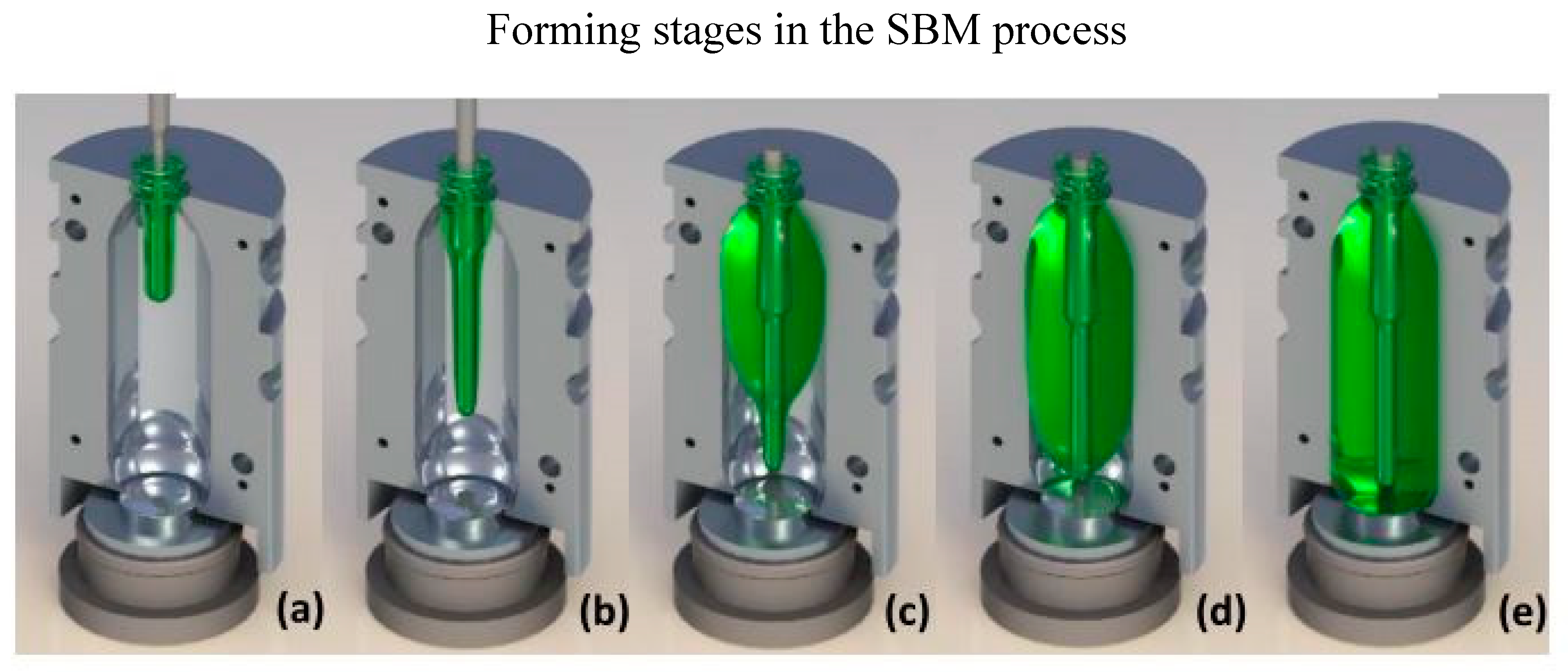
Figure 2.
Dimensions of preform used in experiments.
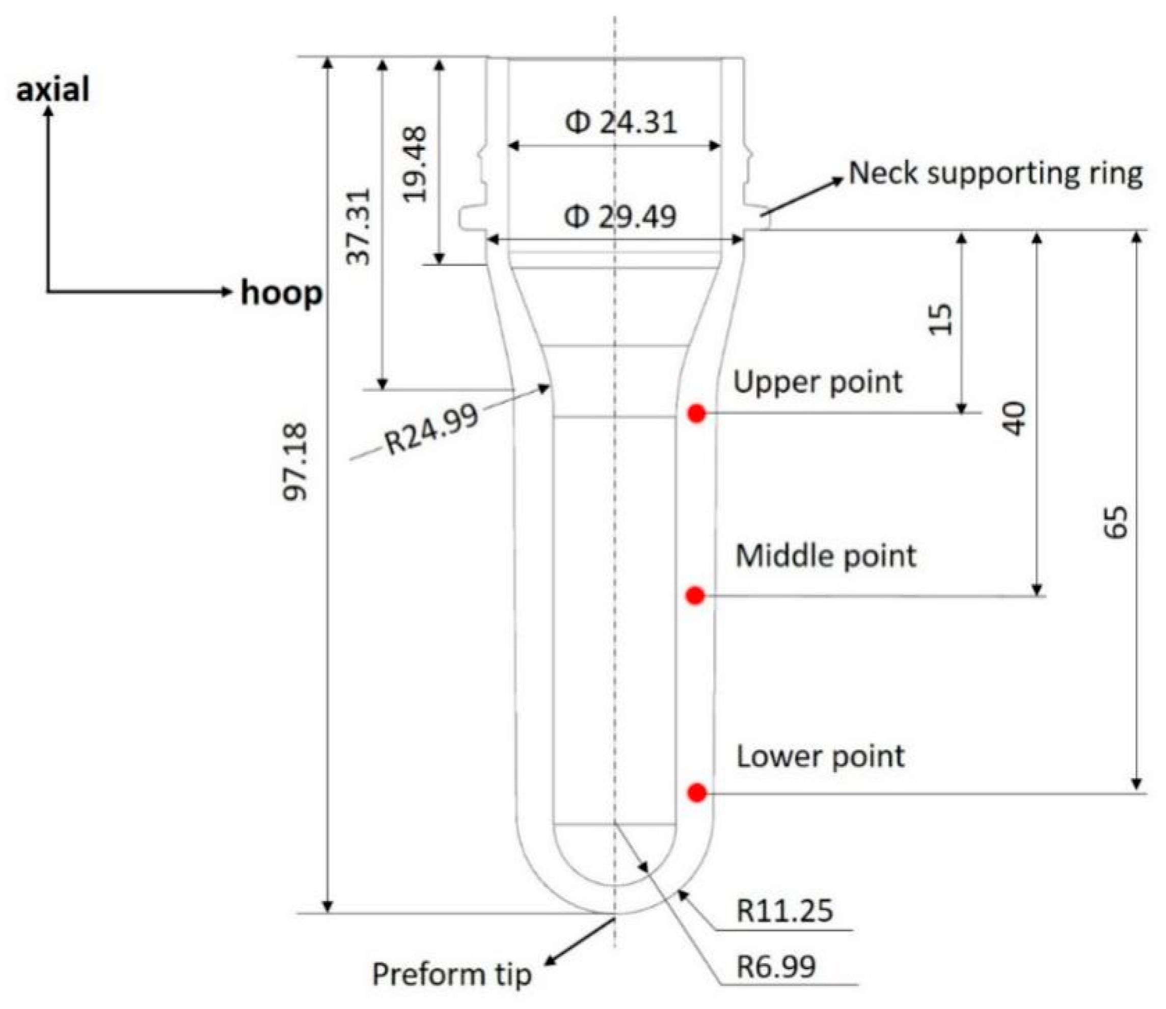
Figure 3.
Robotic controlled test rig, (a) the robotic arm used to hold the specimen;(b) oil bath device; (c) high speed cameras used for monitoring the deformation.
Figure 3.
Robotic controlled test rig, (a) the robotic arm used to hold the specimen;(b) oil bath device; (c) high speed cameras used for monitoring the deformation.
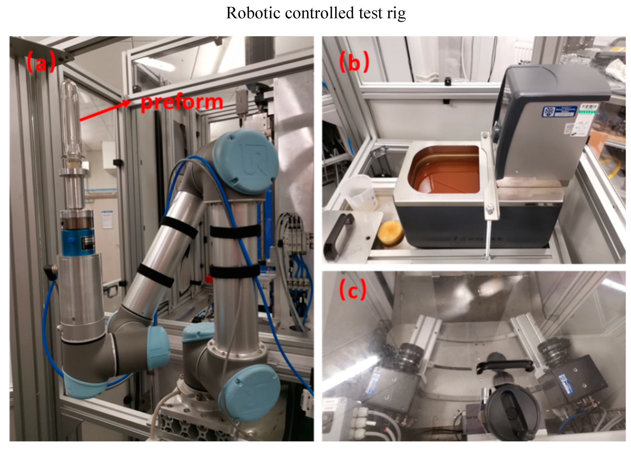
Figure 4.
Schematic diagram of demonstrating how stress strain data is captured from Free Stretch Blow experiments.
Figure 4.
Schematic diagram of demonstrating how stress strain data is captured from Free Stretch Blow experiments.
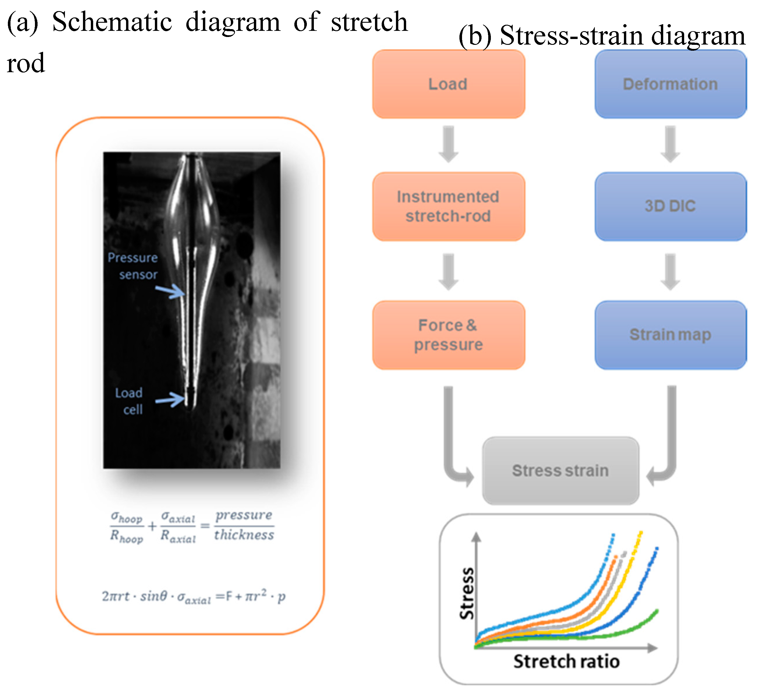
Figure 5.
Example of evolution of blowing preform monitored by high-speed camera with contours of hoop strain as calculated by Digital Image Correlation.
Figure 5.
Example of evolution of blowing preform monitored by high-speed camera with contours of hoop strain as calculated by Digital Image Correlation.
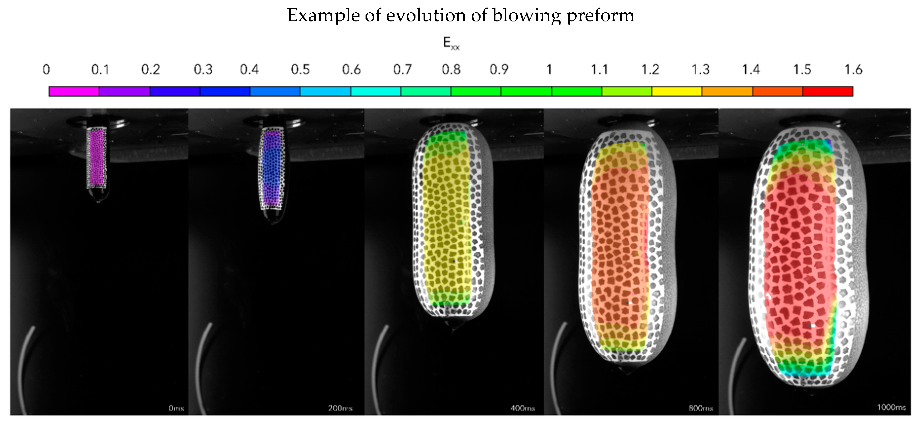
Figure 6.
The evolution of force and pressure of experiment shown in Figure 5.
Figure 6.
The evolution of force and pressure of experiment shown in Figure 5.
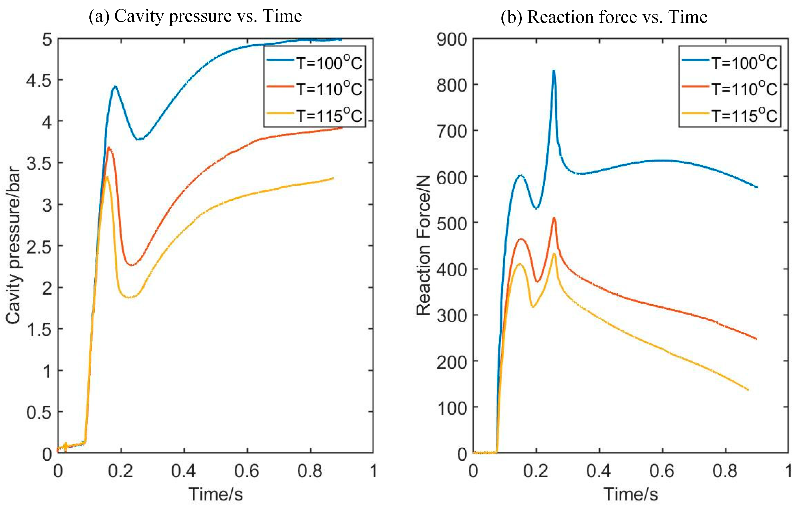
Figure 7.
An example of Hoop Stress Strain curves (a) and Axial Stress strain curves (b) from three positions of the preform (upper, middle, and lower as indicated in Figure 2).
Figure 7.
An example of Hoop Stress Strain curves (a) and Axial Stress strain curves (b) from three positions of the preform (upper, middle, and lower as indicated in Figure 2).
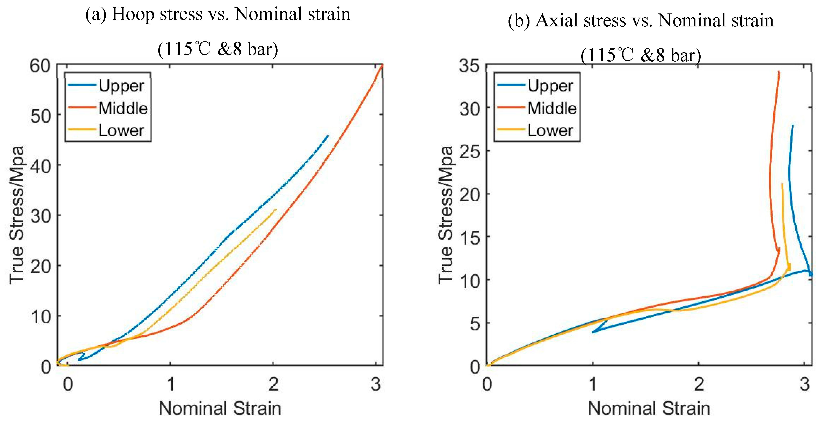
Figure 8.
An example of Hoop Stress Strain curves (a) and Axial Stress strain curves (b) from the midpoint of the preform for three different temperatures.
Figure 8.
An example of Hoop Stress Strain curves (a) and Axial Stress strain curves (b) from the midpoint of the preform for three different temperatures.
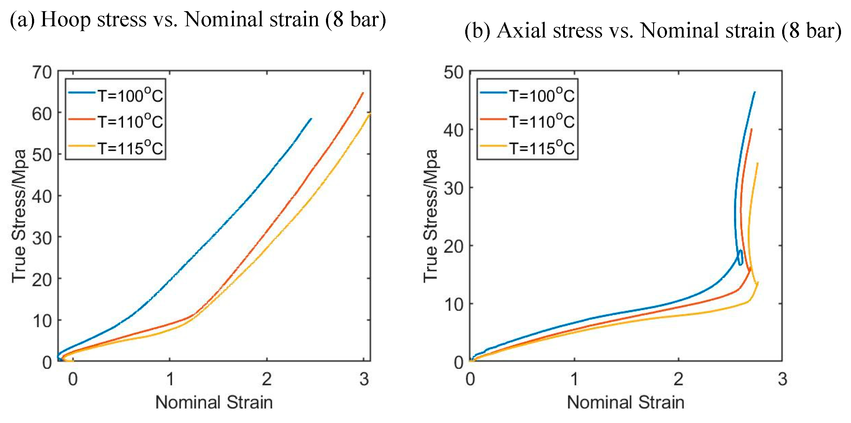
Figure 9.
A flow restrictor valve with a rotating knob.
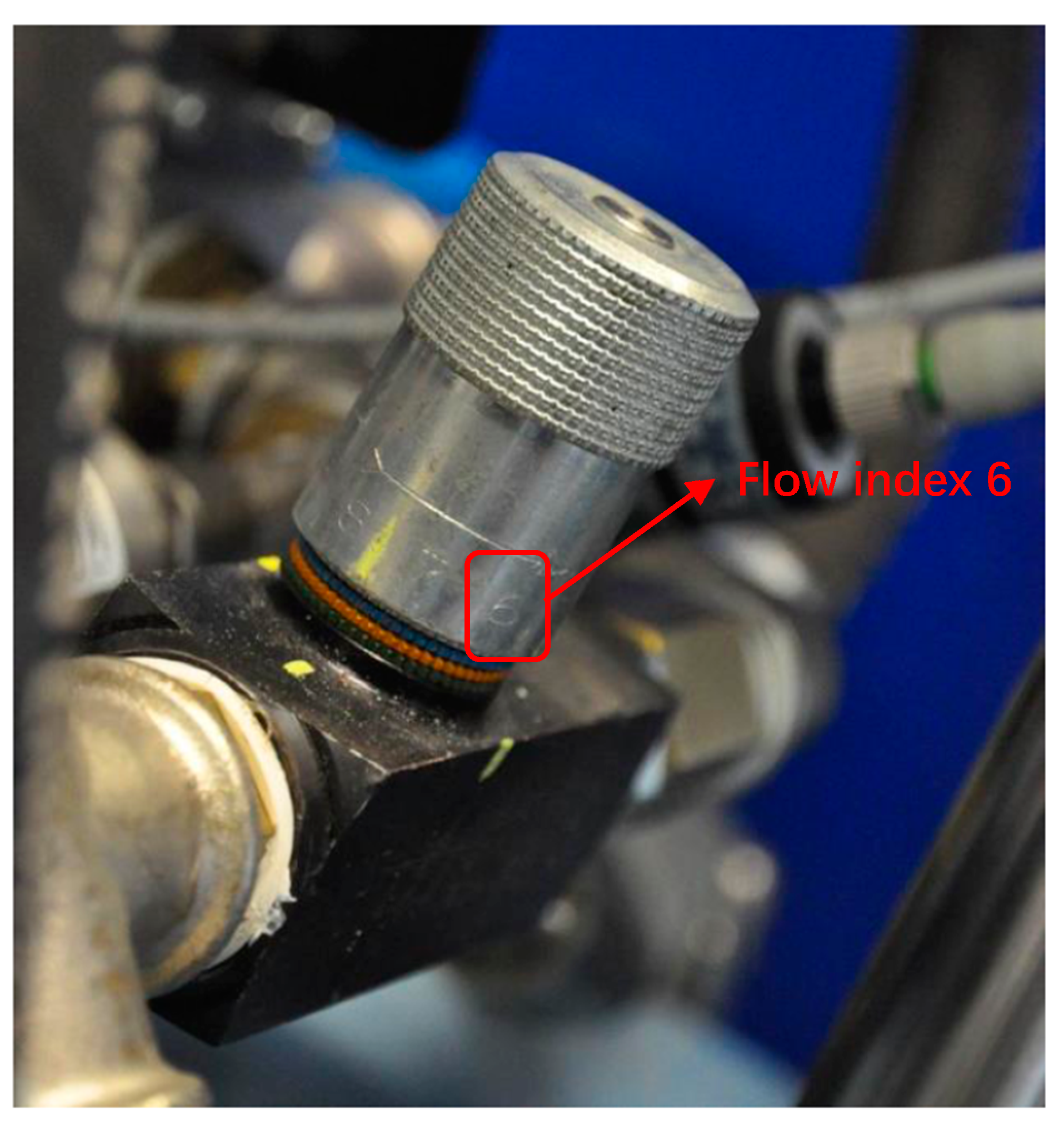
Figure 10.
Spring-dashpot illustration of the Buckley model.
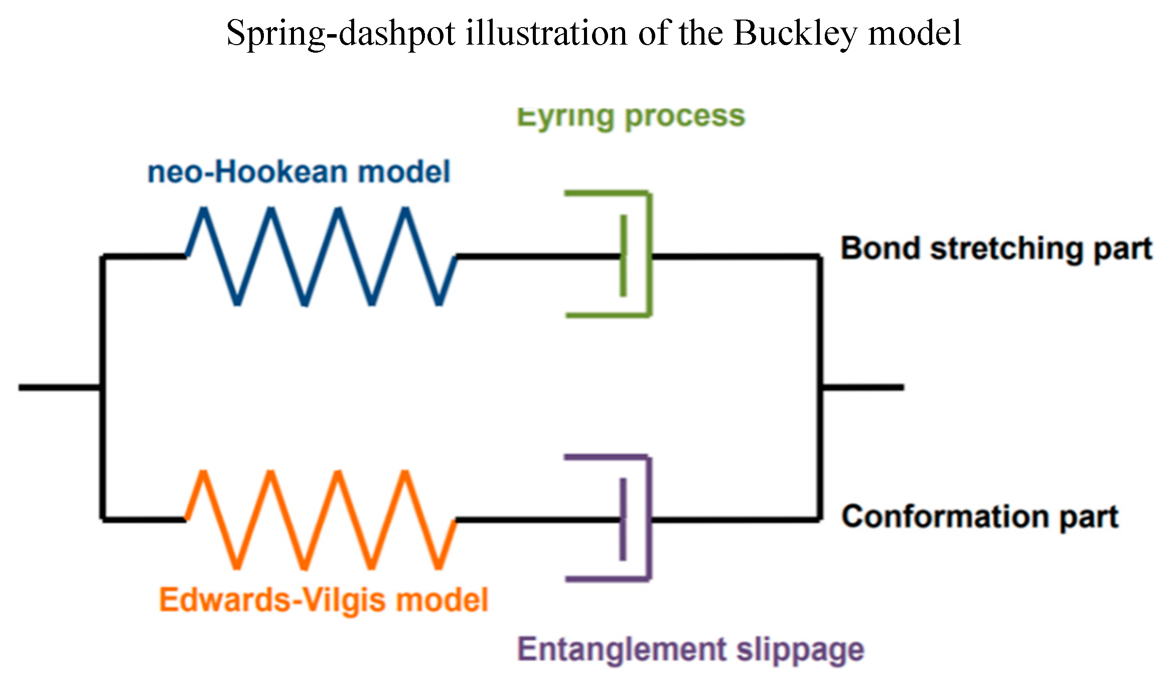
Figure 11.
Schematic diagram of hybrid ANN based model.
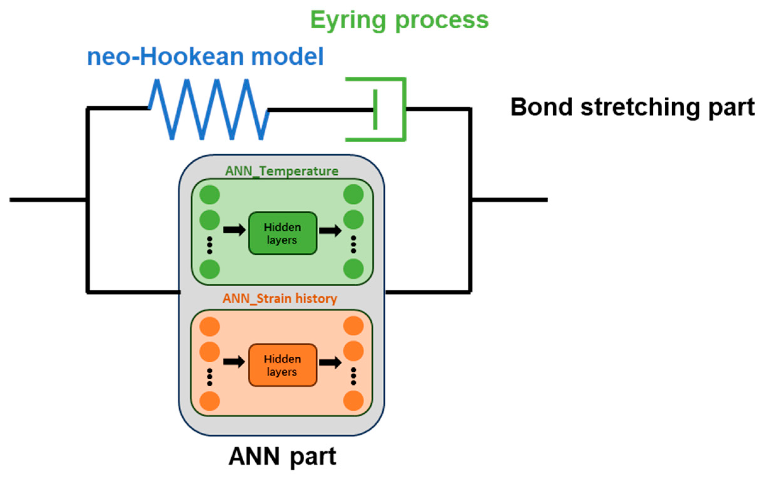
Figure 12.
An example of the relationship between Sb and Sc in both hoop (a) and axial (b) direction and partial enlargement views of (a) and (b). (The position of ‘Middle point’ is indicated in Figure 2).
Figure 12.
An example of the relationship between Sb and Sc in both hoop (a) and axial (b) direction and partial enlargement views of (a) and (b). (The position of ‘Middle point’ is indicated in Figure 2).
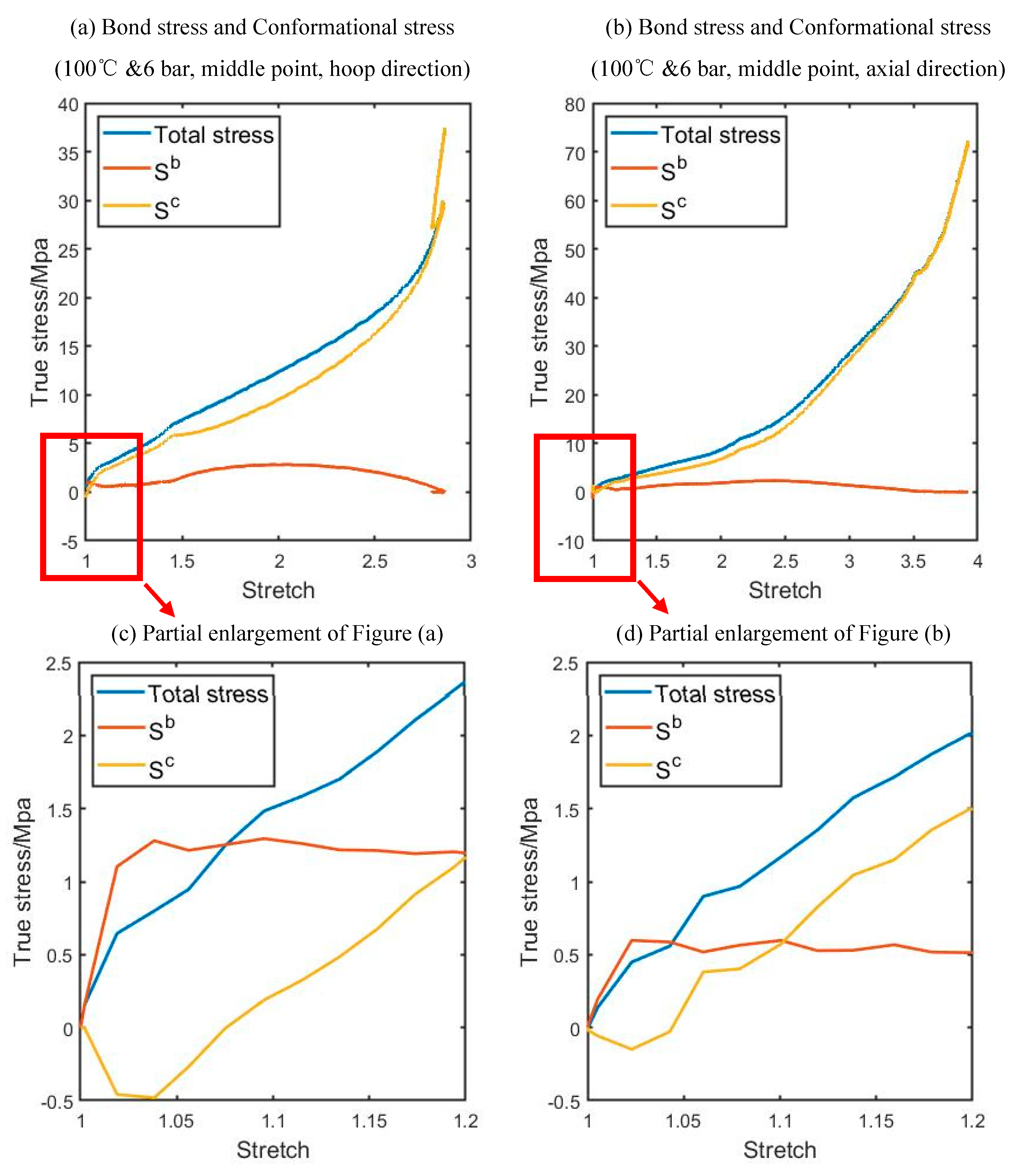
Figure 13.
the architecture of the ‘ANN_Temperature’.
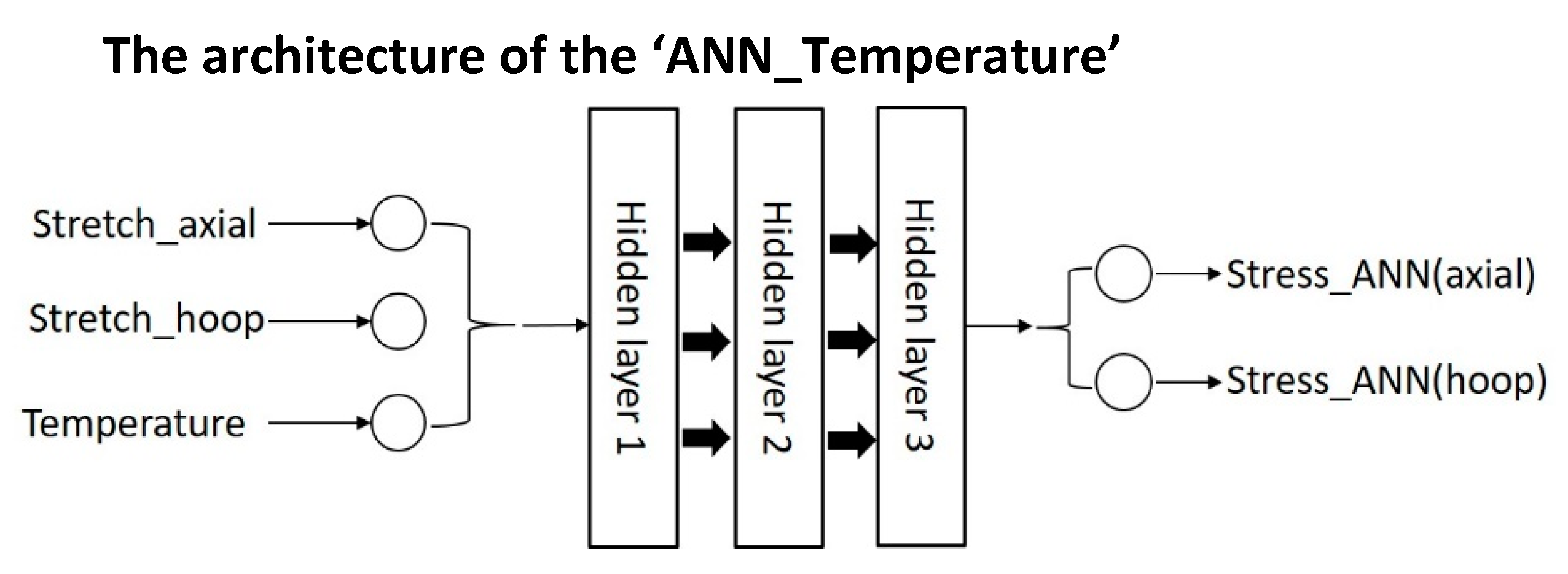
Figure 14.
The effect of mass flow rate and temperature on the maximum strain rate.
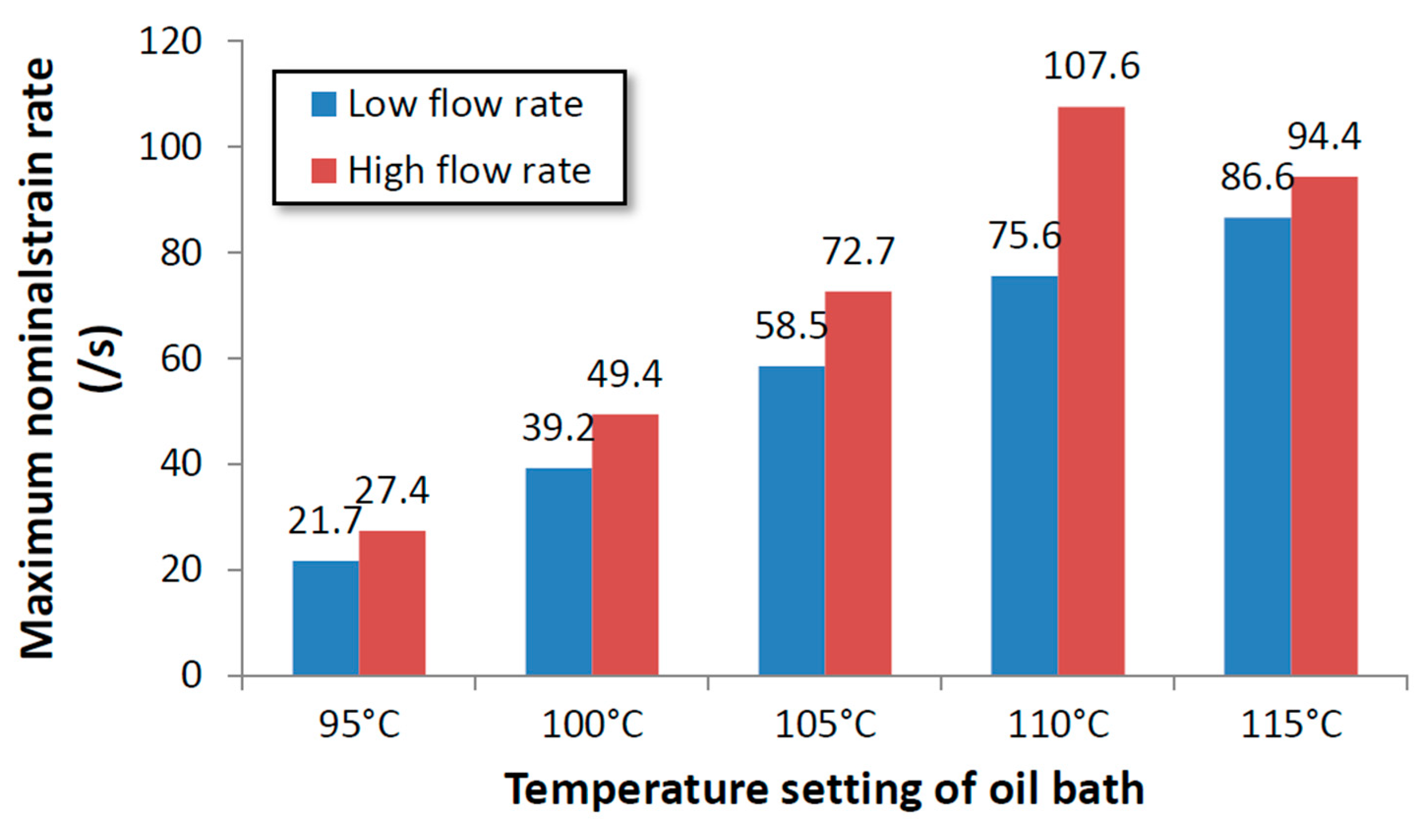
Figure 15.
The temperature increase produced by the high strain rate during SBM process.
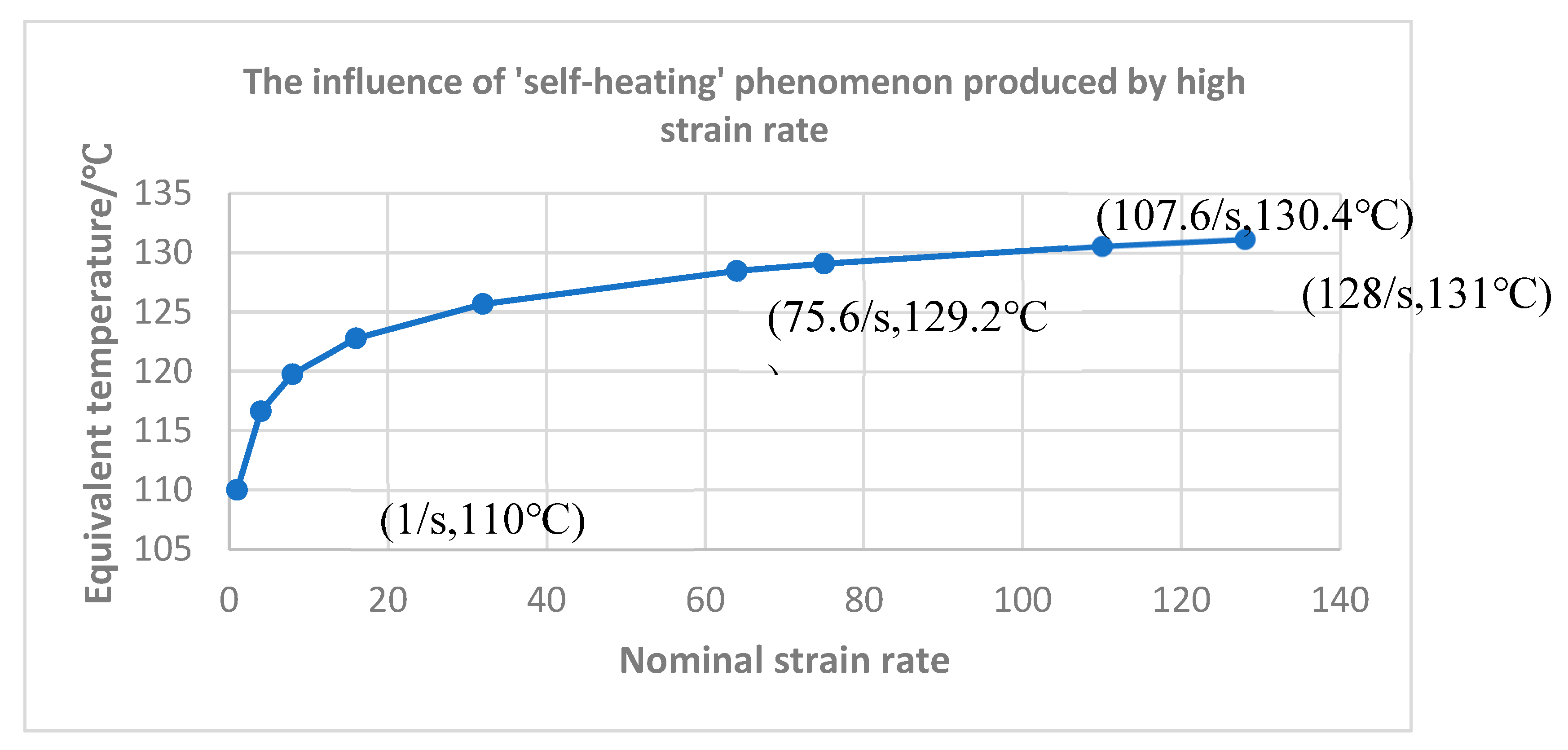
Figure 16.
equivalent stress-equivalent strain curves of selected points in P8N6T115.
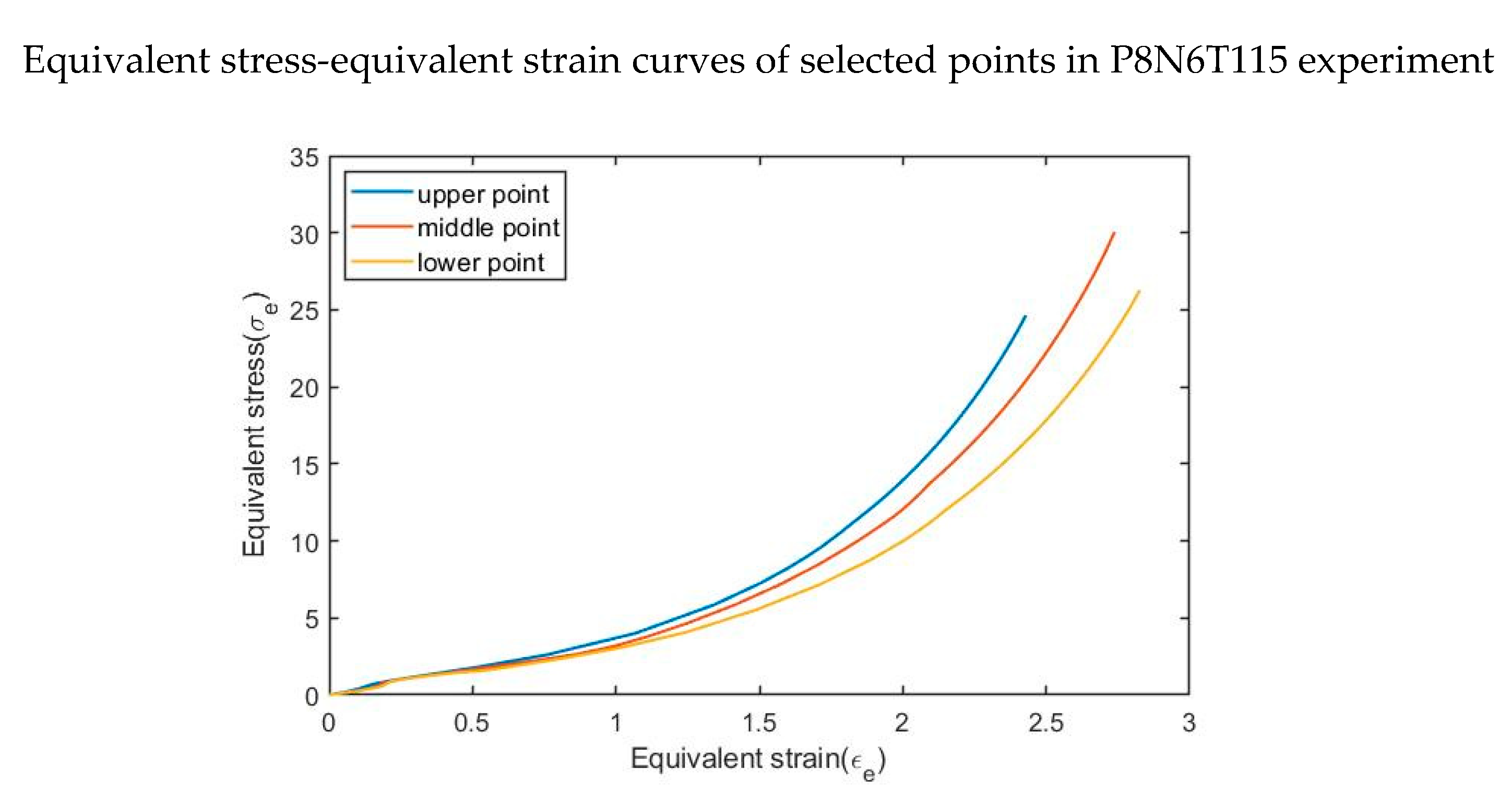
Figure 17.
The development of strain history of selected points in P8N2T115.
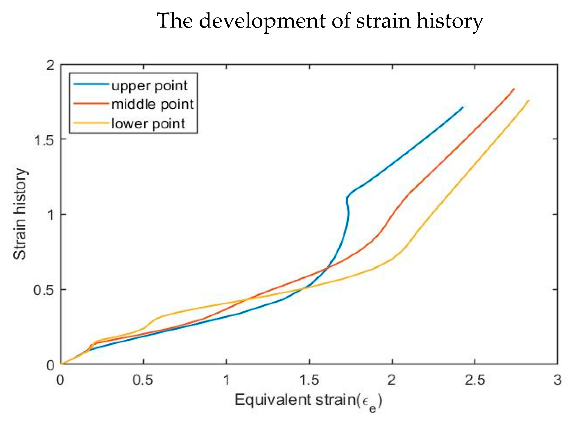
Figure 18.
the structure of the ‘ANN_Strain history’.
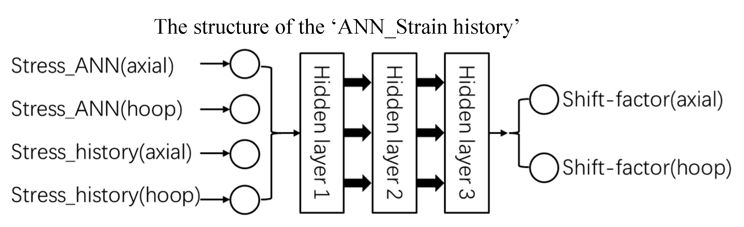
Figure 19.
Schematic diagram of ‘shift-factors’ for selected points in P8N6T115.
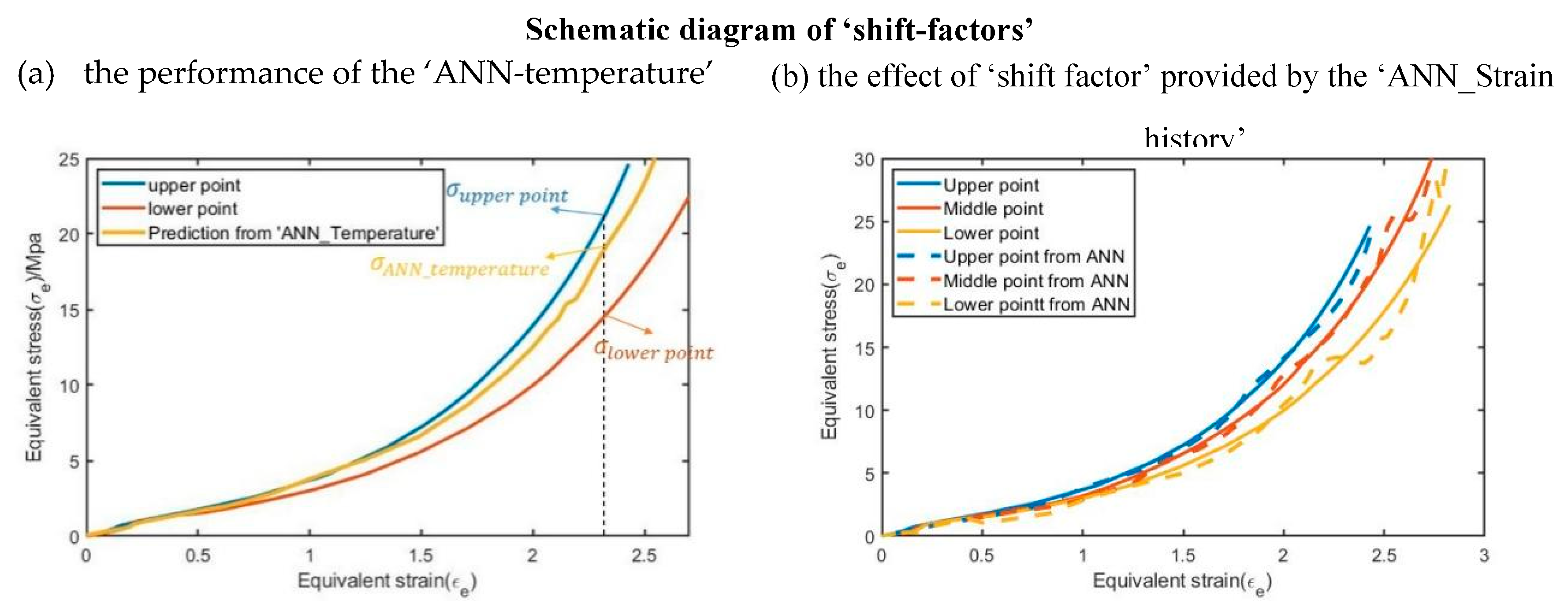
Figure 20.
Flow chart demonstrating the calculation procedure of the Hybrid ANN based constitutive model.
Figure 20.
Flow chart demonstrating the calculation procedure of the Hybrid ANN based constitutive model.
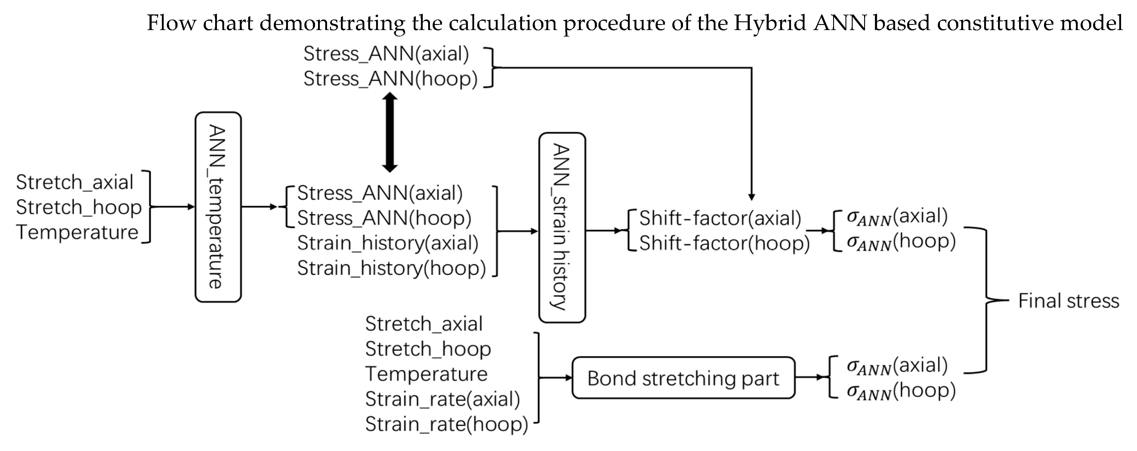
Figure 22.
detailed FE model used for free stretch blow simulation, (a) annotated CAE interface to illustrate the model of free stretch-blow process in ABAQUS/Explicit; (b) FE preform model with 80 SAX1 elements.
Figure 22.
detailed FE model used for free stretch blow simulation, (a) annotated CAE interface to illustrate the model of free stretch-blow process in ABAQUS/Explicit; (b) FE preform model with 80 SAX1 elements.
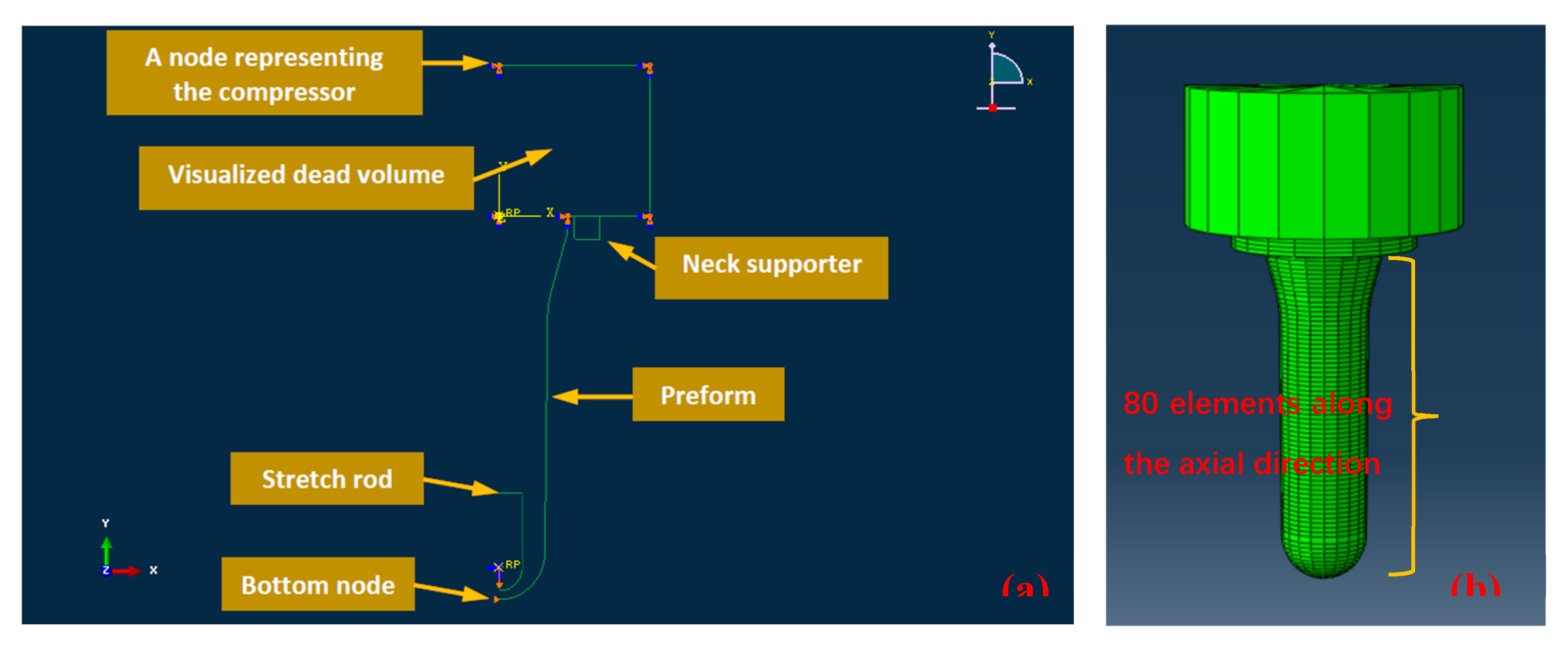
Figure 23.
illustration of distance between node pair, and the equation of calculating the average distance.
Figure 23.
illustration of distance between node pair, and the equation of calculating the average distance.
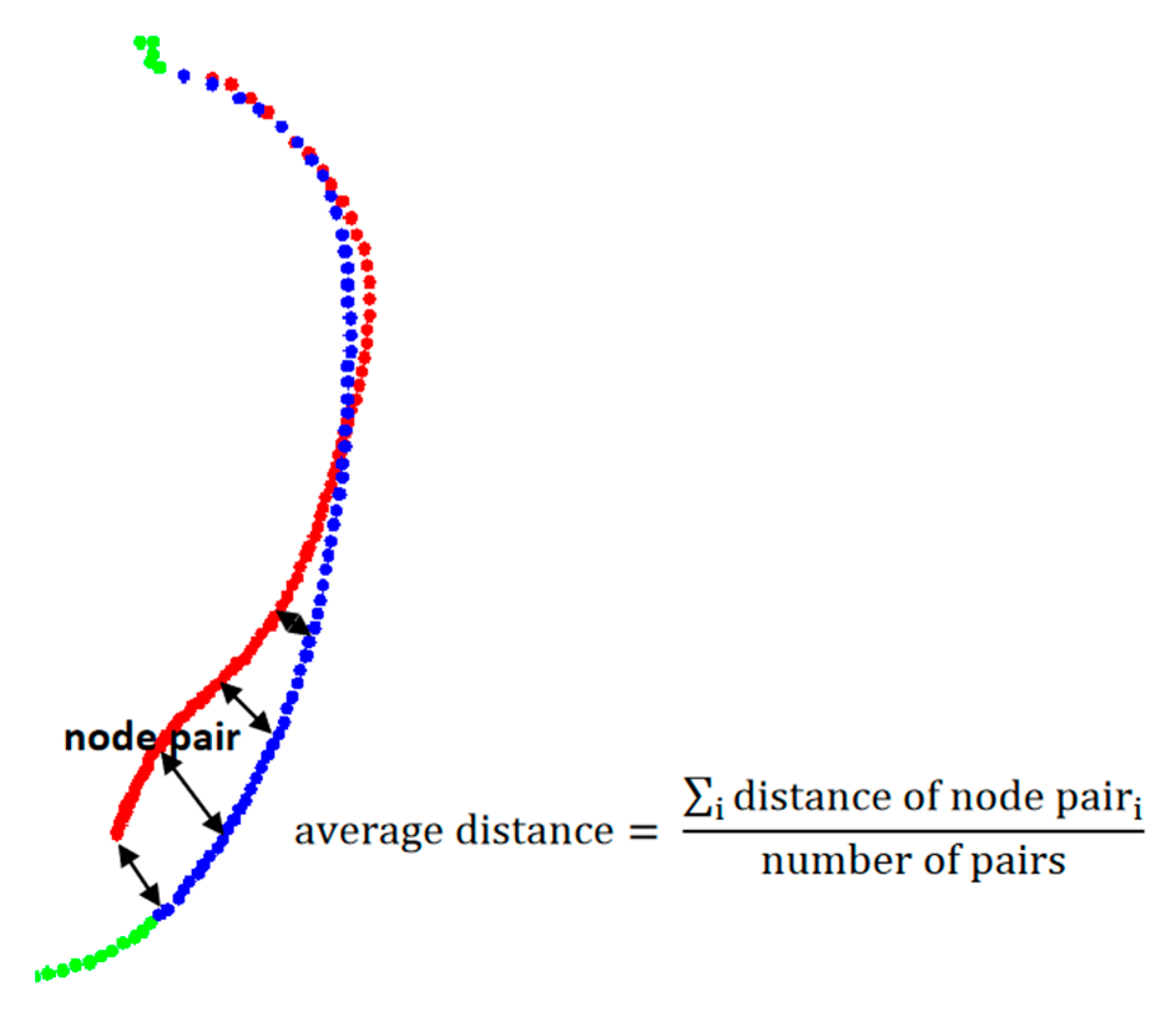
Figure 24.
Shape comparison of P8N2T110 in MATLAB.
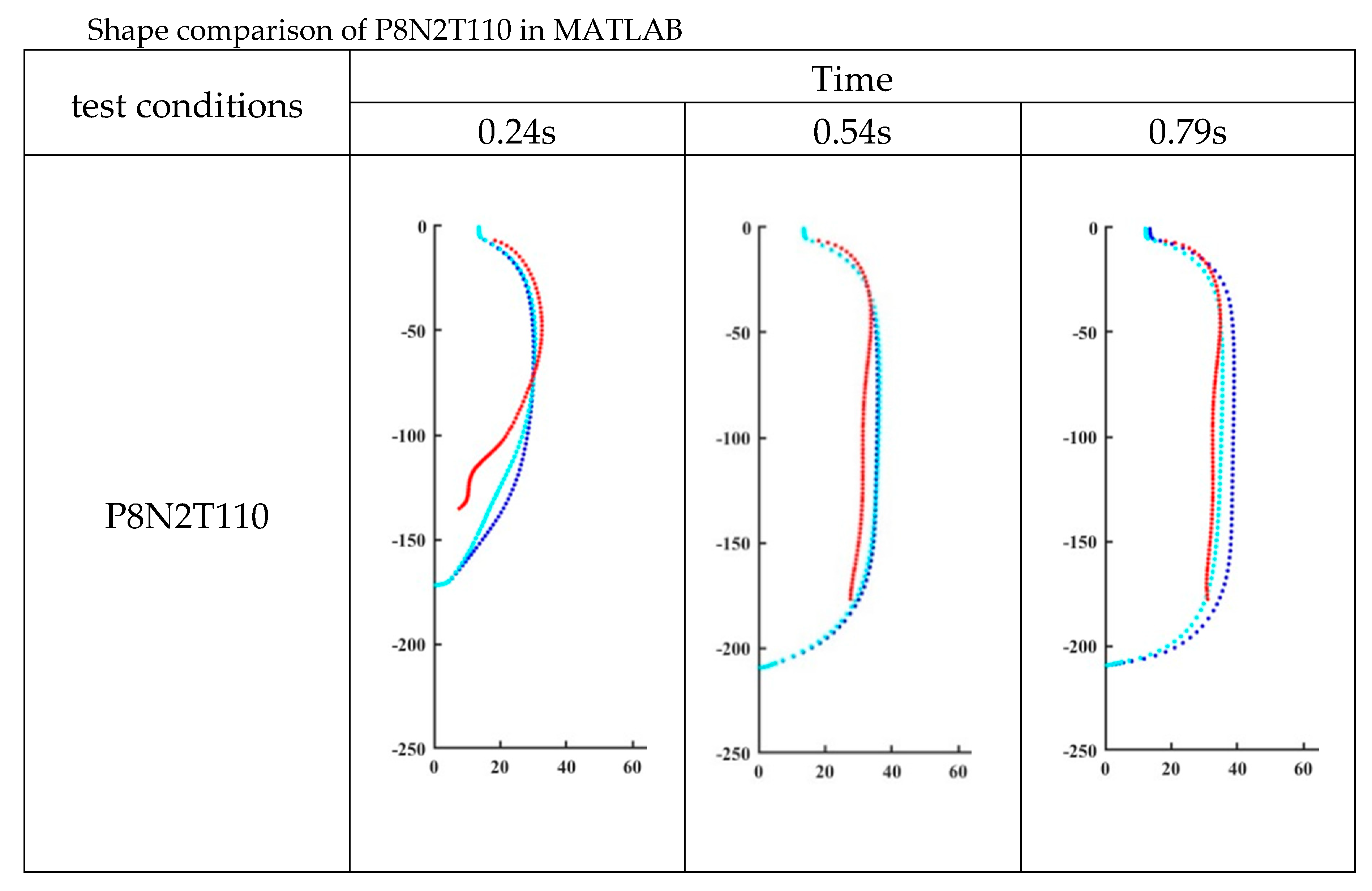
Figure 25.
Shape comparison of P8N2T115 in MATLAB.
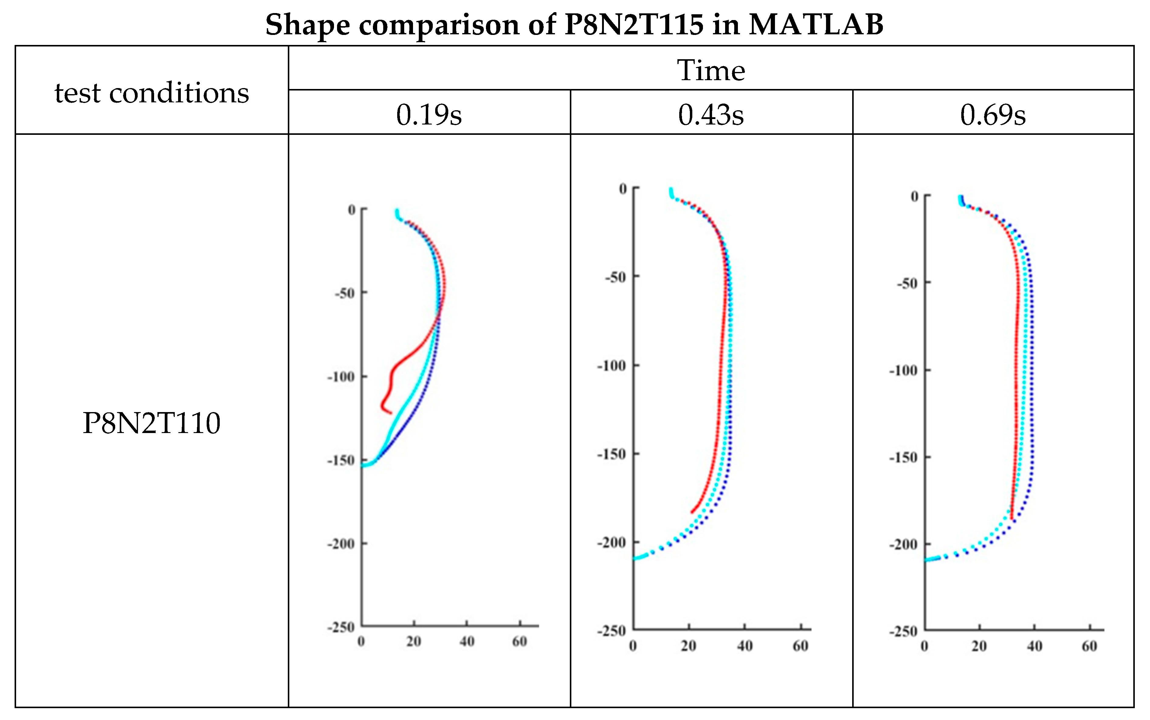
Table 1.
Summary of experiments conducted.
| Experiment label (Press/Flow/temp) |
Pressure, P (bar) | Flow index, N (1-6) | Temperature setting of oil bath( ℃ ) |
|---|---|---|---|
| P8N2T95 | 8 | 2 | 95 |
| P8N6T95 | 8 | 6 | 95 |
| P8N2T100 | 8 | 2 | 100 |
| P8N6T100 | 8 | 6 | 100 |
| P8N2T105 | 8 | 2 | 105 |
| P8N6T105 | 8 | 6 | 105 |
| P8N2T110 | 8 | 2 | 110 |
| P8N6T110 | 8 | 6 | 110 |
| P8N2T115 | 8 | 2 | 115 |
| P8N6T115 | 8 | 6 | 115 |
Table 2.
The Mean Relative Error(MRE) of experiments shown in Figure 20.
Table 2.
The Mean Relative Error(MRE) of experiments shown in Figure 20.
| Experiment label | Mean relative error |
|---|---|
| P8N2T95 | 1.37% |
| P8N6T95 | 1.16% |
| P8N2T100 | 2.14% |
| P8N6T100 | 2.42% |
| P8N2T105 | 2.57% |
| P8N6T110 | 2.00% |
| P8N6T115 | 4.14% |
Table 3.
Detailed ‘average distance’ of simulation results.
| Buckley model simulation | Hybrid ANN based constitutive mode simulation | |
|---|---|---|
| P8N2T110 | 8.11 | 6.21 |
| P8N2T115 | 12.39 | 8.83 |
Disclaimer/Publisher’s Note: The statements, opinions and data contained in all publications are solely those of the individual author(s) and contributor(s) and not of MDPI and/or the editor(s). MDPI and/or the editor(s) disclaim responsibility for any injury to people or property resulting from any ideas, methods, instructions or products referred to in the content. |
© 2024 by the authors. Licensee MDPI, Basel, Switzerland. This article is an open access article distributed under the terms and conditions of the Creative Commons Attribution (CC BY) license (http://creativecommons.org/licenses/by/4.0/).
Copyright: This open access article is published under a Creative Commons CC BY 4.0 license, which permit the free download, distribution, and reuse, provided that the author and preprint are cited in any reuse.


